Example 1 : As Simple as it Gets
Problem Statement
This example briefly describes the creation of a basic input file and the six required sections for utilizing MOOSE for solving a problem.
We consider the steady-state diffusion equation on the 3D domain : find such that , on the bottom, on the top and with on the remaining boundaries.
The weak form (see Finite Elements Principles) of this equation, in inner-product notation, is given by: , where are the test functions and is the finite element solution.
Input File Syntax
A basic moose input file requires six parts:
Mesh
Variables
Kernels
BCs
Executioner
Outputs
Mesh
The domain for the problem is created with the Mesh block in the input file. Here the mesh is read from the file mug.e which is a relative path starting in the same directory as the input file itself:
[Mesh]
  file = 'mug.e'
[]
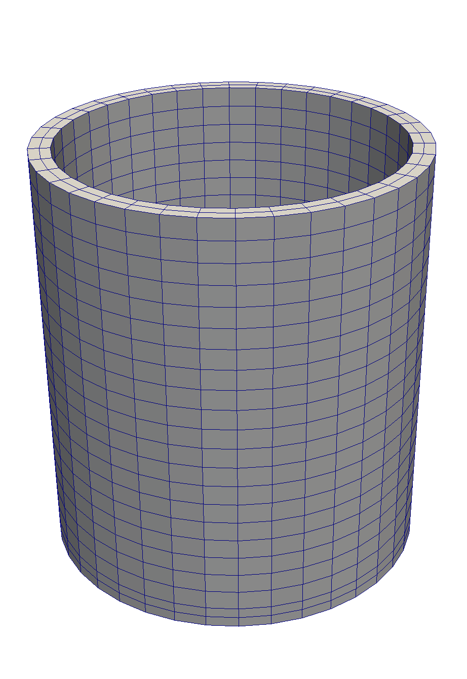
mug.e mesh file
Variables
In this simple problem, a single variable, 'diffused,' is defined, which represents from the continuous problem. The 'diffused' variable is approximated with linear Lagrange shape functions.
[Variables]
  [./diffused]
    order = FIRST
    family = LAGRANGE
  [../]
[]
Kernels
The weak form of the problem statement is represented by a Diffusion Kernel object. In general, users write custom Kernels that reside in their own MOOSE-based application(s), but in this case the Diffusion Kernel is already defined in MOOSE. To use a particular Kernel object an input file sub-section is defined, labeled "diff" (this is an arbitrary user-defined name), that utilizes the Diffusion Kernel and acts on the previously defined variable "diffused".
[Kernels]
  [./diff]
    type = Diffusion
    variable = diffused
  [../]
[]
Boundary Conditions (BCs)
Boundary conditions are defined in a manner similar to Kernels. For this problem two Dirichlet boundary conditions are required. In the input file the two boundary conditions are specified each using the DirichletBC object provided by MOOSE.
[BCs]
  [./bottom]
    # arbitrary user-chosen name
    type = DirichletBC
    variable = diffused
    boundary = 'bottom' # This must match a named boundary in the mesh file
    value = 1
  [../]

  [./top]
    # arbitrary user-chosen name
    type = DirichletBC
    variable = diffused
    boundary = 'top' # This must match a named boundary in the mesh file
    value = 0
  [../]
[]
Within each of the two sub-section, named "top" and "bottom" by the user, the boundary conditions are linked to their associated variable(s) (i.e. "diffused" in this case) and boundaries. In this case, the mesh file mug.e defines labeled the boundaries "top" and "bottom" which we can refer to. Boundaries will also often be specified by number IDs - depending on how your mesh file was generated.
Note, the Neumann boundary conditions for this problem (on the left and right sides) are satisfied implicitly and are not necessary for us to define. However, for non-zero Neumann or other boundary conditions many built-in objects are provided by MOOSE (e.g., NeumannBC). You can also create custom boundary conditions derived from the existing objects within MOOSE.
Executioner
The type of problem to solve and the method for solving it is defined within the Executioner block. This problem is steady-state and will use the Steady Executioner and will use the default solving method Preconditioned Jacobian Free Newton Krylov.
[Executioner]
  type = Steady
  solve_type = 'PJFNK'
[]
Outputs
Here two types of outputs are enabled: output to the screen (console) and output to an Exodus file (exodus). Setting the "file_base" parameter is optional, in this example it forces the output file to be named "out.e" ("e" is the extension used for the Exodus format).
[Outputs]
  execute_on = 'timestep_end'
  exodus = true
[]
Running the Problem
This example may be run using Peacock or by running the following commands form the command line.
cd ~/projects/moose/examples/ex01_inputfile
make -j8
./ex01-opt -i ex01.i
This will generate the results file, out.e, as shown in Figure 1. This file may be viewed using Peacock or an external application that supports the Exodus format (e.g., Paraview).
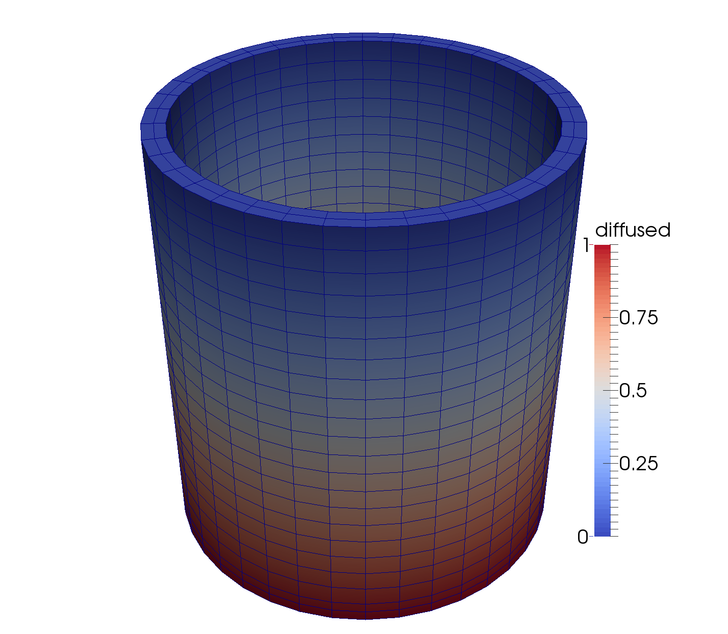
Figure 1: Example 1 Results
Next Steps
Although the Diffusion kernel is the only "physics" in the MOOSE framework, a large set of physics is included in the MOOSE modules. In order to implement your own physics, you will need to understand the following:
Finite Element Methods and the generating the "weak" form of for PDEs
C++ and object-oriented design
Check out more examples