Restarting and recovering from previous simulations
MOOSE provides several options for restarting or recovering from previous simulations. In this example, we demonstrate how this capability can be used in the PorousFlow module by considering a simple two-part problem. The first is to establish the hydrostatic pressure gradient in a reservoir that is due to gravity. This is the equilibrium state of the reservoir, and will be used as the initial condition for porepressure in the second part of this problem, where gas is injected into the reservoir in a single injection well.
Although this problem is simple, it demonstrates how the results of a previous simulation can be used to provide the initial condition for a second simulation.
Model
The properties of the reservoir used in the model are summarized in Table 1. The pressure gradient is representative of a reservoir at a depth of approximately 1,000 m.
Table 1: Reservoir properties
| Property | Value |
|---|---|
| Height | 100 m |
| Length | 5,000 m |
| Pressure | Hydrostatic (10 - 11 MPa) |
| Temperature | 50 C |
| Permeability | m (~100 md) |
| Porosity | 0.1 |
| NaCl mass fraction | 0.1 |
| Methane injection rate | 1 kg/s |
Relative permeability of the aqueous phase is represented by a Corey model, with exponent and residual saturation . Gas phase relative permeability is also represented using a Corey model, with exponent and residual saturation . Capillary pressure is given by a van Genuchten model, with exponent , and residual saturation .
Gravity equilibrium
The hydrostatic pressure gradient in the reservoir is the result of gravity and the density of the resident brine. This pressure gradient can be calculated using a fully saturated single-phase model with a relatively coarse mesh. As this pressure gradient depends on gravity, it develops in the vertical direction only, and can therefore be modelled using a two-dimensional Cartesian mesh.
The following input file to establish hydrostatic equilibrium in this model is provided:
# Initial run to establish gravity equilibrium. As only brine is present (no gas),
# we can use the single phase equation of state and kernels, reducing the computational
# cost. An estimate of the hydrostatic pressure gradient is used as the initial condition
# using an approximate brine density of 1060 kg/m^3.
# The end time is set to a large value (~100 years) to allow the pressure to reach
# equilibrium. Steady state detection is used to halt the run when a steady state is reached.

[Mesh<<<{"href": "../../syntax/Mesh/index.html"}>>>]
  type = GeneratedMesh
  dim = 2
  ny = 10
  nx = 10
  ymax = 100
  xmax = 5000
[]

[GlobalParams<<<{"href": "../../syntax/GlobalParams/index.html"}>>>]
  PorousFlowDictator = dictator
  gravity = '0 -9.81 0'
  temperature_unit = Celsius
[]

[Variables<<<{"href": "../../syntax/Variables/index.html"}>>>]
  [porepressure]
  []
[]

[ICs<<<{"href": "../../syntax/ICs/index.html"}>>>]
  [porepressure]
    type = FunctionIC<<<{"description": "An initial condition that uses a normal function of x, y, z to produce values (and optionally gradients) for a field variable.", "href": "../../source/ics/FunctionIC.html"}>>>
    function<<<{"description": "The initial condition function."}>>> = ppic
    variable<<<{"description": "The variable this initial condition is supposed to provide values for."}>>> = porepressure
  []
[]

[Functions<<<{"href": "../../syntax/Functions/index.html"}>>>]
  [ppic]
    type = ParsedFunction<<<{"description": "Function created by parsing a string", "href": "../../source/functions/MooseParsedFunction.html"}>>>
    expression<<<{"description": "The user defined function."}>>> = '10e6 + 1060*9.81*(100-y)'
  []
[]

[BCs<<<{"href": "../../syntax/BCs/index.html"}>>>]
  [top]
    type = DirichletBC<<<{"description": "Imposes the essential boundary condition $u=g$, where $g$ is a constant, controllable value.", "href": "../../source/bcs/DirichletBC.html"}>>>
    variable<<<{"description": "The name of the variable that this residual object operates on"}>>> = porepressure
    value<<<{"description": "Value of the BC"}>>> = 10e6
    boundary<<<{"description": "The list of boundary IDs from the mesh where this object applies"}>>> = top
  []
[]

[AuxVariables<<<{"href": "../../syntax/AuxVariables/index.html"}>>>]
  [temperature]
    initial_condition<<<{"description": "Specifies a constant initial condition for this variable"}>>> = 50
  []
  [xnacl]
    initial_condition<<<{"description": "Specifies a constant initial condition for this variable"}>>> = 0.1
  []
  [brine_density]
    family<<<{"description": "Specifies the family of FE shape functions to use for this variable"}>>> = MONOMIAL
    order<<<{"description": "Specifies the order of the FE shape function to use for this variable (additional orders not listed are allowed)"}>>> = CONSTANT
  []
[]

[Kernels<<<{"href": "../../syntax/Kernels/index.html"}>>>]
  [mass0]
    type = PorousFlowMassTimeDerivative<<<{"description": "Derivative of fluid-component mass with respect to time.  Mass lumping to the nodes is used.", "href": "../../source/kernels/PorousFlowMassTimeDerivative.html"}>>>
    variable<<<{"description": "The name of the variable that this residual object operates on"}>>> = porepressure
  []
  [flux0]
    type = PorousFlowFullySaturatedDarcyFlow<<<{"description": "Darcy flux suitable for models involving a fully-saturated single phase, multi-component fluid.  No upwinding is used", "href": "../../source/kernels/PorousFlowFullySaturatedDarcyFlow.html"}>>>
    variable<<<{"description": "The name of the variable that this residual object operates on"}>>> = porepressure
  []
[]

[AuxKernels<<<{"href": "../../syntax/AuxKernels/index.html"}>>>]
  [brine_density]
    type = PorousFlowPropertyAux<<<{"description": "AuxKernel to provide access to properties evaluated at quadpoints. Note that elemental AuxVariables must be used, so that these properties are integrated over each element.", "href": "../../source/auxkernels/PorousFlowPropertyAux.html"}>>>
    property<<<{"description": "The fluid property that this auxillary kernel is to calculate"}>>> = density
    variable<<<{"description": "The name of the variable that this object applies to"}>>> = brine_density
    execute_on<<<{"description": "The list of flag(s) indicating when this object should be executed. For a description of each flag, see https://mooseframework.inl.gov/source/interfaces/SetupInterface.html."}>>> = 'initial timestep_end'
  []
[]

[UserObjects<<<{"href": "../../syntax/UserObjects/index.html"}>>>]
  [dictator]
    type = PorousFlowDictator<<<{"description": "Holds information on the PorousFlow variable names", "href": "../../source/userobjects/PorousFlowDictator.html"}>>>
    porous_flow_vars<<<{"description": "List of primary variables that are used in the PorousFlow simulation.  Jacobian entries involving derivatives wrt these variables will be computed.  In single-phase models you will just have one (eg 'pressure'), in two-phase models you will have two (eg 'p_water p_gas', or 'p_water s_water'), etc."}>>> = porepressure
    number_fluid_phases<<<{"description": "The number of fluid phases in the simulation"}>>> = 1
    number_fluid_components<<<{"description": "The number of fluid components in the simulation"}>>> = 1
  []
[]

[FluidProperties<<<{"href": "../../syntax/FluidProperties/index.html"}>>>]
  [brine]
    type = BrineFluidProperties<<<{"description": "Fluid properties for brine", "href": "../../source/fluidproperties/BrineFluidProperties.html"}>>>
  []
[]

[Materials<<<{"href": "../../syntax/Materials/index.html"}>>>]
  [temperature]
    type = PorousFlowTemperature<<<{"description": "Material to provide temperature at the quadpoints or nodes and derivatives of it with respect to the PorousFlow variables", "href": "../../source/materials/PorousFlowTemperature.html"}>>>
    temperature<<<{"description": "Fluid temperature variable.  Note, the default is suitable if your simulation is using Kelvin units, but probably not for Celsius"}>>> = temperature
  []
  [ps]
    type = PorousFlow1PhaseFullySaturated<<<{"description": "This Material is used for the fully saturated single-phase situation where porepressure is the primary variable", "href": "../../source/materials/PorousFlow1PhaseFullySaturated.html"}>>>
    porepressure<<<{"description": "Variable that represents the porepressure of the single phase"}>>> = porepressure
  []
  [massfrac]
    type = PorousFlowMassFraction<<<{"description": "This Material forms a std::vector<std::vector ...> of mass-fractions out of the individual mass fractions", "href": "../../source/materials/PorousFlowMassFraction.html"}>>>
  []
  [brine]
    type = PorousFlowBrine<<<{"description": "This Material calculates fluid properties for brine at the quadpoints or nodes", "href": "../../source/materials/PorousFlowBrine.html"}>>>
    compute_enthalpy<<<{"description": "Compute the fluid enthalpy"}>>> = false
    compute_internal_energy<<<{"description": "Compute the fluid internal energy"}>>> = false
    xnacl<<<{"description": "The salt mass fraction in the brine (kg/kg)"}>>> = xnacl
    phase<<<{"description": "The phase number"}>>> = 0
  []
  [porosity]
    type = PorousFlowPorosityConst<<<{"description": "This Material calculates the porosity assuming it is constant", "href": "../../source/materials/PorousFlowPorosityConst.html"}>>>
    porosity<<<{"description": "The porosity (assumed indepenent of porepressure, temperature, strain, etc, for this material).  This should be a real number, or a constant monomial variable (not a linear lagrange or other kind of variable)."}>>> = 0.1
  []
  [permeability]
    type = PorousFlowPermeabilityConst<<<{"description": "This Material calculates the permeability tensor assuming it is constant", "href": "../../source/materials/PorousFlowPermeabilityConst.html"}>>>
    permeability<<<{"description": "The permeability tensor (usually in m^2), which is assumed constant for this material"}>>> = '1e-13 0 0 0 1e-13 0  0 0 1e-13'
  []
[]

[Preconditioning<<<{"href": "../../syntax/Preconditioning/index.html"}>>>]
  [smp]
    type = SMP<<<{"description": "Single matrix preconditioner (SMP) builds a preconditioner using user defined off-diagonal parts of the Jacobian.", "href": "../../source/preconditioners/SingleMatrixPreconditioner.html"}>>>
    full<<<{"description": "Set to true if you want the full set of couplings between variables simply for convenience so you don't have to set every off_diag_row and off_diag_column combination."}>>> = true
  []
[]

[Executioner<<<{"href": "../../syntax/Executioner/index.html"}>>>]
  type = Transient
  solve_type = Newton
  end_time = 3e9
  nl_abs_tol = 1e-12
  nl_rel_tol = 1e-06
  steady_state_detection = true
  steady_state_tolerance = 1e-12
  [TimeStepper<<<{"href": "../../syntax/Executioner/TimeStepper/index.html"}>>>]
    type = IterationAdaptiveDT
    dt = 1e1
  []
[]

[Outputs<<<{"href": "../../syntax/Outputs/index.html"}>>>]
  execute_on<<<{"description": "The list of flag(s) indicating when this object should be executed. For a description of each flag, see https://mooseframework.inl.gov/source/interfaces/SetupInterface.html."}>>> = 'initial timestep_end'
  exodus<<<{"description": "Output the results using the default settings for Exodus output."}>>> = true
  perf_graph<<<{"description": "Enable printing of the performance graph to the screen (Console)"}>>> = true
[]In this example, an initial guess at the hydrostatic equilibrium is provided using a function with an estimate of the brine density at the given pressure and temperature (approximately 1060 kg/m)
[Functions<<<{"href": "../../syntax/Functions/index.html"}>>>]
  [ppic]
    type = ParsedFunction<<<{"description": "Function created by parsing a string", "href": "../../source/functions/MooseParsedFunction.html"}>>>
    expression<<<{"description": "The user defined function."}>>> = '10e6 + 1060*9.81*(100-y)'
  []
[]The simulation is set to run for approximately 100 years, with steady-state detection enabled to end the run when a steady-state solution has been found
[Executioner<<<{"href": "../../syntax/Executioner/index.html"}>>>]
  type = Transient
  solve_type = Newton
  end_time = 3e9
  nl_abs_tol = 1e-12
  nl_rel_tol = 1e-06
  steady_state_detection = true
  steady_state_tolerance = 1e-12
  [TimeStepper<<<{"href": "../../syntax/Executioner/TimeStepper/index.html"}>>>]
    type = IterationAdaptiveDT
    dt = 1e1
  []
[]This input file quickly establishes gravity equilibrium in twelve time steps, with a hydrostatic pressure gradient shown in Figure 1.
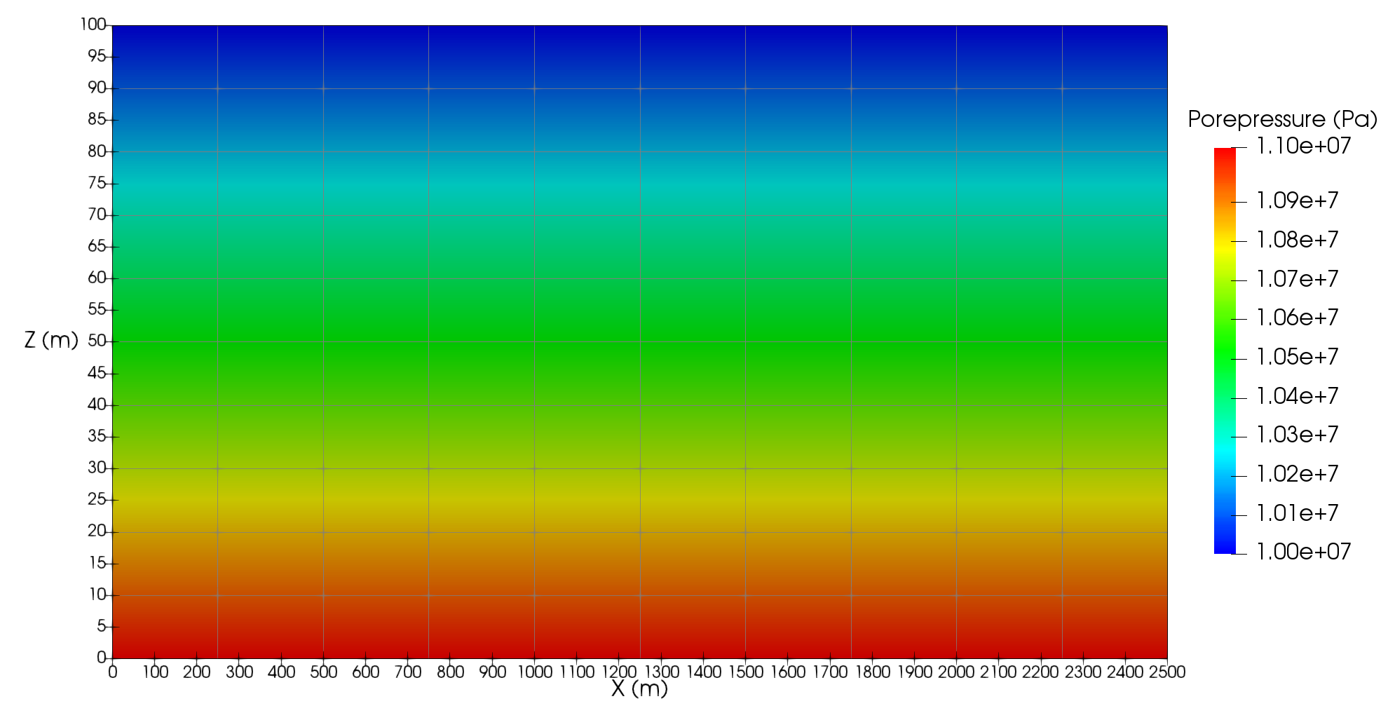
Figure 1: Hydrostatic pressure gradient at gravity equilibrium
Basic restart
The results of the gravity equilibrium simulation can be used as initial conditions for a more complicated simulation. In this case, we now consider injection of methane through an injection well in a two-dimensional radial model constructed by rotating the mesh used in the gravity equilibrium run around the Y-axis.
In contrast to the simple gravity equilibrium model, we now use a two-phase model, with the initial condition for the liquid porepressure taken from the final results of the gravity equilibrium simulation.
As the mesh is identical in both cases (despite the rotation about the Y-axis), we can use the simple variable initialisation available in MOOSE.
The input file for this case is
# Using the results from the equilibrium run to provide the initial condition for
# porepressure, we now inject a gas phase into the brine-saturated reservoir. In this
# example, where the mesh used is identical to the mesh used in gravityeq.i, we can use
# the basic restart capability by simply setting the initial condition for porepressure
# using the results from gravityeq.i.
#
# Even though the gravity equilibrium is established using a 2D mesh, in this example,
# we shift the mesh 0.1 m to the right and rotate it about the Y axis to make a 2D radial
# model.
#
# Methane injection takes place over the surface of the hole created by rotating the mesh,
# and hence the injection area is 2 pi r h. We can calculate this using an AreaPostprocessor,
# and then use this in a ParsedFunction to calculate the injection rate so that 10 kg/s of
# methane is injected.
#
# Results can be improved by uniformly refining the initial mesh.
#
# Note: as this example uses the results from a previous simulation, gravityeq.i MUST be
# run before running this input file.

[Mesh<<<{"href": "../../syntax/Mesh/index.html"}>>>]
  uniform_refine<<<{"description": "Specify the level of uniform refinement applied to the initial mesh"}>>> = 1
  [file]
    type = FileMeshGenerator<<<{"description": "Read a mesh from a file.", "href": "../../source/meshgenerators/FileMeshGenerator.html"}>>>
    file<<<{"description": "The filename to read."}>>> = gravityeq_out.e
  []
  [translate]
    type = TransformGenerator<<<{"description": "Applies a linear transform to the entire mesh.", "href": "../../source/meshgenerators/TransformGenerator.html"}>>>
    transform<<<{"description": "The type of transformation to perform (TRANSLATE, TRANSLATE_CENTER_ORIGIN, TRANSLATE_MIN_ORIGIN, ROTATE, SCALE, ROTATE_WITH_MATRIX, ROTATE_EXT)"}>>> = TRANSLATE
    vector_value<<<{"description": "The value to use for the transformation. When using TRANSLATE or SCALE, the xyz coordinates are applied in each direction respectively. When using ROTATE, the values are interpreted as the Euler angles phi, theta and psi given in degrees. For ROTATE_EXT, an extrinsic rotation is carried out using prescribed Euler angles alpha, beta, and gamma in degrees."}>>> = '0.1 0 0'
    input<<<{"description": "The mesh we want to modify"}>>> = file
  []
  coord_type = RZ
  rz_coord_axis = Y
[]

[GlobalParams<<<{"href": "../../syntax/GlobalParams/index.html"}>>>]
  PorousFlowDictator = dictator
  gravity = '0 -9.81 0'
  temperature_unit = Celsius
[]

[Variables<<<{"href": "../../syntax/Variables/index.html"}>>>]
  [pp_liq]
    initial_from_file_var<<<{"description": "Gives the name of a variable for which to read an initial condition from a mesh file"}>>> = porepressure
  []
  [sat_gas]
    initial_condition<<<{"description": "Specifies a constant initial condition for this variable"}>>> = 0
  []
[]

[AuxVariables<<<{"href": "../../syntax/AuxVariables/index.html"}>>>]
  [temperature]
    initial_condition<<<{"description": "Specifies a constant initial condition for this variable"}>>> = 50
  []
  [xnacl]
    initial_condition<<<{"description": "Specifies a constant initial condition for this variable"}>>> = 0.1
  []
  [brine_density]
    family<<<{"description": "Specifies the family of FE shape functions to use for this variable"}>>> = MONOMIAL
    order<<<{"description": "Specifies the order of the FE shape function to use for this variable (additional orders not listed are allowed)"}>>> = CONSTANT
  []
  [methane_density]
    family<<<{"description": "Specifies the family of FE shape functions to use for this variable"}>>> = MONOMIAL
    order<<<{"description": "Specifies the order of the FE shape function to use for this variable (additional orders not listed are allowed)"}>>> = CONSTANT
  []
  [massfrac_ph0_sp0]
    initial_condition<<<{"description": "Specifies a constant initial condition for this variable"}>>> = 1
  []
  [massfrac_ph1_sp0]
    initial_condition<<<{"description": "Specifies a constant initial condition for this variable"}>>> = 0
  []
  [pp_gas]
    family<<<{"description": "Specifies the family of FE shape functions to use for this variable"}>>> = MONOMIAL
    order<<<{"description": "Specifies the order of the FE shape function to use for this variable (additional orders not listed are allowed)"}>>> = CONSTANT
  []
  [sat_liq]
    family<<<{"description": "Specifies the family of FE shape functions to use for this variable"}>>> = MONOMIAL
    order<<<{"description": "Specifies the order of the FE shape function to use for this variable (additional orders not listed are allowed)"}>>> = CONSTANT
  []
[]

[Kernels<<<{"href": "../../syntax/Kernels/index.html"}>>>]
  [mass0]
    type = PorousFlowMassTimeDerivative<<<{"description": "Derivative of fluid-component mass with respect to time.  Mass lumping to the nodes is used.", "href": "../../source/kernels/PorousFlowMassTimeDerivative.html"}>>>
    variable<<<{"description": "The name of the variable that this residual object operates on"}>>> = pp_liq
  []
  [flux0]
    type = PorousFlowAdvectiveFlux<<<{"description": "Fully-upwinded advective flux of the component given by fluid_component", "href": "../../source/kernels/PorousFlowAdvectiveFlux.html"}>>>
    variable<<<{"description": "The name of the variable that this residual object operates on"}>>> = pp_liq
  []
  [mass1]
    type = PorousFlowMassTimeDerivative<<<{"description": "Derivative of fluid-component mass with respect to time.  Mass lumping to the nodes is used.", "href": "../../source/kernels/PorousFlowMassTimeDerivative.html"}>>>
    variable<<<{"description": "The name of the variable that this residual object operates on"}>>> = sat_gas
    fluid_component<<<{"description": "The index corresponding to the component for this kernel"}>>> = 1
  []
  [flux1]
    type = PorousFlowAdvectiveFlux<<<{"description": "Fully-upwinded advective flux of the component given by fluid_component", "href": "../../source/kernels/PorousFlowAdvectiveFlux.html"}>>>
    variable<<<{"description": "The name of the variable that this residual object operates on"}>>> = sat_gas
    fluid_component<<<{"description": "The index corresponding to the fluid component for this kernel"}>>> = 1
  []
[]

[AuxKernels<<<{"href": "../../syntax/AuxKernels/index.html"}>>>]
  [brine_density]
    type = PorousFlowPropertyAux<<<{"description": "AuxKernel to provide access to properties evaluated at quadpoints. Note that elemental AuxVariables must be used, so that these properties are integrated over each element.", "href": "../../source/auxkernels/PorousFlowPropertyAux.html"}>>>
    property<<<{"description": "The fluid property that this auxillary kernel is to calculate"}>>> = density
    variable<<<{"description": "The name of the variable that this object applies to"}>>> = brine_density
    execute_on<<<{"description": "The list of flag(s) indicating when this object should be executed. For a description of each flag, see https://mooseframework.inl.gov/source/interfaces/SetupInterface.html."}>>> = 'initial timestep_end'
  []
  [methane_density]
    type = PorousFlowPropertyAux<<<{"description": "AuxKernel to provide access to properties evaluated at quadpoints. Note that elemental AuxVariables must be used, so that these properties are integrated over each element.", "href": "../../source/auxkernels/PorousFlowPropertyAux.html"}>>>
    property<<<{"description": "The fluid property that this auxillary kernel is to calculate"}>>> = density
    variable<<<{"description": "The name of the variable that this object applies to"}>>> = methane_density
    phase<<<{"description": "The index of the phase this auxillary kernel acts on"}>>> = 1
    execute_on<<<{"description": "The list of flag(s) indicating when this object should be executed. For a description of each flag, see https://mooseframework.inl.gov/source/interfaces/SetupInterface.html."}>>> = 'initial timestep_end'
  []
  [pp_gas]
    type = PorousFlowPropertyAux<<<{"description": "AuxKernel to provide access to properties evaluated at quadpoints. Note that elemental AuxVariables must be used, so that these properties are integrated over each element.", "href": "../../source/auxkernels/PorousFlowPropertyAux.html"}>>>
    property<<<{"description": "The fluid property that this auxillary kernel is to calculate"}>>> = pressure
    phase<<<{"description": "The index of the phase this auxillary kernel acts on"}>>> = 1
    variable<<<{"description": "The name of the variable that this object applies to"}>>> = pp_gas
    execute_on<<<{"description": "The list of flag(s) indicating when this object should be executed. For a description of each flag, see https://mooseframework.inl.gov/source/interfaces/SetupInterface.html."}>>> = 'initial timestep_end'
  []
  [sat_liq]
    type = PorousFlowPropertyAux<<<{"description": "AuxKernel to provide access to properties evaluated at quadpoints. Note that elemental AuxVariables must be used, so that these properties are integrated over each element.", "href": "../../source/auxkernels/PorousFlowPropertyAux.html"}>>>
    property<<<{"description": "The fluid property that this auxillary kernel is to calculate"}>>> = saturation
    variable<<<{"description": "The name of the variable that this object applies to"}>>> = sat_liq
    execute_on<<<{"description": "The list of flag(s) indicating when this object should be executed. For a description of each flag, see https://mooseframework.inl.gov/source/interfaces/SetupInterface.html."}>>> = 'initial timestep_end'
  []
[]

[BCs<<<{"href": "../../syntax/BCs/index.html"}>>>]
  [gas_injection]
    type = PorousFlowSink<<<{"description": "Applies a flux sink to a boundary.", "href": "../../source/bcs/PorousFlowSink.html"}>>>
    boundary<<<{"description": "The list of boundary IDs from the mesh where this object applies"}>>> = left
    variable<<<{"description": "The name of the variable that this residual object operates on"}>>> = sat_gas
    flux_function<<<{"description": "The flux.  The flux is OUT of the medium: hence positive values of this function means this BC will act as a SINK, while negative values indicate this flux will be a SOURCE.  The functional form is useful for spatially or temporally varying sinks.  Without any use_*, this function is measured in kg.m^-2.s^-1 (or J.m^-2.s^-1 for the case with only heat and no fluids)"}>>> = injection_rate
    fluid_phase<<<{"description": "If supplied, then this BC will potentially be a function of fluid pressure, and you can use mass_fraction_component, use_mobility, use_relperm, use_enthalpy and use_energy.  If not supplied, then this BC can only be a function of temperature"}>>> = 1
  []
  [brine_out]
    type = PorousFlowPiecewiseLinearSink<<<{"description": "Applies a flux sink to a boundary. The base flux defined by PorousFlowSink is multiplied by a piecewise linear function.", "href": "../../source/bcs/PorousFlowPiecewiseLinearSink.html"}>>>
    boundary<<<{"description": "The list of boundary IDs from the mesh where this object applies"}>>> = right
    variable<<<{"description": "The name of the variable that this residual object operates on"}>>> = pp_liq
    multipliers<<<{"description": "Tuple of multiplying values.  The flux values are multiplied by these."}>>> = '0 1e9'
    pt_vals<<<{"description": "Tuple of pressure values (for the fluid_phase specified).  Must be monotonically increasing.  For heat fluxes that don't involve fluids, these are temperature values"}>>> = '0 1e9'
    fluid_phase<<<{"description": "If supplied, then this BC will potentially be a function of fluid pressure, and you can use mass_fraction_component, use_mobility, use_relperm, use_enthalpy and use_energy.  If not supplied, then this BC can only be a function of temperature"}>>> = 0
    flux_function<<<{"description": "The flux.  The flux is OUT of the medium: hence positive values of this function means this BC will act as a SINK, while negative values indicate this flux will be a SOURCE.  The functional form is useful for spatially or temporally varying sinks.  Without any use_*, this function is measured in kg.m^-2.s^-1 (or J.m^-2.s^-1 for the case with only heat and no fluids)"}>>> = 1e-6
    use_mobility<<<{"description": "If true, then fluxes are multiplied by (density*permeability_nn/viscosity), where the '_nn' indicates the component normal to the boundary.  In this case bare_flux is measured in Pa.m^-1.  This can be used in conjunction with other use_*"}>>> = true
  []
[]

[Functions<<<{"href": "../../syntax/Functions/index.html"}>>>]
  [injection_rate]
    type = ParsedFunction<<<{"description": "Function created by parsing a string", "href": "../../source/functions/MooseParsedFunction.html"}>>>
    symbol_values<<<{"description": "Constant numeric values, postprocessor names, function names, and scalar variables corresponding to the symbols in symbol_names."}>>> = injection_area
    symbol_names<<<{"description": "Symbols (excluding t,x,y,z) that are bound to the values provided by the corresponding items in the symbol_values vector."}>>> = area
    expression<<<{"description": "The user defined function."}>>> = '-10/area'
  []
[]

[UserObjects<<<{"href": "../../syntax/UserObjects/index.html"}>>>]
  [dictator]
    type = PorousFlowDictator<<<{"description": "Holds information on the PorousFlow variable names", "href": "../../source/userobjects/PorousFlowDictator.html"}>>>
    porous_flow_vars<<<{"description": "List of primary variables that are used in the PorousFlow simulation.  Jacobian entries involving derivatives wrt these variables will be computed.  In single-phase models you will just have one (eg 'pressure'), in two-phase models you will have two (eg 'p_water p_gas', or 'p_water s_water'), etc."}>>> = 'pp_liq sat_gas'
    number_fluid_phases<<<{"description": "The number of fluid phases in the simulation"}>>> = 2
    number_fluid_components<<<{"description": "The number of fluid components in the simulation"}>>> = 2
  []
  [pc]
    type = PorousFlowCapillaryPressureVG<<<{"description": "van Genuchten capillary pressure", "href": "../../source/userobjects/PorousFlowCapillaryPressureVG.html"}>>>
    alpha<<<{"description": "van Genuchten parameter alpha. Must be positive"}>>> = 1e-5
    m<<<{"description": "van Genuchten exponent m. Must be between 0 and 1, and optimally should be set to >0.5"}>>> = 0.5
    sat_lr<<<{"description": "Liquid residual saturation.  Must be between 0 and 1. Default is 0"}>>> = 0.2
  []
[]

[FluidProperties<<<{"href": "../../syntax/FluidProperties/index.html"}>>>]
  [brine]
    type = BrineFluidProperties<<<{"description": "Fluid properties for brine", "href": "../../source/fluidproperties/BrineFluidProperties.html"}>>>
  []
  [methane]
    type = MethaneFluidProperties<<<{"description": "Fluid properties for methane (CH4)", "href": "../../source/fluidproperties/MethaneFluidProperties.html"}>>>
  []
  [methane_tab]
    type = TabulatedBicubicFluidProperties<<<{"description": "Fluid properties using bicubic interpolation on tabulated values provided", "href": "../../source/fluidproperties/TabulatedBicubicFluidProperties.html"}>>>
    fp = methane
    save_file<<<{"description": "Whether to save the csv fluid properties file"}>>> = false
  []
[]

[Materials<<<{"href": "../../syntax/Materials/index.html"}>>>]
  [temperature]
    type = PorousFlowTemperature<<<{"description": "Material to provide temperature at the quadpoints or nodes and derivatives of it with respect to the PorousFlow variables", "href": "../../source/materials/PorousFlowTemperature.html"}>>>
    temperature<<<{"description": "Fluid temperature variable.  Note, the default is suitable if your simulation is using Kelvin units, but probably not for Celsius"}>>> = temperature
  []
  [ps]
    type = PorousFlow2PhasePS<<<{"description": "This Material calculates the 2 porepressures and the 2 saturations in a 2-phase situation, and derivatives of these with respect to the PorousFlowVariables.", "href": "../../source/materials/PorousFlow2PhasePS.html"}>>>
    phase0_porepressure<<<{"description": "Variable that is the porepressure of phase 0 (the liquid phase)"}>>> = pp_liq
    phase1_saturation<<<{"description": "Variable that is the saturation of phase 1 (the gas phase)"}>>> = sat_gas
    capillary_pressure<<<{"description": "Name of the UserObject defining the capillary pressure"}>>> = pc
  []
  [massfrac]
    type = PorousFlowMassFraction<<<{"description": "This Material forms a std::vector<std::vector ...> of mass-fractions out of the individual mass fractions", "href": "../../source/materials/PorousFlowMassFraction.html"}>>>
    mass_fraction_vars<<<{"description": "List of variables that represent the mass fractions.  Format is 'f_ph0^c0 f_ph0^c1 f_ph0^c2 ... f_ph0^c(N-2) f_ph1^c0 f_ph1^c1 fph1^c2 ... fph1^c(N-2) ... fphP^c0 f_phP^c1 fphP^c2 ... fphP^c(N-2)' where N=num_components and P=num_phases, and it is assumed that f_ph^c(N-1)=1-sum(f_ph^c,{c,0,N-2}) so that f_ph^c(N-1) need not be given.  If no variables are provided then num_phases=1=num_components."}>>> = 'massfrac_ph0_sp0 massfrac_ph1_sp0'
  []
  [brine]
    type = PorousFlowBrine<<<{"description": "This Material calculates fluid properties for brine at the quadpoints or nodes", "href": "../../source/materials/PorousFlowBrine.html"}>>>
    compute_enthalpy<<<{"description": "Compute the fluid enthalpy"}>>> = false
    compute_internal_energy<<<{"description": "Compute the fluid internal energy"}>>> = false
    xnacl<<<{"description": "The salt mass fraction in the brine (kg/kg)"}>>> = xnacl
    phase<<<{"description": "The phase number"}>>> = 0
  []
  [methane]
    type = PorousFlowSingleComponentFluid<<<{"description": "This Material calculates fluid properties at the quadpoints or nodes for a single component fluid", "href": "../../source/materials/PorousFlowSingleComponentFluid.html"}>>>
    compute_enthalpy<<<{"description": "Compute the fluid enthalpy"}>>> = false
    compute_internal_energy<<<{"description": "Compute the fluid internal energy"}>>> = false
    fp<<<{"description": "The name of the user object for fluid properties"}>>> = methane_tab
    phase<<<{"description": "The phase number"}>>> = 1
  []
  [porosity]
    type = PorousFlowPorosityConst<<<{"description": "This Material calculates the porosity assuming it is constant", "href": "../../source/materials/PorousFlowPorosityConst.html"}>>>
    porosity<<<{"description": "The porosity (assumed indepenent of porepressure, temperature, strain, etc, for this material).  This should be a real number, or a constant monomial variable (not a linear lagrange or other kind of variable)."}>>> = 0.1
  []
  [permeability]
    type = PorousFlowPermeabilityConst<<<{"description": "This Material calculates the permeability tensor assuming it is constant", "href": "../../source/materials/PorousFlowPermeabilityConst.html"}>>>
    permeability<<<{"description": "The permeability tensor (usually in m^2), which is assumed constant for this material"}>>> = '1e-13 0 0 0 1e-13 0  0 0 1e-13'
  []
  [relperm_liq]
    type = PorousFlowRelativePermeabilityCorey<<<{"description": "This Material calculates relative permeability of the fluid phase, using the simple Corey model ((S-S_res)/(1-sum(S_res)))^n", "href": "../../source/materials/PorousFlowRelativePermeabilityCorey.html"}>>>
    n<<<{"description": "The Corey exponent of the phase."}>>> = 2
    phase<<<{"description": "The phase number"}>>> = 0
    s_res<<<{"description": "The residual saturation of the phase j. Must be between 0 and 1"}>>> = 0.2
    sum_s_res<<<{"description": "Sum of residual saturations over all phases.  Must be between 0 and 1"}>>> = 0.3
  []
  [relperm_gas]
    type = PorousFlowRelativePermeabilityCorey<<<{"description": "This Material calculates relative permeability of the fluid phase, using the simple Corey model ((S-S_res)/(1-sum(S_res)))^n", "href": "../../source/materials/PorousFlowRelativePermeabilityCorey.html"}>>>
    n<<<{"description": "The Corey exponent of the phase."}>>> = 2
    phase<<<{"description": "The phase number"}>>> = 1
    s_res<<<{"description": "The residual saturation of the phase j. Must be between 0 and 1"}>>> = 0.1
    sum_s_res<<<{"description": "Sum of residual saturations over all phases.  Must be between 0 and 1"}>>> = 0.3
  []
[]

[Preconditioning<<<{"href": "../../syntax/Preconditioning/index.html"}>>>]
  [smp]
    type = SMP<<<{"description": "Single matrix preconditioner (SMP) builds a preconditioner using user defined off-diagonal parts of the Jacobian.", "href": "../../source/preconditioners/SingleMatrixPreconditioner.html"}>>>
    full<<<{"description": "Set to true if you want the full set of couplings between variables simply for convenience so you don't have to set every off_diag_row and off_diag_column combination."}>>> = true
    petsc_options_iname<<<{"description": "Names of PETSc name/value pairs"}>>> = '-pc_type -sub_pc_type -sub_pc_factor_shift_type'
    petsc_options_value<<<{"description": "Values of PETSc name/value pairs (must correspond with \"petsc_options_iname\""}>>> = ' asm      lu           NONZERO'
  []
[]

[Executioner<<<{"href": "../../syntax/Executioner/index.html"}>>>]
  type = Transient
  solve_type = Newton
  end_time = 1e8
  nl_abs_tol = 1e-12
  nl_rel_tol = 1e-06
  nl_max_its = 20
  dtmax = 1e6
  [TimeStepper<<<{"href": "../../syntax/Executioner/TimeStepper/index.html"}>>>]
    type = IterationAdaptiveDT
    dt = 1e1
  []
[]

[Postprocessors<<<{"href": "../../syntax/Postprocessors/index.html"}>>>]
  [mass_ph0]
    type = PorousFlowFluidMass<<<{"description": "Calculates the mass of a fluid component in a region", "href": "../../source/postprocessors/PorousFlowFluidMass.html"}>>>
    fluid_component<<<{"description": "The index corresponding to the fluid component that this Postprocessor acts on"}>>> = 0
    execute_on<<<{"description": "The list of flag(s) indicating when this object should be executed. For a description of each flag, see https://mooseframework.inl.gov/source/interfaces/SetupInterface.html."}>>> = 'initial timestep_end'
  []
  [mass_ph1]
    type = PorousFlowFluidMass<<<{"description": "Calculates the mass of a fluid component in a region", "href": "../../source/postprocessors/PorousFlowFluidMass.html"}>>>
    fluid_component<<<{"description": "The index corresponding to the fluid component that this Postprocessor acts on"}>>> = 1
    execute_on<<<{"description": "The list of flag(s) indicating when this object should be executed. For a description of each flag, see https://mooseframework.inl.gov/source/interfaces/SetupInterface.html."}>>> = 'initial timestep_end'
  []
  [injection_area]
    type = AreaPostprocessor<<<{"description": "Computes the \"area\" or dimension - 1 \"volume\" of a given boundary or boundaries in your mesh.", "href": "../../source/postprocessors/AreaPostprocessor.html"}>>>
    boundary<<<{"description": "The list of boundary IDs from the mesh where this object applies"}>>> = left
    execute_on<<<{"description": "The list of flag(s) indicating when this object should be executed. For a description of each flag, see https://mooseframework.inl.gov/source/interfaces/SetupInterface.html."}>>> = initial
  []
[]

[Outputs<<<{"href": "../../syntax/Outputs/index.html"}>>>]
  execute_on<<<{"description": "The list of flag(s) indicating when this object should be executed. For a description of each flag, see https://mooseframework.inl.gov/source/interfaces/SetupInterface.html."}>>> = 'initial timestep_end'
  exodus<<<{"description": "Output the results using the default settings for Exodus output."}>>> = true
  perf_graph<<<{"description": "Enable printing of the performance graph to the screen (Console)"}>>> = true
  checkpoint<<<{"description": "Create checkpoint files using the default options."}>>> = true
[]The input mesh for this problem is the output mesh from the gravity equilibrium simulation, which we uniformly refine once to increase the spatial resolution, translate horizontally and rotate about the Y-axis to form a two-dimensional mesh with an injection well at the centre
[Mesh<<<{"href": "../../syntax/Mesh/index.html"}>>>]
  uniform_refine<<<{"description": "Specify the level of uniform refinement applied to the initial mesh"}>>> = 1
  [file]
    type = FileMeshGenerator<<<{"description": "Read a mesh from a file.", "href": "../../source/meshgenerators/FileMeshGenerator.html"}>>>
    file<<<{"description": "The filename to read."}>>> = gravityeq_out.e
  []
  [translate]
    type = TransformGenerator<<<{"description": "Applies a linear transform to the entire mesh.", "href": "../../source/meshgenerators/TransformGenerator.html"}>>>
    transform<<<{"description": "The type of transformation to perform (TRANSLATE, TRANSLATE_CENTER_ORIGIN, TRANSLATE_MIN_ORIGIN, ROTATE, SCALE, ROTATE_WITH_MATRIX, ROTATE_EXT)"}>>> = TRANSLATE
    vector_value<<<{"description": "The value to use for the transformation. When using TRANSLATE or SCALE, the xyz coordinates are applied in each direction respectively. When using ROTATE, the values are interpreted as the Euler angles phi, theta and psi given in degrees. For ROTATE_EXT, an extrinsic rotation is carried out using prescribed Euler angles alpha, beta, and gamma in degrees."}>>> = '0.1 0 0'
    input<<<{"description": "The mesh we want to modify"}>>> = file
  []
  coord_type = RZ
  rz_coord_axis = Y
[]The initial condition for the liquid porepressure is read directly from the input mesh
[Variables<<<{"href": "../../syntax/Variables/index.html"}>>>]
  [pp_liq]
    initial_from_file_var<<<{"description": "Gives the name of a variable for which to read an initial condition from a mesh file"}>>> = porepressure
  []
  [sat_gas]
    initial_condition<<<{"description": "Specifies a constant initial condition for this variable"}>>> = 0
  []
[]Running this model for a total of 10 s, we obtain the gas saturation profile shown in Figure 2.
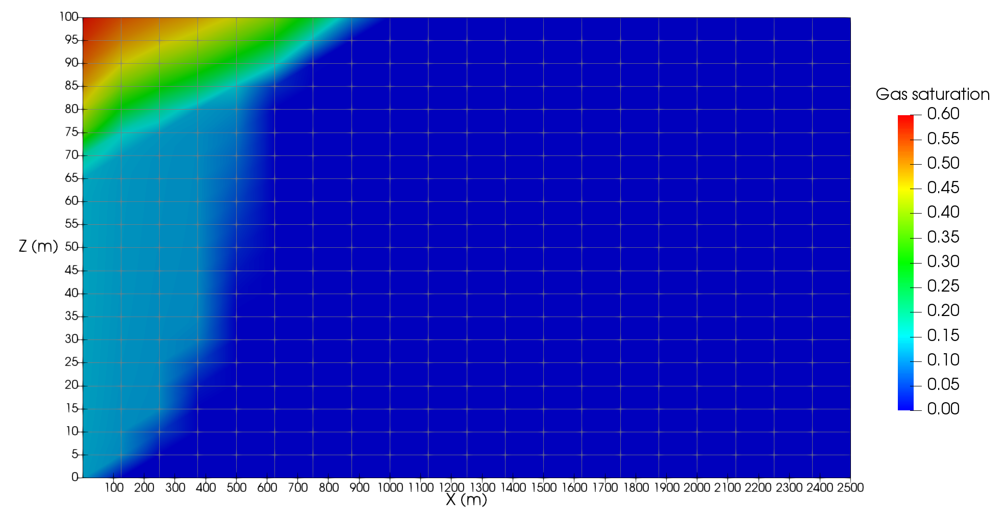
Figure 2: Gas saturation after 10 seconds
Due to the large density contrast between the injection methane (with a density of 175 kg m compared to approximately 1060 kg m), the methane migrates vertically and pools beneath the top of the reservoir, extending to a radial distance of approximately 900 m. Methane immobilised at residual saturation can be observed in the lower part of the reservoir (where the gas saturation is approximately 0.1).
Flexible restart using a SolutionUserObject
In the above example, the mesh used in the gas injection problem is initially identical to the mesh used in the gravity equilibrium run. MOOSE provides a more flexible restart capability where the mesh used in the subsequent simulation does not have to be identical to the mesh used in the initial simulation. Instead, the variable values from the initial simulation can be projected onto a new mesh in a subsequent simulation using a SolutionUserObject and SolutionFunction.
It is clear from the results shown above that the methane is expected near the upper left of the model (near the top of the injection well). We could refine the original mesh in that region using mesh adaptivity, but we instead construct a new mesh that is refined in that region and use a SolutionUserObject and SolutionFunction to project the initial value for liquid porepressure from the coarse gravity equilibrium mesh to the new mesh.
The input file for this example is
# Using the results from the equilibrium run to provide the initial condition for
# porepressure, we now inject a gas phase into the brine-saturated reservoir. In this
# example, the mesh is not identical to the mesh used in gravityeq.i. Rather, it is
# generated so that it is more refined near the injection boundary and at the top of
# the model, as that is where the gas plume will be present.
#
# To use the hydrostatic pressure calculated using the gravity equilibrium run as the initial
# condition for the pressure, a SolutionUserObject is used, along with a SolutionFunction to
# interpolate the pressure from the gravity equilibrium run to the initial condition for liqiud
# porepressure in this example.
#
# Even though the gravity equilibrium is established using a 2D mesh, in this example,
# we use a mesh shifted 0.1 m to the right and rotate it about the Y axis to make a 2D radial
# model.
#
# Methane injection takes place over the surface of the hole created by rotating the mesh,
# and hence the injection area is 2 pi r h. We can calculate this using an AreaPostprocessor,
# and then use this in a ParsedFunction to calculate the injection rate so that 10 kg/s of
# methane is injected.
#
# Note: as this example uses the results from a previous simulation, gravityeq.i MUST be
# run before running this input file.

[Mesh<<<{"href": "../../syntax/Mesh/index.html"}>>>]
  type = GeneratedMesh
  dim = 2
  ny = 25
  nx = 50
  ymax = 100
  xmin = 0.1
  xmax = 5000
  bias_x = 1.05
  bias_y = 0.95
  coord_type = RZ
  rz_coord_axis = Y
[]

[GlobalParams<<<{"href": "../../syntax/GlobalParams/index.html"}>>>]
  PorousFlowDictator = dictator
  gravity = '0 -9.81 0'
  temperature_unit = Celsius
[]

[Variables<<<{"href": "../../syntax/Variables/index.html"}>>>]
  [pp_liq]
  []
  [sat_gas]
    initial_condition<<<{"description": "Specifies a constant initial condition for this variable"}>>> = 0
  []
[]

[ICs<<<{"href": "../../syntax/ICs/index.html"}>>>]
  [ppliq_ic]
    type = FunctionIC<<<{"description": "An initial condition that uses a normal function of x, y, z to produce values (and optionally gradients) for a field variable.", "href": "../../source/ics/FunctionIC.html"}>>>
    variable<<<{"description": "The variable this initial condition is supposed to provide values for."}>>> = pp_liq
    function<<<{"description": "The initial condition function."}>>> = ppliq_ic
  []
[]

[AuxVariables<<<{"href": "../../syntax/AuxVariables/index.html"}>>>]
  [temperature]
    initial_condition<<<{"description": "Specifies a constant initial condition for this variable"}>>> = 50
  []
  [xnacl]
    initial_condition<<<{"description": "Specifies a constant initial condition for this variable"}>>> = 0.1
  []
  [brine_density]
    family<<<{"description": "Specifies the family of FE shape functions to use for this variable"}>>> = MONOMIAL
    order<<<{"description": "Specifies the order of the FE shape function to use for this variable (additional orders not listed are allowed)"}>>> = CONSTANT
  []
  [methane_density]
    family<<<{"description": "Specifies the family of FE shape functions to use for this variable"}>>> = MONOMIAL
    order<<<{"description": "Specifies the order of the FE shape function to use for this variable (additional orders not listed are allowed)"}>>> = CONSTANT
  []
  [massfrac_ph0_sp0]
    initial_condition<<<{"description": "Specifies a constant initial condition for this variable"}>>> = 1
  []
  [massfrac_ph1_sp0]
    initial_condition<<<{"description": "Specifies a constant initial condition for this variable"}>>> = 0
  []
  [pp_gas]
    family<<<{"description": "Specifies the family of FE shape functions to use for this variable"}>>> = MONOMIAL
    order<<<{"description": "Specifies the order of the FE shape function to use for this variable (additional orders not listed are allowed)"}>>> = CONSTANT
  []
  [sat_liq]
    family<<<{"description": "Specifies the family of FE shape functions to use for this variable"}>>> = MONOMIAL
    order<<<{"description": "Specifies the order of the FE shape function to use for this variable (additional orders not listed are allowed)"}>>> = CONSTANT
  []
[]

[Kernels<<<{"href": "../../syntax/Kernels/index.html"}>>>]
  [mass0]
    type = PorousFlowMassTimeDerivative<<<{"description": "Derivative of fluid-component mass with respect to time.  Mass lumping to the nodes is used.", "href": "../../source/kernels/PorousFlowMassTimeDerivative.html"}>>>
    variable<<<{"description": "The name of the variable that this residual object operates on"}>>> = pp_liq
  []
  [flux0]
    type = PorousFlowAdvectiveFlux<<<{"description": "Fully-upwinded advective flux of the component given by fluid_component", "href": "../../source/kernels/PorousFlowAdvectiveFlux.html"}>>>
    variable<<<{"description": "The name of the variable that this residual object operates on"}>>> = pp_liq
  []
  [mass1]
    type = PorousFlowMassTimeDerivative<<<{"description": "Derivative of fluid-component mass with respect to time.  Mass lumping to the nodes is used.", "href": "../../source/kernels/PorousFlowMassTimeDerivative.html"}>>>
    variable<<<{"description": "The name of the variable that this residual object operates on"}>>> = sat_gas
    fluid_component<<<{"description": "The index corresponding to the component for this kernel"}>>> = 1
  []
  [flux1]
    type = PorousFlowAdvectiveFlux<<<{"description": "Fully-upwinded advective flux of the component given by fluid_component", "href": "../../source/kernels/PorousFlowAdvectiveFlux.html"}>>>
    variable<<<{"description": "The name of the variable that this residual object operates on"}>>> = sat_gas
    fluid_component<<<{"description": "The index corresponding to the fluid component for this kernel"}>>> = 1
  []
[]

[AuxKernels<<<{"href": "../../syntax/AuxKernels/index.html"}>>>]
  [brine_density]
    type = PorousFlowPropertyAux<<<{"description": "AuxKernel to provide access to properties evaluated at quadpoints. Note that elemental AuxVariables must be used, so that these properties are integrated over each element.", "href": "../../source/auxkernels/PorousFlowPropertyAux.html"}>>>
    property<<<{"description": "The fluid property that this auxillary kernel is to calculate"}>>> = density
    variable<<<{"description": "The name of the variable that this object applies to"}>>> = brine_density
    execute_on<<<{"description": "The list of flag(s) indicating when this object should be executed. For a description of each flag, see https://mooseframework.inl.gov/source/interfaces/SetupInterface.html."}>>> = 'initial timestep_end'
  []
  [methane_density]
    type = PorousFlowPropertyAux<<<{"description": "AuxKernel to provide access to properties evaluated at quadpoints. Note that elemental AuxVariables must be used, so that these properties are integrated over each element.", "href": "../../source/auxkernels/PorousFlowPropertyAux.html"}>>>
    property<<<{"description": "The fluid property that this auxillary kernel is to calculate"}>>> = density
    variable<<<{"description": "The name of the variable that this object applies to"}>>> = methane_density
    phase<<<{"description": "The index of the phase this auxillary kernel acts on"}>>> = 1
    execute_on<<<{"description": "The list of flag(s) indicating when this object should be executed. For a description of each flag, see https://mooseframework.inl.gov/source/interfaces/SetupInterface.html."}>>> = 'initial timestep_end'
  []
  [pp_gas]
    type = PorousFlowPropertyAux<<<{"description": "AuxKernel to provide access to properties evaluated at quadpoints. Note that elemental AuxVariables must be used, so that these properties are integrated over each element.", "href": "../../source/auxkernels/PorousFlowPropertyAux.html"}>>>
    property<<<{"description": "The fluid property that this auxillary kernel is to calculate"}>>> = pressure
    phase<<<{"description": "The index of the phase this auxillary kernel acts on"}>>> = 1
    variable<<<{"description": "The name of the variable that this object applies to"}>>> = pp_gas
    execute_on<<<{"description": "The list of flag(s) indicating when this object should be executed. For a description of each flag, see https://mooseframework.inl.gov/source/interfaces/SetupInterface.html."}>>> = 'initial timestep_end'
  []
  [sat_liq]
    type = PorousFlowPropertyAux<<<{"description": "AuxKernel to provide access to properties evaluated at quadpoints. Note that elemental AuxVariables must be used, so that these properties are integrated over each element.", "href": "../../source/auxkernels/PorousFlowPropertyAux.html"}>>>
    property<<<{"description": "The fluid property that this auxillary kernel is to calculate"}>>> = saturation
    variable<<<{"description": "The name of the variable that this object applies to"}>>> = sat_liq
    execute_on<<<{"description": "The list of flag(s) indicating when this object should be executed. For a description of each flag, see https://mooseframework.inl.gov/source/interfaces/SetupInterface.html."}>>> = 'initial timestep_end'
  []
[]

[BCs<<<{"href": "../../syntax/BCs/index.html"}>>>]
  [gas_injection]
    type = PorousFlowSink<<<{"description": "Applies a flux sink to a boundary.", "href": "../../source/bcs/PorousFlowSink.html"}>>>
    boundary<<<{"description": "The list of boundary IDs from the mesh where this object applies"}>>> = left
    variable<<<{"description": "The name of the variable that this residual object operates on"}>>> = sat_gas
    flux_function<<<{"description": "The flux.  The flux is OUT of the medium: hence positive values of this function means this BC will act as a SINK, while negative values indicate this flux will be a SOURCE.  The functional form is useful for spatially or temporally varying sinks.  Without any use_*, this function is measured in kg.m^-2.s^-1 (or J.m^-2.s^-1 for the case with only heat and no fluids)"}>>> = injection_rate
    fluid_phase<<<{"description": "If supplied, then this BC will potentially be a function of fluid pressure, and you can use mass_fraction_component, use_mobility, use_relperm, use_enthalpy and use_energy.  If not supplied, then this BC can only be a function of temperature"}>>> = 1
  []
  [brine_out]
    type = PorousFlowPiecewiseLinearSink<<<{"description": "Applies a flux sink to a boundary. The base flux defined by PorousFlowSink is multiplied by a piecewise linear function.", "href": "../../source/bcs/PorousFlowPiecewiseLinearSink.html"}>>>
    boundary<<<{"description": "The list of boundary IDs from the mesh where this object applies"}>>> = right
    variable<<<{"description": "The name of the variable that this residual object operates on"}>>> = pp_liq
    multipliers<<<{"description": "Tuple of multiplying values.  The flux values are multiplied by these."}>>> = '0 1e9'
    pt_vals<<<{"description": "Tuple of pressure values (for the fluid_phase specified).  Must be monotonically increasing.  For heat fluxes that don't involve fluids, these are temperature values"}>>> = '0 1e9'
    fluid_phase<<<{"description": "If supplied, then this BC will potentially be a function of fluid pressure, and you can use mass_fraction_component, use_mobility, use_relperm, use_enthalpy and use_energy.  If not supplied, then this BC can only be a function of temperature"}>>> = 0
    flux_function<<<{"description": "The flux.  The flux is OUT of the medium: hence positive values of this function means this BC will act as a SINK, while negative values indicate this flux will be a SOURCE.  The functional form is useful for spatially or temporally varying sinks.  Without any use_*, this function is measured in kg.m^-2.s^-1 (or J.m^-2.s^-1 for the case with only heat and no fluids)"}>>> = 1e-6
    use_mobility<<<{"description": "If true, then fluxes are multiplied by (density*permeability_nn/viscosity), where the '_nn' indicates the component normal to the boundary.  In this case bare_flux is measured in Pa.m^-1.  This can be used in conjunction with other use_*"}>>> = true
    use_relperm<<<{"description": "If true, then fluxes are multiplied by relative permeability.  This can be used in conjunction with other use_*"}>>> = true
    mass_fraction_component<<<{"description": "The index corresponding to a fluid component.  If supplied, the flux will be multiplied by the nodal mass fraction for the component"}>>> = 0
  []
[]

[Functions<<<{"href": "../../syntax/Functions/index.html"}>>>]
  [injection_rate]
    type = ParsedFunction<<<{"description": "Function created by parsing a string", "href": "../../source/functions/MooseParsedFunction.html"}>>>
    symbol_values<<<{"description": "Constant numeric values, postprocessor names, function names, and scalar variables corresponding to the symbols in symbol_names."}>>> = injection_area
    symbol_names<<<{"description": "Symbols (excluding t,x,y,z) that are bound to the values provided by the corresponding items in the symbol_values vector."}>>> = area
    expression<<<{"description": "The user defined function."}>>> = '-1/area'
  []
  [ppliq_ic]
    type = SolutionFunction<<<{"description": "Function for reading a solution from file.", "href": "../../source/functions/SolutionFunction.html"}>>>
    solution<<<{"description": "The SolutionUserObject to extract data from."}>>> = soln
  []
[]

[UserObjects<<<{"href": "../../syntax/UserObjects/index.html"}>>>]
  [dictator]
    type = PorousFlowDictator<<<{"description": "Holds information on the PorousFlow variable names", "href": "../../source/userobjects/PorousFlowDictator.html"}>>>
    porous_flow_vars<<<{"description": "List of primary variables that are used in the PorousFlow simulation.  Jacobian entries involving derivatives wrt these variables will be computed.  In single-phase models you will just have one (eg 'pressure'), in two-phase models you will have two (eg 'p_water p_gas', or 'p_water s_water'), etc."}>>> = 'pp_liq sat_gas'
    number_fluid_phases<<<{"description": "The number of fluid phases in the simulation"}>>> = 2
    number_fluid_components<<<{"description": "The number of fluid components in the simulation"}>>> = 2
  []
  [pc]
    type = PorousFlowCapillaryPressureVG<<<{"description": "van Genuchten capillary pressure", "href": "../../source/userobjects/PorousFlowCapillaryPressureVG.html"}>>>
    alpha<<<{"description": "van Genuchten parameter alpha. Must be positive"}>>> = 1e-5
    m<<<{"description": "van Genuchten exponent m. Must be between 0 and 1, and optimally should be set to >0.5"}>>> = 0.5
    sat_lr<<<{"description": "Liquid residual saturation.  Must be between 0 and 1. Default is 0"}>>> = 0.2
    pc_max<<<{"description": "Maximum capillary pressure (Pa). Must be > 0. Default is 1e9"}>>> = 1e7
  []
  [soln]
    type = SolutionUserObject<<<{"description": "Reads a variable from a mesh in one simulation to another", "href": "../../source/userobjects/SolutionUserObject.html"}>>>
    mesh<<<{"description": "The name of the mesh file (must be xda/xdr, exodusII or nemesis file)."}>>> = gravityeq_out.e
    system_variables<<<{"description": "The name of the nodal and elemental variables from the file you want to use for values"}>>> = porepressure
  []
[]

[FluidProperties<<<{"href": "../../syntax/FluidProperties/index.html"}>>>]
  [brine]
    type = BrineFluidProperties<<<{"description": "Fluid properties for brine", "href": "../../source/fluidproperties/BrineFluidProperties.html"}>>>
  []
  [methane]
    type = MethaneFluidProperties<<<{"description": "Fluid properties for methane (CH4)", "href": "../../source/fluidproperties/MethaneFluidProperties.html"}>>>
  []
  [methane_tab]
    type = TabulatedBicubicFluidProperties<<<{"description": "Fluid properties using bicubic interpolation on tabulated values provided", "href": "../../source/fluidproperties/TabulatedBicubicFluidProperties.html"}>>>
    fp = methane
    save_file<<<{"description": "Whether to save the csv fluid properties file"}>>> = false
  []
[]

[Materials<<<{"href": "../../syntax/Materials/index.html"}>>>]
  [temperature]
    type = PorousFlowTemperature<<<{"description": "Material to provide temperature at the quadpoints or nodes and derivatives of it with respect to the PorousFlow variables", "href": "../../source/materials/PorousFlowTemperature.html"}>>>
    temperature<<<{"description": "Fluid temperature variable.  Note, the default is suitable if your simulation is using Kelvin units, but probably not for Celsius"}>>> = temperature
  []
  [ps]
    type = PorousFlow2PhasePS<<<{"description": "This Material calculates the 2 porepressures and the 2 saturations in a 2-phase situation, and derivatives of these with respect to the PorousFlowVariables.", "href": "../../source/materials/PorousFlow2PhasePS.html"}>>>
    phase0_porepressure<<<{"description": "Variable that is the porepressure of phase 0 (the liquid phase)"}>>> = pp_liq
    phase1_saturation<<<{"description": "Variable that is the saturation of phase 1 (the gas phase)"}>>> = sat_gas
    capillary_pressure<<<{"description": "Name of the UserObject defining the capillary pressure"}>>> = pc
  []
  [massfrac]
    type = PorousFlowMassFraction<<<{"description": "This Material forms a std::vector<std::vector ...> of mass-fractions out of the individual mass fractions", "href": "../../source/materials/PorousFlowMassFraction.html"}>>>
    mass_fraction_vars<<<{"description": "List of variables that represent the mass fractions.  Format is 'f_ph0^c0 f_ph0^c1 f_ph0^c2 ... f_ph0^c(N-2) f_ph1^c0 f_ph1^c1 fph1^c2 ... fph1^c(N-2) ... fphP^c0 f_phP^c1 fphP^c2 ... fphP^c(N-2)' where N=num_components and P=num_phases, and it is assumed that f_ph^c(N-1)=1-sum(f_ph^c,{c,0,N-2}) so that f_ph^c(N-1) need not be given.  If no variables are provided then num_phases=1=num_components."}>>> = 'massfrac_ph0_sp0 massfrac_ph1_sp0'
  []
  [brine]
    type = PorousFlowBrine<<<{"description": "This Material calculates fluid properties for brine at the quadpoints or nodes", "href": "../../source/materials/PorousFlowBrine.html"}>>>
    compute_enthalpy<<<{"description": "Compute the fluid enthalpy"}>>> = false
    compute_internal_energy<<<{"description": "Compute the fluid internal energy"}>>> = false
    xnacl<<<{"description": "The salt mass fraction in the brine (kg/kg)"}>>> = xnacl
    phase<<<{"description": "The phase number"}>>> = 0
  []
  [methane]
    type = PorousFlowSingleComponentFluid<<<{"description": "This Material calculates fluid properties at the quadpoints or nodes for a single component fluid", "href": "../../source/materials/PorousFlowSingleComponentFluid.html"}>>>
    compute_enthalpy<<<{"description": "Compute the fluid enthalpy"}>>> = false
    compute_internal_energy<<<{"description": "Compute the fluid internal energy"}>>> = false
    fp<<<{"description": "The name of the user object for fluid properties"}>>> = methane_tab
    phase<<<{"description": "The phase number"}>>> = 1
  []
  [porosity]
    type = PorousFlowPorosityConst<<<{"description": "This Material calculates the porosity assuming it is constant", "href": "../../source/materials/PorousFlowPorosityConst.html"}>>>
    porosity<<<{"description": "The porosity (assumed indepenent of porepressure, temperature, strain, etc, for this material).  This should be a real number, or a constant monomial variable (not a linear lagrange or other kind of variable)."}>>> = 0.1
  []
  [permeability]
    type = PorousFlowPermeabilityConst<<<{"description": "This Material calculates the permeability tensor assuming it is constant", "href": "../../source/materials/PorousFlowPermeabilityConst.html"}>>>
    permeability<<<{"description": "The permeability tensor (usually in m^2), which is assumed constant for this material"}>>> = '1e-13 0 0 0 5e-14 0  0 0 1e-13'
  []
  [relperm_liq]
    type = PorousFlowRelativePermeabilityCorey<<<{"description": "This Material calculates relative permeability of the fluid phase, using the simple Corey model ((S-S_res)/(1-sum(S_res)))^n", "href": "../../source/materials/PorousFlowRelativePermeabilityCorey.html"}>>>
    n<<<{"description": "The Corey exponent of the phase."}>>> = 2
    phase<<<{"description": "The phase number"}>>> = 0
    s_res<<<{"description": "The residual saturation of the phase j. Must be between 0 and 1"}>>> = 0.2
    sum_s_res<<<{"description": "Sum of residual saturations over all phases.  Must be between 0 and 1"}>>> = 0.3
  []
  [relperm_gas]
    type = PorousFlowRelativePermeabilityCorey<<<{"description": "This Material calculates relative permeability of the fluid phase, using the simple Corey model ((S-S_res)/(1-sum(S_res)))^n", "href": "../../source/materials/PorousFlowRelativePermeabilityCorey.html"}>>>
    n<<<{"description": "The Corey exponent of the phase."}>>> = 2
    phase<<<{"description": "The phase number"}>>> = 1
    s_res<<<{"description": "The residual saturation of the phase j. Must be between 0 and 1"}>>> = 0.1
    sum_s_res<<<{"description": "Sum of residual saturations over all phases.  Must be between 0 and 1"}>>> = 0.3
  []
[]

[Preconditioning<<<{"href": "../../syntax/Preconditioning/index.html"}>>>]
  [smp]
    type = SMP<<<{"description": "Single matrix preconditioner (SMP) builds a preconditioner using user defined off-diagonal parts of the Jacobian.", "href": "../../source/preconditioners/SingleMatrixPreconditioner.html"}>>>
    full<<<{"description": "Set to true if you want the full set of couplings between variables simply for convenience so you don't have to set every off_diag_row and off_diag_column combination."}>>> = true
    petsc_options_iname<<<{"description": "Names of PETSc name/value pairs"}>>> = '-pc_type -sub_pc_type -sub_pc_factor_shift_type'
    petsc_options_value<<<{"description": "Values of PETSc name/value pairs (must correspond with \"petsc_options_iname\""}>>> = ' asm      lu           NONZERO'
  []
[]

[Executioner<<<{"href": "../../syntax/Executioner/index.html"}>>>]
  type = Transient
  solve_type = Newton
  end_time = 1e8
  nl_abs_tol = 1e-12
  nl_rel_tol = 1e-06
  nl_max_its = 20
  dtmax = 1e6
  [TimeStepper<<<{"href": "../../syntax/Executioner/TimeStepper/index.html"}>>>]
    type = IterationAdaptiveDT
    dt = 1e1
    growth_factor = 1.5
  []
[]

[Postprocessors<<<{"href": "../../syntax/Postprocessors/index.html"}>>>]
  [mass_ph0]
    type = PorousFlowFluidMass<<<{"description": "Calculates the mass of a fluid component in a region", "href": "../../source/postprocessors/PorousFlowFluidMass.html"}>>>
    fluid_component<<<{"description": "The index corresponding to the fluid component that this Postprocessor acts on"}>>> = 0
    execute_on<<<{"description": "The list of flag(s) indicating when this object should be executed. For a description of each flag, see https://mooseframework.inl.gov/source/interfaces/SetupInterface.html."}>>> = 'initial timestep_end'
  []
  [mass_ph1]
    type = PorousFlowFluidMass<<<{"description": "Calculates the mass of a fluid component in a region", "href": "../../source/postprocessors/PorousFlowFluidMass.html"}>>>
    fluid_component<<<{"description": "The index corresponding to the fluid component that this Postprocessor acts on"}>>> = 1
    execute_on<<<{"description": "The list of flag(s) indicating when this object should be executed. For a description of each flag, see https://mooseframework.inl.gov/source/interfaces/SetupInterface.html."}>>> = 'initial timestep_end'
  []
  [injection_area]
    type = AreaPostprocessor<<<{"description": "Computes the \"area\" or dimension - 1 \"volume\" of a given boundary or boundaries in your mesh.", "href": "../../source/postprocessors/AreaPostprocessor.html"}>>>
    boundary<<<{"description": "The list of boundary IDs from the mesh where this object applies"}>>> = left
    execute_on<<<{"description": "The list of flag(s) indicating when this object should be executed. For a description of each flag, see https://mooseframework.inl.gov/source/interfaces/SetupInterface.html."}>>> = initial
  []
[]

[Outputs<<<{"href": "../../syntax/Outputs/index.html"}>>>]
  execute_on<<<{"description": "The list of flag(s) indicating when this object should be executed. For a description of each flag, see https://mooseframework.inl.gov/source/interfaces/SetupInterface.html."}>>> = 'initial timestep_end'
  exodus<<<{"description": "Output the results using the default settings for Exodus output."}>>> = true
  perf_graph<<<{"description": "Enable printing of the performance graph to the screen (Console)"}>>> = true
[]The mesh in this example is biased so that there are more elements in the upper left region, and fewer away from the well
[Mesh<<<{"href": "../../syntax/Mesh/index.html"}>>>]
  type = GeneratedMesh
  dim = 2
  ny = 25
  nx = 50
  ymax = 100
  xmin = 0.1
  xmax = 5000
  bias_x = 1.05
  bias_y = 0.95
  coord_type = RZ
  rz_coord_axis = Y
[]The results from the gravity equilibrium simulation are read using a SolutionUserObject
[UserObjects<<<{"href": "../../syntax/UserObjects/index.html"}>>>]
  [soln]
    type = SolutionUserObject<<<{"description": "Reads a variable from a mesh in one simulation to another", "href": "../../source/userobjects/SolutionUserObject.html"}>>>
    mesh<<<{"description": "The name of the mesh file (must be xda/xdr, exodusII or nemesis file)."}>>> = gravityeq_out.e
    system_variables<<<{"description": "The name of the nodal and elemental variables from the file you want to use for values"}>>> = porepressure
  []
[]A SolutionFunction is used to spatially interpolate these values
[Functions<<<{"href": "../../syntax/Functions/index.html"}>>>]
  [ppliq_ic]
    type = SolutionFunction<<<{"description": "Function for reading a solution from file.", "href": "../../source/functions/SolutionFunction.html"}>>>
    solution<<<{"description": "The SolutionUserObject to extract data from."}>>> = soln
  []
[]and finally a FunctionIC is used to set the initial condition of the liquid porepressure
[ICs<<<{"href": "../../syntax/ICs/index.html"}>>>]
  [ppliq_ic]
    type = FunctionIC<<<{"description": "An initial condition that uses a normal function of x, y, z to produce values (and optionally gradients) for a field variable.", "href": "../../source/ics/FunctionIC.html"}>>>
    variable<<<{"description": "The variable this initial condition is supposed to provide values for."}>>> = pp_liq
    function<<<{"description": "The initial condition function."}>>> = ppliq_ic
  []
[]This more refined model can then be run, resulting in the gas saturation profile shown in Figure 3.
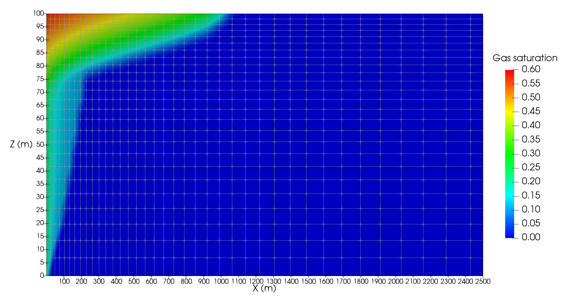
Figure 3: Gas saturation after 10 seconds
Due to the additional refinement near the well and the top of the reservoir, the gas saturation profile is now smoother near the well, with much less lateral migration in the lower part of the reservoir and hence much less methane immobilised at residual saturation. As a result, more methane is able to migrate to the top of the reservoir, and the lateral plume extends nearly 200 m further in this model than the coarser model shown above.
Generalisation to more complicated models
The above example of the restart capability demonstrates how PorousFlow can use the results of previous simulations as initial conditions of new simulations, even when changing from single-phase models to a more complex two-phase model. Of course, these approaches can be extended to models where heat and geomechanics are involved by setting initial conditions for additional variables using an identical approach to that demonstrated in this simple example.
Recovery
A simulation may fail prematurely due to external factors (such as exceeding the wall time on a cluster). In these cases a simulation may be recovered provided that checkpointing has been enabled.
[Outputs<<<{"href": "../../syntax/Outputs/index.html"}>>>]
  execute_on<<<{"description": "The list of flag(s) indicating when this object should be executed. For a description of each flag, see https://mooseframework.inl.gov/source/interfaces/SetupInterface.html."}>>> = 'initial timestep_end'
  exodus<<<{"description": "Output the results using the default settings for Exodus output."}>>> = true
  perf_graph<<<{"description": "Enable printing of the performance graph to the screen (Console)"}>>> = true
  checkpoint<<<{"description": "Create checkpoint files using the default options."}>>> = true
[]If the simulation gas_injection.i is interrupted for any reason, it may be recovered using the checkpoint data
porous_flow-opt -i gas_injection.i --recover
whereby the simulation will continue from the latest checkpoint data.
For this reason, it is strongly recommended that checkpointing is enabled in long-running jobs.