FluidFlower International Benchmark Study
Introduction
The FluidFlower International Benchmark Study was a collaborative effort at benchmarking numerical models of underground storate of CO using experimental results obtained with the FluidFlower experimental apparatus. The study was run by the University of Bergen, Norway, where the experiments were performed, with numerical modelling done by nine research groups worldwide.
FluidFlower experimental apparatus
The FluidFlower is a large, curved Hele-Shaw like apparatus where detailed and realistic geological models can be created. Pressure sensors are located at regular intervals, and optical characterisation of gas saturation and dissolution enable detailed experiemntal characterisation of the physical processes involved in geological storage of CO.
Numerical modelling study
The numerical models were developed without any access to the experimental results during the study. A full description of the problem is contained in Nordbotten et al. (2022). Participants initially developed their own models in the blind phase of the study, before comparing results amongst each other to enable groups to discuss important features. Finally, once each participant had submitted their final results, the experimental results were presented and compared to the numerical predictions. Full details are available in Flemisch et al. (2023).
MOOSE model
The Porous Flow module of MOOSE was used to model the FluidFlower experiments. Full details of the modelling is avaialble in Green et al. (2023), while a comparison to experiments is presented in Flemisch et al. (2023). As capillary barriers were a significant factor in the spatial distribution of CO, where gas saturation could be discontinuous between adjacent grid cells, the capability of the PorousFlow module was extended to use the finite volume method. This example serves as the first study using this new capability in the PorousFlow module.
A computational mesh was created using facies determined from high-resolution images of the exerimental apparatus, with petrophysical properties such as porosity and permeability assigned based on the values provided in Nordbotten et al. (2022), see Figure 1. Some important features to note are the (relatively) low permeability sealing units (dark blue facies), which also feature large capillary entry pressures. The lower sealing unit is bisected by a high permeability fault, so that CO would be expected to breach the sealing unit through this pathway. A second high-permeability fault is located in the upper right part of the model, while an impermeable seal (the white region) seperates the upper part of the reservoir.
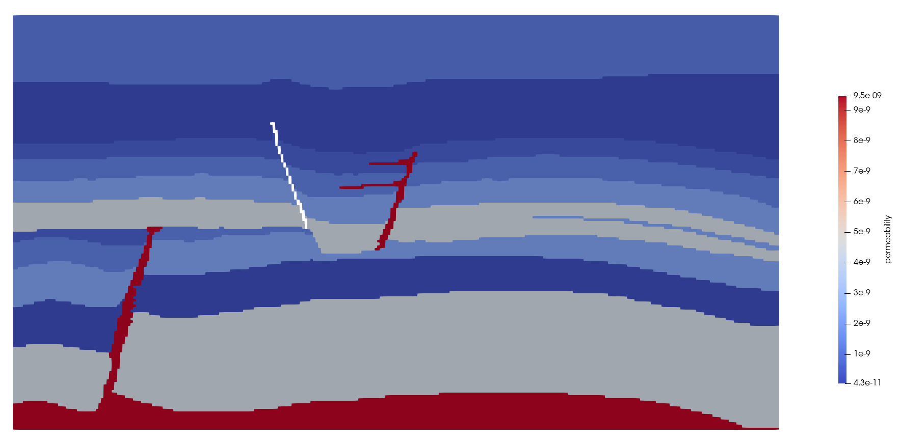
Figure 1: Permebility of each facies in the FluidFlower model
The input file that can be used to reproduce the results presented in Green et al. (2023) using MOOSE is rather lengthy and complicated, due to the different properties in each facies, the injection schedule, and the quantities that were required to be reported as part of the study. One important thing to note is that this problem is quite challenging numerically due to the large density contrast between the gas and liquid phases at ambient pressure and temperature conditions, which meant that extremely small timesteps had to be used in order for the nonlinear solver to converge. Consequently, this problem takes a long time to run (on the order of a day), and as it is only a 2D model with O(40K) cells only, it doesn't benefit significantly from parallelisation.
Nonetheless, this example does show how it is possible to describe a complicated heterogeneous model in MOOSE. Parameter substitution through input file variables (brace expresssions) are used extensivley to avoid possible errors in values. These are described in the comments at the top of the input file.
# FluidFlower International Benchmark study model
# CSIRO 2023
#
# This example can be used to reproduce the results presented by the
# CSIRO team as part of this benchmark study. See
# Green, C., Jackson, S.J., Gunning, J., Wilkins, A. and Ennis-King, J.,
# 2023. Modelling the FluidFlower: Insights from Characterisation and
# Numerical Predictions. Transport in Porous Media.
#
# This example takes a long time to run! The large density contrast
# between the gas phase CO2 and the water makes convergence very hard,
# so small timesteps must be taken during injection.
#
# This example uses a simplified mesh in order to be run during the
# automated testing. To reproduce the results of the benchmark study,
# replace the simple layered input mesh with the one located in the
# large_media submodule.
#
# The mesh file contains:
# - porosity as given by FluidFlower description
# - permeability as given by FluidFlower description
# - subdomain ids for each sand type
#
# The nominal thickness of the FluidFlower tank is 19mm. To keep masses consistent
# with the experiment, porosity and permeability are multiplied by the thickness
thickness = 0.019
#
# Properties associated with each sand type associated with mesh block ids
#
# block 0 - ESF (very fine sand)
sandESF = '0 10 20'
sandESF_pe = 1471.5
sandESF_krg = 0.09
sandESF_swi = 0.32
sandESF_krw = 0.71
sandESF_sgi = 0.14

# block 1 - C - Coarse lower
sandC = '1 21'
sandC_pe = 294.3
sandC_krg = 0.05
sandC_swi = 0.14
sandC_krw = 0.93
sandC_sgi = 0.1

# block 2 - D - Coarse upper
sandD = '2 22'
sandD_pe = 98.1
sandD_krg = 0.02
sandD_swi = 0.12
sandD_krw = 0.95
sandD_sgi = 0.08

# block 3 - E - Very Coarse lower
sandE = '3 13 23'
sandE_pe = 10
sandE_krg = 0.1
sandE_swi = 0.12
sandE_krw = 0.93
sandE_sgi = 0.06

# block 4 - F - Very Coarse upper
sandF = '4 14 24 34'
sandF_pe = 10
sandF_krg = 0.11
sandF_swi = 0.12
sandF_krw = 0.72
sandF_sgi = 0.13

# block 5 - G - Flush Zone
sandG = '5 15 35'
sandG_pe = 10
sandG_krg = 0.16
sandG_swi = 0.1
sandG_krw = 0.75
sandG_sgi = 0.06

# block 6 - Fault 1 - Heterogeneous
fault1 = '6 26'
fault1_pe = 10
fault1_krg = 0.16
fault1_swi = 0.1
fault1_krw = 0.75
fault1_sgi = 0.06

# block 7 - Fault 2 - Impermeable
# Note: this fault has been removed from the mesh (no elements in this region)

# block 8 - Fault 3 - Homogeneous
fault3 = '8'
fault3_pe = 10
fault3_krg = 0.16
fault3_swi = 0.1
fault3_krw = 0.75
fault3_sgi = 0.06

# Top layer
top_layer = '9'

# Boxes A, B an C used to report values (sg, sgr, xco2, etc)
boxA = '10 13 14 15 34 35'
boxB = '20 21 22 23 24 26'
boxC = '34 35'

# Furthermore, the seal sand unit in boxes A and B
seal_boxA = '10'
seal_boxB = '20'

# CO2 injection details:
# CO2 density ~1.8389 kg/m3 at 293.15 K, 1.01325e5 Pa
# Injection in Port (9, 3) for 5 hours.
# Injection in Port (17, 7) for 2:45 hours.
# Injection of 10 ml/min = 0.1666 ml/s = 1.666e-7 m3/s = ~3.06e-7 kg/s.
# Total mass of CO2 injected ~ 8.5g.
inj_rate = 3.06e-7The rest of the input file is typical of a PorousFlow input file.
Results
The MOOSE prediction of the spatial distribution of CO in each phase over the five days of the FluidFlower experiment are shown in Figure 2. In this figure, bright yellow represents CO in the gas phase, while lighter yellow represents CO dissolved in the water. During the two injection phases, CO is mainly in the gas phase. Due to the density contrast between the gas and liquid phases, the CO rapidly migrates upwards until it reaches a sealing unit (where the capillary entry pressure is greater than the gas pressure). It then fills these structural traps until they are full. As the lower structural trap becomes full, excess CO spills up the permeable fault in the bottom left of the model, migrating rapidly upwards until it reaches the next capillary barrier, where it spreads laterally again.
Figure 2: CO injection and dissolution in the FluidFlower geometry
As time continues, CO begins to dissolve into the water, increasing the liquid desnity slightly. This creates a gravitational instabilty, and results in convective mixing as evidenced by the complex downwelling fingers of CO saturated water. Dissolution continues until there is no CO in the gas phase at the end of the experiment.
Full details of the results obtained using MOOSE are presented in Green et al. (2023), while a comparison to the experimental results presented in Flemisch et al. (2023) show that the MOOSE predictions compared favourably to the experimental results.
References
- Bernd Flemisch, Jan M Nordbotten, Martin Fernø, Ruben Juanes, Holger Class, Mojdeh Delshad, Florian Doster, Jonathan Ennis-King, Jacques Franc, Sebastian Geiger, and others.
The FluidFlower Validation Benchmark Study for the Storage of CO$_2$.
Transport in Porous Media, pages 1–48, 2023.[Export]
- Christopher Green, Samuel J Jackson, James Gunning, Andy Wilkins, and Jonathan Ennis-King.
Modelling the fluidflower: insights from characterisation and numerical predictions.
Transport in Porous Media, pages 1–19, 2023.[Export]
- Jan M. Nordbotten, Martin Fernø, Bernd Flemisch, Ruben Juanes, and Magne Jørgensen.
Final Benchmark Description: FluidFlower International Benchmark Study.
July 2022.
URL: https://doi.org/10.5281/zenodo.6807102, doi:10.5281/zenodo.6807102.[Export]