Brine and carbon dioxide
The brine-CO model available in PorousFlow is a high precision equation of state for brine and CO, including the mutual solubility of CO into the liquid brine and water into the CO-rich gas phase. This model is suitable for simulations of geological storage of CO in saline aquifers, and is valid for temperatures in the range and pressures less than 60 MPa.
Salt (NaCl) can be included as a nonlinear variable, allowing salt to be transported along with water to provide variable density brine.
Phase composition
The mass fractions of CO in the liquid phase and HO in the gas phase are calculated using the accurate fugacity-based formulation of Spycher et al. (2003) and Spycher et al. (2005) for temperatures below 100C, and the elevated temperature formulation of Spycher and Pruess (2010) for temperatures above 110C.
As these formulations do not coincide for temperatures near 100C, a cubic polynomial is used to join the two curves smoothly, see Figure 1 for an example:
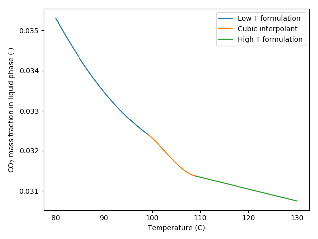
Figure 1: Dissolved CO mass fraction in brine versus temperature showing the low and high temperature formulations joined smoothly by a cubic polynomial. Results for pressure of 10 MPa and salt mass fraction of 0.01
The mutual solubilities in the elevated temperature regime must be calculated iteratively, so an increase in computational expense can be expected.
This is similar to the formulation provided in the ECO2N module of TOUGH2 (Pruess et al., 1999), see Figure 2 and Figure 3 for a comparison between the two codes.
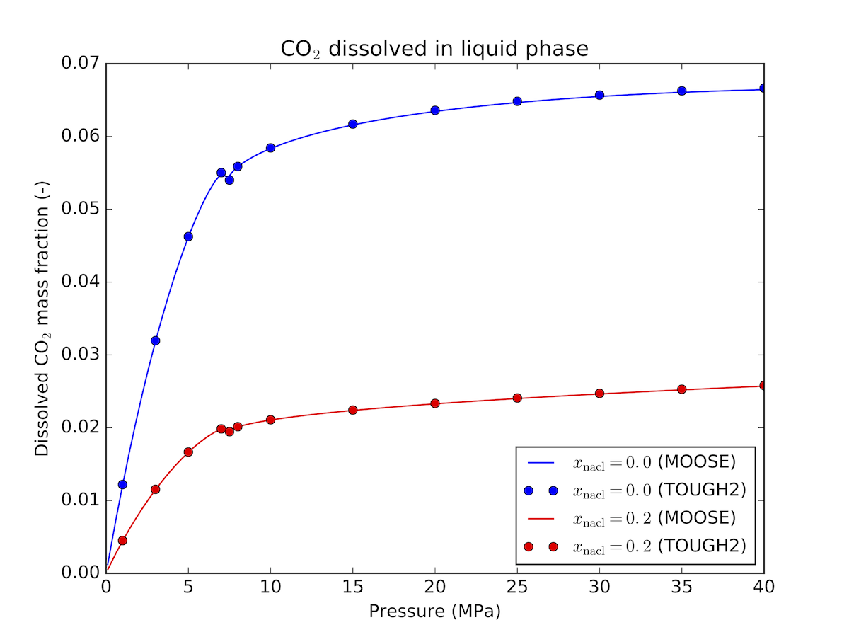
Figure 2: Dissolved CO mass fraction in brine - comparison between MOOSE and TOUGH2 at 30C
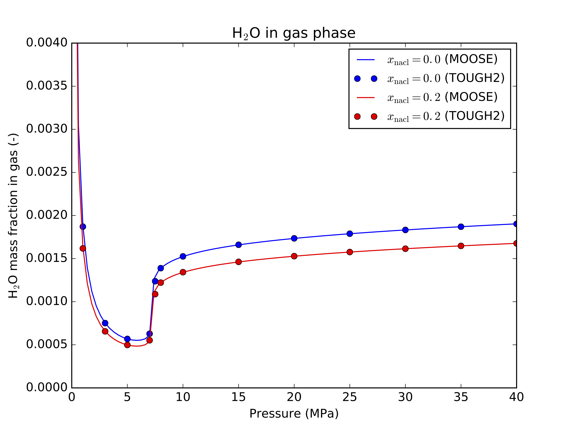
Figure 3: HO mass fraction in gas - comparison between MOOSE and TOUGH2 at 30C
As with many reservoir simulators, it is assumed that the phases are in instantaneous equilibrium, meaning that dissolution of CO into the brine and evaporation of water vapor into the CO phase happens instantaneously.
If the amount of CO present is not sufficient to saturate the brine, then no gas phase will be formed, and the dissolved CO mass fraction will be smaller than its equilibrium value. Similarly, if the amount of water vapor present is smaller than its equilibrium value in the gas phase, then no liquid phase can be formed.
If there is sufficient CO present to saturate the brine, then both liquid and gas phases will be present. In this case, the mass fraction of CO dissolved in the brine is given by its equilibrium value (for the current pressure, temperature and salinity). Similarly, the mass fraction of water vapor in the gas phase will be given by its equilibrium value in this two phase region.
Thermophysical properties
Density
The density of the aqueous phase with the contribution of dissolved CO is calculated using where is the density of brine (supplied using a BrineFluidProperties UserObject), is the mass fraction of CO dissolved in the aqueous phase, and is the partial density of dissolved CO (Garcia, 2001).
As water vapor is only ever a small component of the gas phase in the temperature and pressure ranges that this class is valid for, the density of the gas phase is assumed to be simply the density of CO at the given pressure and temperature, calculated using a CO2FluidProperties UserObject.
Viscosity
No contribution to the viscosity of each phase due to the presence of CO in the aqueous phase or water vapor in the gas phase is included. As a result, the viscosity of the aqueous phase is simply the viscosity of brine, while the viscosity of the gas phase is the viscosity of CO.
Enthalpy
The enthalpy of the gas phase is simply the enthalpy of CO at the given pressure and temperature values, with no contribution due to the presence of water vapor included.
The enthalpy of the liquid phase is also calculated as a weighted sum of the enthalpies of each individual component, but also includes a contribution due to the enthalpy of dissolution (a change in enthalpy due to dissolution of the NCG into the water phase) where is the enthalpy of brine, and is the enthalpy of CO in the liquid phase, which includes the enthalpy of dissolution
In the range of pressures and temperatures considered, CO may exist as a gas or a supercritical fluid. Using a linear fit to the model of Duan and Sun (2003), the enthalpy of dissolution of both gas phase and supercritical CO is calculated as
The calculation of brine and CO fluid properties can take a significant proportion of each simulation, so it is suggested that tabulated versions of both CO and brine properties are used using TabulatedFluidProperties.
Implementation
Variables
This class requires pressure of the gas phase, the total mass fraction of CO summed over all phases (see compositional flash for details), and the mass fraction of salt in the brine, for isothermal simulations. For nonisothermal simulations, temperature must also be provided as a nonlinear variable.
These variables must be listed as PorousFlow variables in the PorousFlowDictator UserObject
In the general isothermal case, three variables (gas porepressure, total CO mass fraction and salt mass fraction) are provided, one for each of the three possible fluid components (water, salt and CO). As a result, the number of components in the PorousFlowDictator must be set equal to three.
[UserObjects<<<{"href": "../../syntax/UserObjects/index.html"}>>>]
  [dictator]
    type = PorousFlowDictator<<<{"description": "Holds information on the PorousFlow variable names", "href": "../../source/userobjects/PorousFlowDictator.html"}>>>
    porous_flow_vars<<<{"description": "List of primary variables that are used in the PorousFlow simulation.  Jacobian entries involving derivatives wrt these variables will be computed.  In single-phase models you will just have one (eg 'pressure'), in two-phase models you will have two (eg 'p_water p_gas', or 'p_water s_water'), etc."}>>> = 'pgas zi xnacl'
    number_fluid_phases<<<{"description": "The number of fluid phases in the simulation"}>>> = 2
    number_fluid_components<<<{"description": "The number of fluid components in the simulation"}>>> = 3
  []
[]For nonisothermal cases, temperature must also be provided to ensure that all of the derivatives with respect to the temperature variable are calculated.
[UserObjects<<<{"href": "../../syntax/UserObjects/index.html"}>>>]
  [dictator]
    type = PorousFlowDictator<<<{"description": "Holds information on the PorousFlow variable names", "href": "../../source/userobjects/PorousFlowDictator.html"}>>>
    porous_flow_vars<<<{"description": "List of primary variables that are used in the PorousFlow simulation.  Jacobian entries involving derivatives wrt these variables will be computed.  In single-phase models you will just have one (eg 'pressure'), in two-phase models you will have two (eg 'p_water p_gas', or 'p_water s_water'), etc."}>>> = 'pgas zi xnacl temperature'
    number_fluid_phases<<<{"description": "The number of fluid phases in the simulation"}>>> = 2
    number_fluid_components<<<{"description": "The number of fluid components in the simulation"}>>> = 3
  []
[]Optionally, the salt mass fraction can be treated as a constant, in which case only gas porepressure and total CO mass fraction are required for the isothermal case, and the number of fluid components is two.
[UserObjects<<<{"href": "../../syntax/UserObjects/index.html"}>>>]
  [dictator]
    type = PorousFlowDictator<<<{"description": "Holds information on the PorousFlow variable names", "href": "../../source/userobjects/PorousFlowDictator.html"}>>>
    porous_flow_vars<<<{"description": "List of primary variables that are used in the PorousFlow simulation.  Jacobian entries involving derivatives wrt these variables will be computed.  In single-phase models you will just have one (eg 'pressure'), in two-phase models you will have two (eg 'p_water p_gas', or 'p_water s_water'), etc."}>>> = 'pgas z'
    number_fluid_phases<<<{"description": "The number of fluid phases in the simulation"}>>> = 2
    number_fluid_components<<<{"description": "The number of fluid components in the simulation"}>>> = 2
  []
[]UserObjects
This fluid state is implemented in the PorousFlowBrineCO2 UserObject. This UserObject is a GeneralUserObject that contains methods that provide a complete thermophysical description of the model given pressure, temperature and salt mass fraction.
[UserObjects<<<{"href": "../../syntax/UserObjects/index.html"}>>>]
  [fs]
    type = PorousFlowBrineCO2<<<{"description": "Fluid state class for brine and CO2", "href": "../../source/userobjects/PorousFlowBrineCO2.html"}>>>
    brine_fp<<<{"description": "The name of the user object for brine"}>>> = brine
    co2_fp<<<{"description": "The name of the user object for CO2"}>>> = co2
    capillary_pressure<<<{"description": "Name of the UserObject defining the capillary pressure"}>>> = pc
  []
[]Materials
The PorousFlowFluidState material provides all phase pressures, saturation, densities, viscosities etc, as well as all mass fractions of all fluid components in all fluid phases in a single material using the formulation provided in the PorousFlowBrineCO2 UserObject.
[Materials<<<{"href": "../../syntax/Materials/index.html"}>>>]
  [brineco2]
    type = PorousFlowFluidState<<<{"description": "Class for fluid state calculations using persistent primary variables and a vapor-liquid flash", "href": "../../source/materials/PorousFlowFluidState.html"}>>>
    gas_porepressure<<<{"description": "Variable that is the porepressure of the gas phase"}>>> = pgas
    z<<<{"description": "Total mass fraction of component i summed over all phases"}>>> = z
    temperature_unit<<<{"description": "The unit of the temperature variable"}>>> = Celsius
    xnacl<<<{"description": "The salt mass fraction in the brine (kg/kg)"}>>> = xnacl
    capillary_pressure<<<{"description": "Name of the UserObject defining the capillary pressure"}>>> = pc
    fluid_state<<<{"description": "Name of the FluidState UserObject"}>>> = fs
  []
[]For nonisothermal simulations, the temperature variable must also be supplied to ensure that all the derivatives with respect to the temperature variable are computed for the Jacobian.
[Materials<<<{"href": "../../syntax/Materials/index.html"}>>>]
  [brineco2]
    type = PorousFlowFluidState<<<{"description": "Class for fluid state calculations using persistent primary variables and a vapor-liquid flash", "href": "../../source/materials/PorousFlowFluidState.html"}>>>
    gas_porepressure<<<{"description": "Variable that is the porepressure of the gas phase"}>>> = pgas
    z<<<{"description": "Total mass fraction of component i summed over all phases"}>>> = zi
    temperature<<<{"description": "The fluid temperature (C or K, depending on temperature_unit)"}>>> = temperature
    temperature_unit<<<{"description": "The unit of the temperature variable"}>>> = Celsius
    xnacl<<<{"description": "The salt mass fraction in the brine (kg/kg)"}>>> = xnacl
    capillary_pressure<<<{"description": "Name of the UserObject defining the capillary pressure"}>>> = pc
    fluid_state<<<{"description": "Name of the FluidState UserObject"}>>> = fs
  []
[]Initial condition
The nonlinear variable representing CO is the total mass fraction of CO summed over all phases. In some cases, it may be preferred to provide an initial CO saturation, rather than total mass fraction. To allow an initial saturation to be specified, the PorousFlowFluidStateIC initial condition is provided. This initial condition calculates the total mass fraction of CO summed over all phases for a given saturation.
[ICs<<<{"href": "../../syntax/ICs/index.html"}>>>]
  [z]
    type = PorousFlowFluidStateIC<<<{"description": "An initial condition to calculate z from saturation", "href": "../../source/ics/PorousFlowFluidStateIC.html"}>>>
    saturation<<<{"description": "Gas saturation"}>>> = 0.5
    gas_porepressure<<<{"description": "Variable that is the porepressure of the gas phase"}>>> = pgas
    temperature<<<{"description": "Variable that is the fluid temperature"}>>> = 50
    variable<<<{"description": "The variable this initial condition is supposed to provide values for."}>>> = z
    xnacl<<<{"description": "The salt mass fraction in the brine (kg/kg)"}>>> = 0.1
    fluid_state<<<{"description": "Name of the FluidState UserObject"}>>> = fs
  []
[]Example
1D Radial injection
Injection into a one dimensional radial reservoir is a useful test of this class, as it admits a similarity solution , where is the radial distance from the injection well, and is time. This similarity solution holds even when complicated physics such as mutual solubility is included.
An example of a 1D radial injection problem is included in the test suite.
# Two phase Theis problem: Flow from single source.
# Constant rate injection 2 kg/s
# 1D cylindrical mesh
# Initially, system has only a liquid phase, until enough gas is injected
# to form a gas phase, in which case the system becomes two phase.
#
# This test takes a few minutes to run, so is marked heavy

[Mesh<<<{"href": "../../syntax/Mesh/index.html"}>>>]
  type = GeneratedMesh
  dim = 1
  nx = 2000
  xmax = 2000
  rz_coord_axis = Y
  coord_type = RZ
[]

[Problem<<<{"href": "../../syntax/Problem/index.html"}>>>]
  type = FEProblem
[]

[GlobalParams<<<{"href": "../../syntax/GlobalParams/index.html"}>>>]
  PorousFlowDictator = dictator
  gravity = '0 0 0'
[]

[AuxVariables<<<{"href": "../../syntax/AuxVariables/index.html"}>>>]
  [saturation_gas]
    order<<<{"description": "Specifies the order of the FE shape function to use for this variable (additional orders not listed are allowed)"}>>> = CONSTANT
    family<<<{"description": "Specifies the family of FE shape functions to use for this variable"}>>> = MONOMIAL
  []
  [x1]
    order<<<{"description": "Specifies the order of the FE shape function to use for this variable (additional orders not listed are allowed)"}>>> = CONSTANT
    family<<<{"description": "Specifies the family of FE shape functions to use for this variable"}>>> = MONOMIAL
  []
  [y0]
    order<<<{"description": "Specifies the order of the FE shape function to use for this variable (additional orders not listed are allowed)"}>>> = CONSTANT
    family<<<{"description": "Specifies the family of FE shape functions to use for this variable"}>>> = MONOMIAL
  []
[]

[AuxKernels<<<{"href": "../../syntax/AuxKernels/index.html"}>>>]
  [saturation_gas]
    type = PorousFlowPropertyAux<<<{"description": "AuxKernel to provide access to properties evaluated at quadpoints. Note that elemental AuxVariables must be used, so that these properties are integrated over each element.", "href": "../../source/auxkernels/PorousFlowPropertyAux.html"}>>>
    variable<<<{"description": "The name of the variable that this object applies to"}>>> = saturation_gas
    property<<<{"description": "The fluid property that this auxillary kernel is to calculate"}>>> = saturation
    phase<<<{"description": "The index of the phase this auxillary kernel acts on"}>>> = 1
    execute_on<<<{"description": "The list of flag(s) indicating when this object should be executed. For a description of each flag, see https://mooseframework.inl.gov/source/interfaces/SetupInterface.html."}>>> = timestep_end
  []
  [x1]
    type = PorousFlowPropertyAux<<<{"description": "AuxKernel to provide access to properties evaluated at quadpoints. Note that elemental AuxVariables must be used, so that these properties are integrated over each element.", "href": "../../source/auxkernels/PorousFlowPropertyAux.html"}>>>
    variable<<<{"description": "The name of the variable that this object applies to"}>>> = x1
    property<<<{"description": "The fluid property that this auxillary kernel is to calculate"}>>> = mass_fraction
    phase<<<{"description": "The index of the phase this auxillary kernel acts on"}>>> = 0
    fluid_component<<<{"description": "The index of the fluid component this auxillary kernel acts on"}>>> = 1
    execute_on<<<{"description": "The list of flag(s) indicating when this object should be executed. For a description of each flag, see https://mooseframework.inl.gov/source/interfaces/SetupInterface.html."}>>> = timestep_end
  []
  [y0]
    type = PorousFlowPropertyAux<<<{"description": "AuxKernel to provide access to properties evaluated at quadpoints. Note that elemental AuxVariables must be used, so that these properties are integrated over each element.", "href": "../../source/auxkernels/PorousFlowPropertyAux.html"}>>>
    variable<<<{"description": "The name of the variable that this object applies to"}>>> = y0
    property<<<{"description": "The fluid property that this auxillary kernel is to calculate"}>>> = mass_fraction
    phase<<<{"description": "The index of the phase this auxillary kernel acts on"}>>> = 1
    fluid_component<<<{"description": "The index of the fluid component this auxillary kernel acts on"}>>> = 0
    execute_on<<<{"description": "The list of flag(s) indicating when this object should be executed. For a description of each flag, see https://mooseframework.inl.gov/source/interfaces/SetupInterface.html."}>>> = timestep_end
  []
[]

[Variables<<<{"href": "../../syntax/Variables/index.html"}>>>]
  [pgas]
    initial_condition<<<{"description": "Specifies a constant initial condition for this variable"}>>> = 20e6
  []
  [zi]
    initial_condition<<<{"description": "Specifies a constant initial condition for this variable"}>>> = 0
  []
  [xnacl]
    initial_condition<<<{"description": "Specifies a constant initial condition for this variable"}>>> = 0.1
  []
[]

[Kernels<<<{"href": "../../syntax/Kernels/index.html"}>>>]
  [mass0]
    type = PorousFlowMassTimeDerivative<<<{"description": "Derivative of fluid-component mass with respect to time.  Mass lumping to the nodes is used.", "href": "../../source/kernels/PorousFlowMassTimeDerivative.html"}>>>
    fluid_component<<<{"description": "The index corresponding to the component for this kernel"}>>> = 0
    variable<<<{"description": "The name of the variable that this residual object operates on"}>>> = pgas
  []
  [flux0]
    type = PorousFlowAdvectiveFlux<<<{"description": "Fully-upwinded advective flux of the component given by fluid_component", "href": "../../source/kernels/PorousFlowAdvectiveFlux.html"}>>>
    fluid_component<<<{"description": "The index corresponding to the fluid component for this kernel"}>>> = 0
    variable<<<{"description": "The name of the variable that this residual object operates on"}>>> = pgas
  []
  [mass1]
    type = PorousFlowMassTimeDerivative<<<{"description": "Derivative of fluid-component mass with respect to time.  Mass lumping to the nodes is used.", "href": "../../source/kernels/PorousFlowMassTimeDerivative.html"}>>>
    fluid_component<<<{"description": "The index corresponding to the component for this kernel"}>>> = 1
    variable<<<{"description": "The name of the variable that this residual object operates on"}>>> = zi
  []
  [flux1]
    type = PorousFlowAdvectiveFlux<<<{"description": "Fully-upwinded advective flux of the component given by fluid_component", "href": "../../source/kernels/PorousFlowAdvectiveFlux.html"}>>>
    fluid_component<<<{"description": "The index corresponding to the fluid component for this kernel"}>>> = 1
    variable<<<{"description": "The name of the variable that this residual object operates on"}>>> = zi
  []
  [mass2]
    type = PorousFlowMassTimeDerivative<<<{"description": "Derivative of fluid-component mass with respect to time.  Mass lumping to the nodes is used.", "href": "../../source/kernels/PorousFlowMassTimeDerivative.html"}>>>
    fluid_component<<<{"description": "The index corresponding to the component for this kernel"}>>> = 2
    variable<<<{"description": "The name of the variable that this residual object operates on"}>>> = xnacl
  []
  [flux2]
    type = PorousFlowAdvectiveFlux<<<{"description": "Fully-upwinded advective flux of the component given by fluid_component", "href": "../../source/kernels/PorousFlowAdvectiveFlux.html"}>>>
    fluid_component<<<{"description": "The index corresponding to the fluid component for this kernel"}>>> = 2
    variable<<<{"description": "The name of the variable that this residual object operates on"}>>> = xnacl
  []
[]

[UserObjects<<<{"href": "../../syntax/UserObjects/index.html"}>>>]
  [dictator]
    type = PorousFlowDictator<<<{"description": "Holds information on the PorousFlow variable names", "href": "../../source/userobjects/PorousFlowDictator.html"}>>>
    porous_flow_vars<<<{"description": "List of primary variables that are used in the PorousFlow simulation.  Jacobian entries involving derivatives wrt these variables will be computed.  In single-phase models you will just have one (eg 'pressure'), in two-phase models you will have two (eg 'p_water p_gas', or 'p_water s_water'), etc."}>>> = 'pgas zi xnacl'
    number_fluid_phases<<<{"description": "The number of fluid phases in the simulation"}>>> = 2
    number_fluid_components<<<{"description": "The number of fluid components in the simulation"}>>> = 3
  []
  [pc]
    type = PorousFlowCapillaryPressureConst<<<{"description": "Constant capillary pressure", "href": "../../source/userobjects/PorousFlowCapillaryPressureConst.html"}>>>
    pc<<<{"description": "Constant capillary pressure (Pa). Default is 0"}>>> = 0
  []
  [fs]
    type = PorousFlowBrineCO2<<<{"description": "Fluid state class for brine and CO2", "href": "../../source/userobjects/PorousFlowBrineCO2.html"}>>>
    brine_fp<<<{"description": "The name of the user object for brine"}>>> = brine
    co2_fp<<<{"description": "The name of the user object for CO2"}>>> = co2
    capillary_pressure<<<{"description": "Name of the UserObject defining the capillary pressure"}>>> = pc
  []
[]

[FluidProperties<<<{"href": "../../syntax/FluidProperties/index.html"}>>>]
  [co2sw]
    type = CO2FluidProperties<<<{"description": "Fluid properties for carbon dioxide (CO2) using the Span & Wagner EOS", "href": "../../source/fluidproperties/CO2FluidProperties.html"}>>>
  []
  [co2]
    type = TabulatedFluidProperties<<<{"description": "Fluid properties using bicubic interpolation on tabulated values provided", "href": "../../source/fluidproperties/TabulatedBicubicFluidProperties.html"}>>>
    fp = co2sw
    fluid_property_file<<<{"description": "Name of the csv file containing the tabulated fluid property data."}>>> = 'fluid_properties.csv'
    allow_fp_and_tabulation<<<{"description": "Whether to allow the two sources of data concurrently"}>>> = true
    error_on_out_of_bounds<<<{"description": "Whether pressure or temperature from tabulation exceeding user-specified bounds leads to an error."}>>> = false
  []
  [water]
    type = Water97FluidProperties<<<{"description": "Fluid properties for water and steam (H2O) using IAPWS-IF97", "href": "../../source/fluidproperties/Water97FluidProperties.html"}>>>
  []
  [watertab]
    type = TabulatedFluidProperties<<<{"description": "Fluid properties using bicubic interpolation on tabulated values provided", "href": "../../source/fluidproperties/TabulatedBicubicFluidProperties.html"}>>>
    fp = water
    temperature_min<<<{"description": "Minimum temperature for tabulated data."}>>> = 273.15
    temperature_max<<<{"description": "Maximum temperature for tabulated data."}>>> = 573.15
    fluid_property_output_file<<<{"description": "Name of the CSV file which can be output with the tabulation. This file can then be read as a 'fluid_property_file'"}>>> = water_fluid_properties.csv
    # Comment out the fp parameter and uncomment below to use the newly generated tabulation
    # fluid_property_file = water_fluid_properties.csv
  []
  [brine]
    type = BrineFluidProperties<<<{"description": "Fluid properties for brine", "href": "../../source/fluidproperties/BrineFluidProperties.html"}>>>
    water_fp<<<{"description": "The name of the FluidProperties UserObject for water"}>>> = watertab
  []
[]

[Materials<<<{"href": "../../syntax/Materials/index.html"}>>>]
  [temperature]
    type = PorousFlowTemperature<<<{"description": "Material to provide temperature at the quadpoints or nodes and derivatives of it with respect to the PorousFlow variables", "href": "../../source/materials/PorousFlowTemperature.html"}>>>
    temperature<<<{"description": "Fluid temperature variable.  Note, the default is suitable if your simulation is using Kelvin units, but probably not for Celsius"}>>> = 20
  []
  [brineco2]
    type = PorousFlowFluidState<<<{"description": "Class for fluid state calculations using persistent primary variables and a vapor-liquid flash", "href": "../../source/materials/PorousFlowFluidState.html"}>>>
    gas_porepressure<<<{"description": "Variable that is the porepressure of the gas phase"}>>> = pgas
    z<<<{"description": "Total mass fraction of component i summed over all phases"}>>> = zi
    temperature_unit<<<{"description": "The unit of the temperature variable"}>>> = Celsius
    xnacl<<<{"description": "The salt mass fraction in the brine (kg/kg)"}>>> = xnacl
    capillary_pressure<<<{"description": "Name of the UserObject defining the capillary pressure"}>>> = pc
    fluid_state<<<{"description": "Name of the FluidState UserObject"}>>> = fs
  []
  [porosity]
    type = PorousFlowPorosityConst<<<{"description": "This Material calculates the porosity assuming it is constant", "href": "../../source/materials/PorousFlowPorosityConst.html"}>>>
    porosity<<<{"description": "The porosity (assumed indepenent of porepressure, temperature, strain, etc, for this material).  This should be a real number, or a constant monomial variable (not a linear lagrange or other kind of variable)."}>>> = 0.2
  []
  [permeability]
    type = PorousFlowPermeabilityConst<<<{"description": "This Material calculates the permeability tensor assuming it is constant", "href": "../../source/materials/PorousFlowPermeabilityConst.html"}>>>
    permeability<<<{"description": "The permeability tensor (usually in m^2), which is assumed constant for this material"}>>> = '1e-12 0 0 0 1e-12 0 0 0 1e-12'
  []
  [relperm_water]
    type = PorousFlowRelativePermeabilityCorey<<<{"description": "This Material calculates relative permeability of the fluid phase, using the simple Corey model ((S-S_res)/(1-sum(S_res)))^n", "href": "../../source/materials/PorousFlowRelativePermeabilityCorey.html"}>>>
    n<<<{"description": "The Corey exponent of the phase."}>>> = 2
    phase<<<{"description": "The phase number"}>>> = 0
    s_res<<<{"description": "The residual saturation of the phase j. Must be between 0 and 1"}>>> = 0.1
    sum_s_res<<<{"description": "Sum of residual saturations over all phases.  Must be between 0 and 1"}>>> = 0.1
  []
  [relperm_gas]
    type = PorousFlowRelativePermeabilityCorey<<<{"description": "This Material calculates relative permeability of the fluid phase, using the simple Corey model ((S-S_res)/(1-sum(S_res)))^n", "href": "../../source/materials/PorousFlowRelativePermeabilityCorey.html"}>>>
    n<<<{"description": "The Corey exponent of the phase."}>>> = 2
    phase<<<{"description": "The phase number"}>>> = 1
  []
[]

[BCs<<<{"href": "../../syntax/BCs/index.html"}>>>]
  [rightwater]
    type = DirichletBC<<<{"description": "Imposes the essential boundary condition $u=g$, where $g$ is a constant, controllable value.", "href": "../../source/bcs/DirichletBC.html"}>>>
    boundary<<<{"description": "The list of boundary IDs from the mesh where this object applies"}>>> = right
    value<<<{"description": "Value of the BC"}>>> = 20e6
    variable<<<{"description": "The name of the variable that this residual object operates on"}>>> = pgas
  []
[]

[DiracKernels<<<{"href": "../../syntax/DiracKernels/index.html"}>>>]
  [source]
    type = PorousFlowSquarePulsePointSource<<<{"description": "Point source (or sink) that adds (removes) fluid at a constant mass flux rate for times between the specified start and end times.", "href": "../../source/dirackernels/PorousFlowSquarePulsePointSource.html"}>>>
    point<<<{"description": "The x,y,z coordinates of the point source (sink)"}>>> = '0 0 0'
    mass_flux<<<{"description": "The mass flux at this point in kg/s (positive is flux in, negative is flux out)"}>>> = 2
    variable<<<{"description": "The name of the variable that this residual object operates on"}>>> = zi
  []
[]

[Preconditioning<<<{"href": "../../syntax/Preconditioning/index.html"}>>>]
  [smp]
    type = SMP<<<{"description": "Single matrix preconditioner (SMP) builds a preconditioner using user defined off-diagonal parts of the Jacobian.", "href": "../../source/preconditioners/SingleMatrixPreconditioner.html"}>>>
    full<<<{"description": "Set to true if you want the full set of couplings between variables simply for convenience so you don't have to set every off_diag_row and off_diag_column combination."}>>> = true
  []
[]

[Executioner<<<{"href": "../../syntax/Executioner/index.html"}>>>]
  type = Transient
  solve_type = NEWTON
  end_time = 1e5
  [TimeStepper<<<{"href": "../../syntax/Executioner/TimeStepper/index.html"}>>>]
    type = IterationAdaptiveDT
    dt = 1
    growth_factor = 1.5
  []
[]

[VectorPostprocessors<<<{"href": "../../syntax/VectorPostprocessors/index.html"}>>>]
  [line]
    type = LineValueSampler<<<{"description": "Samples variable(s) along a specified line", "href": "../../source/vectorpostprocessors/LineValueSampler.html"}>>>
    warn_discontinuous_face_values<<<{"description": "Whether to return a warning if a discontinuous variable is sampled on a face"}>>> = false
    sort_by<<<{"description": "What to sort the samples by. Options include 'x', 'y', 'z', 'id', and the name of any of the sampled quantities (which each create a vector of the same name)."}>>> = x
    start_point<<<{"description": "The beginning of the line"}>>> = '0 0 0'
    end_point<<<{"description": "The ending of the line"}>>> = '2000 0 0'
    num_points<<<{"description": "The number of points to sample along the line"}>>> = 10000
    variable<<<{"description": "The names of the variables that this VectorPostprocessor operates on"}>>> = 'pgas zi xnacl x1 saturation_gas'
    execute_on<<<{"description": "The list of flag(s) indicating when this object should be executed. For a description of each flag, see https://mooseframework.inl.gov/source/interfaces/SetupInterface.html."}>>> = 'timestep_end'
  []
[]

[Postprocessors<<<{"href": "../../syntax/Postprocessors/index.html"}>>>]
  [pgas]
    type = PointValue<<<{"description": "Compute the value of a variable at a specified location", "href": "../../source/postprocessors/PointValue.html"}>>>
    point<<<{"description": "The physical point where the solution will be evaluated."}>>> = '4 0 0'
    variable<<<{"description": "The name of the variable that this postprocessor operates on."}>>> = pgas
  []
  [sgas]
    type = PointValue<<<{"description": "Compute the value of a variable at a specified location", "href": "../../source/postprocessors/PointValue.html"}>>>
    point<<<{"description": "The physical point where the solution will be evaluated."}>>> = '4 0 0'
    variable<<<{"description": "The name of the variable that this postprocessor operates on."}>>> = saturation_gas
  []
  [zi]
    type = PointValue<<<{"description": "Compute the value of a variable at a specified location", "href": "../../source/postprocessors/PointValue.html"}>>>
    point<<<{"description": "The physical point where the solution will be evaluated."}>>> = '4 0 0'
    variable<<<{"description": "The name of the variable that this postprocessor operates on."}>>> = zi
  []
  [massgas]
    type = PorousFlowFluidMass<<<{"description": "Calculates the mass of a fluid component in a region", "href": "../../source/postprocessors/PorousFlowFluidMass.html"}>>>
    fluid_component<<<{"description": "The index corresponding to the fluid component that this Postprocessor acts on"}>>> = 1
  []
  [x1]
    type = PointValue<<<{"description": "Compute the value of a variable at a specified location", "href": "../../source/postprocessors/PointValue.html"}>>>
    point<<<{"description": "The physical point where the solution will be evaluated."}>>> = '4 0 0'
    variable<<<{"description": "The name of the variable that this postprocessor operates on."}>>> = x1
  []
  [y0]
    type = PointValue<<<{"description": "Compute the value of a variable at a specified location", "href": "../../source/postprocessors/PointValue.html"}>>>
    point<<<{"description": "The physical point where the solution will be evaluated."}>>> = '4 0 0'
    variable<<<{"description": "The name of the variable that this postprocessor operates on."}>>> = y0
  []
  [xnacl]
    type = PointValue<<<{"description": "Compute the value of a variable at a specified location", "href": "../../source/postprocessors/PointValue.html"}>>>
    point<<<{"description": "The physical point where the solution will be evaluated."}>>> = '4 0 0'
    variable<<<{"description": "The name of the variable that this postprocessor operates on."}>>> = xnacl
  []
[]

[Outputs<<<{"href": "../../syntax/Outputs/index.html"}>>>]
  print_linear_residuals<<<{"description": "Enable printing of linear residuals to the screen (Console)"}>>> = false
  perf_graph<<<{"description": "Enable printing of the performance graph to the screen (Console)"}>>> = true
  [csvout]
    type = CSV<<<{"description": "Output for postprocessors, vector postprocessors, and scalar variables using comma seperated values (CSV).", "href": "../../source/outputs/CSV.html"}>>>
    execute_on<<<{"description": "The list of flag(s) indicating when this object should be executed. For a description of each flag, see https://mooseframework.inl.gov/source/interfaces/SetupInterface.html."}>>> = timestep_end
    execute_vector_postprocessors_on<<<{"description": "Enable/disable the output of VectorPostprocessors"}>>> = final
  []
[]Initially, all of the CO injected is dissolved in the resident brine, as the amount of CO is less than the dissolved mass fraction at equilibrium. After a while, the brine near the injection well becomes saturated with CO, and a gas phase forms. This gas phase then spreads radially as injection continues. The mass fraction of salt in the brine decreases slightly where CO is present, due to the increased density of the brine following dissolution of CO.
A comparison of the results expressed in terms of the similarity solution is presented in Figure 4 for all three nonlinear variables for the case where is fixed (evaluated using Postprocessors), and also the case where is fixed (evaluated using a VectorPostprocessor).
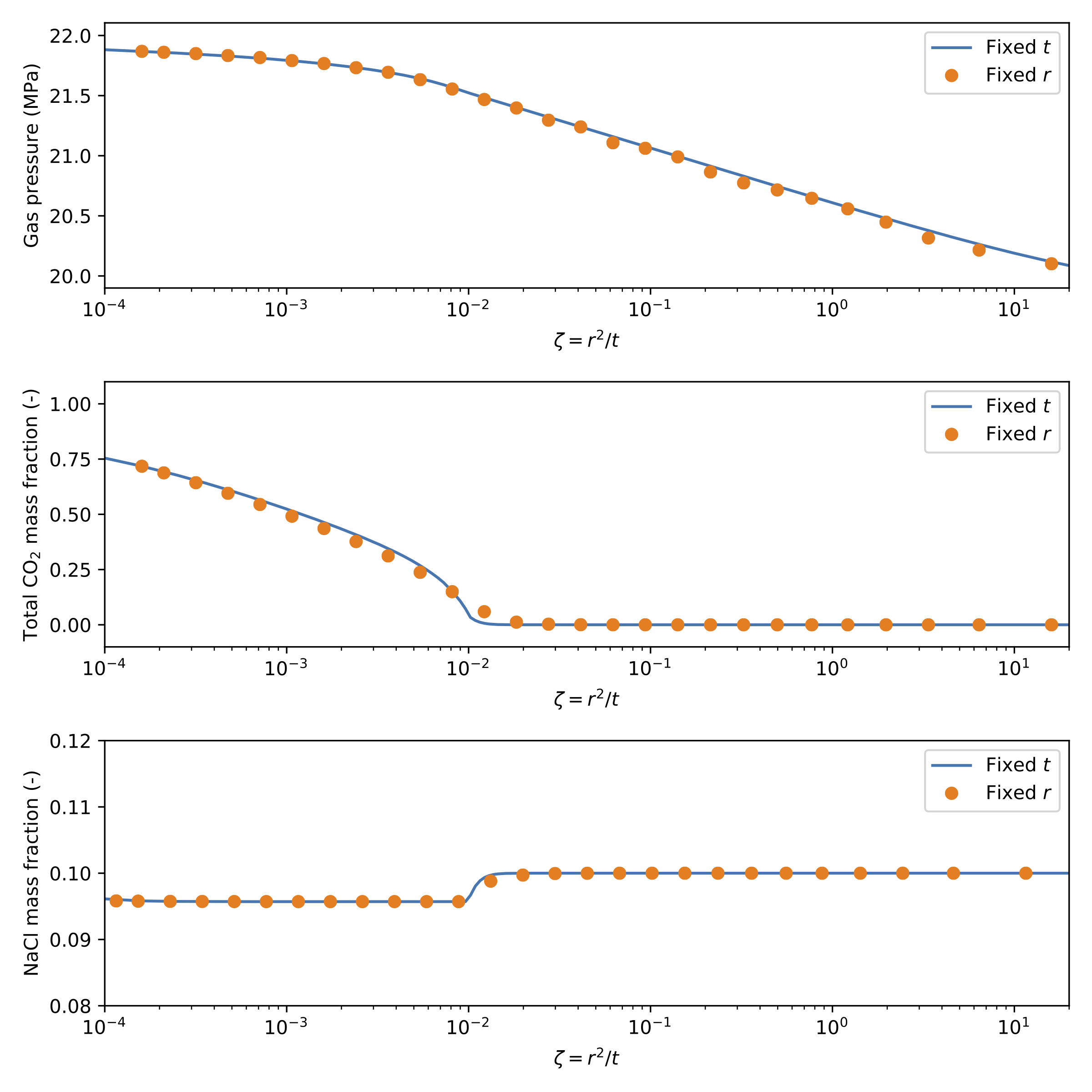
Figure 4: Similarity solution for 1D radial injection example
As these results show, the similarity solution holds for this problem.
An nonisothermal example of the above problem, where cold CO is injected into a warm aquifer, is also provided in the test suite.
# Two phase nonisothermal Theis problem: Flow from single source.
# Constant rate injection 2 kg/s of cold CO2 into warm reservoir
# 1D cylindrical mesh
# Initially, system has only a liquid phase, until enough gas is injected
# to form a gas phase, in which case the system becomes two phase.

[Mesh<<<{"href": "../../syntax/Mesh/index.html"}>>>]
  [mesh]
    type = GeneratedMeshGenerator<<<{"description": "Create a line, square, or cube mesh with uniformly spaced or biased elements.", "href": "../../source/meshgenerators/GeneratedMeshGenerator.html"}>>>
    dim<<<{"description": "The dimension of the mesh to be generated"}>>> = 1
    nx<<<{"description": "Number of elements in the X direction"}>>> = 40
    xmin<<<{"description": "Lower X Coordinate of the generated mesh"}>>> = 0.1
    xmax<<<{"description": "Upper X Coordinate of the generated mesh"}>>> = 200
    bias_x<<<{"description": "The amount by which to grow (or shrink) the cells in the x-direction."}>>> = 1.05

  []
  coord_type = RZ
  rz_coord_axis = Y
[]

[GlobalParams<<<{"href": "../../syntax/GlobalParams/index.html"}>>>]
  PorousFlowDictator = dictator
  gravity = '0 0 0'
[]

[AuxVariables<<<{"href": "../../syntax/AuxVariables/index.html"}>>>]
  [saturation_gas]
    order<<<{"description": "Specifies the order of the FE shape function to use for this variable (additional orders not listed are allowed)"}>>> = CONSTANT
    family<<<{"description": "Specifies the family of FE shape functions to use for this variable"}>>> = MONOMIAL
  []
  [x1]
    order<<<{"description": "Specifies the order of the FE shape function to use for this variable (additional orders not listed are allowed)"}>>> = CONSTANT
    family<<<{"description": "Specifies the family of FE shape functions to use for this variable"}>>> = MONOMIAL
  []
  [y0]
    order<<<{"description": "Specifies the order of the FE shape function to use for this variable (additional orders not listed are allowed)"}>>> = CONSTANT
    family<<<{"description": "Specifies the family of FE shape functions to use for this variable"}>>> = MONOMIAL
  []
[]

[AuxKernels<<<{"href": "../../syntax/AuxKernels/index.html"}>>>]
  [saturation_gas]
    type = PorousFlowPropertyAux<<<{"description": "AuxKernel to provide access to properties evaluated at quadpoints. Note that elemental AuxVariables must be used, so that these properties are integrated over each element.", "href": "../../source/auxkernels/PorousFlowPropertyAux.html"}>>>
    variable<<<{"description": "The name of the variable that this object applies to"}>>> = saturation_gas
    property<<<{"description": "The fluid property that this auxillary kernel is to calculate"}>>> = saturation
    phase<<<{"description": "The index of the phase this auxillary kernel acts on"}>>> = 1
    execute_on<<<{"description": "The list of flag(s) indicating when this object should be executed. For a description of each flag, see https://mooseframework.inl.gov/source/interfaces/SetupInterface.html."}>>> = timestep_end
  []
  [x1]
    type = PorousFlowPropertyAux<<<{"description": "AuxKernel to provide access to properties evaluated at quadpoints. Note that elemental AuxVariables must be used, so that these properties are integrated over each element.", "href": "../../source/auxkernels/PorousFlowPropertyAux.html"}>>>
    variable<<<{"description": "The name of the variable that this object applies to"}>>> = x1
    property<<<{"description": "The fluid property that this auxillary kernel is to calculate"}>>> = mass_fraction
    phase<<<{"description": "The index of the phase this auxillary kernel acts on"}>>> = 0
    fluid_component<<<{"description": "The index of the fluid component this auxillary kernel acts on"}>>> = 1
    execute_on<<<{"description": "The list of flag(s) indicating when this object should be executed. For a description of each flag, see https://mooseframework.inl.gov/source/interfaces/SetupInterface.html."}>>> = timestep_end
  []
  [y0]
    type = PorousFlowPropertyAux<<<{"description": "AuxKernel to provide access to properties evaluated at quadpoints. Note that elemental AuxVariables must be used, so that these properties are integrated over each element.", "href": "../../source/auxkernels/PorousFlowPropertyAux.html"}>>>
    variable<<<{"description": "The name of the variable that this object applies to"}>>> = y0
    property<<<{"description": "The fluid property that this auxillary kernel is to calculate"}>>> = mass_fraction
    phase<<<{"description": "The index of the phase this auxillary kernel acts on"}>>> = 1
    fluid_component<<<{"description": "The index of the fluid component this auxillary kernel acts on"}>>> = 0
    execute_on<<<{"description": "The list of flag(s) indicating when this object should be executed. For a description of each flag, see https://mooseframework.inl.gov/source/interfaces/SetupInterface.html."}>>> = timestep_end
  []
[]

[Variables<<<{"href": "../../syntax/Variables/index.html"}>>>]
  [pgas]
    initial_condition<<<{"description": "Specifies a constant initial condition for this variable"}>>> = 20e6
  []
  [zi]
    initial_condition<<<{"description": "Specifies a constant initial condition for this variable"}>>> = 0
  []
  [xnacl]
    initial_condition<<<{"description": "Specifies a constant initial condition for this variable"}>>> = 0.1
  []
  [temperature]
    initial_condition<<<{"description": "Specifies a constant initial condition for this variable"}>>> = 70
    scaling<<<{"description": "Specifies a scaling factor to apply to this variable"}>>> = 1e-4
  []
[]

[Kernels<<<{"href": "../../syntax/Kernels/index.html"}>>>]
  [mass0]
    type = PorousFlowMassTimeDerivative<<<{"description": "Derivative of fluid-component mass with respect to time.  Mass lumping to the nodes is used.", "href": "../../source/kernels/PorousFlowMassTimeDerivative.html"}>>>
    fluid_component<<<{"description": "The index corresponding to the component for this kernel"}>>> = 0
    variable<<<{"description": "The name of the variable that this residual object operates on"}>>> = pgas
  []
  [flux0]
    type = PorousFlowAdvectiveFlux<<<{"description": "Fully-upwinded advective flux of the component given by fluid_component", "href": "../../source/kernels/PorousFlowAdvectiveFlux.html"}>>>
    fluid_component<<<{"description": "The index corresponding to the fluid component for this kernel"}>>> = 0
    variable<<<{"description": "The name of the variable that this residual object operates on"}>>> = pgas
  []
  [mass1]
    type = PorousFlowMassTimeDerivative<<<{"description": "Derivative of fluid-component mass with respect to time.  Mass lumping to the nodes is used.", "href": "../../source/kernels/PorousFlowMassTimeDerivative.html"}>>>
    fluid_component<<<{"description": "The index corresponding to the component for this kernel"}>>> = 1
    variable<<<{"description": "The name of the variable that this residual object operates on"}>>> = zi
  []
  [flux1]
    type = PorousFlowAdvectiveFlux<<<{"description": "Fully-upwinded advective flux of the component given by fluid_component", "href": "../../source/kernels/PorousFlowAdvectiveFlux.html"}>>>
    fluid_component<<<{"description": "The index corresponding to the fluid component for this kernel"}>>> = 1
    variable<<<{"description": "The name of the variable that this residual object operates on"}>>> = zi
  []
  [mass2]
    type = PorousFlowMassTimeDerivative<<<{"description": "Derivative of fluid-component mass with respect to time.  Mass lumping to the nodes is used.", "href": "../../source/kernels/PorousFlowMassTimeDerivative.html"}>>>
    fluid_component<<<{"description": "The index corresponding to the component for this kernel"}>>> = 2
    variable<<<{"description": "The name of the variable that this residual object operates on"}>>> = xnacl
  []
  [flux2]
    type = PorousFlowAdvectiveFlux<<<{"description": "Fully-upwinded advective flux of the component given by fluid_component", "href": "../../source/kernels/PorousFlowAdvectiveFlux.html"}>>>
    fluid_component<<<{"description": "The index corresponding to the fluid component for this kernel"}>>> = 2
    variable<<<{"description": "The name of the variable that this residual object operates on"}>>> = xnacl
  []
  [energy]
    type = PorousFlowEnergyTimeDerivative<<<{"description": "Derivative of heat-energy-density wrt time", "href": "../../source/kernels/PorousFlowEnergyTimeDerivative.html"}>>>
    variable<<<{"description": "The name of the variable that this residual object operates on"}>>> = temperature
  []
  [heatadv]
    type = PorousFlowHeatAdvection<<<{"description": "Fully-upwinded heat flux, advected by the fluid", "href": "../../source/kernels/PorousFlowHeatAdvection.html"}>>>
    variable<<<{"description": "The name of the variable that this residual object operates on"}>>> = temperature
  []
  [conduction]
    type = PorousFlowHeatConduction<<<{"description": "Heat conduction in the Porous Flow module", "href": "../../source/kernels/PorousFlowHeatConduction.html"}>>>
    variable<<<{"description": "The name of the variable that this residual object operates on"}>>> = temperature
  []
[]

[UserObjects<<<{"href": "../../syntax/UserObjects/index.html"}>>>]
  [dictator]
    type = PorousFlowDictator<<<{"description": "Holds information on the PorousFlow variable names", "href": "../../source/userobjects/PorousFlowDictator.html"}>>>
    porous_flow_vars<<<{"description": "List of primary variables that are used in the PorousFlow simulation.  Jacobian entries involving derivatives wrt these variables will be computed.  In single-phase models you will just have one (eg 'pressure'), in two-phase models you will have two (eg 'p_water p_gas', or 'p_water s_water'), etc."}>>> = 'pgas zi xnacl temperature'
    number_fluid_phases<<<{"description": "The number of fluid phases in the simulation"}>>> = 2
    number_fluid_components<<<{"description": "The number of fluid components in the simulation"}>>> = 3
  []
  [pc]
    type = PorousFlowCapillaryPressureConst<<<{"description": "Constant capillary pressure", "href": "../../source/userobjects/PorousFlowCapillaryPressureConst.html"}>>>
    pc<<<{"description": "Constant capillary pressure (Pa). Default is 0"}>>> = 0
  []
  [fs]
    type = PorousFlowBrineCO2<<<{"description": "Fluid state class for brine and CO2", "href": "../../source/userobjects/PorousFlowBrineCO2.html"}>>>
    brine_fp<<<{"description": "The name of the user object for brine"}>>> = brine
    co2_fp<<<{"description": "The name of the user object for CO2"}>>> = co2
    capillary_pressure<<<{"description": "Name of the UserObject defining the capillary pressure"}>>> = pc
  []
[]

[FluidProperties<<<{"href": "../../syntax/FluidProperties/index.html"}>>>]
  [co2]
    type = CO2FluidProperties<<<{"description": "Fluid properties for carbon dioxide (CO2) using the Span & Wagner EOS", "href": "../../source/fluidproperties/CO2FluidProperties.html"}>>>
  []
  [brine]
    type = BrineFluidProperties<<<{"description": "Fluid properties for brine", "href": "../../source/fluidproperties/BrineFluidProperties.html"}>>>
  []
[]

[Materials<<<{"href": "../../syntax/Materials/index.html"}>>>]
  [temperature]
    type = PorousFlowTemperature<<<{"description": "Material to provide temperature at the quadpoints or nodes and derivatives of it with respect to the PorousFlow variables", "href": "../../source/materials/PorousFlowTemperature.html"}>>>
    temperature<<<{"description": "Fluid temperature variable.  Note, the default is suitable if your simulation is using Kelvin units, but probably not for Celsius"}>>> = temperature
  []
  [brineco2]
    type = PorousFlowFluidState<<<{"description": "Class for fluid state calculations using persistent primary variables and a vapor-liquid flash", "href": "../../source/materials/PorousFlowFluidState.html"}>>>
    gas_porepressure<<<{"description": "Variable that is the porepressure of the gas phase"}>>> = pgas
    z<<<{"description": "Total mass fraction of component i summed over all phases"}>>> = zi
    temperature<<<{"description": "The fluid temperature (C or K, depending on temperature_unit)"}>>> = temperature
    temperature_unit<<<{"description": "The unit of the temperature variable"}>>> = Celsius
    xnacl<<<{"description": "The salt mass fraction in the brine (kg/kg)"}>>> = xnacl
    capillary_pressure<<<{"description": "Name of the UserObject defining the capillary pressure"}>>> = pc
    fluid_state<<<{"description": "Name of the FluidState UserObject"}>>> = fs
  []
  [porosity]
    type = PorousFlowPorosityConst<<<{"description": "This Material calculates the porosity assuming it is constant", "href": "../../source/materials/PorousFlowPorosityConst.html"}>>>
    porosity<<<{"description": "The porosity (assumed indepenent of porepressure, temperature, strain, etc, for this material).  This should be a real number, or a constant monomial variable (not a linear lagrange or other kind of variable)."}>>> = 0.2
  []
  [permeability]
    type = PorousFlowPermeabilityConst<<<{"description": "This Material calculates the permeability tensor assuming it is constant", "href": "../../source/materials/PorousFlowPermeabilityConst.html"}>>>
    permeability<<<{"description": "The permeability tensor (usually in m^2), which is assumed constant for this material"}>>> = '1e-12 0 0 0 1e-12 0 0 0 1e-12'
  []
  [relperm_water]
    type = PorousFlowRelativePermeabilityCorey<<<{"description": "This Material calculates relative permeability of the fluid phase, using the simple Corey model ((S-S_res)/(1-sum(S_res)))^n", "href": "../../source/materials/PorousFlowRelativePermeabilityCorey.html"}>>>
    n<<<{"description": "The Corey exponent of the phase."}>>> = 2
    phase<<<{"description": "The phase number"}>>> = 0
    s_res<<<{"description": "The residual saturation of the phase j. Must be between 0 and 1"}>>> = 0.1
    sum_s_res<<<{"description": "Sum of residual saturations over all phases.  Must be between 0 and 1"}>>> = 0.1
  []
  [relperm_gas]
    type = PorousFlowRelativePermeabilityCorey<<<{"description": "This Material calculates relative permeability of the fluid phase, using the simple Corey model ((S-S_res)/(1-sum(S_res)))^n", "href": "../../source/materials/PorousFlowRelativePermeabilityCorey.html"}>>>
    n<<<{"description": "The Corey exponent of the phase."}>>> = 2
    phase<<<{"description": "The phase number"}>>> = 1
  []
  [rockheat]
    type = PorousFlowMatrixInternalEnergy<<<{"description": "This Material calculates the internal energy of solid rock grains, which is specific_heat_capacity * density * temperature.  Kernels multiply this by (1 - porosity) to find the energy density of the porous rock in a rock-fluid system", "href": "../../source/materials/PorousFlowMatrixInternalEnergy.html"}>>>
    specific_heat_capacity<<<{"description": "Specific heat capacity of the rock grains (J/kg/K)."}>>> = 1000
    density<<<{"description": "Density of the rock grains"}>>> = 2500
  []
  [rock_thermal_conductivity]
    type = PorousFlowThermalConductivityIdeal<<<{"description": "This Material calculates rock-fluid combined thermal conductivity by using a weighted sum.  Thermal conductivity = dry_thermal_conductivity + S^exponent * (wet_thermal_conductivity - dry_thermal_conductivity), where S is the aqueous saturation", "href": "../../source/materials/PorousFlowThermalConductivityIdeal.html"}>>>
    dry_thermal_conductivity<<<{"description": "The thermal conductivity of the rock matrix when the aqueous saturation is zero"}>>> = '50 0 0  0 50 0  0 0 50'
  []
[]

[BCs<<<{"href": "../../syntax/BCs/index.html"}>>>]
  [cold_gas]
    type = DirichletBC<<<{"description": "Imposes the essential boundary condition $u=g$, where $g$ is a constant, controllable value.", "href": "../../source/bcs/DirichletBC.html"}>>>
    boundary<<<{"description": "The list of boundary IDs from the mesh where this object applies"}>>> = left
    variable<<<{"description": "The name of the variable that this residual object operates on"}>>> = temperature
    value<<<{"description": "Value of the BC"}>>> = 20
  []
  [gas_injecton]
    type = PorousFlowSink<<<{"description": "Applies a flux sink to a boundary.", "href": "../../source/bcs/PorousFlowSink.html"}>>>
    boundary<<<{"description": "The list of boundary IDs from the mesh where this object applies"}>>> = left
    variable<<<{"description": "The name of the variable that this residual object operates on"}>>> = zi
    flux_function<<<{"description": "The flux.  The flux is OUT of the medium: hence positive values of this function means this BC will act as a SINK, while negative values indicate this flux will be a SOURCE.  The functional form is useful for spatially or temporally varying sinks.  Without any use_*, this function is measured in kg.m^-2.s^-1 (or J.m^-2.s^-1 for the case with only heat and no fluids)"}>>> = -0.159155
  []
  [rightwater]
    type = DirichletBC<<<{"description": "Imposes the essential boundary condition $u=g$, where $g$ is a constant, controllable value.", "href": "../../source/bcs/DirichletBC.html"}>>>
    boundary<<<{"description": "The list of boundary IDs from the mesh where this object applies"}>>> = right
    value<<<{"description": "Value of the BC"}>>> = 20e6
    variable<<<{"description": "The name of the variable that this residual object operates on"}>>> = pgas
  []
  [righttemp]
    type = DirichletBC<<<{"description": "Imposes the essential boundary condition $u=g$, where $g$ is a constant, controllable value.", "href": "../../source/bcs/DirichletBC.html"}>>>
    boundary<<<{"description": "The list of boundary IDs from the mesh where this object applies"}>>> = right
    value<<<{"description": "Value of the BC"}>>> = 70
    variable<<<{"description": "The name of the variable that this residual object operates on"}>>> = temperature
  []
[]

[Preconditioning<<<{"href": "../../syntax/Preconditioning/index.html"}>>>]
  [smp]
    type = SMP<<<{"description": "Single matrix preconditioner (SMP) builds a preconditioner using user defined off-diagonal parts of the Jacobian.", "href": "../../source/preconditioners/SingleMatrixPreconditioner.html"}>>>
    full<<<{"description": "Set to true if you want the full set of couplings between variables simply for convenience so you don't have to set every off_diag_row and off_diag_column combination."}>>> = true
    petsc_options_iname<<<{"description": "Names of PETSc name/value pairs"}>>> = '-ksp_type -pc_type -sub_pc_type -sub_pc_factor_shift_type -pc_asm_overlap'
    petsc_options_value<<<{"description": "Values of PETSc name/value pairs (must correspond with \"petsc_options_iname\""}>>> = 'gmres      asm      lu           NONZERO                   2'
  []
[]

[Executioner<<<{"href": "../../syntax/Executioner/index.html"}>>>]
  type = Transient
  solve_type = NEWTON
  end_time = 1e4
  nl_abs_tol = 1e-7
  nl_rel_tol = 1e-5
  # Avoids failing first time step in parallel
  line_search = 'none'

  [TimeStepper<<<{"href": "../../syntax/Executioner/TimeStepper/index.html"}>>>]
    type = IterationAdaptiveDT
    dt = 1
    growth_factor = 1.5
  []
[]

[Postprocessors<<<{"href": "../../syntax/Postprocessors/index.html"}>>>]
  [pgas]
    type = PointValue<<<{"description": "Compute the value of a variable at a specified location", "href": "../../source/postprocessors/PointValue.html"}>>>
    point<<<{"description": "The physical point where the solution will be evaluated."}>>> = '2 0 0'
    variable<<<{"description": "The name of the variable that this postprocessor operates on."}>>> = pgas
  []
  [sgas]
    type = PointValue<<<{"description": "Compute the value of a variable at a specified location", "href": "../../source/postprocessors/PointValue.html"}>>>
    point<<<{"description": "The physical point where the solution will be evaluated."}>>> = '2 0 0'
    variable<<<{"description": "The name of the variable that this postprocessor operates on."}>>> = saturation_gas
  []
  [zi]
    type = PointValue<<<{"description": "Compute the value of a variable at a specified location", "href": "../../source/postprocessors/PointValue.html"}>>>
    point<<<{"description": "The physical point where the solution will be evaluated."}>>> = '2 0 0'
    variable<<<{"description": "The name of the variable that this postprocessor operates on."}>>> = zi
  []
  [temperature]
    type = PointValue<<<{"description": "Compute the value of a variable at a specified location", "href": "../../source/postprocessors/PointValue.html"}>>>
    point<<<{"description": "The physical point where the solution will be evaluated."}>>> = '2 0 0'
    variable<<<{"description": "The name of the variable that this postprocessor operates on."}>>> = temperature
  []
  [massgas]
    type = PorousFlowFluidMass<<<{"description": "Calculates the mass of a fluid component in a region", "href": "../../source/postprocessors/PorousFlowFluidMass.html"}>>>
    fluid_component<<<{"description": "The index corresponding to the fluid component that this Postprocessor acts on"}>>> = 1
  []
  [x1]
    type = PointValue<<<{"description": "Compute the value of a variable at a specified location", "href": "../../source/postprocessors/PointValue.html"}>>>
    point<<<{"description": "The physical point where the solution will be evaluated."}>>> = '2 0 0'
    variable<<<{"description": "The name of the variable that this postprocessor operates on."}>>> = x1
  []
  [y0]
    type = PointValue<<<{"description": "Compute the value of a variable at a specified location", "href": "../../source/postprocessors/PointValue.html"}>>>
    point<<<{"description": "The physical point where the solution will be evaluated."}>>> = '2 0 0'
    variable<<<{"description": "The name of the variable that this postprocessor operates on."}>>> = y0
  []
[]

[Outputs<<<{"href": "../../syntax/Outputs/index.html"}>>>]
  print_linear_residuals<<<{"description": "Enable printing of linear residuals to the screen (Console)"}>>> = false
  perf_graph<<<{"description": "Enable printing of the performance graph to the screen (Console)"}>>> = true
  csv<<<{"description": "Output the scalar variable and postprocessors to a *.csv file using the default CSV output."}>>> = true
[]References
- Z. Duan and R. Sun.
An improved model calculating CO$_2$ solubility in pure water and aqueous NaCl solutions from 273 to 533 K and from 0 to 2000 bar.
Chemical geology, 193(3-4):257–271, 2003.[Export]
- J. E. Garcia.
Density of aqueous solutions of CO$_2$.
Technical Report, LBNL, 2001.[Export]
- K. Pruess, C. Oldenburg, and G. Moridis.
TOUGH2 User's Guide, Version 2.0.
Technical Report LBNL-43134, Lawrence Berkeley National Laboratory, Berkeley CA, USA, 1999.[Export]
- N. Spycher and K. Pruess.
A phase-partitioning model for CO$_2$-brine mixtures at elevated temperatures and pressures: application to CO$_2$-enhanced geothermal systems.
Transport in porous media, 82(1):173–196, 2010.[Export]
- N. Spycher, K. Pruess, and J. Ennis-King.
CO$_2$-H$_2$O mixtures in the geological sequestration of CO$_2$. I. Assessment and calculation of mutual solubilities from 12 to 100C and up to 600 bar.
Geochimica et Cosmochimica Acta, 67:3015–3031, 2003.[Export]
- N. Spycher, K. Pruess, and J. Ennis-King.
CO$_2$-H$_2$O mixtures in the geological sequestration of CO$_2$. II. Partitioning in chloride brine at 12-100C and up to 600 bar.
Geochimica et Cosmochimica Acta, 69:3309–3320, 2005.[Export]