Evanescent Wave Decay Benchmark

This document describes the evanescent wave decay benchmark / validation test for the electromagnetics module. Below is a summary of the test, along with relevant background theory, results, and the test input file for review.

Model Geometry

The domain geometry for this case is shown below:

Figure 1: Evanescent wave decay benchmark geometry.

Note that the 0.5 cm wide region to the left of the dashed line is the location of a volumetric current source used to excite the propagating wave.

Governing Equations and Boundary Conditions

In this simulation, both the real and imaginary components of the electric field wave will be simulated separately as vector finite element variables (with the magnitude displayed in Figure 4 and Figure 5), but the frequency-domain electric field wave equation in general is given by:

var element = document.getElementById("moose-equation-6c761428-19d9-463d-bdc9-1607ba92d71f");katex.render("\\nabla \\times \\nabla \\times \\vec{E} - \\mu_0 \\varepsilon \\omega^2 \\vec{E} = -j \\mu_0 \\omega \\vec{J}", element, {displayMode:true,throwOnError:false,macros:{"\\eqc":"\\,,","\\eqp":"\\,.","\\pd":"\\frac{\\partial #1}{\\partial #2}","\\pr":"\\left(#1\\right)","\\ddt":"\\frac{d #1}{d t}"}});

where

$var element = document.getElementById("moose-equation-6154b438-9418-4681-b14f-0998b1136fd6");katex.render("\\vec{E}", element, {displayMode:false,throwOnError:false,macros:{"\\eqc":"\\,,","\\eqp":"\\,.","\\pd":"\\frac{\\partial #1}{\\partial #2}","\\pr":"\\left(#1\\right)","\\ddt":"\\frac{d #1}{d t}"}});$ is the complex electric field vector in V/m,
$var element = document.getElementById("moose-equation-66732c03-90aa-48ba-a7a1-a5662472f3ab");katex.render("\\mu_0", element, {displayMode:false,throwOnError:false,macros:{"\\eqc":"\\,,","\\eqp":"\\,.","\\pd":"\\frac{\\partial #1}{\\partial #2}","\\pr":"\\left(#1\\right)","\\ddt":"\\frac{d #1}{d t}"}});$ is the vacuum magnetic permeability of the medium in H/m,
$var element = document.getElementById("moose-equation-0ad07bce-df82-44f3-afde-f8809a959168");katex.render("\\varepsilon", element, {displayMode:false,throwOnError:false,macros:{"\\eqc":"\\,,","\\eqp":"\\,.","\\pd":"\\frac{\\partial #1}{\\partial #2}","\\pr":"\\left(#1\\right)","\\ddt":"\\frac{d #1}{d t}"}});$ is the electric permittivity of the medium in F/m,
$var element = document.getElementById("moose-equation-102a5b2f-297f-4cad-bc19-a14200c2d121");katex.render("\\omega", element, {displayMode:false,throwOnError:false,macros:{"\\eqc":"\\,,","\\eqp":"\\,.","\\pd":"\\frac{\\partial #1}{\\partial #2}","\\pr":"\\left(#1\\right)","\\ddt":"\\frac{d #1}{d t}"}});$ is the operating frequency in rad/s
$var element = document.getElementById("moose-equation-700fc5e2-2360-4369-95cc-8a840507e2eb");katex.render("\\vec{J}", element, {displayMode:false,throwOnError:false,macros:{"\\eqc":"\\,,","\\eqp":"\\,.","\\pd":"\\frac{\\partial #1}{\\partial #2}","\\pr":"\\left(#1\\right)","\\ddt":"\\frac{d #1}{d t}"}});$ is the external current density in A/ $var element = document.getElementById("moose-equation-00faf6b2-d77f-4a05-a423-73b0f127b0ca");katex.render("\\text{m}^2", element, {displayMode:false,throwOnError:false,macros:{"\\eqc":"\\,,","\\eqp":"\\,.","\\pd":"\\frac{\\partial #1}{\\partial #2}","\\pr":"\\left(#1\\right)","\\ddt":"\\frac{d #1}{d t}"}});$ , and
$var element = document.getElementById("moose-equation-681d0167-cfd2-4ae6-b79c-0be9ebd423de");katex.render("j", element, {displayMode:false,throwOnError:false,macros:{"\\eqc":"\\,,","\\eqp":"\\,.","\\pd":"\\frac{\\partial #1}{\\partial #2}","\\pr":"\\left(#1\\right)","\\ddt":"\\frac{d #1}{d t}"}});$ is the imaginary unit ( $var element = document.getElementById("moose-equation-c759af13-8a32-4bf7-9e47-8191118aac44");katex.render("j^2 = -1", element, {displayMode:false,throwOnError:false,macros:{"\\eqc":"\\,,","\\eqp":"\\,.","\\pd":"\\frac{\\partial #1}{\\partial #2}","\\pr":"\\left(#1\\right)","\\ddt":"\\frac{d #1}{d t}"}});$ ).

These terms are represented by the CurlCurlField, VectorFunctionReaction, and VectorCurrentSource objects, respectively. The current source in this study is applied in the $var element = document.getElementById("moose-equation-9369712b-92de-4f96-9928-c2e1fce1f6da");katex.render("y", element, {displayMode:false,throwOnError:false,macros:{"\\eqc":"\\,,","\\eqp":"\\,.","\\pd":"\\frac{\\partial #1}{\\partial #2}","\\pr":"\\left(#1\\right)","\\ddt":"\\frac{d #1}{d t}"}});$ -direction and only on the real component, so in 2D we have

$var element = document.getElementById("moose-equation-73ad0ce6-35d6-4ef5-bd60-d0d4898f6a74");katex.render("\\begin{aligned} \\vec{J} &= (J_{x,R} + j J_{x,I})\\:\\hat{\\mathbf{i}} + (J_{y,R} + j J_{y,I})\\:\\hat{\\mathbf{j}} \\\\ &= J_{y,R} \\: \\hat{\\mathbf{j}} \\end{aligned}", element, {displayMode:true,throwOnError:false,macros:{"\\eqc":"\\,,","\\eqp":"\\,.","\\pd":"\\frac{\\partial #1}{\\partial #2}","\\pr":"\\left(#1\\right)","\\ddt":"\\frac{d #1}{d t}"}});$

where

$var element = document.getElementById("moose-equation-d16bca37-fb99-4fa5-a5c5-b9d244a5b533");katex.render("J_{i,R}", element, {displayMode:false,throwOnError:false,macros:{"\\eqc":"\\,,","\\eqp":"\\,.","\\pd":"\\frac{\\partial #1}{\\partial #2}","\\pr":"\\left(#1\\right)","\\ddt":"\\frac{d #1}{d t}"}});$ is the real current density component in the $var element = document.getElementById("moose-equation-b6902e67-cd91-4f8a-a38d-0c671bb2a562");katex.render("i", element, {displayMode:false,throwOnError:false,macros:{"\\eqc":"\\,,","\\eqp":"\\,.","\\pd":"\\frac{\\partial #1}{\\partial #2}","\\pr":"\\left(#1\\right)","\\ddt":"\\frac{d #1}{d t}"}});$ direction,
$var element = document.getElementById("moose-equation-3ca0eac3-1890-4cd9-b8c9-237a66761044");katex.render("J_{i,I}", element, {displayMode:false,throwOnError:false,macros:{"\\eqc":"\\,,","\\eqp":"\\,.","\\pd":"\\frac{\\partial #1}{\\partial #2}","\\pr":"\\left(#1\\right)","\\ddt":"\\frac{d #1}{d t}"}});$ is the imaginary current density component in the $var element = document.getElementById("moose-equation-2ae0e79d-0fe0-48f1-bd3c-93211362fc65");katex.render("i", element, {displayMode:false,throwOnError:false,macros:{"\\eqc":"\\,,","\\eqp":"\\,.","\\pd":"\\frac{\\partial #1}{\\partial #2}","\\pr":"\\left(#1\\right)","\\ddt":"\\frac{d #1}{d t}"}});$ direction, and
$var element = document.getElementById("moose-equation-04c2b69a-2bc1-4d4a-a93b-202ccb1bf3a3");katex.render("\\hat{\\mathbf{i}}", element, {displayMode:false,throwOnError:false,macros:{"\\eqc":"\\,,","\\eqp":"\\,.","\\pd":"\\frac{\\partial #1}{\\partial #2}","\\pr":"\\left(#1\\right)","\\ddt":"\\frac{d #1}{d t}"}});$ and $var element = document.getElementById("moose-equation-fd765738-7d18-4aa1-ae1f-04848299adbd");katex.render("\\hat{\\mathbf{j}}", element, {displayMode:false,throwOnError:false,macros:{"\\eqc":"\\,,","\\eqp":"\\,.","\\pd":"\\frac{\\partial #1}{\\partial #2}","\\pr":"\\left(#1\\right)","\\ddt":"\\frac{d #1}{d t}"}});$ are Cartesian unit vectors in the $var element = document.getElementById("moose-equation-871540a3-e6c5-4542-9997-201494d87a1e");katex.render("x", element, {displayMode:false,throwOnError:false,macros:{"\\eqc":"\\,,","\\eqp":"\\,.","\\pd":"\\frac{\\partial #1}{\\partial #2}","\\pr":"\\left(#1\\right)","\\ddt":"\\frac{d #1}{d t}"}});$ and $var element = document.getElementById("moose-equation-483dbd4e-5648-40af-9b57-d8c3bb50b9b4");katex.render("y", element, {displayMode:false,throwOnError:false,macros:{"\\eqc":"\\,,","\\eqp":"\\,.","\\pd":"\\frac{\\partial #1}{\\partial #2}","\\pr":"\\left(#1\\right)","\\ddt":"\\frac{d #1}{d t}"}});$ directions, respectively.

At the entry and exit ports, this model uses the VectorEMRobinBC object. This is given by

var element = document.getElementById("moose-equation-4c1943a9-e174-479b-9740-c96e34ddb69c");katex.render("\\hat{\\mathbf{n}} \\times \\left( \\frac{1}{\\mu_0} \\nabla \\times \\vec{E} \\right) + j\\beta(\\mathbf{r}) \\hat{\\mathbf{n}} \\times \\left( \\hat{\\mathbf{n}} \\times \\vec{E} \\right) = \\hat{\\mathbf{n}} \\times (\\nabla \\times \\vec{E}_{inc}) + j\\beta(\\mathbf{r}) \\hat{\\mathbf{n}} \\times \\left( \\hat{\\mathbf{n}} \\times \\vec{E}_{inc} \\right)", element, {displayMode:true,throwOnError:false,macros:{"\\eqc":"\\,,","\\eqp":"\\,.","\\pd":"\\frac{\\partial #1}{\\partial #2}","\\pr":"\\left(#1\\right)","\\ddt":"\\frac{d #1}{d t}"}});

where

$var element = document.getElementById("moose-equation-63ca7977-bfe0-40cb-8d27-c96ccb7d4a3d");katex.render("\\vec{E}_{inc}", element, {displayMode:false,throwOnError:false,macros:{"\\eqc":"\\,,","\\eqp":"\\,.","\\pd":"\\frac{\\partial #1}{\\partial #2}","\\pr":"\\left(#1\\right)","\\ddt":"\\frac{d #1}{d t}"}});$ is the incoming electric field vector (set to zero since the wave is excited by a current source),
$var element = document.getElementById("moose-equation-acaaeeb9-f178-4b0f-9735-64d6f0c38148");katex.render("\\beta(\\mathbf{r})", element, {displayMode:false,throwOnError:false,macros:{"\\eqc":"\\,,","\\eqp":"\\,.","\\pd":"\\frac{\\partial #1}{\\partial #2}","\\pr":"\\left(#1\\right)","\\ddt":"\\frac{d #1}{d t}"}});$ is a function containing the condition coefficients (in this case, the wave number of the excited wave $var element = document.getElementById("moose-equation-d365341d-4350-4722-a0db-5031ee67cff3");katex.render("k_0", element, {displayMode:false,throwOnError:false,macros:{"\\eqc":"\\,,","\\eqp":"\\,.","\\pd":"\\frac{\\partial #1}{\\partial #2}","\\pr":"\\left(#1\\right)","\\ddt":"\\frac{d #1}{d t}"}});$ ), and
$var element = document.getElementById("moose-equation-a5105924-bd92-4920-b1b5-146f09f1ebed");katex.render("\\hat{\\mathbf{n}}", element, {displayMode:false,throwOnError:false,macros:{"\\eqc":"\\,,","\\eqp":"\\,.","\\pd":"\\frac{\\partial #1}{\\partial #2}","\\pr":"\\left(#1\\right)","\\ddt":"\\frac{d #1}{d t}"}});$ is the boundary normal vector.

Model Parameters

Important constant model parameters are shown below in Table 1. Note the following:

The electric permittivity mentioned above is related to the relative permittivity mentioned below using the relation $var element = document.getElementById("moose-equation-2a6e0f5d-3ce2-4304-8ce8-f73a7cbb3dc3");katex.render("\\varepsilon = \\varepsilon_r \\varepsilon_0", element, {displayMode:false,throwOnError:false,macros:{"\\eqc":"\\,,","\\eqp":"\\,.","\\pd":"\\frac{\\partial #1}{\\partial #2}","\\pr":"\\left(#1\\right)","\\ddt":"\\frac{d #1}{d t}"}});$ where $var element = document.getElementById("moose-equation-420a16cd-c1fd-4102-8ed3-bfc96dbc2239");katex.render("\\varepsilon_0", element, {displayMode:false,throwOnError:false,macros:{"\\eqc":"\\,,","\\eqp":"\\,.","\\pd":"\\frac{\\partial #1}{\\partial #2}","\\pr":"\\left(#1\\right)","\\ddt":"\\frac{d #1}{d t}"}});$ is the vacuum electric permittivity.
The operating frequency $var element = document.getElementById("moose-equation-e0cb4cfd-ee36-42f6-8b67-f1761a811c11");katex.render("\\omega", element, {displayMode:false,throwOnError:false,macros:{"\\eqc":"\\,,","\\eqp":"\\,.","\\pd":"\\frac{\\partial #1}{\\partial #2}","\\pr":"\\left(#1\\right)","\\ddt":"\\frac{d #1}{d t}"}});$ is related to $var element = document.getElementById("moose-equation-29c15040-9eec-4d8e-bded-53abfa9f8a13");katex.render("f", element, {displayMode:false,throwOnError:false,macros:{"\\eqc":"\\,,","\\eqp":"\\,.","\\pd":"\\frac{\\partial #1}{\\partial #2}","\\pr":"\\left(#1\\right)","\\ddt":"\\frac{d #1}{d t}"}});$ below using the relation $var element = document.getElementById("moose-equation-d6298916-dcf3-4582-9313-cd15677da796");katex.render("\\omega = 2 \\pi f", element, {displayMode:false,throwOnError:false,macros:{"\\eqc":"\\,,","\\eqp":"\\,.","\\pd":"\\frac{\\partial #1}{\\partial #2}","\\pr":"\\left(#1\\right)","\\ddt":"\\frac{d #1}{d t}"}});$ .

Table 1: Constant model parameters for the evanescent wave decay benchmark study.

Parameter (unit)	Value(s)
Current Source Magnitude, $var element = document.getElementById("moose-equation-70c39463-2934-4673-9ad4-99c13384f5f9");katex.render("\|\\vec{J}\|", element, {displayMode:false,throwOnError:false,macros:{"\\eqc":"\\,,","\\eqp":"\\,.","\\pd":"\\frac{\\partial #1}{\\partial #2}","\\pr":"\\left(#1\\right)","\\ddt":"\\frac{d #1}{d t}"}});$ (A/ $var element = document.getElementById("moose-equation-ac49d1bf-c154-4dd8-a215-df4c556bc824");katex.render("\\text{m}^2", element, {displayMode:false,throwOnError:false,macros:{"\\eqc":"\\,,","\\eqp":"\\,.","\\pd":"\\frac{\\partial #1}{\\partial #2}","\\pr":"\\left(#1\\right)","\\ddt":"\\frac{d #1}{d t}"}});$ )	1
Operating frequency, $var element = document.getElementById("moose-equation-3e1b86ac-05f9-494a-a0ad-17b6402362b7");katex.render("f", element, {displayMode:false,throwOnError:false,macros:{"\\eqc":"\\,,","\\eqp":"\\,.","\\pd":"\\frac{\\partial #1}{\\partial #2}","\\pr":"\\left(#1\\right)","\\ddt":"\\frac{d #1}{d t}"}});$ (GHz)	16 - 28.4
Relative permittivity, $var element = document.getElementById("moose-equation-8b632304-db86-468b-a75e-5e52c2c91837");katex.render("\\varepsilon_r", element, {displayMode:false,throwOnError:false,macros:{"\\eqc":"\\,,","\\eqp":"\\,.","\\pd":"\\frac{\\partial #1}{\\partial #2}","\\pr":"\\left(#1\\right)","\\ddt":"\\frac{d #1}{d t}"}});$ (-)	1
Vacuum electric permittivity, $var element = document.getElementById("moose-equation-71e80178-0fce-4de8-9c61-f79e0d2667f3");katex.render("\\varepsilon_0", element, {displayMode:false,throwOnError:false,macros:{"\\eqc":"\\,,","\\eqp":"\\,.","\\pd":"\\frac{\\partial #1}{\\partial #2}","\\pr":"\\left(#1\\right)","\\ddt":"\\frac{d #1}{d t}"}});$ (F/m)	$var element = document.getElementById("moose-equation-a8d595a1-1987-4d73-92e7-b2f088dae8b6");katex.render("8.854 \\times 10^{-12}", element, {displayMode:false,throwOnError:false,macros:{"\\eqc":"\\,,","\\eqp":"\\,.","\\pd":"\\frac{\\partial #1}{\\partial #2}","\\pr":"\\left(#1\\right)","\\ddt":"\\frac{d #1}{d t}"}});$
Vacuum magnetic permeability, $var element = document.getElementById("moose-equation-7da8587b-99ff-48ef-b965-f429f73b3326");katex.render("\\mu_0", element, {displayMode:false,throwOnError:false,macros:{"\\eqc":"\\,,","\\eqp":"\\,.","\\pd":"\\frac{\\partial #1}{\\partial #2}","\\pr":"\\left(#1\\right)","\\ddt":"\\frac{d #1}{d t}"}});$ (H/m)	$var element = document.getElementById("moose-equation-c3fcd9ef-191b-4d9b-b8da-392bf17ea75f");katex.render("4 \\pi \\times 10^{-7}", element, {displayMode:false,throwOnError:false,macros:{"\\eqc":"\\,,","\\eqp":"\\,.","\\pd":"\\frac{\\partial #1}{\\partial #2}","\\pr":"\\left(#1\\right)","\\ddt":"\\frac{d #1}{d t}"}});$

Calculated parameters needed for the boundary conditions (the wave number in the direction of propagation of the traveling wave in a 2D waveguide) were calculated using the following equation (more information in (Griffiths, 1999)):

var element = document.getElementById("moose-equation-c88167e4-764d-4c0c-aeb6-e139a3d7c2ae");katex.render("\\beta(\\mathbf{r}) = k_0 = \\frac{\\omega}{c}", element, {displayMode:true,throwOnError:false,macros:{"\\eqc":"\\,,","\\eqp":"\\,.","\\pd":"\\frac{\\partial #1}{\\partial #2}","\\pr":"\\left(#1\\right)","\\ddt":"\\frac{d #1}{d t}"}});

where:

$var element = document.getElementById("moose-equation-99e3d7f4-fe30-4cd8-bf46-47bf34798cd6");katex.render("c", element, {displayMode:false,throwOnError:false,macros:{"\\eqc":"\\,,","\\eqp":"\\,.","\\pd":"\\frac{\\partial #1}{\\partial #2}","\\pr":"\\left(#1\\right)","\\ddt":"\\frac{d #1}{d t}"}});$ is the speed of light (or $var element = document.getElementById("moose-equation-1ad6f990-49f1-46bd-bb97-1e662c74121b");katex.render("3 \\times 10^8", element, {displayMode:false,throwOnError:false,macros:{"\\eqc":"\\,,","\\eqp":"\\,.","\\pd":"\\frac{\\partial #1}{\\partial #2}","\\pr":"\\left(#1\\right)","\\ddt":"\\frac{d #1}{d t}"}});$ m/s).

Using the 20 GHz operating frequency presented in Figure 4, the value for $var element = document.getElementById("moose-equation-c080376c-4241-4ffe-9c5d-6dd9a0e98d93");katex.render("\\beta", element, {displayMode:false,throwOnError:false,macros:{"\\eqc":"\\,,","\\eqp":"\\,.","\\pd":"\\frac{\\partial #1}{\\partial #2}","\\pr":"\\left(#1\\right)","\\ddt":"\\frac{d #1}{d t}"}});$ used in the input file shown below is

var element = document.getElementById("moose-equation-c8beafe5-a337-4af3-8af6-1d9fc0d92c2a");katex.render("\\beta = \\frac{2 \\pi (20 \\times 10^9)}{3 \\times 10^8}", element, {displayMode:true,throwOnError:false,macros:{"\\eqc":"\\,,","\\eqp":"\\,.","\\pd":"\\frac{\\partial #1}{\\partial #2}","\\pr":"\\left(#1\\right)","\\ddt":"\\frac{d #1}{d t}"}});

Mesh

The mesh used in this study was created in Gmsh, using the geometry shown above in Figure 1. The .geo file used to create this mesh is shown at the end of this section. To reproduce the corresponding .msh file in a terminal, ensure that gmsh is installed and available in the system PATH and simply run the following command at the location of waveguide_discontinuous.geo:


gmsh -2 waveguide_discontinuous.geo -clscale 0.004 -order 2 -algo del2d

As of Gmsh 4.6.0, this command produces a second order 2D mesh with an element size factor of 0.004 (not including the point-wise scaling factors contained within the mesh file) using a Delaunay algorithm. The unstructured, triangular mesh contains 67028 nodes and 33822 elements. An image of the result is shown in Figure 2. Note that the second order mesh is required because we are using NEDELEC_ONE vector finite elements for all solution variables.

Figure 2: Mesh used in the evanescent wave decay benchmark study.

Mesh File

// Discontinuous waveguide mesh for evanescent wave decay benchmark
// Waveguide length = 4.5 cm
// Waveguide width (entry) = 1 cm
// Waveguide width (exit) = 0.5 cm
// Discontinuity location = 2.5 cm
// Entry source width = 0.5 cm
// Entry source height = 1 cm
// Entry location (lower left coordinate) = (0.0, 0.0)

// Use global scaling factor of 0.004 in order to reproduce benchmark mesh in
// documentation, and use a factor of 0.01 to reproduce the test mesh

// Define corners and important points in the domain (with scaling factors)
Point(1) = {-0, 0, 0, 1.0};
Point(2) = {0.005, 0, 0, 1.0};
Point(3) = {0.025, 0, 0, 1.0};
Point(4) = {0, 0.010, 0, 1.0};
Point(5) = {0.005, 0.010, 0, 1.0};
Point(6) = {0.045, 0.010, 0, 1.0};
Point(7) = {0.045, 0.005, 0, 1.0};
Point(8) = {0.025, 0.005, 0, 0.0025};

// Connect the outer points
Line(1) = {1, 4};
Line(2) = {4, 5};
Line(3) = {5, 6};
Line(4) = {6, 7};
Line(5) = {7, 8};
Line(6) = {8, 3};
Line(7) = {3, 2};
Line(8) = {2, 1};

// Connect the dividing line between the source region and general vacuum region
Line(9) = {2, 5};

// Define loop for source region
Line Loop(1) = {1, 2, -9, 8};
Plane Surface(1) = {1};

// Define loop for general vacuum region
Line Loop(2) = {3, 4, 5, 6, 7, 9};
Plane Surface(2) = {2};

// Setup physical domains with labels
Physical Surface("source") = {1};
Physical Surface("vacuum") = {2};

// Setup sidesets
Physical Line("walls") = {3, 2, 8, 7, 6, 5};
Physical Line("port") = {1};
Physical Line("exit") = {4};

Evanescent Wave Decay Theory

If a wave propagating within a waveguide reaches a point where it can no longer propagate (such as in the case of a discontinuity), then the majority of the wave energy will reflect and proceed to propagate in the opposite direction. Some small fraction is transmitted, however, and then decays since no wave can form. The characteristic evanescent wave decay constant $var element = document.getElementById("moose-equation-1e1b9c25-776a-4c51-b3f4-db860b8daf89");katex.render("\\lambda", element, {displayMode:false,throwOnError:false,macros:{"\\eqc":"\\,,","\\eqp":"\\,.","\\pd":"\\frac{\\partial #1}{\\partial #2}","\\pr":"\\left(#1\\right)","\\ddt":"\\frac{d #1}{d t}"}});$ is given by

var element = document.getElementById("moose-equation-85a5e7fb-3af3-4ba5-9abb-e56a44c7e1bb");katex.render("\\lambda = \\frac{\\sqrt{\\omega_c^2 - \\omega^2}}{c}", element, {displayMode:true,throwOnError:false,macros:{"\\eqc":"\\,,","\\eqp":"\\,.","\\pd":"\\frac{\\partial #1}{\\partial #2}","\\pr":"\\left(#1\\right)","\\ddt":"\\frac{d #1}{d t}"}});

The cutoff frequency $var element = document.getElementById("moose-equation-b498ed85-67af-4895-8358-081360eec8ba");katex.render("\\omega_c", element, {displayMode:false,throwOnError:false,macros:{"\\eqc":"\\,,","\\eqp":"\\,.","\\pd":"\\frac{\\partial #1}{\\partial #2}","\\pr":"\\left(#1\\right)","\\ddt":"\\frac{d #1}{d t}"}});$ is the lowest frequency at which a wave can propagate in a given geometry. For this 2D case, that is given by

var element = document.getElementById("moose-equation-0aed7b61-d308-4b66-92eb-93fde8c9e7a7");katex.render("\\omega_c = \\frac{\\pi c}{a}", element, {displayMode:true,throwOnError:false,macros:{"\\eqc":"\\,,","\\eqp":"\\,.","\\pd":"\\frac{\\partial #1}{\\partial #2}","\\pr":"\\left(#1\\right)","\\ddt":"\\frac{d #1}{d t}"}});

In this benchmark, the decay constant of the wave in the "cutoff" region was calculated and compared to the theory above, given the geometry of the waveguide being modeled. For more information on cutoff frequency and evanescent wave decay, please see (Griffiths, 1999).

Input File

# Evanescent wave decay benchmark
# frequency = 20 GHz
# eps_R = 1.0
# mu_R = 1.0

[Mesh<<<{"href": "../../../syntax/Mesh/index.html"}>>>]
  [fmg]
    type = FileMeshGenerator<<<{"description": "Read a mesh from a file.", "href": "../../../source/meshgenerators/FileMeshGenerator.html"}>>>
    file<<<{"description": "The filename to read."}>>> = waveguide_discontinuous.msh
  []
[]

[Functions<<<{"href": "../../../syntax/Functions/index.html"}>>>]
  [waveNumberSquared]
    type = ParsedFunction<<<{"description": "Function created by parsing a string", "href": "../../../source/functions/MooseParsedFunction.html"}>>>
    expression<<<{"description": "The user defined function."}>>> = '(2*pi*20e9/3e8)^2'
  []
  [omegaMu]
    type = ParsedFunction<<<{"description": "Function created by parsing a string", "href": "../../../source/functions/MooseParsedFunction.html"}>>>
    expression<<<{"description": "The user defined function."}>>> = '2*pi*20e9*4*pi*1e-7'
  []
  [beta]
    type = ParsedFunction<<<{"description": "Function created by parsing a string", "href": "../../../source/functions/MooseParsedFunction.html"}>>>
    expression<<<{"description": "The user defined function."}>>> = '2*pi*20e9/3e8'
  []
  [curr_real]
    type = ParsedVectorFunction<<<{"description": "Returns a vector function based on string descriptions for each component.", "href": "../../../source/functions/MooseParsedVectorFunction.html"}>>>
    expression_y<<<{"description": "y-component of function."}>>> = 1.0
  []
  [curr_imag] # defaults to '0.0 0.0 0.0'
    type = ParsedVectorFunction<<<{"description": "Returns a vector function based on string descriptions for each component.", "href": "../../../source/functions/MooseParsedVectorFunction.html"}>>>
  []
[]

[Variables<<<{"href": "../../../syntax/Variables/index.html"}>>>]
  [E_real]
    family<<<{"description": "Specifies the family of FE shape functions to use for this variable"}>>> = NEDELEC_ONE
    order<<<{"description": "Specifies the order of the FE shape function to use for this variable (additional orders not listed are allowed)"}>>> = FIRST
  []
  [E_imag]
    family<<<{"description": "Specifies the family of FE shape functions to use for this variable"}>>> = NEDELEC_ONE
    order<<<{"description": "Specifies the order of the FE shape function to use for this variable (additional orders not listed are allowed)"}>>> = FIRST
  []
[]

[Kernels<<<{"href": "../../../syntax/Kernels/index.html"}>>>]
  [curlCurl_real]
    type = CurlCurlField<<<{"description": "Weak form term corresponding to $\\nabla \\times (a \\nabla \\times \\vec{E})$.", "href": "../../../source/kernels/CurlCurlField.html"}>>>
    variable<<<{"description": "The name of the variable that this residual object operates on"}>>> = E_real
  []
  [coeff_real]
    type = VectorFunctionReaction<<<{"description": "Kernel representing the contribution of the PDE term $sign * f * u$, where $f$ is a function coefficient and $u$ is a vector variable.", "href": "../../../source/kernels/VectorFunctionReaction.html"}>>>
    variable<<<{"description": "The name of the variable that this residual object operates on"}>>> = E_real
    function<<<{"description": "Function coefficient multiplier for field."}>>> = waveNumberSquared
    sign<<<{"description": "Sign of boundary term in weak form."}>>> = negative
  []
  [source_real]
    type = VectorCurrentSource<<<{"description": "Kernel to calculate the current source term in the Helmholtz wave equation.", "href": "../../../source/kernels/VectorCurrentSource.html"}>>>
    variable<<<{"description": "The name of the variable that this residual object operates on"}>>> = E_real
    component<<<{"description": "Component of field (real or imaginary)."}>>> = real
    source_real<<<{"description": "Current Source vector, real component"}>>> = curr_real
    source_imag<<<{"description": "Current Source vector, imaginary component"}>>> = curr_imag
    function_coefficient<<<{"description": "Function coefficient multiplier for current source (normally $\\omega$ or $\\omega \\cdot \\mu$)."}>>> = omegaMu
    block<<<{"description": "The list of blocks (ids or names) that this object will be applied"}>>> = source
  []
  [curlCurl_imag]
    type = CurlCurlField<<<{"description": "Weak form term corresponding to $\\nabla \\times (a \\nabla \\times \\vec{E})$.", "href": "../../../source/kernels/CurlCurlField.html"}>>>
    variable<<<{"description": "The name of the variable that this residual object operates on"}>>> = E_imag
  []
  [coeff_imag]
    type = VectorFunctionReaction<<<{"description": "Kernel representing the contribution of the PDE term $sign * f * u$, where $f$ is a function coefficient and $u$ is a vector variable.", "href": "../../../source/kernels/VectorFunctionReaction.html"}>>>
    variable<<<{"description": "The name of the variable that this residual object operates on"}>>> = E_imag
    function<<<{"description": "Function coefficient multiplier for field."}>>> = waveNumberSquared
    sign<<<{"description": "Sign of boundary term in weak form."}>>> = negative
  []
  [source_imaginary]
    type = VectorCurrentSource<<<{"description": "Kernel to calculate the current source term in the Helmholtz wave equation.", "href": "../../../source/kernels/VectorCurrentSource.html"}>>>
    variable<<<{"description": "The name of the variable that this residual object operates on"}>>> = E_imag
    component<<<{"description": "Component of field (real or imaginary)."}>>> = imaginary
    source_real<<<{"description": "Current Source vector, real component"}>>> = curr_real
    source_imag<<<{"description": "Current Source vector, imaginary component"}>>> = curr_imag
    function_coefficient<<<{"description": "Function coefficient multiplier for current source (normally $\\omega$ or $\\omega \\cdot \\mu$)."}>>> = omegaMu
    block<<<{"description": "The list of blocks (ids or names) that this object will be applied"}>>> = source
  []
[]

[BCs<<<{"href": "../../../syntax/BCs/index.html"}>>>]
  [absorbing_left_real]
    type = VectorEMRobinBC<<<{"description": "First order Robin-style Absorbing/Port BC for vector variables.", "href": "../../../source/bcs/VectorEMRobinBC.html"}>>>
    variable<<<{"description": "The name of the variable that this residual object operates on"}>>> = E_real
    component<<<{"description": "Variable field component (real or imaginary)."}>>> = real
    beta<<<{"description": "Scalar wave number."}>>> = beta
    coupled_field<<<{"description": "Coupled field variable."}>>> = E_imag
    mode<<<{"description": "Mode of operation for VectorEMRobinBC."}>>> = absorbing
    boundary<<<{"description": "The list of boundary IDs from the mesh where this object applies"}>>> = 'port'
  []
  [absorbing_right_real]
    type = VectorEMRobinBC<<<{"description": "First order Robin-style Absorbing/Port BC for vector variables.", "href": "../../../source/bcs/VectorEMRobinBC.html"}>>>
    variable<<<{"description": "The name of the variable that this residual object operates on"}>>> = E_real
    component<<<{"description": "Variable field component (real or imaginary)."}>>> = real
    beta<<<{"description": "Scalar wave number."}>>> = beta
    coupled_field<<<{"description": "Coupled field variable."}>>> = E_imag
    mode<<<{"description": "Mode of operation for VectorEMRobinBC."}>>> = absorbing
    boundary<<<{"description": "The list of boundary IDs from the mesh where this object applies"}>>> = 'exit'
  []
  [absorbing_left_imag]
    type = VectorEMRobinBC<<<{"description": "First order Robin-style Absorbing/Port BC for vector variables.", "href": "../../../source/bcs/VectorEMRobinBC.html"}>>>
    variable<<<{"description": "The name of the variable that this residual object operates on"}>>> = E_imag
    component<<<{"description": "Variable field component (real or imaginary)."}>>> = imaginary
    beta<<<{"description": "Scalar wave number."}>>> = beta
    coupled_field<<<{"description": "Coupled field variable."}>>> = E_real
    mode<<<{"description": "Mode of operation for VectorEMRobinBC."}>>> = absorbing
    boundary<<<{"description": "The list of boundary IDs from the mesh where this object applies"}>>> = 'port'
  []
  [absorbing_right_imag]
    type = VectorEMRobinBC<<<{"description": "First order Robin-style Absorbing/Port BC for vector variables.", "href": "../../../source/bcs/VectorEMRobinBC.html"}>>>
    variable<<<{"description": "The name of the variable that this residual object operates on"}>>> = E_imag
    component<<<{"description": "Variable field component (real or imaginary)."}>>> = imaginary
    beta<<<{"description": "Scalar wave number."}>>> = beta
    coupled_field<<<{"description": "Coupled field variable."}>>> = E_real
    mode<<<{"description": "Mode of operation for VectorEMRobinBC."}>>> = absorbing
    boundary<<<{"description": "The list of boundary IDs from the mesh where this object applies"}>>> = 'exit'
  []
[]

[Preconditioning<<<{"href": "../../../syntax/Preconditioning/index.html"}>>>]
  [SMP]
    type = SMP<<<{"description": "Single matrix preconditioner (SMP) builds a preconditioner using user defined off-diagonal parts of the Jacobian.", "href": "../../../source/preconditioners/SingleMatrixPreconditioner.html"}>>>
    full<<<{"description": "Set to true if you want the full set of couplings between variables simply for convenience so you don't have to set every off_diag_row and off_diag_column combination."}>>> = true
  []
[]

[Executioner<<<{"href": "../../../syntax/Executioner/index.html"}>>>]
  type = Steady
  solve_type = 'NEWTON'
  petsc_options_iname = '-pc_type'
  petsc_options_value = 'lu'
[]

[Outputs<<<{"href": "../../../syntax/Outputs/index.html"}>>>]
  exodus<<<{"description": "Output the results using the default settings for Exodus output."}>>> = true
  print_linear_residuals<<<{"description": "Enable printing of linear residuals to the screen (Console)"}>>> = true
[]

[Debug<<<{"href": "../../../syntax/Debug/index.html"}>>>]
  show_var_residual_norms<<<{"description": "Print the residual norms of the individual solution variables at each nonlinear iteration"}>>> = true
[]

Solution and Discussion

Results from the input file shown above compared to the theory over a range of frequencies are shown below in Figure 3. The decay constants shown in the plot were determined via an exponential fit of the electric field magnitude behavior taken down the center of the narrower portion of the waveguide ( $var element = document.getElementById("moose-equation-e9808402-ebb0-4574-8cf7-9c1dd00a7f9b");katex.render("y = 0.0075", element, {displayMode:false,throwOnError:false,macros:{"\\eqc":"\\,,","\\eqp":"\\,.","\\pd":"\\frac{\\partial #1}{\\partial #2}","\\pr":"\\left(#1\\right)","\\ddt":"\\frac{d #1}{d t}"}});$ ). Note that the results are in excellent agreement with theory overall, with the relative error having an average value of 2.7% and reaching a maximum of ~10.6% by 28.4 GHz. This increasing deviation could be due to the mesh resolution compared to the wavelength of the traveling wave. At 16 GHz, there are approximately 4.69 elements per wavelength (considering our mesh element factor of 0.004 m). At 28.4 GHz, there are only approximately 2.64 elements per wavelength, potentially leading to an overall loss in fidelity due to poor resolution.

However, increasing the wavelength resolution for the 28.4 GHz case to approximately the same level as in the 16GHz case doesn't lead to a corresponding decrease in relative error. What else could be going on here? Returning to the idea of a cutoff frequency, $var element = document.getElementById("moose-equation-0c3b3251-2b25-49bc-b7e4-7d76bc208009");katex.render("f_c", element, {displayMode:false,throwOnError:false,macros:{"\\eqc":"\\,,","\\eqp":"\\,.","\\pd":"\\frac{\\partial #1}{\\partial #2}","\\pr":"\\left(#1\\right)","\\ddt":"\\frac{d #1}{d t}"}});$ (where $var element = document.getElementById("moose-equation-8d1f3450-5f9e-43df-b04f-102252769628");katex.render("\\omega_c = 2 \\pi f_c", element, {displayMode:false,throwOnError:false,macros:{"\\eqc":"\\,,","\\eqp":"\\,.","\\pd":"\\frac{\\partial #1}{\\partial #2}","\\pr":"\\left(#1\\right)","\\ddt":"\\frac{d #1}{d t}"}});$ ) for the narrower section of the waveguide is ~30 GHz. As the operating frequency approaches the cutoff frequency, attenuation of the wave is lessened as shown in Figure 5, which leads to a slight deviation from the ideal decay rate shown here.

Figure 3: Results of the evanescent wave decay benchmark study.

Field results at the 20GHz operating frequency outlined earlier are shown below in Figure 4. The interference pattern shown in the left region is due to the wave reflection after reaching the discontinuity. Also note that the singularity seen at the sharp reentrant corner is a byproduct of the numerical model used, and isn't necessarily physical (though some component of that sort of field enhancement might be - it is a well known issue to separate out the two effects). The surface normal is ill-defined at the corner node, and thus the boundary condition suggests that the current must change direction instantaneously with the modeled conducting surface. This results in a possibly infinite electric field magnitude. Note that all color bars in the presented results are scaled for clarity due to the presence of the singularity. Maximum field magnitude at the singularity is noted on each figure.

Rounding the corner is a common way to try to avoid this issue (as mentioned in (Jin, 2014) and others), and the impact of a round corner with radius of 10 $var element = document.getElementById("moose-equation-cff8a6fe-c8e7-4f41-bd9e-a0857568dde5");katex.render("\\mu \\text{m}", element, {displayMode:false,throwOnError:false,macros:{"\\eqc":"\\,,","\\eqp":"\\,.","\\pd":"\\frac{\\partial #1}{\\partial #2}","\\pr":"\\left(#1\\right)","\\ddt":"\\frac{d #1}{d t}"}});$ (seen in Figure 7) is shown in Figure 6. Because the rounded corner is not perfectly round, but made up of tiny line segments, there will still be some opportunities for field singularities to occur. Indeed, the peak electric field local to the singularity location is higher than in Figure 4; however, the impact of the singularity on the surrounding field calculation is reduced. Regardless of the geometry adjustment, this suggests the impact of numerical singularities on the calculated global electric field magnitude are extremely local (made even more so due to the level of local refinement used here) due to the nature of the finite element method (minimizing global error while possibly allowing local ones). Away from this singularity, this property allows us to successfully use this model to examine evanescent wave decay in the smaller waveguide region on the right.

Figure 4: Field results of the evanescent wave decay benchmark study at 20GHz.

Figure 5: Field results of the evanescent wave decay benchmark study at 28.4GHz. Note the increased electric field strength in the narrower section compared to 20GHz.

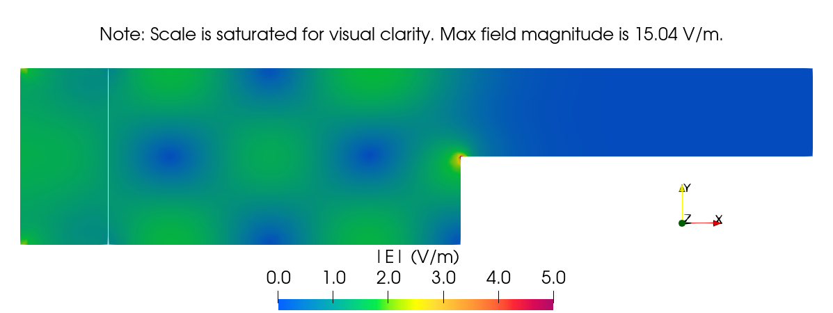
Figure 6: Field results of the evanescent wave decay benchmark study at 20GHz, using a rounded corner instead of a sharp one.

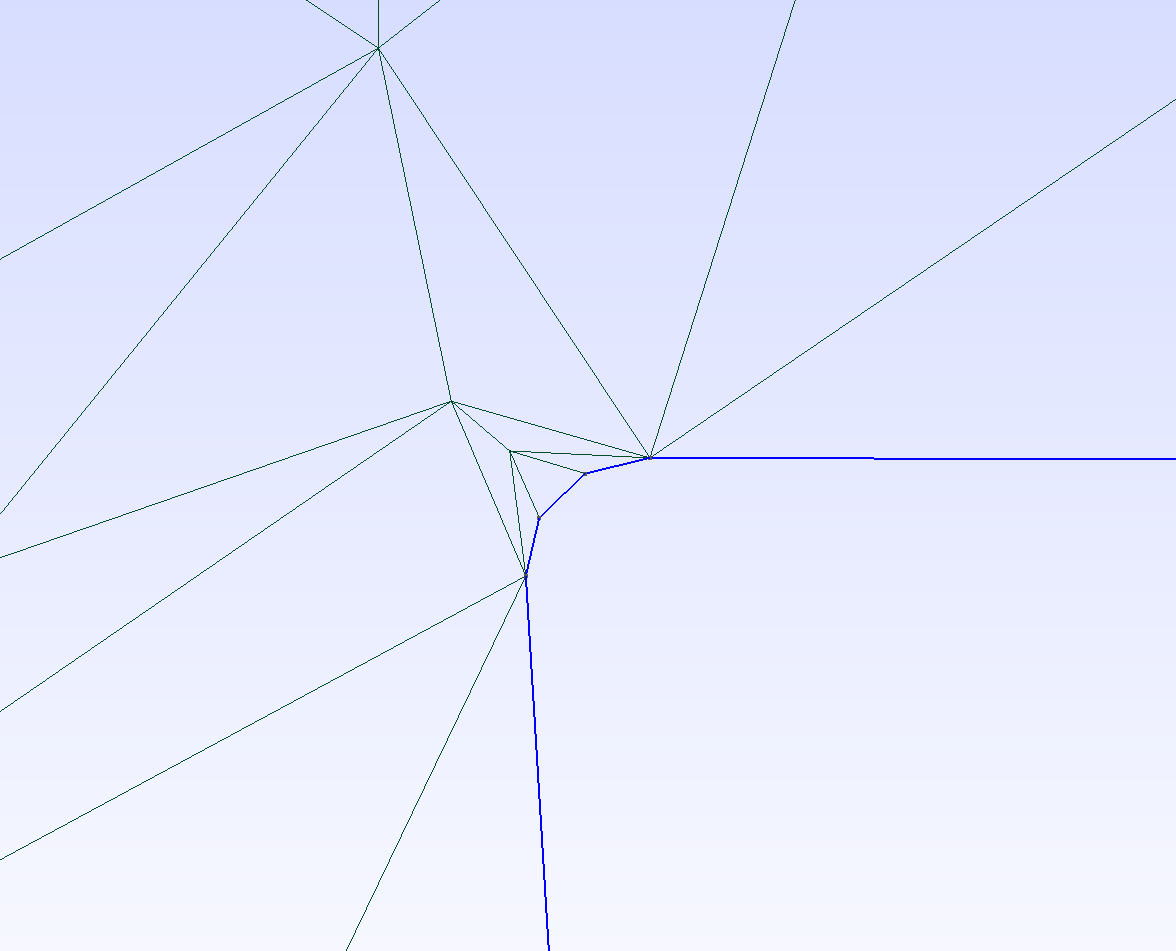
Figure 7: Rounded corner in waveguide geometry.

References

David J. Griffiths. Introduction to Electrodynamics. Prentice Hall, Upper Saddle River, New Jersey, USA, 3rd edition, 1999.

@book{griffiths-intro,
    author = "Griffiths, David J.",
    title = "Introduction to Electrodynamics",
    edition = "3rd",
    year = "1999",
    publisher = "Prentice Hall",
    address = "Upper Saddle River, New Jersey, USA"
}

Jian-Ming Jin. The Finite Element Method in Electromagnetics. John Wiley & Sons, Hoboken, New Jersey, USA, 3rd edition, 2014.

@book{jin-fem,
    author = "Jin, Jian-Ming",
    title = "The Finite Element Method in Electromagnetics",
    edition = "3rd",
    year = "2014",
    publisher = "John Wiley \\& Sons",
    address = "Hoboken, New Jersey, USA"
}

(modules/electromagnetics/test/tests/benchmarks/evanescent_wave/waveguide_discontinuous.geo)

// Discontinuous waveguide mesh for evanescent wave decay benchmark
// Waveguide length = 4.5 cm
// Waveguide width (entry) = 1 cm
// Waveguide width (exit) = 0.5 cm
// Discontinuity location = 2.5 cm
// Entry source width = 0.5 cm
// Entry source height = 1 cm
// Entry location (lower left coordinate) = (0.0, 0.0)

// Use global scaling factor of 0.004 in order to reproduce benchmark mesh in
// documentation, and use a factor of 0.01 to reproduce the test mesh


// Define corners and important points in the domain (with scaling factors)
Point(1) = {-0, 0, 0, 1.0};
Point(2) = {0.005, 0, 0, 1.0};
Point(3) = {0.025, 0, 0, 1.0};
Point(4) = {0, 0.010, 0, 1.0};
Point(5) = {0.005, 0.010, 0, 1.0};
Point(6) = {0.045, 0.010, 0, 1.0};
Point(7) = {0.045, 0.005, 0, 1.0};
Point(8) = {0.025, 0.005, 0, 0.0025};

// Connect the outer points
Line(1) = {1, 4};
Line(2) = {4, 5};
Line(3) = {5, 6};
Line(4) = {6, 7};
Line(5) = {7, 8};
Line(6) = {8, 3};
Line(7) = {3, 2};
Line(8) = {2, 1};

// Connect the dividing line between the source region and general vacuum region
Line(9) = {2, 5};

// Define loop for source region
Line Loop(1) = {1, 2, -9, 8};
Plane Surface(1) = {1};

// Define loop for general vacuum region
Line Loop(2) = {3, 4, 5, 6, 7, 9};
Plane Surface(2) = {2};

// Setup physical domains with labels
Physical Surface("source") = {1};
Physical Surface("vacuum") = {2};

// Setup sidesets
Physical Line("walls") = {3, 2, 8, 7, 6, 5};
Physical Line("port") = {1};
Physical Line("exit") = {4};

(modules/electromagnetics/test/tests/benchmarks/evanescent_wave/evanescent_wave.i)

# Evanescent wave decay benchmark
# frequency = 20 GHz
# eps_R = 1.0
# mu_R = 1.0

[Mesh]
  [fmg]
    type = FileMeshGenerator
    file = waveguide_discontinuous.msh
  []
[]

[Functions]
  [waveNumberSquared]
    type = ParsedFunction
    expression = '(2*pi*20e9/3e8)^2'
  []
  [omegaMu]
    type = ParsedFunction
    expression = '2*pi*20e9*4*pi*1e-7'
  []
  [beta]
    type = ParsedFunction
    expression = '2*pi*20e9/3e8'
  []
  [curr_real]
    type = ParsedVectorFunction
    expression_y = 1.0
  []
  [curr_imag] # defaults to '0.0 0.0 0.0'
    type = ParsedVectorFunction
  []
[]

[Variables]
  [E_real]
    family = NEDELEC_ONE
    order = FIRST
  []
  [E_imag]
    family = NEDELEC_ONE
    order = FIRST
  []
[]

[Kernels]
  [curlCurl_real]
    type = CurlCurlField
    variable = E_real
  []
  [coeff_real]
    type = VectorFunctionReaction
    variable = E_real
    function = waveNumberSquared
    sign = negative
  []
  [source_real]
    type = VectorCurrentSource
    variable = E_real
    component = real
    source_real = curr_real
    source_imag = curr_imag
    function_coefficient = omegaMu
    block = source
  []
  [curlCurl_imag]
    type = CurlCurlField
    variable = E_imag
  []
  [coeff_imag]
    type = VectorFunctionReaction
    variable = E_imag
    function = waveNumberSquared
    sign = negative
  []
  [source_imaginary]
    type = VectorCurrentSource
    variable = E_imag
    component = imaginary
    source_real = curr_real
    source_imag = curr_imag
    function_coefficient = omegaMu
    block = source
  []
[]

[BCs]
  [absorbing_left_real]
    type = VectorEMRobinBC
    variable = E_real
    component = real
    beta = beta
    coupled_field = E_imag
    mode = absorbing
    boundary = 'port'
  []
  [absorbing_right_real]
    type = VectorEMRobinBC
    variable = E_real
    component = real
    beta = beta
    coupled_field = E_imag
    mode = absorbing
    boundary = 'exit'
  []
  [absorbing_left_imag]
    type = VectorEMRobinBC
    variable = E_imag
    component = imaginary
    beta = beta
    coupled_field = E_real
    mode = absorbing
    boundary = 'port'
  []
  [absorbing_right_imag]
    type = VectorEMRobinBC
    variable = E_imag
    component = imaginary
    beta = beta
    coupled_field = E_real
    mode = absorbing
    boundary = 'exit'
  []
[]

[Preconditioning]
  [SMP]
    type = SMP
    full = true
  []
[]

[Executioner]
  type = Steady
  solve_type = 'NEWTON'
  petsc_options_iname = '-pc_type'
  petsc_options_value = 'lu'
[]

[Outputs]
  exodus = true
  print_linear_residuals = true
[]

[Debug]
  show_var_residual_norms = true
[]

Model Geometry
Governing Equations and Boundary Conditions
Model Parameters
Mesh
Evanescent Wave Decay Theory
Input File
Solution and Discussion
References