Running MALAMUTE and Viewing Results
Utilize a built MALAMUTE executable to run the desired input file. The command prompt’s printed outputs hold some valuable information. If there is an error, an error message will be automatically printed in the command prompt. Do not worry about the volumetric number of outputs shown under the “Pre-SMO residual” section, as this is normal for an input file. A way to observe how long the input file ran is to look at the Performance Graph at the end of the output in the command prompt. The first row in the graph will have the run time in seconds under Avg(s).
Performance information of running an input file with a die wall thickness of 5 mm and a time step of dt = 6 is shown below.
Performance Graph:
--------------------------------------------------------------------------------------------------------------------------------------------------------------------------
|                                Section                               | Calls |   Self(s)  |   Avg(s)   |    %   | Mem(MB) |  Total(s)  |   Avg(s)   |    %   | Mem(MB) |
--------------------------------------------------------------------------------------------------------------------------------------------------------------------------
| MalamuteTestApp (main)                                               |     1 |      0.007 |      0.007 |   0.00 |       2 |  12113.359 |  12113.359 | 100.00 |     249 |
|   Action::SetupMeshAction::Mesh::SetupMeshAction::act::setup_mesh    |     1 |      0.001 |      0.001 |   0.00 |       0 |      0.001 |      0.001 |   0.00 |       0 |
|   Action::SetupMeshAction::Mesh::SetupMeshAction::act::set_mesh_base |     2 |      0.012 |      0.006 |   0.00 |       3 |      0.012 |      0.006 |   0.00 |       3 |
|   MeshGeneratorSystem::createMeshGeneratorOrder                      |     1 |      0.000 |      0.000 |   0.00 |       0 |      0.000 |      0.000 |   0.00 |       0 |
|   ReferenceResidualProblem::computeUserObjects                       |     2 |      0.000 |      0.000 |   0.00 |       0 |      0.000 |      0.000 |   0.00 |       0 |
|   ReferenceResidualProblem::computeUserObjects                       |     3 |      0.000 |      0.000 |   0.00 |       0 |      0.000 |      0.000 |   0.00 |       0 |
|   ReferenceResidualProblem::outputStep                               |   353 |      0.049 |      0.000 |   0.00 |       0 |     83.045 |      0.235 |   0.69 |  -10896 |
|   Transient::PicardSolve                                             |   455 |      0.417 |      0.001 |   0.00 |       0 |  12027.898 |     26.435 |  99.29 |   11056 |
|     ReferenceResidualProblem::computeUserObjects                     |  3228 |      0.103 |      0.000 |   0.00 |       0 |      0.103 |      0.000 |   0.00 |       0 |
|     ReferenceResidualProblem::outputStep                             |  1365 |      0.107 |      0.000 |   0.00 |       0 |      0.110 |      0.000 |   0.00 |       0 |
|     ReferenceResidualProblem::solve                                  |   455 |   3876.046 |      8.519 |  32.00 |   11291 |  11949.174 |     26.262 |  98.64 |   11072 |
|       ReferenceResidualProblem::computeResidualInternal              |   455 |      0.008 |      0.000 |   0.00 |       0 |    176.756 |      0.388 |   1.46 |     -15 |
|         ReferenceResidualProblem::computeUserObjects                 |   910 |      0.004 |      0.000 |   0.00 |       0 |      0.004 |      0.000 |   0.00 |       0 |
|       ReferenceResidualProblem::computeResidualInternal              |  5586 |      0.106 |      0.000 |   0.00 |       0 |   2006.776 |      0.359 |  16.57 |     -36 |
|         ReferenceResidualProblem::computeUserObjects                 | 11172 |      0.064 |      0.000 |   0.00 |       0 |      0.064 |      0.000 |   0.00 |       0 |
|       ReferenceResidualProblem::computeJacobianInternal              |  5131 |      0.083 |      0.000 |   0.00 |       0 |   5518.112 |      1.075 |  45.55 |    -128 |
|         ReferenceResidualProblem::computeUserObjects                 | 10262 |      0.050 |      0.000 |   0.00 |       0 |      0.050 |      0.000 |   0.00 |       0 |
|   Transient::final                                                   |     1 |      0.000 |      0.000 |   0.00 |       0 |      0.000 |      0.000 |   0.00 |       0 |
|     ReferenceResidualProblem::computeUserObjects                     |     2 |      0.000 |      0.000 |   0.00 |       0 |      0.000 |      0.000 |   0.00 |       0 |
|     ReferenceResidualProblem::outputStep                             |     1 |      0.000 |      0.000 |   0.00 |       0 |      0.000 |      0.000 |   0.00 |       0 |
--------------------------------------------------------------------------------------------------------------------------------------------------------------------------
Finished Executing                                                                       [12112.10 s] [  302 MB]
Viewing Results in ParaView
There are two “output” files generated after running an input file: a csv file and .e file. To open a .e file in ParaView, open ParaView, navigate to ‘File’ and select ‘Open’. You'll need to collect the file path of the .e file, which can be done by using the 'pwd' command in the Terminal. Once you have the file path, copy and paste it into the 'Name:' box and click OK.
The input file and csv & .e files will share the same file name, with .i or .e on the end of the file name being one difference, and the word “out” attached to the end of the .e and csv file being another difference.
We will now see the file name on the left side of the ParaView menu under “Pipeline Browser.” Click “apply” under the “Properties” section to allow for “Reflect” annotation later. Make sure to click the dotted ellipse next to the file name to ensure an eyeball icon appears, to ensure you can observe the DCS machine’s geometry. Also, be sure to select the Toggle Color Legend Visibility icon, which is the leftmost icon in Figure 1.

Figure 1: ParaView screenshot.
To view a complete 2D cross-section of the DCS-5 machine, navigate through 'Filters' to 'Alphabetical' and then select 'Reflect.'
Recommended procedure: To compare two different scenarios, such as potential change and temperature change across the DCS machine, use the Split Horizontal Axis icon then click ‘Render View.’ Now, click one of the two click ‘Render View’ sections and see that a blue border surrounds this box. Use the dropdown menu that shows “Solid Color” to select scenarios titled “potential, temperature, heat_transfer_radiation, and electric_field.”
When editing the color map, select the desired window and click the Edit Color Map icon, which is second from the left in the screenshot shown above. From there, click the 'Select a color map from default presets' dropdown box. For potential, the Viridis color map is recommended, and for temperature, use Inferno. When adjusting the data range, use the “scale for all timesteps” option to find the required minimum and maximum values.
Viewing Results in Excel
The second output type created by running the input file is called a csv file. To open a csv file in Excel, navigate to File Explorer or Finder and locate the desired csv file, then open the csv file with Excel.
Excel Usage Example
Use dt = 6 for the required timestep in the [Executioner] to allow for a quicker runtime compared to lower or higher timestep values, while also limiting percent error versus higher timesteps. While wall thickness varies, the max temperature and overall temperature of the powder will decrease as the wall thickness increases. This trend could be viewed by graphing Temperature Variation vs Die Wall Thickness for each of the five die wall thicknesses. The time at which the max temperature varied slightly between die wall thickness. The timeframe range for when the max temperature is reached, according to a study ran using MALAMUTE, is between 954 and 966 seconds.
The highest temperature out of all the wall thicknesses occurred with the 5mm die wall thickness at 954 seconds. For a visual representation of various aspects such as electric potential, temperature, heat transfer radiation, and electric field, we recommend viewing these aspects in a program such as ParaView in the timeframe range of 954 and 966 seconds. The approximate time values in which the max temperature occurs is shown in a chart here while discussing the sizable difference between each of the max temperature values for the various die wall thicknesses.
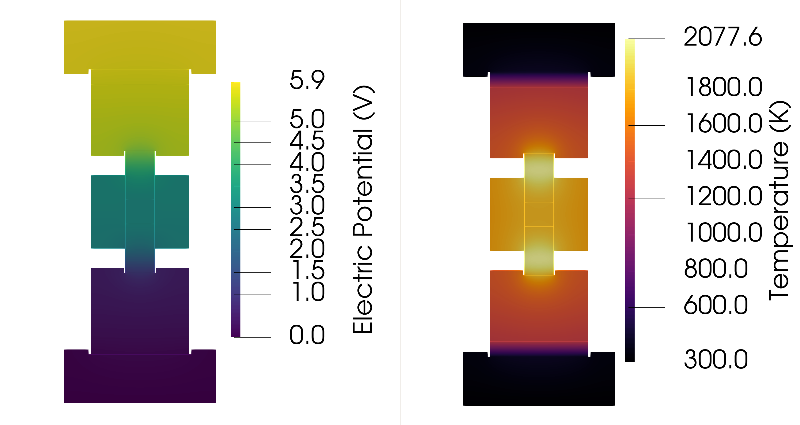
Figure 2: Electric Potential and Temperature Contour Plots in ParaView.