Concluding Remarks
This tutorial was created with the intention of providing initial instructions for MALAMUTE by exploring the relation between temperature and die wall thickness. After visualizing in Excel, the Temperature vs Time data for each wall thickness, we see that the overall temperature decreases as the wall thickness increases. One exception to this pattern is the similar temperature values approximately halfway through the linear portion (approximately t = 1240 s to t = 1260 s) of the “cooling process”. Also, as the die wall thickness increases, the time at which max temperature occurs is higher.
Figure 1: Temperature vs Time data for each of the five wall thicknesses
There is a sizable difference between each of the max temperature values for the various die wall thicknesses and a slight difference at the time which these max temperatures occur, as shown in Figure 2. This occurrence might be explained by the electric field contour plots shown in Figure 4.
Figure 2: Max Temperature vs Simulation Time.
Regarding the contour plots at max temperature formed by ParaView, we observed patterns regarding temperature and electric potential. The graphite die wall thickness increase leads to a cooler temperature of the powder and die wall as shown by the ‘temperature’ contour plot, in Figure 3 for example. The temperature difference due to die wall thickness is visualized in the figures below by a sharp color shade difference between the 5 mm and 25 mm die thickness contour plots shown below. Also, this color change and thus gradual temperature decrease is seen progressively across all five die wall thickness examples. Especially if viewing the contour plots starting from the 5 mm die wall thickness temperature contour plot, then ending with the 25 mm die wall thickness temperature contour plot. Also, the center of the graphite plungers is generally hotter than the die wall and the powder casing, with an almost white color having an approximate value of 2.3e+03 K.
The electric potential on the toolset steadily decreases from the top of the toolset to the bottom of it, as observed in the contour plot below. This indicates that the direction of electric current is from top to bottom, and this current direction corresponds with how the DCS-5 machine is constructed.
Figure 3: Electrical Potential and Temperature Contour Plots.
Electric field values slightly between different wall thickness, but noticeably changes on the graphite spacers. The electric field is highly concentrated in the center of these graphite spacers and seems to correspond with the higher temperature values in the same spot. This phenomenon is shown in Figure 5, for example. However, the powder casing and die wall do not experience a similar spike in temperature or electric potential to the graphite spacers and may need to be considered when analyzing an EFAS toolset.
Figure 4: Electric Field and Temperature Contour Plots for a 5 mm wall thickness at t = 954 seconds.
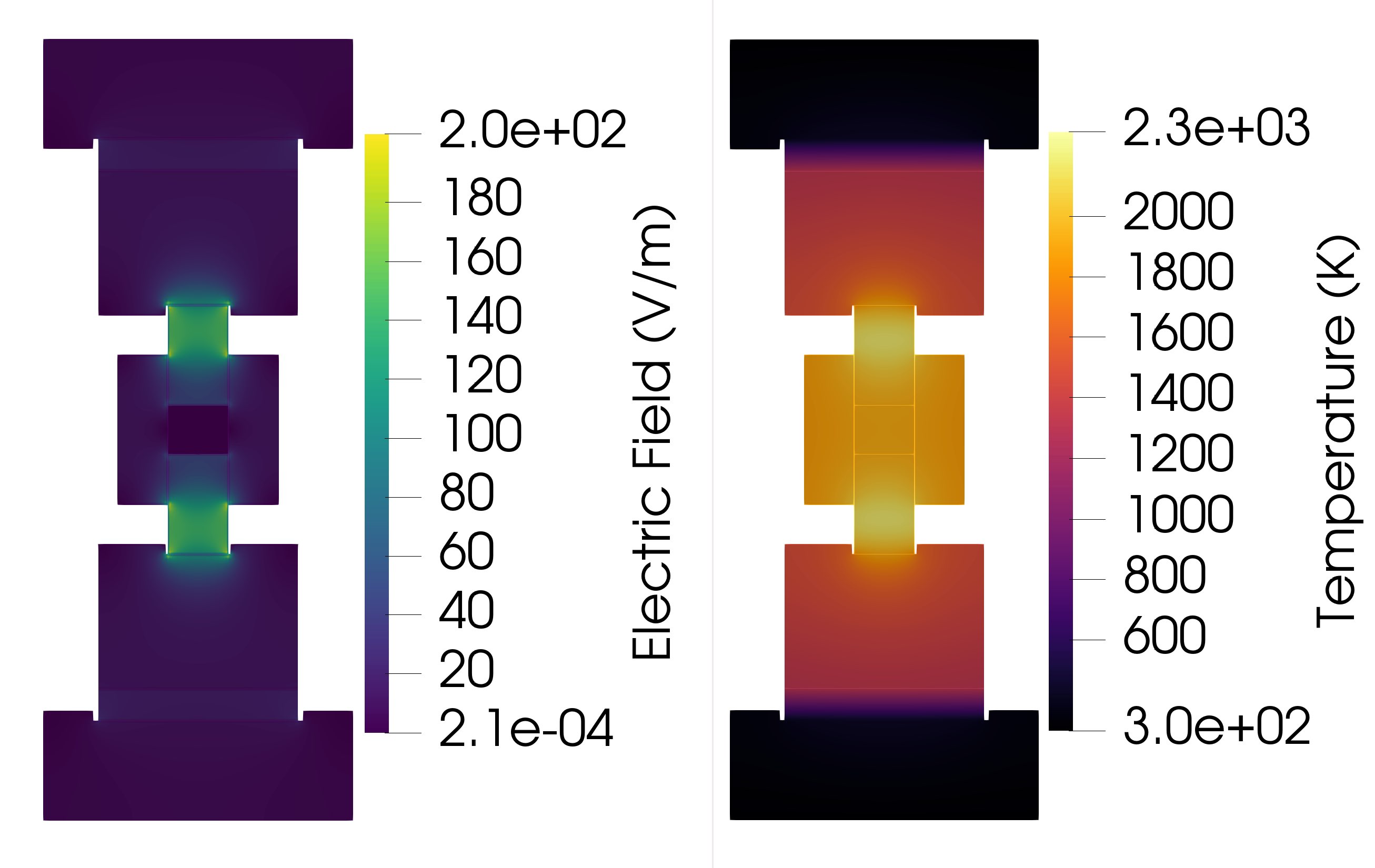
Figure 5: Electric Field and Temperature Contour Plots for a 10 mm wall thickness at t = 960 seconds.
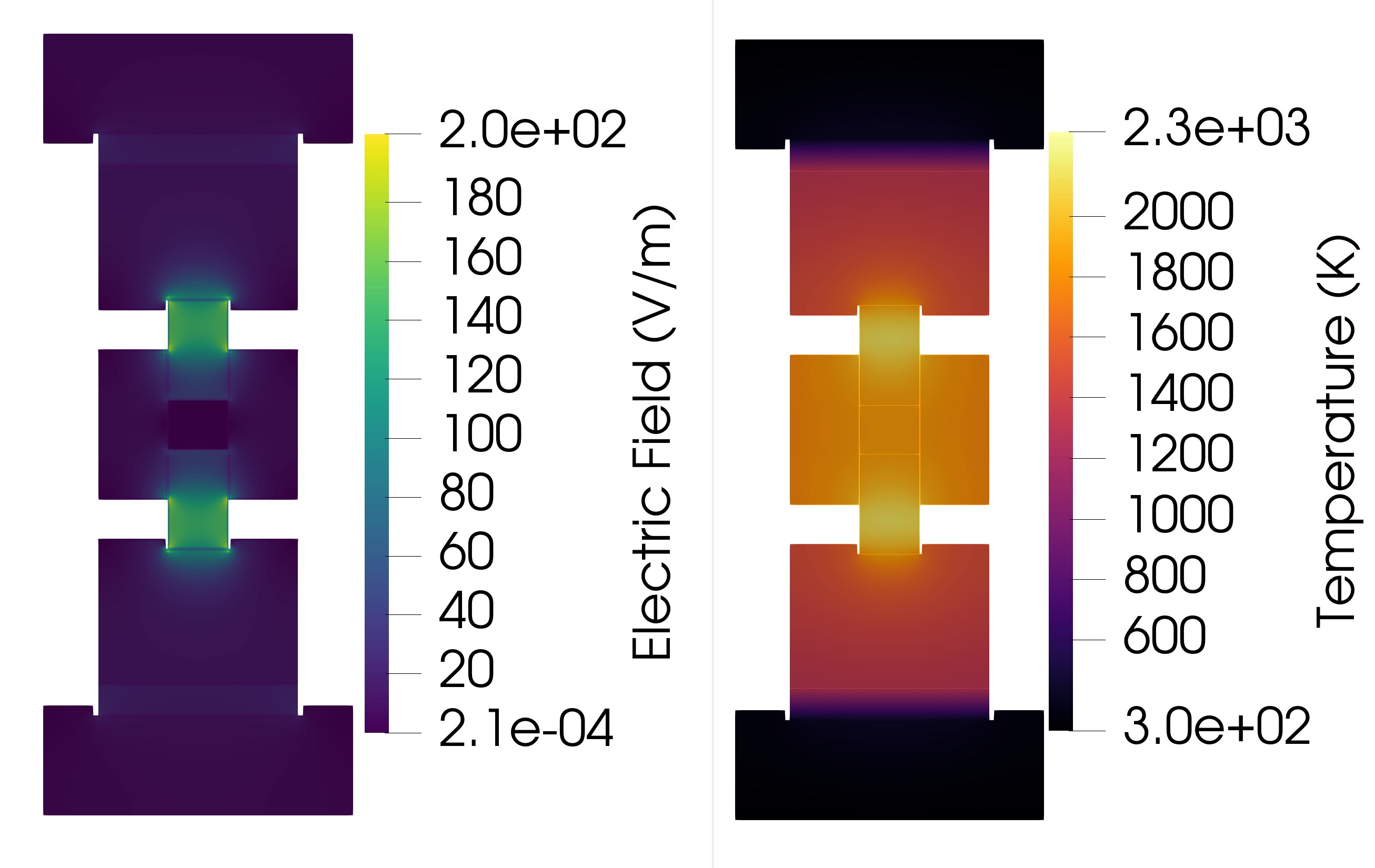
Figure 6: Electric Field and Temperature Contour Plots for a 13.875 mm wall thickness at t = 960 seconds.
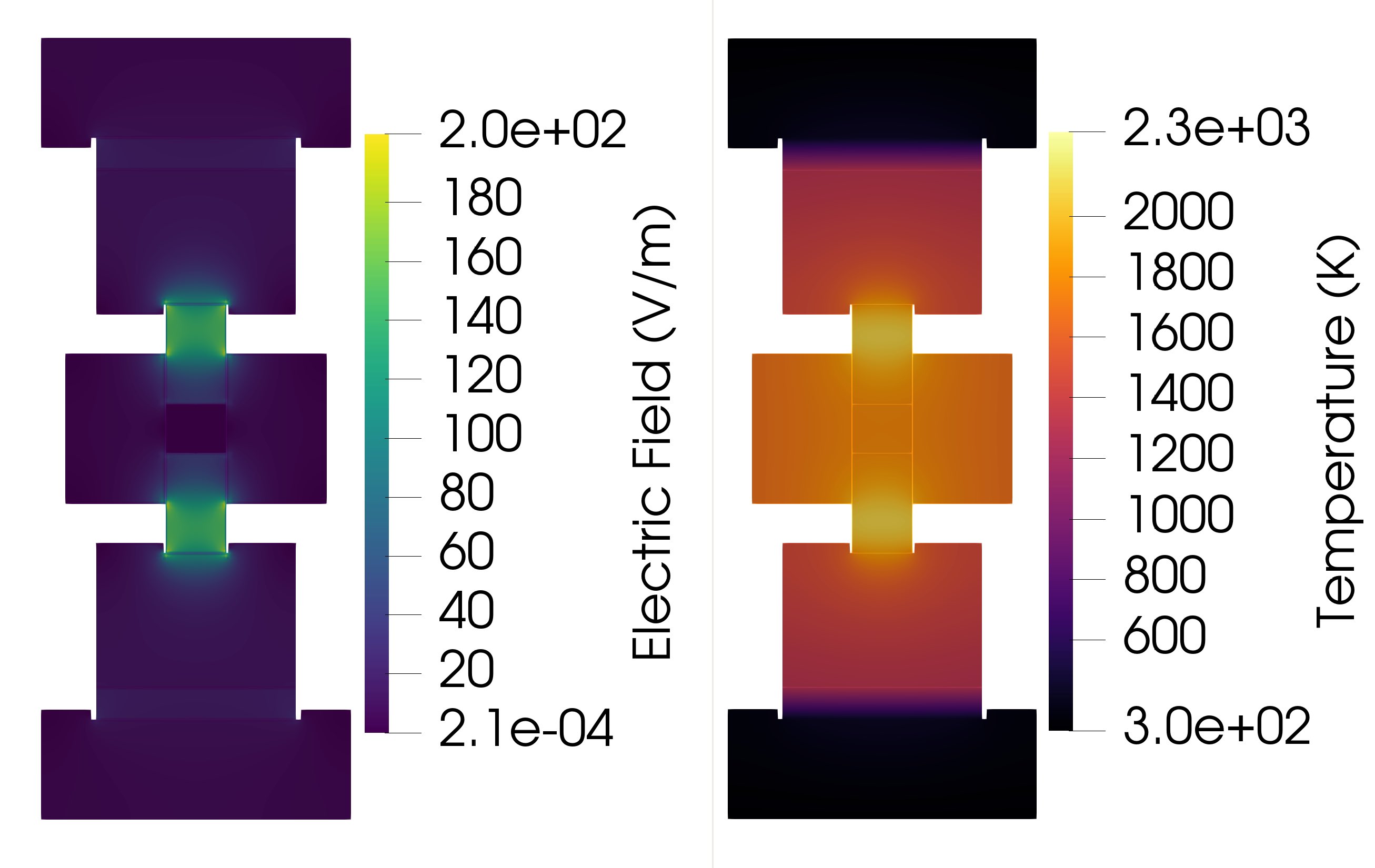
Figure 7: Electric Field and Temperature Contour Plots for a 20 mm wall thickness at t = 966 seconds.
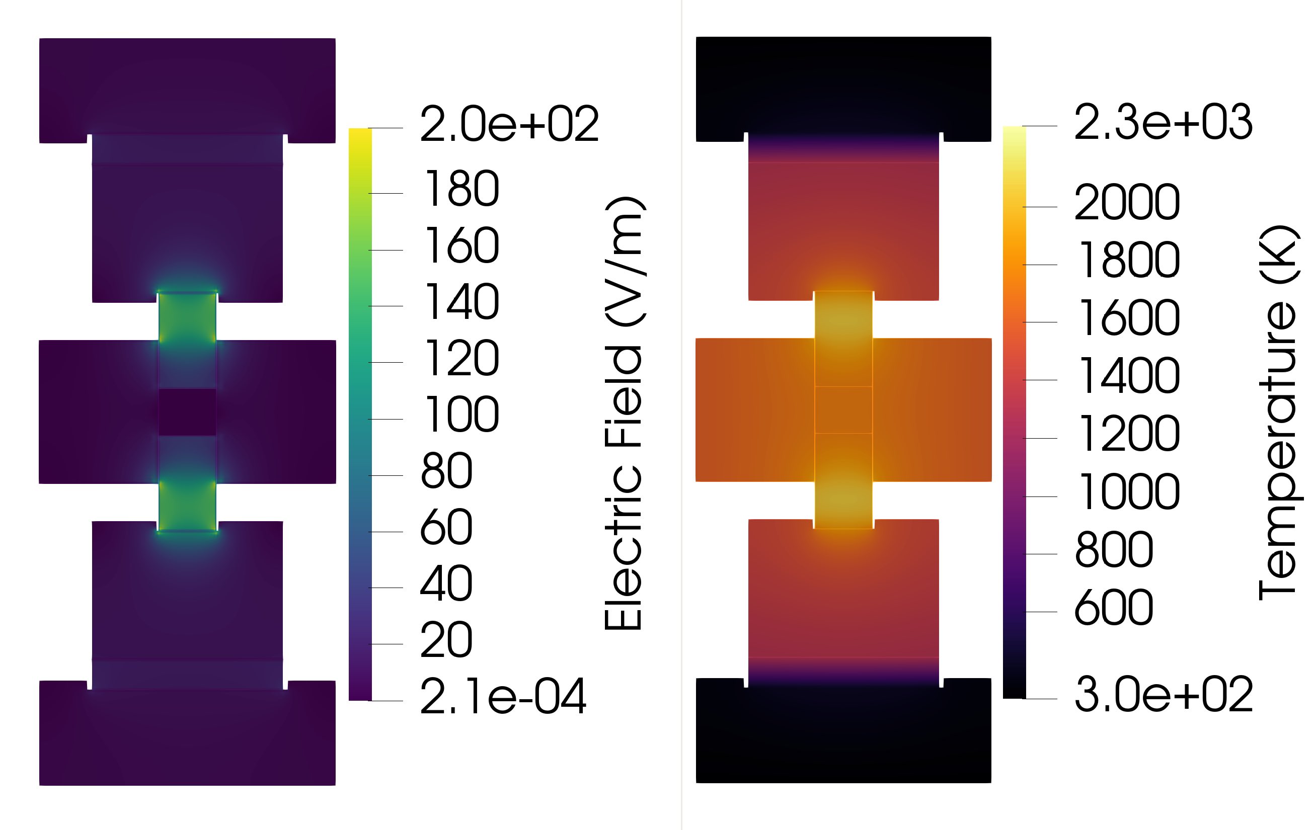
Figure 8: Electric Field and Temperature Contour Plots for a 25 mm wall thickness at t = 972 seconds.
Conclusion
As mentioned in the beginning of this tutorial, temperature distribution as a function of die geometry is crucial in the EFAS process. A thicker die wall thickness led to a lower temperature on the die wall, and thus a lower overall temperature on the powder casing. A die wall being too thin caused an ineffective management of temperature gradients, as shown in the journal article at the beginning of this tutorial. It is therefore essential to optimize the die wall thickness to ensure consistent heating and the integrity of the sintering process.
We successfully performed a basic one-factor study involving a parametric analysis, limiting the independent variable to five different die wall thicknesses (e.g., 5 mm, 10 mm, 13.875 mm, 20 mm, 25 mm).
The primary objective of this tutorial was to observe how the temperature distribution within the DCS-5 tooling stack varies with die wall thickness.
We achieved this goal by utilizing temperature and electrical potential contour fields as well as time versus history graphs to identify any patterns of temperature localization that emerged. Analysis of these results was completed effectively to determine the impact of the die wall thickness relative to temperature as predicted by these MALAMUTE simulations.