RTES Stochastic Simulation: Parametric Sweeping

Problem Statement

The performance of RTES is highly relevant to the formation characteristics of the site and operational conditions, which are the critical attributes of the techno-economic performance of a potential site. This example demonstrates the capability of FALCON to generate synthetic data for RTES potential site identification using automated stochastic simulation. Following Jin et al. (2022) and Jin et al. (2021), a generic caprock-reservoir-bedrock formation with varying formation characteristics (permeability, porosity, thermal conductivity, thickness, in-situ temperature and pore pressure) was simulated. Figure 1 shows the boundary conditions and the geometry of the generic formation. Note a common doublet well configuration was adopted for this case, and half of the domain was simulated due to symmetry. In addition to the formation characteristics, the operational conditions of injection rate, fluid injection temperature, and well distance were also investigated to reveal their influence on RTES performance.

Figure 1: Geometry and boundary conditions of the generic formation with doublet system for simulation.

FALCON input files

Physics simulation input file

In this example, only the physics of heat transfer and fluid flow is considered, and the formation is assumed homogeneous and fully saturated with uniform in-situ temperature and pore pressure. To enable the flexbility of convergence implemented in unsaturated kernels, we used the PorousFlowUnsaturated Action as


[PorousFlowUnsaturated]
  relative_permeability_type = COREY
  relative_permeability_exponent = 0
  add_darcy_aux = true
  coupling_type = ThermoHydro
  gravity = '0 0 -9.8'
  porepressure = porepressure
  temperature = temperature
  fp = tabulated_water
  use_displaced_mesh = false
[]

Mesh: The generic formation was meshed using CUBIT. As a result, the thickness of formation was descretized into 10 cases with thickness ranging from 10 meters to 100 meters. The loading of the Exodus mesh file in input file is via


[Mesh]
  [./fmg]
    type = FileMeshGenerator
    file = base_final_50.e
  []
[]

Initial Condition: Given the initial temperature and pore pressure is correlated with depth in general as

$(1)var element = document.getElementById("moose-equation-95c87aaa-1ef4-4d80-9499-dd51acfb245b");katex.render("P_0(Z)= \\begin{cases} \\rho_f gZ, \\quad Z<2000 \\\\ \\rho_f gZ + (Z-2000)\\rho_f g, \\quad Z\\geq 2000 \\end{cases} ", element, {displayMode:true,throwOnError:false});$ $(2)var element = document.getElementById("moose-equation-73742184-60b9-4fb2-b690-29e2f5392ad3");katex.render("T_0(Z) = 26.67 + 0.02005Z ", element, {displayMode:true,throwOnError:false});$

We coded the equation in the input file as


depth =  2000 
pp_ini_bc = ${fparse if(depth<=2000, 1000*9.8*depth, 1000*9.8*depth+(depth-2000)*9.8*1000)}
T_ini_bc  = ${fparse (80+3.28084*depth*1.1/100-32)*5/9 + 273.15}

and we assigned the initial condition as

[ICs<<<{"href": "../syntax/ICs/index.html"}>>>]
  [./init_pp]
    type = FunctionIC<<<{"description": "An initial condition that uses a normal function of x, y, z to produce values (and optionally gradients) for a field variable.", "href": "../source/ics/FunctionIC.html"}>>>
    function<<<{"description": "The initial condition function."}>>> = ${pp_ini_bc}
    variable<<<{"description": "The variable this initial condition is supposed to provide values for."}>>> = porepressure
  [../]
  [./init_temp]
    type = ConstantIC<<<{"description": "Sets a constant field value.", "href": "../source/ics/ConstantIC.html"}>>>
    value<<<{"description": "The value to be set in IC"}>>> = ${T_ini_bc}
    variable<<<{"description": "The variable this initial condition is supposed to provide values for."}>>> = temperature
  [../]
[]

Boundary Condition: The simulated domain has a 1 km length in the horizontal direction, and we assigned drained boundary conditions with pore pressure and temperature equal to the initial values for all side faces, except the symmetrical surface. While the top and bottom surfaces were undrained. The input file section is !listing examples/rtes_stochastic/base_cycle_50.i block=BCs

Operation: In order to perform parametric study of operational conditions, we first defined variables in input file as


distance_between_wells = 200
pro_well_x = ${fparse 0.1 + distance_between_wells / 2}
inj_well_x  = ${fparse 0.1 - distance_between_wells / 2}
well_length = 50  #fixed number in accordance with the mesh
aquifer_mid= ${fparse 0 + 0}
aquifer_top= ${fparse 0 + well_length/2}
aquifer_bot= ${fparse 0 - well_length/2}
#---Define a scalar variable to sweep 
inj_ext_exponent = 1.5
inj_ext_flux= ${fparse 10^inj_ext_exponent / well_length / 2 }
injection_temp = 473.15

The above variables help to assign injection parameters for the operation. A typical seasonal operation with injection-storage-extraction-rest cycle was simulated. In the summer, cold fluid is extracted from the cold well and heated to an assigned temperature, then re-injected into the reservoir through the hot well at the same rate as the extraction. The same injection and extraction rates at the charging summer period ensure the pore pressure disturbance in the reservoir is minimized. In the winter, fluid is extracted from the hot well for the generation of electricity with the post-generation energy-depleted fluid being injected back into the reservoir through the cold well. The extraction and injection rates during the winter discharging period also remain the same as the summer charging time, and the injected fluid temperature into the cold well is the same as the initial reservoir temperature. For the fall and spring seasons, no fluid circulation is performed. Note in this example, high-temperature RTES is targeted to generate electricity when thermal energy is extracted. The energy extraction period is terminated when the temperature of the extracted hot well fluid is reduced by 20\% in relation to the difference between the fluid injection temperature and the initial reservoir temperature, i.e., we stop discharging when the temperature of the hot well $var element = document.getElementById("moose-equation-75e88521-408c-495e-90f4-5e66ac2eb93e");katex.render("T_{hot}", element, {displayMode:false,throwOnError:false});$ satisfies $var element = document.getElementById("moose-equation-16ec8ee8-2a32-4a15-9da0-37ba9c5f9368");katex.render("(T_{hot}-T_0)/(T_i-T_0)<80\\%", element, {displayMode:false,throwOnError:false});$ . This high cut-off temperature is adopted to ensure the extracted hot fluid can be used for electricity generation. This operation was achieved by the combination of DiracKernels, Controls, Functions, and Postprocessors of FALCON.

First, we defined three groups of DiracKernels to realize the charging, discharging and rest operations from the two wells. Note the predefined variables of injection/extraction rate, well locations, and injection temperature are used as

[DiracKernels<<<{"href": "../syntax/DiracKernels/index.html"}>>>]
  [./charge_injection_P]
    type = PorousFlowPolyLineSink<<<{"description": "Approximates a polyline sink by using a number of point sinks with given weighting whose positions are read from a file.  NOTE: if you are using PorousFlowPorosity that depends on volumetric strain, you should set strain_at_nearest_qp=true in your GlobalParams, to ensure the nodal Porosity Material uses the volumetric strain at the Dirac quadpoints, and can therefore be computed", "href": "../source/dirackernels/PorousFlowPolyLineSink.html"}>>>
    fluid_phase<<<{"description": "The fluid phase whose pressure (and potentially mobility, enthalpy, etc) controls the flux to the line sink.  For p_or_t=temperature, and without any use_*, this parameter is irrelevant"}>>> = 0
    variable<<<{"description": "The name of the variable that this residual object operates on"}>>> = porepressure
    SumQuantityUO<<<{"description": "User Object of type=PorousFlowSumQuantity in which to place the total outflow from the line sink for each time step."}>>> = fluid_mass_in_inc
    line_base<<<{"description": "Line base point x,y,z coordinates.  This is the same format as a single-line point_file. Note this is only used if there is no point file specified."}>>> = '1 ${inj_well_x} 0 ${aquifer_bot}'
    line_length<<<{"description": "Line length.  Note this is only used if there is only one point in the point_file."}>>> = ${well_length}
    line_direction<<<{"description": "Line direction.  Note this is only used if there is only one point in the point_file."}>>> = '0 0 1'
    p_or_t_vals<<<{"description": "Tuple of pressure (or temperature) values.  Must be monotonically increasing."}>>> = '-1e9 1e9'
    fluxes<<<{"description": "Tuple of flux values (measured in kg.m^-1.s^-1 if no 'use_*' are employed).  These flux values are multiplied by the line-segment length to achieve a flux in kg.s^-1.  A piecewise-linear fit is performed to the (p_or_t_vals,flux) pairs to obtain the flux at any arbitrary pressure (or temperature).  If a quad-point pressure is less than the first pressure value, the first flux value is used.  If quad-point pressure exceeds the final pressure value, the final flux value is used.  This flux is OUT of the medium: hence positive values of flux means this will be a SINK, while negative values indicate this flux will be a SOURCE."}>>> = '-${inj_ext_flux} -${inj_ext_flux}' # ~5 kg/s over length of 10(injection_length)/2
  [../]
  [./charge_injection_T]
    type = EnthalpySink
    fluid_phase = 0
    variable = temperature
    SumQuantityUO = heat_enthalpy_in_inc
    line_base = '1 ${inj_well_x} 0 ${aquifer_bot}'
    line_length = ${well_length}
    line_direction = '0 0 1'
    pressure = porepressure
    T_in = ${injection_temp}
    fp = tabulated_water
    p_or_t_vals = '-1e9 1e9'
    fluxes = '-${inj_ext_flux} -${inj_ext_flux}'
  [../]
  [./charge_production_P]
    type = PorousFlowPolyLineSink<<<{"description": "Approximates a polyline sink by using a number of point sinks with given weighting whose positions are read from a file.  NOTE: if you are using PorousFlowPorosity that depends on volumetric strain, you should set strain_at_nearest_qp=true in your GlobalParams, to ensure the nodal Porosity Material uses the volumetric strain at the Dirac quadpoints, and can therefore be computed", "href": "../source/dirackernels/PorousFlowPolyLineSink.html"}>>>
    fluid_phase<<<{"description": "The fluid phase whose pressure (and potentially mobility, enthalpy, etc) controls the flux to the line sink.  For p_or_t=temperature, and without any use_*, this parameter is irrelevant"}>>> = 0
    variable<<<{"description": "The name of the variable that this residual object operates on"}>>> = porepressure
    SumQuantityUO<<<{"description": "User Object of type=PorousFlowSumQuantity in which to place the total outflow from the line sink for each time step."}>>> = fluid_mass_out_inc
    line_base<<<{"description": "Line base point x,y,z coordinates.  This is the same format as a single-line point_file. Note this is only used if there is no point file specified."}>>> = '1 ${pro_well_x} 0 ${aquifer_bot}'
    line_length<<<{"description": "Line length.  Note this is only used if there is only one point in the point_file."}>>> = ${well_length}
    line_direction<<<{"description": "Line direction.  Note this is only used if there is only one point in the point_file."}>>> = '0 0 1'
    p_or_t_vals<<<{"description": "Tuple of pressure (or temperature) values.  Must be monotonically increasing."}>>> = '-1e9 1e9'
    fluxes<<<{"description": "Tuple of flux values (measured in kg.m^-1.s^-1 if no 'use_*' are employed).  These flux values are multiplied by the line-segment length to achieve a flux in kg.s^-1.  A piecewise-linear fit is performed to the (p_or_t_vals,flux) pairs to obtain the flux at any arbitrary pressure (or temperature).  If a quad-point pressure is less than the first pressure value, the first flux value is used.  If quad-point pressure exceeds the final pressure value, the final flux value is used.  This flux is OUT of the medium: hence positive values of flux means this will be a SINK, while negative values indicate this flux will be a SOURCE."}>>> = '${inj_ext_flux} ${inj_ext_flux}'
  [../]
  [./charge_production_T]
    type = PorousFlowPolyLineSink<<<{"description": "Approximates a polyline sink by using a number of point sinks with given weighting whose positions are read from a file.  NOTE: if you are using PorousFlowPorosity that depends on volumetric strain, you should set strain_at_nearest_qp=true in your GlobalParams, to ensure the nodal Porosity Material uses the volumetric strain at the Dirac quadpoints, and can therefore be computed", "href": "../source/dirackernels/PorousFlowPolyLineSink.html"}>>>
    fluid_phase<<<{"description": "The fluid phase whose pressure (and potentially mobility, enthalpy, etc) controls the flux to the line sink.  For p_or_t=temperature, and without any use_*, this parameter is irrelevant"}>>> = 0
    variable<<<{"description": "The name of the variable that this residual object operates on"}>>> = temperature
    SumQuantityUO<<<{"description": "User Object of type=PorousFlowSumQuantity in which to place the total outflow from the line sink for each time step."}>>> = heat_enthalpy_out_inc
    line_base<<<{"description": "Line base point x,y,z coordinates.  This is the same format as a single-line point_file. Note this is only used if there is no point file specified."}>>> = '1 ${pro_well_x} 0 ${aquifer_bot}'
    line_length<<<{"description": "Line length.  Note this is only used if there is only one point in the point_file."}>>> = ${well_length}
    line_direction<<<{"description": "Line direction.  Note this is only used if there is only one point in the point_file."}>>> = '0 0 1'
    use_enthalpy<<<{"description": "Multiply the flux by the fluid enthalpy"}>>> = true
    p_or_t_vals<<<{"description": "Tuple of pressure (or temperature) values.  Must be monotonically increasing."}>>> = '-1e9 1e9'
    fluxes<<<{"description": "Tuple of flux values (measured in kg.m^-1.s^-1 if no 'use_*' are employed).  These flux values are multiplied by the line-segment length to achieve a flux in kg.s^-1.  A piecewise-linear fit is performed to the (p_or_t_vals,flux) pairs to obtain the flux at any arbitrary pressure (or temperature).  If a quad-point pressure is less than the first pressure value, the first flux value is used.  If quad-point pressure exceeds the final pressure value, the final flux value is used.  This flux is OUT of the medium: hence positive values of flux means this will be a SINK, while negative values indicate this flux will be a SOURCE."}>>> = '${inj_ext_flux} ${inj_ext_flux}'
  [../]

  [./recover_production_P]
    type = PorousFlowPolyLineSink<<<{"description": "Approximates a polyline sink by using a number of point sinks with given weighting whose positions are read from a file.  NOTE: if you are using PorousFlowPorosity that depends on volumetric strain, you should set strain_at_nearest_qp=true in your GlobalParams, to ensure the nodal Porosity Material uses the volumetric strain at the Dirac quadpoints, and can therefore be computed", "href": "../source/dirackernels/PorousFlowPolyLineSink.html"}>>>
    fluid_phase<<<{"description": "The fluid phase whose pressure (and potentially mobility, enthalpy, etc) controls the flux to the line sink.  For p_or_t=temperature, and without any use_*, this parameter is irrelevant"}>>> = 0
    variable<<<{"description": "The name of the variable that this residual object operates on"}>>> = porepressure
    SumQuantityUO<<<{"description": "User Object of type=PorousFlowSumQuantity in which to place the total outflow from the line sink for each time step."}>>> = fluid_mass_in_inc
    line_base<<<{"description": "Line base point x,y,z coordinates.  This is the same format as a single-line point_file. Note this is only used if there is no point file specified."}>>> = '1 ${inj_well_x} 0 ${aquifer_bot}'
    line_length<<<{"description": "Line length.  Note this is only used if there is only one point in the point_file."}>>> = ${well_length}
    line_direction<<<{"description": "Line direction.  Note this is only used if there is only one point in the point_file."}>>> = '0 0 1'
    p_or_t_vals<<<{"description": "Tuple of pressure (or temperature) values.  Must be monotonically increasing."}>>> = '-1e9 1e9'
    fluxes<<<{"description": "Tuple of flux values (measured in kg.m^-1.s^-1 if no 'use_*' are employed).  These flux values are multiplied by the line-segment length to achieve a flux in kg.s^-1.  A piecewise-linear fit is performed to the (p_or_t_vals,flux) pairs to obtain the flux at any arbitrary pressure (or temperature).  If a quad-point pressure is less than the first pressure value, the first flux value is used.  If quad-point pressure exceeds the final pressure value, the final flux value is used.  This flux is OUT of the medium: hence positive values of flux means this will be a SINK, while negative values indicate this flux will be a SOURCE."}>>> = '${inj_ext_flux} ${inj_ext_flux}' # ~5 kg/s over length of 10(injection_length)/2
  [../]
  [./recover_production_T]
    type = PorousFlowPolyLineSink<<<{"description": "Approximates a polyline sink by using a number of point sinks with given weighting whose positions are read from a file.  NOTE: if you are using PorousFlowPorosity that depends on volumetric strain, you should set strain_at_nearest_qp=true in your GlobalParams, to ensure the nodal Porosity Material uses the volumetric strain at the Dirac quadpoints, and can therefore be computed", "href": "../source/dirackernels/PorousFlowPolyLineSink.html"}>>>
    fluid_phase<<<{"description": "The fluid phase whose pressure (and potentially mobility, enthalpy, etc) controls the flux to the line sink.  For p_or_t=temperature, and without any use_*, this parameter is irrelevant"}>>> = 0
    variable<<<{"description": "The name of the variable that this residual object operates on"}>>> = temperature
    SumQuantityUO<<<{"description": "User Object of type=PorousFlowSumQuantity in which to place the total outflow from the line sink for each time step."}>>> = heat_enthalpy_in_inc
    line_base<<<{"description": "Line base point x,y,z coordinates.  This is the same format as a single-line point_file. Note this is only used if there is no point file specified."}>>> = '1 ${inj_well_x} 0 ${aquifer_bot}'
    line_length<<<{"description": "Line length.  Note this is only used if there is only one point in the point_file."}>>> = ${well_length}
    line_direction<<<{"description": "Line direction.  Note this is only used if there is only one point in the point_file."}>>> = '0 0 1'
    use_enthalpy<<<{"description": "Multiply the flux by the fluid enthalpy"}>>> = true
    p_or_t_vals<<<{"description": "Tuple of pressure (or temperature) values.  Must be monotonically increasing."}>>> = '-1e9 1e9'
    fluxes<<<{"description": "Tuple of flux values (measured in kg.m^-1.s^-1 if no 'use_*' are employed).  These flux values are multiplied by the line-segment length to achieve a flux in kg.s^-1.  A piecewise-linear fit is performed to the (p_or_t_vals,flux) pairs to obtain the flux at any arbitrary pressure (or temperature).  If a quad-point pressure is less than the first pressure value, the first flux value is used.  If quad-point pressure exceeds the final pressure value, the final flux value is used.  This flux is OUT of the medium: hence positive values of flux means this will be a SINK, while negative values indicate this flux will be a SOURCE."}>>> = '${inj_ext_flux} ${inj_ext_flux}'
  [../]
  [./recover_injection_P]
    type = PorousFlowPolyLineSink<<<{"description": "Approximates a polyline sink by using a number of point sinks with given weighting whose positions are read from a file.  NOTE: if you are using PorousFlowPorosity that depends on volumetric strain, you should set strain_at_nearest_qp=true in your GlobalParams, to ensure the nodal Porosity Material uses the volumetric strain at the Dirac quadpoints, and can therefore be computed", "href": "../source/dirackernels/PorousFlowPolyLineSink.html"}>>>
    fluid_phase<<<{"description": "The fluid phase whose pressure (and potentially mobility, enthalpy, etc) controls the flux to the line sink.  For p_or_t=temperature, and without any use_*, this parameter is irrelevant"}>>> = 0
    variable<<<{"description": "The name of the variable that this residual object operates on"}>>> = porepressure
    SumQuantityUO<<<{"description": "User Object of type=PorousFlowSumQuantity in which to place the total outflow from the line sink for each time step."}>>> = fluid_mass_out_inc
    line_base<<<{"description": "Line base point x,y,z coordinates.  This is the same format as a single-line point_file. Note this is only used if there is no point file specified."}>>> = '1 ${pro_well_x} 0 ${aquifer_bot}'
    line_length<<<{"description": "Line length.  Note this is only used if there is only one point in the point_file."}>>> = ${well_length}
    line_direction<<<{"description": "Line direction.  Note this is only used if there is only one point in the point_file."}>>> = '0 0 1'
    p_or_t_vals<<<{"description": "Tuple of pressure (or temperature) values.  Must be monotonically increasing."}>>> = '-1e9 1e9'
    fluxes<<<{"description": "Tuple of flux values (measured in kg.m^-1.s^-1 if no 'use_*' are employed).  These flux values are multiplied by the line-segment length to achieve a flux in kg.s^-1.  A piecewise-linear fit is performed to the (p_or_t_vals,flux) pairs to obtain the flux at any arbitrary pressure (or temperature).  If a quad-point pressure is less than the first pressure value, the first flux value is used.  If quad-point pressure exceeds the final pressure value, the final flux value is used.  This flux is OUT of the medium: hence positive values of flux means this will be a SINK, while negative values indicate this flux will be a SOURCE."}>>> = '-${inj_ext_flux} -${inj_ext_flux}'
  [../]
  [./recover_injection_T]
    type = EnthalpySink
    fluid_phase = 0
    variable = temperature
    SumQuantityUO = heat_enthalpy_out_inc
    line_base = '1 ${pro_well_x} 0 ${aquifer_bot}'
    line_length = ${well_length}
    line_direction = '0 0 1'
    pressure = porepressure
    T_in = ${T_ini_bc}
    fp = tabulated_water
    p_or_t_vals = '-1e9 1e9'
    fluxes = '-${inj_ext_flux} -${inj_ext_flux}'
  [../]

  [./rest_production_P]
    type = PorousFlowPolyLineSink<<<{"description": "Approximates a polyline sink by using a number of point sinks with given weighting whose positions are read from a file.  NOTE: if you are using PorousFlowPorosity that depends on volumetric strain, you should set strain_at_nearest_qp=true in your GlobalParams, to ensure the nodal Porosity Material uses the volumetric strain at the Dirac quadpoints, and can therefore be computed", "href": "../source/dirackernels/PorousFlowPolyLineSink.html"}>>>
    fluid_phase<<<{"description": "The fluid phase whose pressure (and potentially mobility, enthalpy, etc) controls the flux to the line sink.  For p_or_t=temperature, and without any use_*, this parameter is irrelevant"}>>> = 0
    variable<<<{"description": "The name of the variable that this residual object operates on"}>>> = porepressure
    SumQuantityUO<<<{"description": "User Object of type=PorousFlowSumQuantity in which to place the total outflow from the line sink for each time step."}>>> = fluid_mass_in_inc
    line_base<<<{"description": "Line base point x,y,z coordinates.  This is the same format as a single-line point_file. Note this is only used if there is no point file specified."}>>> = '1 ${inj_well_x} 0 ${aquifer_bot}'
    line_length<<<{"description": "Line length.  Note this is only used if there is only one point in the point_file."}>>> = ${well_length}
    line_direction<<<{"description": "Line direction.  Note this is only used if there is only one point in the point_file."}>>> = '0 0 1'
    p_or_t_vals<<<{"description": "Tuple of pressure (or temperature) values.  Must be monotonically increasing."}>>> = '-1e9 1e9'
    fluxes<<<{"description": "Tuple of flux values (measured in kg.m^-1.s^-1 if no 'use_*' are employed).  These flux values are multiplied by the line-segment length to achieve a flux in kg.s^-1.  A piecewise-linear fit is performed to the (p_or_t_vals,flux) pairs to obtain the flux at any arbitrary pressure (or temperature).  If a quad-point pressure is less than the first pressure value, the first flux value is used.  If quad-point pressure exceeds the final pressure value, the final flux value is used.  This flux is OUT of the medium: hence positive values of flux means this will be a SINK, while negative values indicate this flux will be a SOURCE."}>>> = '0 0' # ~5 kg/s over length of 10(injection_length)/2
  [../]
  [./rest_production_T]
    type = PorousFlowPolyLineSink<<<{"description": "Approximates a polyline sink by using a number of point sinks with given weighting whose positions are read from a file.  NOTE: if you are using PorousFlowPorosity that depends on volumetric strain, you should set strain_at_nearest_qp=true in your GlobalParams, to ensure the nodal Porosity Material uses the volumetric strain at the Dirac quadpoints, and can therefore be computed", "href": "../source/dirackernels/PorousFlowPolyLineSink.html"}>>>
    fluid_phase<<<{"description": "The fluid phase whose pressure (and potentially mobility, enthalpy, etc) controls the flux to the line sink.  For p_or_t=temperature, and without any use_*, this parameter is irrelevant"}>>> = 0
    variable<<<{"description": "The name of the variable that this residual object operates on"}>>> = temperature
    SumQuantityUO<<<{"description": "User Object of type=PorousFlowSumQuantity in which to place the total outflow from the line sink for each time step."}>>> = heat_enthalpy_in_inc
    line_base<<<{"description": "Line base point x,y,z coordinates.  This is the same format as a single-line point_file. Note this is only used if there is no point file specified."}>>> = '1 ${inj_well_x} 0 ${aquifer_bot}'
    line_length<<<{"description": "Line length.  Note this is only used if there is only one point in the point_file."}>>> = ${well_length}
    line_direction<<<{"description": "Line direction.  Note this is only used if there is only one point in the point_file."}>>> = '0 0 1'
    use_enthalpy<<<{"description": "Multiply the flux by the fluid enthalpy"}>>> = true
    p_or_t_vals<<<{"description": "Tuple of pressure (or temperature) values.  Must be monotonically increasing."}>>> = '-1e9 1e9'
    fluxes<<<{"description": "Tuple of flux values (measured in kg.m^-1.s^-1 if no 'use_*' are employed).  These flux values are multiplied by the line-segment length to achieve a flux in kg.s^-1.  A piecewise-linear fit is performed to the (p_or_t_vals,flux) pairs to obtain the flux at any arbitrary pressure (or temperature).  If a quad-point pressure is less than the first pressure value, the first flux value is used.  If quad-point pressure exceeds the final pressure value, the final flux value is used.  This flux is OUT of the medium: hence positive values of flux means this will be a SINK, while negative values indicate this flux will be a SOURCE."}>>> = '0 0'
  [../]
  [./rest_injection_P]
    type = PorousFlowPolyLineSink<<<{"description": "Approximates a polyline sink by using a number of point sinks with given weighting whose positions are read from a file.  NOTE: if you are using PorousFlowPorosity that depends on volumetric strain, you should set strain_at_nearest_qp=true in your GlobalParams, to ensure the nodal Porosity Material uses the volumetric strain at the Dirac quadpoints, and can therefore be computed", "href": "../source/dirackernels/PorousFlowPolyLineSink.html"}>>>
    fluid_phase<<<{"description": "The fluid phase whose pressure (and potentially mobility, enthalpy, etc) controls the flux to the line sink.  For p_or_t=temperature, and without any use_*, this parameter is irrelevant"}>>> = 0
    variable<<<{"description": "The name of the variable that this residual object operates on"}>>> = porepressure
    SumQuantityUO<<<{"description": "User Object of type=PorousFlowSumQuantity in which to place the total outflow from the line sink for each time step."}>>> = fluid_mass_out_inc
    line_base<<<{"description": "Line base point x,y,z coordinates.  This is the same format as a single-line point_file. Note this is only used if there is no point file specified."}>>> = '1 ${pro_well_x} 0 ${aquifer_bot}'
    line_length<<<{"description": "Line length.  Note this is only used if there is only one point in the point_file."}>>> = ${well_length}
    line_direction<<<{"description": "Line direction.  Note this is only used if there is only one point in the point_file."}>>> = '0 0 1'
    p_or_t_vals<<<{"description": "Tuple of pressure (or temperature) values.  Must be monotonically increasing."}>>> = '-1e9 1e9'
    fluxes<<<{"description": "Tuple of flux values (measured in kg.m^-1.s^-1 if no 'use_*' are employed).  These flux values are multiplied by the line-segment length to achieve a flux in kg.s^-1.  A piecewise-linear fit is performed to the (p_or_t_vals,flux) pairs to obtain the flux at any arbitrary pressure (or temperature).  If a quad-point pressure is less than the first pressure value, the first flux value is used.  If quad-point pressure exceeds the final pressure value, the final flux value is used.  This flux is OUT of the medium: hence positive values of flux means this will be a SINK, while negative values indicate this flux will be a SOURCE."}>>> = '0 0'
  [../]
  [./rest_injection_T]
    type = EnthalpySink
    fluid_phase = 0
    variable = temperature
    SumQuantityUO = heat_enthalpy_out_inc
    line_base = '1 ${pro_well_x} 0 ${aquifer_bot}'
    line_length = ${well_length}
    line_direction = '0 0 1'
    pressure = porepressure
    T_in = ${T_ini_bc}
    fp = tabulated_water
    p_or_t_vals = '-1e9 1e9'
    fluxes = '0 0'
  [../]
[]

The above three groups of DiracKernels, which control the well operation, are sequentially activated using Controls.

[Controls<<<{"href": "../syntax/Controls/index.html"}>>>]
  [summer_injection]
    type = ConditionalFunctionEnableControl<<<{"description": "Control for enabling/disabling objects when a function value is true", "href": "../source/controls/ConditionalFunctionEnableControl.html"}>>>
    conditional_function<<<{"description": "The function to give a true or false value"}>>> = inj_function_summer
    enable_objects<<<{"description": "A list of object tags to enable."}>>> = 'DiracKernel::charge_injection_P DiracKernel::charge_injection_T DiracKernel::charge_production_P DiracKernel::charge_production_T'
  []
  [winter_injection]
    type = ConditionalFunctionEnableControl<<<{"description": "Control for enabling/disabling objects when a function value is true", "href": "../source/controls/ConditionalFunctionEnableControl.html"}>>>
    conditional_function<<<{"description": "The function to give a true or false value"}>>> = inj_function_winter
    enable_objects<<<{"description": "A list of object tags to enable."}>>> = 'DiracKernel::recover_injection_P DiracKernel::recover_injection_T DiracKernel::recover_production_P DiracKernel::recover_production_T'
  []
  [rest_injection]
    type = ConditionalFunctionEnableControl<<<{"description": "Control for enabling/disabling objects when a function value is true", "href": "../source/controls/ConditionalFunctionEnableControl.html"}>>>
    conditional_function<<<{"description": "The function to give a true or false value"}>>> = rest_function
    enable_objects<<<{"description": "A list of object tags to enable."}>>> = 'DiracKernel::rest_injection_P DiracKernel::rest_injection_T DiracKernel::rest_production_P DiracKernel::rest_production_T'
  []
[]

These controls are based on Functions, which are constructed in terms of season only for the charging operation and in terms of season and postprocessor values for the charging and rest operationsn as

[Functions<<<{"href": "../syntax/Functions/index.html"}>>>]
  [./inj_function_summer]
    type = ParsedFunction<<<{"description": "Function created by parsing a string", "href": "../source/functions/MooseParsedFunction.html"}>>>
    value<<<{"description": "The user defined function."}>>> = '(t/24/3600/365.25-floor(t/24/3600/365.25))>0 & (t/24/3600/365.25-floor(t/24/3600/365.25))<=0.25'
  [../]
  [./inj_function_winter]
    type = ParsedFunction<<<{"description": "Function created by parsing a string", "href": "../source/functions/MooseParsedFunction.html"}>>>
    vals<<<{"description": "Constant numeric values, postprocessor names, function names, and scalar variables for vars."}>>> = 'termination'
    vars<<<{"description": "Variables (excluding t,x,y,z) that are bound to the values provided by the corresponding items in the vals vector."}>>> = 'b_switch'
    value<<<{"description": "The user defined function."}>>> = '((t/24/3600/365.25-floor(t/24/3600/365.25))>0.5 & (t/24/3600/365.25-floor(t/24/3600/365.25)) <=0.75) & b_switch <= 0'
  [../]
  [./rest_function]
    type = ParsedFunction<<<{"description": "Function created by parsing a string", "href": "../source/functions/MooseParsedFunction.html"}>>>
    vals<<<{"description": "Constant numeric values, postprocessor names, function names, and scalar variables for vars."}>>> = 'termination'
    vars<<<{"description": "Variables (excluding t,x,y,z) that are bound to the values provided by the corresponding items in the vals vector."}>>> = 'b_switch'
    value<<<{"description": "The user defined function."}>>> = '(((t/24/3600/365.25-floor(t/24/3600/365.25))>0.25 & (t/24/3600/365.25-floor(t/24/3600/365.25)) <=0.5) | ((t/24/3600/365.25-floor(t/24/3600/365.25))>0.75 & (t/24/3600/365.25-floor(t/24/3600/365.25)) <=1)) | (((t/24/3600/365.25-floor(t/24/3600/365.25))>0.5 & (t/24/3600/365.25-floor(t/24/3600/365.25)) <=0.75) & b_switch >=1)'
  [../]
  [./Fiss_Function]
    type = PiecewiseLinear<<<{"description": "Linearly interpolates between pairs of x-y data", "href": "../source/functions/PiecewiseLinear.html"}>>>
    x<<<{"description": "The abscissa values"}>>> = '0.            7889400.      15778800.     23668200.
      31557600.     39447000.     47336400.     55225800.
      63115200.     71004600.     78894000.     86783400.
      94672800.     102562200.    110451600.    118341000.
      126230400.    134119800.    142009200.    149898600.
      157788000.    165677400.    173566800.    181456200.
      189345600.    197235000.    205124400.    213013800.
      220903200.    228792600.    236682000.    244571400.
      252460800.    260350200.    268239600.    276129000.
      284018400.    291907800.    299797200.    307686600.
      315576000.'
    y<<<{"description": "The ordinate values"}>>> = '0 1  2  3  4
        1 2 3 4
        1 2 3 4
        1 2 3 4
        1 2 3 4
        1 2 3 4
        1 2 3 4
        1 2 3 4
        1 2 3 4
        1 2 3 4'
  [../]
[]

The b_swith value is from the following termination postprocessor, its value changes to 1 when $var element = document.getElementById("moose-equation-c762c54d-fd1d-4532-a43c-08c206a998bb");katex.render("(T_{hot}-T_0)/(T_i-T_0)<80\\%", element, {displayMode:false,throwOnError:false});$ and changes to 0 when $var element = document.getElementById("moose-equation-2f9c594a-9e4e-4e9a-a768-096b2b4c0b01");katex.render("(T_{hot}-T_0)/(T_i-T_0)\\geq80\\%", element, {displayMode:false,throwOnError:false});$ :


  [./termination]
    type = PorousFlowTemperatureDropTerminator
    enthalpypostprocessor = hotwell_enthalpy_J
    masspostprocessor = hotwell_mass_kg
    T_inj = ${injection_temp}
    T_init = ${T_ini_bc}
    P_drop = 80
    timepostprocessor = time 
  [../]

Materials: Constant material parameters,including porosity, permeability, thermal conductivity, specific heat and density, are assigned with valuse listed in Table 1. The input file section for material is

[Materials<<<{"href": "../syntax/Materials/index.html"}>>>]
  [./internal_energy_aquifer]
    type = PorousFlowMatrixInternalEnergy<<<{"description": "This Material calculates the internal energy of solid rock grains, which is specific_heat_capacity * density * temperature.  Kernels multiply this by (1 - porosity) to find the energy density of the porous rock in a rock-fluid system", "href": "../source/materials/PorousFlowMatrixInternalEnergy.html"}>>>
    specific_heat_capacity<<<{"description": "Specific heat capacity of the rock grains (J/kg/K)."}>>> = 930.0
    density<<<{"description": "Density of the rock grains"}>>> = 2650.0
    block<<<{"description": "The list of blocks (ids or names) that this object will be applied"}>>> = 'aquifer_HEX8 aquifer_WEDGE'
  [../]
  [./thermal_conductivity_aquifer]
    type = PorousFlowThermalConductivityIdeal<<<{"description": "This Material calculates rock-fluid combined thermal conductivity by using a weighted sum.  Thermal conductivity = dry_thermal_conductivity + S^exponent * (wet_thermal_conductivity - dry_thermal_conductivity), where S is the aqueous saturation", "href": "../source/materials/PorousFlowThermalConductivityIdeal.html"}>>>
    dry_thermal_conductivity<<<{"description": "The thermal conductivity of the rock matrix when the aqueous saturation is zero"}>>> = '${Tcond_aquifer} 0 0  0 ${Tcond_aquifer} 0  0 0 ${Tcond_aquifer}'
    block<<<{"description": "The list of blocks (ids or names) that this object will be applied"}>>> = 'aquifer_HEX8 aquifer_WEDGE'
  [../]
  [./porosity_aquifer]
    type = PorousFlowPorosityConst<<<{"description": "This Material calculates the porosity assuming it is constant", "href": "../source/materials/PorousFlowPorosityConst.html"}>>>
    block<<<{"description": "The list of blocks (ids or names) that this object will be applied"}>>> = 'aquifer_HEX8 aquifer_WEDGE'
    porosity<<<{"description": "The porosity (assumed indepenent of porepressure, temperature, strain, etc, for this material).  This should be a real number, or a constant monomial variable (not a linear lagrange or other kind of variable)."}>>> = 0.01
  [../]
  [./permeability_aquifer]
    type = PorousFlowPermeabilityConst<<<{"description": "This Material calculates the permeability tensor assuming it is constant", "href": "../source/materials/PorousFlowPermeabilityConst.html"}>>>
    block<<<{"description": "The list of blocks (ids or names) that this object will be applied"}>>> = 'aquifer_HEX8 aquifer_WEDGE'
    permeability<<<{"description": "The permeability tensor (usually in m^2), which is assumed constant for this material"}>>> = '${perm_aquifer} 0 0   0 ${perm_aquifer} 0   0 0 ${perm_aquifer}'
  [../]
  [./internal_energy_caps]
    type = PorousFlowMatrixInternalEnergy<<<{"description": "This Material calculates the internal energy of solid rock grains, which is specific_heat_capacity * density * temperature.  Kernels multiply this by (1 - porosity) to find the energy density of the porous rock in a rock-fluid system", "href": "../source/materials/PorousFlowMatrixInternalEnergy.html"}>>>
    specific_heat_capacity<<<{"description": "Specific heat capacity of the rock grains (J/kg/K)."}>>> = 1000.0
    density<<<{"description": "Density of the rock grains"}>>> = 2500.0
    block<<<{"description": "The list of blocks (ids or names) that this object will be applied"}>>> = 'caps_HEX8 caps_WEDGE'
  [../]
  [./thermal_conductivity_caps]
    type = PorousFlowThermalConductivityIdeal<<<{"description": "This Material calculates rock-fluid combined thermal conductivity by using a weighted sum.  Thermal conductivity = dry_thermal_conductivity + S^exponent * (wet_thermal_conductivity - dry_thermal_conductivity), where S is the aqueous saturation", "href": "../source/materials/PorousFlowThermalConductivityIdeal.html"}>>>
    dry_thermal_conductivity<<<{"description": "The thermal conductivity of the rock matrix when the aqueous saturation is zero"}>>> = '2.5 0 0  0 2.5 0  0 0 2.5'
    block<<<{"description": "The list of blocks (ids or names) that this object will be applied"}>>> = 'caps_HEX8 caps_WEDGE'
  [../]
  [./porosity_caps]
    type = PorousFlowPorosityConst<<<{"description": "This Material calculates the porosity assuming it is constant", "href": "../source/materials/PorousFlowPorosityConst.html"}>>>
    block<<<{"description": "The list of blocks (ids or names) that this object will be applied"}>>> = 'caps_HEX8 caps_WEDGE'
    porosity<<<{"description": "The porosity (assumed indepenent of porepressure, temperature, strain, etc, for this material).  This should be a real number, or a constant monomial variable (not a linear lagrange or other kind of variable)."}>>> = 0.01
  [../]
  [./permeability_caps]
    type = PorousFlowPermeabilityConst<<<{"description": "This Material calculates the permeability tensor assuming it is constant", "href": "../source/materials/PorousFlowPermeabilityConst.html"}>>>
    block<<<{"description": "The list of blocks (ids or names) that this object will be applied"}>>> = 'caps_HEX8 caps_WEDGE'
    permeability<<<{"description": "The permeability tensor (usually in m^2), which is assumed constant for this material"}>>> = '1E-18 0 0   0 1E-18 0   0 0 1E-18'
  [../]
[]

Note the variables of reservoir permeability and thermal conductivity are defined at the start of the input file are used to in this section.


#---Define a scalar variable to replace the tensor components
Tcond_aquifer = 2.0
#---Define a scalar variable to replace the tensor components
perm_exponent = -12
perm_aquifer = ${fparse 10^perm_exponent}

Table 1: Modeling parameters with uncertain/fixed values used for the simulations

Parameters	Symbol	Units	Reservoir	Caprock
Permeability	$var element = document.getElementById("moose-equation-ccea1f75-9d62-4b57-8210-11b40f4ca863");katex.render("\\kappa", element, {displayMode:false,throwOnError:false});$	$var element = document.getElementById("moose-equation-bbd86a32-62f0-4012-b53a-d90856c3bf24");katex.render("m^2", element, {displayMode:false,throwOnError:false});$	$var element = document.getElementById("moose-equation-19ce6bbb-0515-4040-96bc-8debbe57faa8");katex.render("10^{-15}-10^{-11}", element, {displayMode:false,throwOnError:false});$	$var element = document.getElementById("moose-equation-441f2e68-5cc9-44ef-b0b4-cef67f9273a7");katex.render("10^{-18}", element, {displayMode:false,throwOnError:false});$
Porosity	$var element = document.getElementById("moose-equation-cb688d3d-131b-470b-a38f-fdc4662992b0");katex.render("\\phi", element, {displayMode:false,throwOnError:false});$	-	$var element = document.getElementById("moose-equation-67537d31-a67f-458b-8fae-0d1993b0e087");katex.render("0.01-0.30", element, {displayMode:false,throwOnError:false});$	$var element = document.getElementById("moose-equation-6a4ff8f4-2a9a-4f06-bcea-60dbc98e5d73");katex.render("0.01", element, {displayMode:false,throwOnError:false});$
Themal Conductivity	$var element = document.getElementById("moose-equation-f461152b-8005-41cd-af1e-63678b218909");katex.render("\\lambda", element, {displayMode:false,throwOnError:false});$	$var element = document.getElementById("moose-equation-17668a2b-abd6-43ee-a035-8462c9bc5206");katex.render("W/(m\\cdot{K})", element, {displayMode:false,throwOnError:false});$	$var element = document.getElementById("moose-equation-60088255-6e54-4d2f-a6d1-39b522bad9c7");katex.render("2.0-4.0", element, {displayMode:false,throwOnError:false});$	$var element = document.getElementById("moose-equation-078723fa-1a5c-4d63-97e3-5ca5ea57fc13");katex.render("2.5", element, {displayMode:false,throwOnError:false});$ \|
Specific Heat	$var element = document.getElementById("moose-equation-91351240-18d3-4c23-9b98-dc9f96760c72");katex.render("C_m", element, {displayMode:false,throwOnError:false});$	$var element = document.getElementById("moose-equation-95a2e1b7-aeb1-4df7-8f63-f90cddb5addd");katex.render("J/(kg\\cdot{K})", element, {displayMode:false,throwOnError:false});$	930	1000
Grain Density	$var element = document.getElementById("moose-equation-0196373a-5c54-422c-b990-5c1cfaacee82");katex.render("\\rho_m", element, {displayMode:false,throwOnError:false});$	$var element = document.getElementById("moose-equation-ec1ced79-d06f-40ec-9a77-9f77a9b7b6e0");katex.render("kg/m^3", element, {displayMode:false,throwOnError:false});$	2650	2500
Formation Thickness	$var element = document.getElementById("moose-equation-4e279eef-b009-429a-a030-4cc045e391d9");katex.render("H", element, {displayMode:false,throwOnError:false});$	$var element = document.getElementById("moose-equation-befa32fa-e871-43b5-abe2-1925642fc1d7");katex.render("m", element, {displayMode:false,throwOnError:false});$	10-100	50
Well Distance	$var element = document.getElementById("moose-equation-b456a653-34f7-4549-83b4-9d4df8bb026a");katex.render("D", element, {displayMode:false,throwOnError:false});$	$var element = document.getElementById("moose-equation-9c2dba40-6812-4041-ad65-b061cd079f14");katex.render("m", element, {displayMode:false,throwOnError:false});$	100-200	-
Flow Rate	$var element = document.getElementById("moose-equation-110f527a-c2da-4f40-b477-f52be5bfad63");katex.render("Q", element, {displayMode:false,throwOnError:false});$	$var element = document.getElementById("moose-equation-ffa2371a-7dd3-4496-b052-ab330e17241b");katex.render("kg/s", element, {displayMode:false,throwOnError:false});$	1-1000	-
Inj. Temperature	$var element = document.getElementById("moose-equation-1f445d51-372c-4dbb-b5b0-8e8448b4b3d3");katex.render("T_i", element, {displayMode:false,throwOnError:false});$	$var element = document.getElementById("moose-equation-cfc70723-f456-4130-914f-69f77beb612f");katex.render("^oC", element, {displayMode:false,throwOnError:false});$	100-300	-
Formation Depth	$var element = document.getElementById("moose-equation-0b722afb-ca15-4b2c-ade9-ef4f49b37e40");katex.render("Z", element, {displayMode:false,throwOnError:false});$	$var element = document.getElementById("moose-equation-75b4289e-84f6-4a51-aae6-6be2d73ef275");katex.render("m", element, {displayMode:false,throwOnError:false});$	1000-3000	-

Stochastic sampling input file

The stochastic Tools Module implemented in MOOSE was used to perform automated parameteric sweeping. As shown in Table 1, uniform distributions with min-max range were used for all sweeping parameters except the ones with several orders of magnitude difference in min-max values (i.e., permeability, flow rate). A logorithmic scaling was performed for the two parameters and their exponents of min-max values was used to define the uniform distribution ranges. Accordinlgy, the distribution section is

[Distributions<<<{"href": "../syntax/Distributions/index.html"}>>>]
  [depth]
    type = Uniform<<<{"description": "Continuous uniform distribution.", "href": "../source/distributions/Uniform.html"}>>>
    lower_bound<<<{"description": "Distribution lower bound"}>>> = 1000
    upper_bound<<<{"description": "Distribution upper bound"}>>> = 3000
    n = 2
    cartprod = '${lower_bound} ${fparse (upper_bound - lower_bound) / (n - 1)} ${n}'
  []
  [injection_temp]
    type = Uniform<<<{"description": "Continuous uniform distribution.", "href": "../source/distributions/Uniform.html"}>>>
    lower_bound<<<{"description": "Distribution lower bound"}>>> = '${fparse 100 + 273.15}'
    upper_bound<<<{"description": "Distribution upper bound"}>>> = '${fparse 300 + 273.15}'
    n = 2
    cartprod = '${lower_bound} ${fparse (upper_bound - lower_bound) / (n - 1)} ${n}'
  []
  [inj_ext_rate]
    # need to adopt the aquifer thickness
    type = Uniform<<<{"description": "Continuous uniform distribution.", "href": "../source/distributions/Uniform.html"}>>>
    lower_bound<<<{"description": "Distribution lower bound"}>>> = 0.5
    upper_bound<<<{"description": "Distribution upper bound"}>>> = 2.5
    n = 2
    cartprod = '${lower_bound} ${fparse (upper_bound - lower_bound) / (n - 1)} ${n}'
  []
  [distance_between_wells]
    type = Uniform<<<{"description": "Continuous uniform distribution.", "href": "../source/distributions/Uniform.html"}>>>
    lower_bound<<<{"description": "Distribution lower bound"}>>> = 100
    upper_bound<<<{"description": "Distribution upper bound"}>>> = 200
    n = 2
    cartprod = '${lower_bound} ${fparse (upper_bound - lower_bound) / (n - 1)} ${n}'
  []
  [perm_aquifer]
    type = Uniform<<<{"description": "Continuous uniform distribution.", "href": "../source/distributions/Uniform.html"}>>>
    lower_bound<<<{"description": "Distribution lower bound"}>>> = -15
    upper_bound<<<{"description": "Distribution upper bound"}>>> = -11
    n = 2
    cartprod = '${lower_bound} ${fparse (upper_bound - lower_bound) / (n - 1)} ${n}'
  []
  [porosity]
    type = Uniform<<<{"description": "Continuous uniform distribution.", "href": "../source/distributions/Uniform.html"}>>>
    lower_bound<<<{"description": "Distribution lower bound"}>>> = 0.01
    upper_bound<<<{"description": "Distribution upper bound"}>>> = 0.3
    n = 2
    cartprod = '${lower_bound} ${fparse (upper_bound - lower_bound) / (n - 1)} ${n}'
  []
  [Tcond_aquifer]
    type = Uniform<<<{"description": "Continuous uniform distribution.", "href": "../source/distributions/Uniform.html"}>>>
    lower_bound<<<{"description": "Distribution lower bound"}>>> = 2
    upper_bound<<<{"description": "Distribution upper bound"}>>> = 4
    n = 2
    cartprod = '${lower_bound} ${fparse (upper_bound - lower_bound) / (n - 1)} ${n}'
  []
[]

A Monte Carlo sampler was adopted to sample the values of depth, injection fluid temperature, flow rate exponent, distance between wells, reservoir permeability exponent, porosity, thermal conductivity from their corresponding uniform distribution defined previously. The input file seciton is

[Samplers<<<{"href": "../syntax/Samplers/index.html"}>>>]
  [montecarlo]
    type = MonteCarlo<<<{"description": "Monte Carlo Sampler.", "href": "../source/samplers/MonteCarloSampler.html"}>>>
    num_rows<<<{"description": "The number of rows per matrix to generate."}>>> = 50000
    distributions<<<{"description": "The distribution names to be sampled, the number of distributions provided defines the number of columns per matrix."}>>> = 'depth injection_temp inj_ext_rate distance_between_wells perm_aquifer porosity Tcond_aquifer'
    execute_on<<<{"description": "The list of flag(s) indicating when this object should be executed. For a description of each flag, see https://mooseframework.inl.gov/source/interfaces/SetupInterface.html."}>>> = 'PRE_MULTIAPP_SETUP'
  []
  [cartesian]
    type = CartesianProduct<<<{"description": "Provides complete Cartesian product for the supplied variables.", "href": "../source/samplers/CartesianProductSampler.html"}>>>
    linear_space_items<<<{"description": "A list of triplets, each item should include the min, step size, and number of steps."}>>> = '${Distributions/depth/cartprod}
                            ${Distributions/injection_temp/cartprod}
                            ${Distributions/inj_ext_rate/cartprod}
                            ${Distributions/distance_between_wells/cartprod}
                            ${Distributions/perm_aquifer/cartprod}
                            ${Distributions/porosity/cartprod}
                            ${Distributions/Tcond_aquifer/cartprod}'
    execute_on<<<{"description": "The list of flag(s) indicating when this object should be executed. For a description of each flag, see https://mooseframework.inl.gov/source/interfaces/SetupInterface.html."}>>> = 'PRE_MULTIAPP_SETUP'
  []
[]

In order to assign the sampled values to the corresponding parameters of the physics input file, a Control section is needed to connect the exact variables inside the physics simulation input file to the distributions of stochastic simulation input file as

[Controls<<<{"href": "../syntax/Controls/index.html"}>>>]
  [cmdline]
    type = MultiAppCommandLineControl<<<{"description": "Control for modifying the command line arguments of MultiApps.", "href": "../source/controls/MultiAppSamplerControl.html"}>>>
    multi_app<<<{"description": "The name of the MultiApp to control."}>>> = runner
    sampler<<<{"description": "The Sampler object to utilize for altering the command line options of the MultiApp."}>>> = ${sampler}
    param_names<<<{"description": "The names of the command line parameters to set via the sampled data."}>>> = 'depth injection_temp inj_ext_exponent distance_between_wells perm_exponent Materials/porosity_aquifer/porosity Tcond_aquifer'
  []
[]

Note the sequence of param_names in Control section needs to match with the distributions in montecarlo section. The use of defined variables in the physics simulation input file greatly simplfies the connection between the two input files.

The transfer section was used to collect RTES performance metrics of each realized sample. It includes recovery efficiencty (the ratio of extracted thermal energy over the injected energy), storage capacity (total amount of energy injected each year) and operating time (the function time of extraction to generate electricity). These performance metrics were defined in Postprocessors of the physics simultion input file,


  [./recovery_rate]
    type = PorousFlowRecoveryRateSeason
    hotwellenergy = hotwell_enthalpy_J
    coldwellenergy = coldwell_enthalpy_J
    InjectionIndicator = is_summer
    ProductionIndicator = is_winter
  [../]
  [./total_energy]
    type = PorousFlowEnergyAccumulator
    hotwellenergy = hotwell_enthalpy_J
    coldwellenergy = coldwell_enthalpy_J
    ProductionIndicator = is_winter
  [../]
  [./total_recovery_time]
    type = PorousFlowRecoveryTimeAccumulator
    targetpostprocessor = is_winter
    dtpostprocessor = step_dt
  [../]
```
and supplied in the stochatic simulation input file as

```
[Transfers]
  [results]
    type = SamplerPostprocessorTransfer
    multi_app = runner
    sampler = ${sampler}
    to_vector_postprocessor = results
    from_postprocessor = 'recovery_rate total_recovery_time total_energy'
  []
[]

The final section of the stochastic simulatiom input file is the MultiApps section to define the physics simultion input file that it can work with as


[MultiApps]
  [runner]
    type = SamplerFullSolveMultiApp
    sampler = ${sampler}
    input_files = 'base_cycle_50.i'
    mode = batch-reset
    ignore_solve_not_converge = true
  []
[]

Results

As shown in Figure 2, we simulate 10 years for the seasonal cycle scenario of each case. The pore pressure evolution sampled from a node close to the middle of the hot well shows spikes at the start of injection of each summer, which is resulted from the line sink boundary condition and fluid viscosity dropping with increasing temperature. This effect is less significant over time because the RTES system has been warmed up as a portion of thermal energy is not extracted during the winter in each cycle. The warming trend is clearly shown in Figure 2 as the temperature at the end of each cycle continues to increase throughout the 10 years of operation.

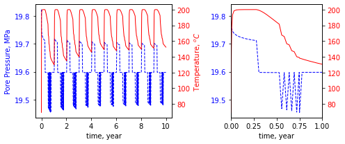
Figure 2: Pore pressure and temperature evolution at the middle of the hot well for the scenario of injection-storage-extraction-rest seasonal cycle of 10 years operation. Note that the extraction operation only occurs when the temperature of the fluid in the hot well ( $var element = document.getElementById("moose-equation-fce86961-3a52-4ad8-bef1-5c7d77ff0fdd");katex.render("T_{hot}", element, {displayMode:false,throwOnError:false});$ ) exceeds the cut-off temperature (i.e., $var element = document.getElementById("moose-equation-4c68b2ed-cae8-40a7-a21f-203525a8fbb9");katex.render("(T_{hot}-T_0)/(T_i-T_0)\\geq 80\\%", element, {displayMode:false,throwOnError:false});$ ), and the hot well temperature can raise again due to heat conduction when extraction stops. This temperature raise will restart the extraction which results in a zigzag-shaped curve during the extraction season as shown above. Note the temperature of the extracted fluid from the hot well has a discrepancy with the temperature at the middle of the well.

Figure 3 shows the histograms of the formation parameters (green) and the operating conditions (magenta) of all the realized simulations. The screening-out process of the physically meaningless cases and the unreasonable cases in practice also results in the non-uniform distribution in flow rate and permeability.

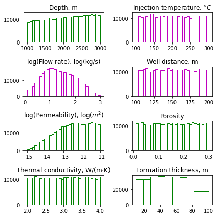
Figure 3: Histograms of the input parameters for all the realized simulations of the seasonal cycle operation. The y-axis stands for the realized simulation numbers after screening. We color-code the formation characteristics in green and the operation conditions in magenta.

Figure 4 plots the histograms of the RTES performance metrics for the seasonal cycle case. Because we stop and restart the extraction process during the winter season according to the fluid temperature in the hot well, the recovery efficiency is high, and the operation time spans from 50 days to 80 days with a close to uniform distribution. The predicted annual storage capacity is close to a power-law distribution, and we plotted it in the logarithmic scale.

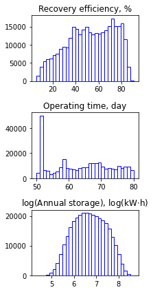
Figure 4: Histograms of the output parameters for all the realized simulations of the seasonal cycle operation.Note the performance metrics are all annual average values.

References

W Jin, R Podgorney, T McLing, and RW Carlsen. Geothermal battery optimization using stochastic hydro-thermal simulations and machine learning algorithms. In 55th US Rock Mechanics/Geomechanics Symposium. OnePetro, 2021.

@inproceedings{jin2021geothermal,
    author = "Jin, W and Podgorney, R and McLing, T and Carlsen, RW",
    title = "Geothermal battery optimization using stochastic hydro-thermal simulations and machine learning algorithms",
    booktitle = "55th US Rock Mechanics/Geomechanics Symposium",
    year = "2021",
    organization = "OnePetro"
}

Wencheng Jin, Trevor Atkinson, Christine Doughty, Ghanashyam Neupane, Nicolas Spycher, Travis McLing, Patrick Dobson, Robert Smith, and Robert Podgorney. Machine-learning-assisted high-temperature reservoir thermal energy storage optimization. Renewable Energy, 2022.

@article{jin2022machine,
    author = "Jin, Wencheng and Atkinson, Trevor and Doughty, Christine and Neupane, Ghanashyam and Spycher, Nicolas and McLing, Travis and Dobson, Patrick and Smith, Robert and Podgorney, Robert",
    title = "Machine-learning-assisted high-temperature reservoir thermal energy storage optimization",
    journal = "Renewable Energy",
    year = "2022",
    publisher = "Elsevier"
}

(examples/rtes_stochastic/base_cycle_50.i)

#---geothermal battery project - looking for sweet spot
#---Define two scalar variables to sweep consistently

depth =  2000
pp_ini_bc = ${fparse if(depth<=2000, 1000*9.8*depth, 1000*9.8*depth+(depth-2000)*9.8*1000)}
T_ini_bc  = ${fparse (80+3.28084*depth*1.1/100-32)*5/9 + 273.15}

distance_between_wells = 200
pro_well_x = ${fparse 0.1 + distance_between_wells / 2}
inj_well_x  = ${fparse 0.1 - distance_between_wells / 2}
well_length = 50  #fixed number in accordance with the mesh
aquifer_mid= ${fparse 0 + 0}
aquifer_top= ${fparse 0 + well_length/2}
aquifer_bot= ${fparse 0 - well_length/2}
#---Define a scalar variable to sweep
inj_ext_exponent = 1.5
inj_ext_flux= ${fparse 10^inj_ext_exponent / well_length / 2 }

injection_temp = 473.15

#---Define a scalar variable to replace the tensor components
Tcond_aquifer = 2.0
#---Define a scalar variable to replace the tensor components
perm_exponent = -12
perm_aquifer = ${fparse 10^perm_exponent}

[Controls]
  [summer_injection]
    type = ConditionalFunctionEnableControl
    conditional_function = inj_function_summer
    enable_objects  = 'DiracKernel::charge_injection_P DiracKernel::charge_injection_T DiracKernel::charge_production_P DiracKernel::charge_production_T'
  []
  [winter_injection]
    type = ConditionalFunctionEnableControl
    conditional_function = inj_function_winter
    enable_objects  = 'DiracKernel::recover_injection_P DiracKernel::recover_injection_T DiracKernel::recover_production_P DiracKernel::recover_production_T'
  []
  [rest_injection]
    type = ConditionalFunctionEnableControl
    conditional_function = rest_function
    enable_objects  = 'DiracKernel::rest_injection_P DiracKernel::rest_injection_T DiracKernel::rest_production_P DiracKernel::rest_production_T'
  []
[]

[Functions]
  [./inj_function_summer]
    type = ParsedFunction
    value = '(t/24/3600/365.25-floor(t/24/3600/365.25))>0 & (t/24/3600/365.25-floor(t/24/3600/365.25))<=0.25'
  [../]
  [./inj_function_winter]
    type = ParsedFunction
    vals = 'termination'
    vars = 'b_switch'
    value = '((t/24/3600/365.25-floor(t/24/3600/365.25))>0.5 & (t/24/3600/365.25-floor(t/24/3600/365.25)) <=0.75) & b_switch <= 0'
  [../]
  [./rest_function]
    type = ParsedFunction
    vals = 'termination'
    vars = 'b_switch'
    value = '(((t/24/3600/365.25-floor(t/24/3600/365.25))>0.25 & (t/24/3600/365.25-floor(t/24/3600/365.25)) <=0.5) | ((t/24/3600/365.25-floor(t/24/3600/365.25))>0.75 & (t/24/3600/365.25-floor(t/24/3600/365.25)) <=1)) | (((t/24/3600/365.25-floor(t/24/3600/365.25))>0.5 & (t/24/3600/365.25-floor(t/24/3600/365.25)) <=0.75) & b_switch >=1)'
  [../]
  [./Fiss_Function]
    type = PiecewiseLinear
    x ='0.            7889400.      15778800.     23668200.
      31557600.     39447000.     47336400.     55225800.
      63115200.     71004600.     78894000.     86783400.
      94672800.     102562200.    110451600.    118341000.
      126230400.    134119800.    142009200.    149898600.
      157788000.    165677400.    173566800.    181456200.
      189345600.    197235000.    205124400.    213013800.
      220903200.    228792600.    236682000.    244571400.
      252460800.    260350200.    268239600.    276129000.
      284018400.    291907800.    299797200.    307686600.
      315576000.'
    y = '0 1  2  3  4
        1 2 3 4
        1 2 3 4
        1 2 3 4
        1 2 3 4
        1 2 3 4
        1 2 3 4
        1 2 3 4
        1 2 3 4
        1 2 3 4'
  [../]
[]

# Darcy flow with heat advection and conduction
[Mesh]
  [./fmg]
    type = FileMeshGenerator
    file = base_final_50.e
  []
[]
#############################################################
[GlobalParams]
  PorousFlowDictator = dictator
[]
############################################################
[PorousFlowUnsaturated]
  relative_permeability_type = COREY
  relative_permeability_exponent = 0
  add_darcy_aux = true
  coupling_type = ThermoHydro
  gravity = '0 0 -9.8'
  porepressure = porepressure
  temperature = temperature
  fp = tabulated_water
  use_displaced_mesh = false
[]
###########################################################
[Variables]
  [./porepressure]
  [../]
  [./temperature]
    scaling = 1E-6
  [../]
[]
###########################################################
[AuxVariables]
  [./density]
    order = CONSTANT
    family = MONOMIAL
  [../]
[]
##############################################################
[AuxKernels]
  [./density]
    type = MaterialRealAux
    variable = density
    property = PorousFlow_fluid_phase_density_qp0
    execute_on = TIMESTEP_END
  [../]
[]
############################################################
[UserObjects]
  [./fluid_mass_in_inc]
    type = PorousFlowSumQuantity
  [../]
  [./fluid_mass_out_inc]
    type = PorousFlowSumQuantity
  [../]
  [./heat_enthalpy_in_inc]
    type = PorousFlowSumQuantity
  [../]
  [./heat_enthalpy_out_inc]
    type = PorousFlowSumQuantity
  [../]
[]

############################################################
[ICs]
  [./init_pp]
    type = FunctionIC
    function = ${pp_ini_bc}
    variable = porepressure
  [../]
  [./init_temp]
    type = ConstantIC
    value = ${T_ini_bc}
    variable = temperature
  [../]
[]
###############################################################
[BCs]
  [./P_drained]
    type = DirichletBC
    variable = porepressure
    boundary = 'east west north'
    value = ${pp_ini_bc}
  [../]
  [./T_cont]
    type = DirichletBC
    variable = temperature
    boundary = 'east west north'
    value = ${T_ini_bc}
  [../]
[]

############################################################
[DiracKernels]
  [./charge_injection_P]
    type = PorousFlowPolyLineSink
    fluid_phase = 0
    variable = porepressure
    SumQuantityUO = fluid_mass_in_inc
    line_base = '1 ${inj_well_x} 0 ${aquifer_bot}'
    line_length = ${well_length}
    line_direction = '0 0 1'
    p_or_t_vals = '-1e9 1e9'
    fluxes = '-${inj_ext_flux} -${inj_ext_flux}'  # ~5 kg/s over length of 10(injection_length)/2
  [../]
  [./charge_injection_T]
    type = EnthalpySink
    fluid_phase = 0
    variable = temperature
    SumQuantityUO = heat_enthalpy_in_inc
    line_base = '1 ${inj_well_x} 0 ${aquifer_bot}'
    line_length = ${well_length}
    line_direction = '0 0 1'
    pressure = porepressure
    T_in = ${injection_temp}
    fp = tabulated_water
    p_or_t_vals = '-1e9 1e9'
    fluxes = '-${inj_ext_flux} -${inj_ext_flux}'
  [../]
  [./charge_production_P]
    type = PorousFlowPolyLineSink
    fluid_phase = 0
    variable = porepressure
    SumQuantityUO = fluid_mass_out_inc
    line_base = '1 ${pro_well_x} 0 ${aquifer_bot}'
    line_length = ${well_length}
    line_direction = '0 0 1'
    p_or_t_vals = '-1e9 1e9'
    fluxes = '${inj_ext_flux} ${inj_ext_flux}'
  [../]
  [./charge_production_T]
    type = PorousFlowPolyLineSink
    fluid_phase = 0
    variable = temperature
    SumQuantityUO = heat_enthalpy_out_inc
    line_base = '1 ${pro_well_x} 0 ${aquifer_bot}'
    line_length = ${well_length}
    line_direction = '0 0 1'
    use_enthalpy = true
    p_or_t_vals = '-1e9 1e9'
    fluxes = '${inj_ext_flux} ${inj_ext_flux}'
  [../]

  [./recover_production_P]
    type = PorousFlowPolyLineSink
    fluid_phase = 0
    variable = porepressure
    SumQuantityUO = fluid_mass_in_inc
    line_base = '1 ${inj_well_x} 0 ${aquifer_bot}'
    line_length = ${well_length}
    line_direction = '0 0 1'
    p_or_t_vals = '-1e9 1e9'
    fluxes = '${inj_ext_flux} ${inj_ext_flux}'  # ~5 kg/s over length of 10(injection_length)/2
  [../]
  [./recover_production_T]
    type = PorousFlowPolyLineSink
    fluid_phase = 0
    variable = temperature
    SumQuantityUO = heat_enthalpy_in_inc
    line_base = '1 ${inj_well_x} 0 ${aquifer_bot}'
    line_length = ${well_length}
    line_direction = '0 0 1'
    use_enthalpy = true
    p_or_t_vals = '-1e9 1e9'
    fluxes = '${inj_ext_flux} ${inj_ext_flux}'
  [../]
  [./recover_injection_P]
    type = PorousFlowPolyLineSink
    fluid_phase = 0
    variable = porepressure
    SumQuantityUO = fluid_mass_out_inc
    line_base = '1 ${pro_well_x} 0 ${aquifer_bot}'
    line_length = ${well_length}
    line_direction = '0 0 1'
    p_or_t_vals = '-1e9 1e9'
    fluxes = '-${inj_ext_flux} -${inj_ext_flux}'
  [../]
  [./recover_injection_T]
    type = EnthalpySink
    fluid_phase = 0
    variable = temperature
    SumQuantityUO = heat_enthalpy_out_inc
    line_base = '1 ${pro_well_x} 0 ${aquifer_bot}'
    line_length = ${well_length}
    line_direction = '0 0 1'
    pressure = porepressure
    T_in = ${T_ini_bc}
    fp = tabulated_water
    p_or_t_vals = '-1e9 1e9'
    fluxes = '-${inj_ext_flux} -${inj_ext_flux}'
  [../]

[./rest_production_P]
    type = PorousFlowPolyLineSink
    fluid_phase = 0
    variable = porepressure
    SumQuantityUO = fluid_mass_in_inc
    line_base = '1 ${inj_well_x} 0 ${aquifer_bot}'
    line_length = ${well_length}
    line_direction = '0 0 1'
    p_or_t_vals = '-1e9 1e9'
    fluxes = '0 0'  # ~5 kg/s over length of 10(injection_length)/2
  [../]
  [./rest_production_T]
    type = PorousFlowPolyLineSink
    fluid_phase = 0
    variable = temperature
    SumQuantityUO = heat_enthalpy_in_inc
    line_base = '1 ${inj_well_x} 0 ${aquifer_bot}'
    line_length = ${well_length}
    line_direction = '0 0 1'
    use_enthalpy = true
    p_or_t_vals = '-1e9 1e9'
    fluxes = '0 0'
  [../]
  [./rest_injection_P]
    type = PorousFlowPolyLineSink
    fluid_phase = 0
    variable = porepressure
    SumQuantityUO = fluid_mass_out_inc
    line_base = '1 ${pro_well_x} 0 ${aquifer_bot}'
    line_length = ${well_length}
    line_direction = '0 0 1'
    p_or_t_vals = '-1e9 1e9'
    fluxes = '0 0'
  [../]
  [./rest_injection_T]
    type = EnthalpySink
    fluid_phase = 0
    variable = temperature
    SumQuantityUO = heat_enthalpy_out_inc
    line_base = '1 ${pro_well_x} 0 ${aquifer_bot}'
    line_length = ${well_length}
    line_direction = '0 0 1'
    pressure = porepressure
    T_in = ${T_ini_bc}
    fp = tabulated_water
    p_or_t_vals = '-1e9 1e9'
    fluxes = '0 0'
  [../]




[]
############################################################
[Modules]
  [./FluidProperties]
    [./true_water]
      type = Water97FluidProperties
    [../]
    [./tabulated_water]
      type = TabulatedFluidProperties
      fp = true_water
      temperature_min = 275
      temperature_max = 600
      pressure_max = 1E8
      interpolated_properties = 'density viscosity enthalpy internal_energy'
      fluid_property_file = water97_tabulated.csv
    [../]
  [../]
[]
############################################################
[Materials]
  [./internal_energy_aquifer]
    type = PorousFlowMatrixInternalEnergy
    specific_heat_capacity = 930.0
    density = 2650.0
    block = 'aquifer_HEX8 aquifer_WEDGE'
  [../]
  [./thermal_conductivity_aquifer]
    type = PorousFlowThermalConductivityIdeal
    dry_thermal_conductivity = '${Tcond_aquifer} 0 0  0 ${Tcond_aquifer} 0  0 0 ${Tcond_aquifer}'
    block = 'aquifer_HEX8 aquifer_WEDGE'
  [../]
  [./porosity_aquifer]
    type = PorousFlowPorosityConst
    block = 'aquifer_HEX8 aquifer_WEDGE'
    porosity = 0.01
  [../]
  [./permeability_aquifer]
    type = PorousFlowPermeabilityConst
    block = 'aquifer_HEX8 aquifer_WEDGE'
    permeability = '${perm_aquifer} 0 0   0 ${perm_aquifer} 0   0 0 ${perm_aquifer}'
  [../]
  [./internal_energy_caps]
    type = PorousFlowMatrixInternalEnergy
    specific_heat_capacity = 1000.0
    density = 2500.0
    block = 'caps_HEX8 caps_WEDGE'
  [../]
  [./thermal_conductivity_caps]
    type = PorousFlowThermalConductivityIdeal
    dry_thermal_conductivity = '2.5 0 0  0 2.5 0  0 0 2.5'
    block = 'caps_HEX8 caps_WEDGE'
  [../]
  [./porosity_caps]
    type = PorousFlowPorosityConst
    block = 'caps_HEX8 caps_WEDGE'
    porosity = 0.01
  [../]
  [./permeability_caps]
    type = PorousFlowPermeabilityConst
    block = 'caps_HEX8 caps_WEDGE'
    permeability = '1E-18 0 0   0 1E-18 0   0 0 1E-18'
  [../]
[]
############################################################
[Preconditioning]
active = 'ilu_may_use_less_mem'
#active = 'superlu'

[./ilu_may_use_less_mem]
type = SMP
full = true
petsc_options = '-ksp_diagonal_scale -ksp_diagonal_scale_fix'
petsc_options_iname = '-ksp_type -pc_type -sub_pc_type -sub_pc_factor_shift_type -sub_pc_factor_levels'
petsc_options_value = 'gmres asm ilu NONZERO 2'
[../]

[./original]
type = SMP
full = true
petsc_options = '-ksp_diagonal_scale -ksp_diagonal_scale_fix'
petsc_options_iname = '-ksp_type -pc_type -sub_pc_type -sub_pc_factor_shift_type'
petsc_options_value = 'gmres asm lu NONZERO'
[../]

[./superlu]
type = SMP
full = true
petsc_options = '-ksp_diagonal_scale -ksp_diagonal_scale_fix'
petsc_options_iname = '-ksp_type -pc_type -pc_factor_mat_solver_package'
petsc_options_value = 'gmres lu superlu_dist'
[../]

[./sub_pc_superlu]
type = SMP
full = true
petsc_options = '-ksp_diagonal_scale -ksp_diagonal_scale_fix'
petsc_options_iname = '-ksp_type -pc_type -sub_pc_type -sub_pc_factor_shift_type -sub_pc_factor_mat_solver_package'
petsc_options_value = 'gmres asm lu NONZERO superlu_dist'
[../]

[./preferred]
#per Andy
type = SMP
full = true
petsc_options_iname = '-pc_type -pc_factor_mat_solver_package'
petsc_options_value = ' lu       mumps'
[../]

[./basic]
type = SMP
full = true
petsc_options = '-ksp_diagonal_scale -ksp_diagonal_scale_fix'
petsc_options_iname = '-pc_type -sub_pc_type -sub_pc_factor_shift_type -pc_asm_overlap'
petsc_options_value = ' asm      lu           NONZERO                   2'
[../]

[]

############################################################

[Postprocessors]
  [./hotwell_mass_kg]
    type = PorousFlowPlotQuantity
    uo = fluid_mass_in_inc
  [../]
  [./hotwell_enthalpy_J]
    type = PorousFlowPlotQuantity
    uo = heat_enthalpy_in_inc
  [../]
  [./coldwell_mass_kg]
    type = PorousFlowPlotQuantity
    uo = fluid_mass_out_inc
  [../]
  [./coldwell_enthalpy_J]
    type = PorousFlowPlotQuantity
    uo = heat_enthalpy_out_inc
  [../]

  [./time]
    type = TimePostprocessor
    execute_on = 'timestep_end'
  []
  [./step_dt]
    type = TimestepSize
  [../]

  [./is_winter]
    type = FunctionValuePostprocessor
    function = inj_function_winter
  [../]
  [./is_summer]
    type = FunctionValuePostprocessor
    function = inj_function_summer
  [../]


  [./total_recovery_time]
    type = PorousFlowRecoveryTimeAccumulator
    targetpostprocessor = is_winter
    dtpostprocessor = step_dt
  [../]

  [./termination]
    type = PorousFlowTemperatureDropTerminator
    enthalpypostprocessor = hotwell_enthalpy_J
    masspostprocessor = hotwell_mass_kg
    T_inj = ${injection_temp}
    T_init = ${T_ini_bc}
    P_drop = 80
    timepostprocessor = time
  [../]

  [./recovery_rate]
    type = PorousFlowRecoveryRateSeason
    hotwellenergy = hotwell_enthalpy_J
    coldwellenergy = coldwell_enthalpy_J
    InjectionIndicator = is_summer
    ProductionIndicator = is_winter
  [../]

  [./total_energy]
    type = PorousFlowEnergyAccumulator
    hotwellenergy = hotwell_enthalpy_J
    coldwellenergy = coldwell_enthalpy_J
    ProductionIndicator = is_winter
  [../]

  [./inj_P_mid]
    type = PointValue
    execute_on = 'initial timestep_end'
    point = '${inj_well_x} 0 ${aquifer_mid}'
    variable = porepressure
  [../]
  [./inj_T_mid]
    type = PointValue
    execute_on = 'initial timestep_end'
    point = '${inj_well_x} 0 ${aquifer_mid}'
    variable = temperature
  [../]
  [./pro_P_mid]
    type = PointValue
    execute_on = 'initial timestep_end'
    point = '${pro_well_x} 0 ${aquifer_mid}'
    variable = porepressure
  [../]
  [./pro_T_mid]
    type = PointValue
    execute_on = 'initial timestep_end'
    point = '${pro_well_x} 0 ${aquifer_mid}'
    variable = temperature
  [../]
[]

##########################################################
[Executioner]
  type = Transient
  solve_type = NEWTON
  end_time = 315576000
#  steady_state_detection = true
#  steady_state_start_time = 864000 # 10 days
#  steady_state_tolerance = 1e-6
  dtmax = 864000 # 10 days
  dtmin = 100
 [./TimeStepper]
   type = IterationAdaptiveDT
   dt = 1000.0
   optimal_iterations = 10
   force_step_every_function_point =  true
   timestep_limiting_function = Fiss_Function
#  timestep_limiting_postprocessor = timestep_pp
 [../]
# controls for linear iterations
  l_max_its = 50
  l_tol = 1e-3
# controls for nonlinear iterations
  nl_max_its = 20
  nl_rel_tol = 1e-5
  nl_abs_tol = 1e-4
[]
###########################################################
[Outputs]



#[./exodus]
#    type = Exodus
#    file_base = sequence_out_1
#    elemental_as_nodal = true
#    overwrite = true
#    sequence = true
#     interval = 2
#[../]

#[./Console]
#  type = Console
#  #perf_log = false
#  #output_linear = true
#  output_nonlinear = true
#  interval = 1
#[../]

[./CSV]
  type = CSV
  interval = 1
[../]
[]
###########################################################

(examples/rtes_stochastic/base_cycle_50.i)

#---geothermal battery project - looking for sweet spot
#---Define two scalar variables to sweep consistently

depth =  2000
pp_ini_bc = ${fparse if(depth<=2000, 1000*9.8*depth, 1000*9.8*depth+(depth-2000)*9.8*1000)}
T_ini_bc  = ${fparse (80+3.28084*depth*1.1/100-32)*5/9 + 273.15}

distance_between_wells = 200
pro_well_x = ${fparse 0.1 + distance_between_wells / 2}
inj_well_x  = ${fparse 0.1 - distance_between_wells / 2}
well_length = 50  #fixed number in accordance with the mesh
aquifer_mid= ${fparse 0 + 0}
aquifer_top= ${fparse 0 + well_length/2}
aquifer_bot= ${fparse 0 - well_length/2}
#---Define a scalar variable to sweep
inj_ext_exponent = 1.5
inj_ext_flux= ${fparse 10^inj_ext_exponent / well_length / 2 }

injection_temp = 473.15

#---Define a scalar variable to replace the tensor components
Tcond_aquifer = 2.0
#---Define a scalar variable to replace the tensor components
perm_exponent = -12
perm_aquifer = ${fparse 10^perm_exponent}

[Controls]
  [summer_injection]
    type = ConditionalFunctionEnableControl
    conditional_function = inj_function_summer
    enable_objects  = 'DiracKernel::charge_injection_P DiracKernel::charge_injection_T DiracKernel::charge_production_P DiracKernel::charge_production_T'
  []
  [winter_injection]
    type = ConditionalFunctionEnableControl
    conditional_function = inj_function_winter
    enable_objects  = 'DiracKernel::recover_injection_P DiracKernel::recover_injection_T DiracKernel::recover_production_P DiracKernel::recover_production_T'
  []
  [rest_injection]
    type = ConditionalFunctionEnableControl
    conditional_function = rest_function
    enable_objects  = 'DiracKernel::rest_injection_P DiracKernel::rest_injection_T DiracKernel::rest_production_P DiracKernel::rest_production_T'
  []
[]

[Functions]
  [./inj_function_summer]
    type = ParsedFunction
    value = '(t/24/3600/365.25-floor(t/24/3600/365.25))>0 & (t/24/3600/365.25-floor(t/24/3600/365.25))<=0.25'
  [../]
  [./inj_function_winter]
    type = ParsedFunction
    vals = 'termination'
    vars = 'b_switch'
    value = '((t/24/3600/365.25-floor(t/24/3600/365.25))>0.5 & (t/24/3600/365.25-floor(t/24/3600/365.25)) <=0.75) & b_switch <= 0'
  [../]
  [./rest_function]
    type = ParsedFunction
    vals = 'termination'
    vars = 'b_switch'
    value = '(((t/24/3600/365.25-floor(t/24/3600/365.25))>0.25 & (t/24/3600/365.25-floor(t/24/3600/365.25)) <=0.5) | ((t/24/3600/365.25-floor(t/24/3600/365.25))>0.75 & (t/24/3600/365.25-floor(t/24/3600/365.25)) <=1)) | (((t/24/3600/365.25-floor(t/24/3600/365.25))>0.5 & (t/24/3600/365.25-floor(t/24/3600/365.25)) <=0.75) & b_switch >=1)'
  [../]
  [./Fiss_Function]
    type = PiecewiseLinear
    x ='0.            7889400.      15778800.     23668200.
      31557600.     39447000.     47336400.     55225800.
      63115200.     71004600.     78894000.     86783400.
      94672800.     102562200.    110451600.    118341000.
      126230400.    134119800.    142009200.    149898600.
      157788000.    165677400.    173566800.    181456200.
      189345600.    197235000.    205124400.    213013800.
      220903200.    228792600.    236682000.    244571400.
      252460800.    260350200.    268239600.    276129000.
      284018400.    291907800.    299797200.    307686600.
      315576000.'
    y = '0 1  2  3  4
        1 2 3 4
        1 2 3 4
        1 2 3 4
        1 2 3 4
        1 2 3 4
        1 2 3 4
        1 2 3 4
        1 2 3 4
        1 2 3 4'
  [../]
[]

# Darcy flow with heat advection and conduction
[Mesh]
  [./fmg]
    type = FileMeshGenerator
    file = base_final_50.e
  []
[]
#############################################################
[GlobalParams]
  PorousFlowDictator = dictator
[]
############################################################
[PorousFlowUnsaturated]
  relative_permeability_type = COREY
  relative_permeability_exponent = 0
  add_darcy_aux = true
  coupling_type = ThermoHydro
  gravity = '0 0 -9.8'
  porepressure = porepressure
  temperature = temperature
  fp = tabulated_water
  use_displaced_mesh = false
[]
###########################################################
[Variables]
  [./porepressure]
  [../]
  [./temperature]
    scaling = 1E-6
  [../]
[]
###########################################################
[AuxVariables]
  [./density]
    order = CONSTANT
    family = MONOMIAL
  [../]
[]
##############################################################
[AuxKernels]
  [./density]
    type = MaterialRealAux
    variable = density
    property = PorousFlow_fluid_phase_density_qp0
    execute_on = TIMESTEP_END
  [../]
[]
############################################################
[UserObjects]
  [./fluid_mass_in_inc]
    type = PorousFlowSumQuantity
  [../]
  [./fluid_mass_out_inc]
    type = PorousFlowSumQuantity
  [../]
  [./heat_enthalpy_in_inc]
    type = PorousFlowSumQuantity
  [../]
  [./heat_enthalpy_out_inc]
    type = PorousFlowSumQuantity
  [../]
[]

############################################################
[ICs]
  [./init_pp]
    type = FunctionIC
    function = ${pp_ini_bc}
    variable = porepressure
  [../]
  [./init_temp]
    type = ConstantIC
    value = ${T_ini_bc}
    variable = temperature
  [../]
[]
###############################################################
[BCs]
  [./P_drained]
    type = DirichletBC
    variable = porepressure
    boundary = 'east west north'
    value = ${pp_ini_bc}
  [../]
  [./T_cont]
    type = DirichletBC
    variable = temperature
    boundary = 'east west north'
    value = ${T_ini_bc}
  [../]
[]

############################################################
[DiracKernels]
  [./charge_injection_P]
    type = PorousFlowPolyLineSink
    fluid_phase = 0
    variable = porepressure
    SumQuantityUO = fluid_mass_in_inc
    line_base = '1 ${inj_well_x} 0 ${aquifer_bot}'
    line_length = ${well_length}
    line_direction = '0 0 1'
    p_or_t_vals = '-1e9 1e9'
    fluxes = '-${inj_ext_flux} -${inj_ext_flux}'  # ~5 kg/s over length of 10(injection_length)/2
  [../]
  [./charge_injection_T]
    type = EnthalpySink
    fluid_phase = 0
    variable = temperature
    SumQuantityUO = heat_enthalpy_in_inc
    line_base = '1 ${inj_well_x} 0 ${aquifer_bot}'
    line_length = ${well_length}
    line_direction = '0 0 1'
    pressure = porepressure
    T_in = ${injection_temp}
    fp = tabulated_water
    p_or_t_vals = '-1e9 1e9'
    fluxes = '-${inj_ext_flux} -${inj_ext_flux}'
  [../]
  [./charge_production_P]
    type = PorousFlowPolyLineSink
    fluid_phase = 0
    variable = porepressure
    SumQuantityUO = fluid_mass_out_inc
    line_base = '1 ${pro_well_x} 0 ${aquifer_bot}'
    line_length = ${well_length}
    line_direction = '0 0 1'
    p_or_t_vals = '-1e9 1e9'
    fluxes = '${inj_ext_flux} ${inj_ext_flux}'
  [../]
  [./charge_production_T]
    type = PorousFlowPolyLineSink
    fluid_phase = 0
    variable = temperature
    SumQuantityUO = heat_enthalpy_out_inc
    line_base = '1 ${pro_well_x} 0 ${aquifer_bot}'
    line_length = ${well_length}
    line_direction = '0 0 1'
    use_enthalpy = true
    p_or_t_vals = '-1e9 1e9'
    fluxes = '${inj_ext_flux} ${inj_ext_flux}'
  [../]

  [./recover_production_P]
    type = PorousFlowPolyLineSink
    fluid_phase = 0
    variable = porepressure
    SumQuantityUO = fluid_mass_in_inc
    line_base = '1 ${inj_well_x} 0 ${aquifer_bot}'
    line_length = ${well_length}
    line_direction = '0 0 1'
    p_or_t_vals = '-1e9 1e9'
    fluxes = '${inj_ext_flux} ${inj_ext_flux}'  # ~5 kg/s over length of 10(injection_length)/2
  [../]
  [./recover_production_T]
    type = PorousFlowPolyLineSink
    fluid_phase = 0
    variable = temperature
    SumQuantityUO = heat_enthalpy_in_inc
    line_base = '1 ${inj_well_x} 0 ${aquifer_bot}'
    line_length = ${well_length}
    line_direction = '0 0 1'
    use_enthalpy = true
    p_or_t_vals = '-1e9 1e9'
    fluxes = '${inj_ext_flux} ${inj_ext_flux}'
  [../]
  [./recover_injection_P]
    type = PorousFlowPolyLineSink
    fluid_phase = 0
    variable = porepressure
    SumQuantityUO = fluid_mass_out_inc
    line_base = '1 ${pro_well_x} 0 ${aquifer_bot}'
    line_length = ${well_length}
    line_direction = '0 0 1'
    p_or_t_vals = '-1e9 1e9'
    fluxes = '-${inj_ext_flux} -${inj_ext_flux}'
  [../]
  [./recover_injection_T]
    type = EnthalpySink
    fluid_phase = 0
    variable = temperature
    SumQuantityUO = heat_enthalpy_out_inc
    line_base = '1 ${pro_well_x} 0 ${aquifer_bot}'
    line_length = ${well_length}
    line_direction = '0 0 1'
    pressure = porepressure
    T_in = ${T_ini_bc}
    fp = tabulated_water
    p_or_t_vals = '-1e9 1e9'
    fluxes = '-${inj_ext_flux} -${inj_ext_flux}'
  [../]

[./rest_production_P]
    type = PorousFlowPolyLineSink
    fluid_phase = 0
    variable = porepressure
    SumQuantityUO = fluid_mass_in_inc
    line_base = '1 ${inj_well_x} 0 ${aquifer_bot}'
    line_length = ${well_length}
    line_direction = '0 0 1'
    p_or_t_vals = '-1e9 1e9'
    fluxes = '0 0'  # ~5 kg/s over length of 10(injection_length)/2
  [../]
  [./rest_production_T]
    type = PorousFlowPolyLineSink
    fluid_phase = 0
    variable = temperature
    SumQuantityUO = heat_enthalpy_in_inc
    line_base = '1 ${inj_well_x} 0 ${aquifer_bot}'
    line_length = ${well_length}
    line_direction = '0 0 1'
    use_enthalpy = true
    p_or_t_vals = '-1e9 1e9'
    fluxes = '0 0'
  [../]
  [./rest_injection_P]
    type = PorousFlowPolyLineSink
    fluid_phase = 0
    variable = porepressure
    SumQuantityUO = fluid_mass_out_inc
    line_base = '1 ${pro_well_x} 0 ${aquifer_bot}'
    line_length = ${well_length}
    line_direction = '0 0 1'
    p_or_t_vals = '-1e9 1e9'
    fluxes = '0 0'
  [../]
  [./rest_injection_T]
    type = EnthalpySink
    fluid_phase = 0
    variable = temperature
    SumQuantityUO = heat_enthalpy_out_inc
    line_base = '1 ${pro_well_x} 0 ${aquifer_bot}'
    line_length = ${well_length}
    line_direction = '0 0 1'
    pressure = porepressure
    T_in = ${T_ini_bc}
    fp = tabulated_water
    p_or_t_vals = '-1e9 1e9'
    fluxes = '0 0'
  [../]




[]
############################################################
[Modules]
  [./FluidProperties]
    [./true_water]
      type = Water97FluidProperties
    [../]
    [./tabulated_water]
      type = TabulatedFluidProperties
      fp = true_water
      temperature_min = 275
      temperature_max = 600
      pressure_max = 1E8
      interpolated_properties = 'density viscosity enthalpy internal_energy'
      fluid_property_file = water97_tabulated.csv
    [../]
  [../]
[]
############################################################
[Materials]
  [./internal_energy_aquifer]
    type = PorousFlowMatrixInternalEnergy
    specific_heat_capacity = 930.0
    density = 2650.0
    block = 'aquifer_HEX8 aquifer_WEDGE'
  [../]
  [./thermal_conductivity_aquifer]
    type = PorousFlowThermalConductivityIdeal
    dry_thermal_conductivity = '${Tcond_aquifer} 0 0  0 ${Tcond_aquifer} 0  0 0 ${Tcond_aquifer}'
    block = 'aquifer_HEX8 aquifer_WEDGE'
  [../]
  [./porosity_aquifer]
    type = PorousFlowPorosityConst
    block = 'aquifer_HEX8 aquifer_WEDGE'
    porosity = 0.01
  [../]
  [./permeability_aquifer]
    type = PorousFlowPermeabilityConst
    block = 'aquifer_HEX8 aquifer_WEDGE'
    permeability = '${perm_aquifer} 0 0   0 ${perm_aquifer} 0   0 0 ${perm_aquifer}'
  [../]
  [./internal_energy_caps]
    type = PorousFlowMatrixInternalEnergy
    specific_heat_capacity = 1000.0
    density = 2500.0
    block = 'caps_HEX8 caps_WEDGE'
  [../]
  [./thermal_conductivity_caps]
    type = PorousFlowThermalConductivityIdeal
    dry_thermal_conductivity = '2.5 0 0  0 2.5 0  0 0 2.5'
    block = 'caps_HEX8 caps_WEDGE'
  [../]
  [./porosity_caps]
    type = PorousFlowPorosityConst
    block = 'caps_HEX8 caps_WEDGE'
    porosity = 0.01
  [../]
  [./permeability_caps]
    type = PorousFlowPermeabilityConst
    block = 'caps_HEX8 caps_WEDGE'
    permeability = '1E-18 0 0   0 1E-18 0   0 0 1E-18'
  [../]
[]
############################################################
[Preconditioning]
active = 'ilu_may_use_less_mem'
#active = 'superlu'

[./ilu_may_use_less_mem]
type = SMP
full = true
petsc_options = '-ksp_diagonal_scale -ksp_diagonal_scale_fix'
petsc_options_iname = '-ksp_type -pc_type -sub_pc_type -sub_pc_factor_shift_type -sub_pc_factor_levels'
petsc_options_value = 'gmres asm ilu NONZERO 2'
[../]

[./original]
type = SMP
full = true
petsc_options = '-ksp_diagonal_scale -ksp_diagonal_scale_fix'
petsc_options_iname = '-ksp_type -pc_type -sub_pc_type -sub_pc_factor_shift_type'
petsc_options_value = 'gmres asm lu NONZERO'
[../]

[./superlu]
type = SMP
full = true
petsc_options = '-ksp_diagonal_scale -ksp_diagonal_scale_fix'
petsc_options_iname = '-ksp_type -pc_type -pc_factor_mat_solver_package'
petsc_options_value = 'gmres lu superlu_dist'
[../]

[./sub_pc_superlu]
type = SMP
full = true
petsc_options = '-ksp_diagonal_scale -ksp_diagonal_scale_fix'
petsc_options_iname = '-ksp_type -pc_type -sub_pc_type -sub_pc_factor_shift_type -sub_pc_factor_mat_solver_package'
petsc_options_value = 'gmres asm lu NONZERO superlu_dist'
[../]

[./preferred]
#per Andy
type = SMP
full = true
petsc_options_iname = '-pc_type -pc_factor_mat_solver_package'
petsc_options_value = ' lu       mumps'
[../]

[./basic]
type = SMP
full = true
petsc_options = '-ksp_diagonal_scale -ksp_diagonal_scale_fix'
petsc_options_iname = '-pc_type -sub_pc_type -sub_pc_factor_shift_type -pc_asm_overlap'
petsc_options_value = ' asm      lu           NONZERO                   2'
[../]

[]

############################################################

[Postprocessors]
  [./hotwell_mass_kg]
    type = PorousFlowPlotQuantity
    uo = fluid_mass_in_inc
  [../]
  [./hotwell_enthalpy_J]
    type = PorousFlowPlotQuantity
    uo = heat_enthalpy_in_inc
  [../]
  [./coldwell_mass_kg]
    type = PorousFlowPlotQuantity
    uo = fluid_mass_out_inc
  [../]
  [./coldwell_enthalpy_J]
    type = PorousFlowPlotQuantity
    uo = heat_enthalpy_out_inc
  [../]

  [./time]
    type = TimePostprocessor
    execute_on = 'timestep_end'
  []
  [./step_dt]
    type = TimestepSize
  [../]

  [./is_winter]
    type = FunctionValuePostprocessor
    function = inj_function_winter
  [../]
  [./is_summer]
    type = FunctionValuePostprocessor
    function = inj_function_summer
  [../]


  [./total_recovery_time]
    type = PorousFlowRecoveryTimeAccumulator
    targetpostprocessor = is_winter
    dtpostprocessor = step_dt
  [../]

  [./termination]
    type = PorousFlowTemperatureDropTerminator
    enthalpypostprocessor = hotwell_enthalpy_J
    masspostprocessor = hotwell_mass_kg
    T_inj = ${injection_temp}
    T_init = ${T_ini_bc}
    P_drop = 80
    timepostprocessor = time
  [../]

  [./recovery_rate]
    type = PorousFlowRecoveryRateSeason
    hotwellenergy = hotwell_enthalpy_J
    coldwellenergy = coldwell_enthalpy_J
    InjectionIndicator = is_summer
    ProductionIndicator = is_winter
  [../]

  [./total_energy]
    type = PorousFlowEnergyAccumulator
    hotwellenergy = hotwell_enthalpy_J
    coldwellenergy = coldwell_enthalpy_J
    ProductionIndicator = is_winter
  [../]

  [./inj_P_mid]
    type = PointValue
    execute_on = 'initial timestep_end'
    point = '${inj_well_x} 0 ${aquifer_mid}'
    variable = porepressure
  [../]
  [./inj_T_mid]
    type = PointValue
    execute_on = 'initial timestep_end'
    point = '${inj_well_x} 0 ${aquifer_mid}'
    variable = temperature
  [../]
  [./pro_P_mid]
    type = PointValue
    execute_on = 'initial timestep_end'
    point = '${pro_well_x} 0 ${aquifer_mid}'
    variable = porepressure
  [../]
  [./pro_T_mid]
    type = PointValue
    execute_on = 'initial timestep_end'
    point = '${pro_well_x} 0 ${aquifer_mid}'
    variable = temperature
  [../]
[]

##########################################################
[Executioner]
  type = Transient
  solve_type = NEWTON
  end_time = 315576000
#  steady_state_detection = true
#  steady_state_start_time = 864000 # 10 days
#  steady_state_tolerance = 1e-6
  dtmax = 864000 # 10 days
  dtmin = 100
 [./TimeStepper]
   type = IterationAdaptiveDT
   dt = 1000.0
   optimal_iterations = 10
   force_step_every_function_point =  true
   timestep_limiting_function = Fiss_Function
#  timestep_limiting_postprocessor = timestep_pp
 [../]
# controls for linear iterations
  l_max_its = 50
  l_tol = 1e-3
# controls for nonlinear iterations
  nl_max_its = 20
  nl_rel_tol = 1e-5
  nl_abs_tol = 1e-4
[]
###########################################################
[Outputs]



#[./exodus]
#    type = Exodus
#    file_base = sequence_out_1
#    elemental_as_nodal = true
#    overwrite = true
#    sequence = true
#     interval = 2
#[../]

#[./Console]
#  type = Console
#  #perf_log = false
#  #output_linear = true
#  output_nonlinear = true
#  interval = 1
#[../]

[./CSV]
  type = CSV
  interval = 1
[../]
[]
###########################################################

(examples/rtes_stochastic/base_cycle_50.i)

#---geothermal battery project - looking for sweet spot
#---Define two scalar variables to sweep consistently

depth =  2000
pp_ini_bc = ${fparse if(depth<=2000, 1000*9.8*depth, 1000*9.8*depth+(depth-2000)*9.8*1000)}
T_ini_bc  = ${fparse (80+3.28084*depth*1.1/100-32)*5/9 + 273.15}

distance_between_wells = 200
pro_well_x = ${fparse 0.1 + distance_between_wells / 2}
inj_well_x  = ${fparse 0.1 - distance_between_wells / 2}
well_length = 50  #fixed number in accordance with the mesh
aquifer_mid= ${fparse 0 + 0}
aquifer_top= ${fparse 0 + well_length/2}
aquifer_bot= ${fparse 0 - well_length/2}
#---Define a scalar variable to sweep
inj_ext_exponent = 1.5
inj_ext_flux= ${fparse 10^inj_ext_exponent / well_length / 2 }

injection_temp = 473.15

#---Define a scalar variable to replace the tensor components
Tcond_aquifer = 2.0
#---Define a scalar variable to replace the tensor components
perm_exponent = -12
perm_aquifer = ${fparse 10^perm_exponent}

[Controls]
  [summer_injection]
    type = ConditionalFunctionEnableControl
    conditional_function = inj_function_summer
    enable_objects  = 'DiracKernel::charge_injection_P DiracKernel::charge_injection_T DiracKernel::charge_production_P DiracKernel::charge_production_T'
  []
  [winter_injection]
    type = ConditionalFunctionEnableControl
    conditional_function = inj_function_winter
    enable_objects  = 'DiracKernel::recover_injection_P DiracKernel::recover_injection_T DiracKernel::recover_production_P DiracKernel::recover_production_T'
  []
  [rest_injection]
    type = ConditionalFunctionEnableControl
    conditional_function = rest_function
    enable_objects  = 'DiracKernel::rest_injection_P DiracKernel::rest_injection_T DiracKernel::rest_production_P DiracKernel::rest_production_T'
  []
[]

[Functions]
  [./inj_function_summer]
    type = ParsedFunction
    value = '(t/24/3600/365.25-floor(t/24/3600/365.25))>0 & (t/24/3600/365.25-floor(t/24/3600/365.25))<=0.25'
  [../]
  [./inj_function_winter]
    type = ParsedFunction
    vals = 'termination'
    vars = 'b_switch'
    value = '((t/24/3600/365.25-floor(t/24/3600/365.25))>0.5 & (t/24/3600/365.25-floor(t/24/3600/365.25)) <=0.75) & b_switch <= 0'
  [../]
  [./rest_function]
    type = ParsedFunction
    vals = 'termination'
    vars = 'b_switch'
    value = '(((t/24/3600/365.25-floor(t/24/3600/365.25))>0.25 & (t/24/3600/365.25-floor(t/24/3600/365.25)) <=0.5) | ((t/24/3600/365.25-floor(t/24/3600/365.25))>0.75 & (t/24/3600/365.25-floor(t/24/3600/365.25)) <=1)) | (((t/24/3600/365.25-floor(t/24/3600/365.25))>0.5 & (t/24/3600/365.25-floor(t/24/3600/365.25)) <=0.75) & b_switch >=1)'
  [../]
  [./Fiss_Function]
    type = PiecewiseLinear
    x ='0.            7889400.      15778800.     23668200.
      31557600.     39447000.     47336400.     55225800.
      63115200.     71004600.     78894000.     86783400.
      94672800.     102562200.    110451600.    118341000.
      126230400.    134119800.    142009200.    149898600.
      157788000.    165677400.    173566800.    181456200.
      189345600.    197235000.    205124400.    213013800.
      220903200.    228792600.    236682000.    244571400.
      252460800.    260350200.    268239600.    276129000.
      284018400.    291907800.    299797200.    307686600.
      315576000.'
    y = '0 1  2  3  4
        1 2 3 4
        1 2 3 4
        1 2 3 4
        1 2 3 4
        1 2 3 4
        1 2 3 4
        1 2 3 4
        1 2 3 4
        1 2 3 4'
  [../]
[]

# Darcy flow with heat advection and conduction
[Mesh]
  [./fmg]
    type = FileMeshGenerator
    file = base_final_50.e
  []
[]
#############################################################
[GlobalParams]
  PorousFlowDictator = dictator
[]
############################################################
[PorousFlowUnsaturated]
  relative_permeability_type = COREY
  relative_permeability_exponent = 0
  add_darcy_aux = true
  coupling_type = ThermoHydro
  gravity = '0 0 -9.8'
  porepressure = porepressure
  temperature = temperature
  fp = tabulated_water
  use_displaced_mesh = false
[]
###########################################################
[Variables]
  [./porepressure]
  [../]
  [./temperature]
    scaling = 1E-6
  [../]
[]
###########################################################
[AuxVariables]
  [./density]
    order = CONSTANT
    family = MONOMIAL
  [../]
[]
##############################################################
[AuxKernels]
  [./density]
    type = MaterialRealAux
    variable = density
    property = PorousFlow_fluid_phase_density_qp0
    execute_on = TIMESTEP_END
  [../]
[]
############################################################
[UserObjects]
  [./fluid_mass_in_inc]
    type = PorousFlowSumQuantity
  [../]
  [./fluid_mass_out_inc]
    type = PorousFlowSumQuantity
  [../]
  [./heat_enthalpy_in_inc]
    type = PorousFlowSumQuantity
  [../]
  [./heat_enthalpy_out_inc]
    type = PorousFlowSumQuantity
  [../]
[]

############################################################
[ICs]
  [./init_pp]
    type = FunctionIC
    function = ${pp_ini_bc}
    variable = porepressure
  [../]
  [./init_temp]
    type = ConstantIC
    value = ${T_ini_bc}
    variable = temperature
  [../]
[]
###############################################################
[BCs]
  [./P_drained]
    type = DirichletBC
    variable = porepressure
    boundary = 'east west north'
    value = ${pp_ini_bc}
  [../]
  [./T_cont]
    type = DirichletBC
    variable = temperature
    boundary = 'east west north'
    value = ${T_ini_bc}
  [../]
[]

############################################################
[DiracKernels]
  [./charge_injection_P]
    type = PorousFlowPolyLineSink
    fluid_phase = 0
    variable = porepressure
    SumQuantityUO = fluid_mass_in_inc
    line_base = '1 ${inj_well_x} 0 ${aquifer_bot}'
    line_length = ${well_length}
    line_direction = '0 0 1'
    p_or_t_vals = '-1e9 1e9'
    fluxes = '-${inj_ext_flux} -${inj_ext_flux}'  # ~5 kg/s over length of 10(injection_length)/2
  [../]
  [./charge_injection_T]
    type = EnthalpySink
    fluid_phase = 0
    variable = temperature
    SumQuantityUO = heat_enthalpy_in_inc
    line_base = '1 ${inj_well_x} 0 ${aquifer_bot}'
    line_length = ${well_length}
    line_direction = '0 0 1'
    pressure = porepressure
    T_in = ${injection_temp}
    fp = tabulated_water
    p_or_t_vals = '-1e9 1e9'
    fluxes = '-${inj_ext_flux} -${inj_ext_flux}'
  [../]
  [./charge_production_P]
    type = PorousFlowPolyLineSink
    fluid_phase = 0
    variable = porepressure
    SumQuantityUO = fluid_mass_out_inc
    line_base = '1 ${pro_well_x} 0 ${aquifer_bot}'
    line_length = ${well_length}
    line_direction = '0 0 1'
    p_or_t_vals = '-1e9 1e9'
    fluxes = '${inj_ext_flux} ${inj_ext_flux}'
  [../]
  [./charge_production_T]
    type = PorousFlowPolyLineSink
    fluid_phase = 0
    variable = temperature
    SumQuantityUO = heat_enthalpy_out_inc
    line_base = '1 ${pro_well_x} 0 ${aquifer_bot}'
    line_length = ${well_length}
    line_direction = '0 0 1'
    use_enthalpy = true
    p_or_t_vals = '-1e9 1e9'
    fluxes = '${inj_ext_flux} ${inj_ext_flux}'
  [../]

  [./recover_production_P]
    type = PorousFlowPolyLineSink
    fluid_phase = 0
    variable = porepressure
    SumQuantityUO = fluid_mass_in_inc
    line_base = '1 ${inj_well_x} 0 ${aquifer_bot}'
    line_length = ${well_length}
    line_direction = '0 0 1'
    p_or_t_vals = '-1e9 1e9'
    fluxes = '${inj_ext_flux} ${inj_ext_flux}'  # ~5 kg/s over length of 10(injection_length)/2
  [../]
  [./recover_production_T]
    type = PorousFlowPolyLineSink
    fluid_phase = 0
    variable = temperature
    SumQuantityUO = heat_enthalpy_in_inc
    line_base = '1 ${inj_well_x} 0 ${aquifer_bot}'
    line_length = ${well_length}
    line_direction = '0 0 1'
    use_enthalpy = true
    p_or_t_vals = '-1e9 1e9'
    fluxes = '${inj_ext_flux} ${inj_ext_flux}'
  [../]
  [./recover_injection_P]
    type = PorousFlowPolyLineSink
    fluid_phase = 0
    variable = porepressure
    SumQuantityUO = fluid_mass_out_inc
    line_base = '1 ${pro_well_x} 0 ${aquifer_bot}'
    line_length = ${well_length}
    line_direction = '0 0 1'
    p_or_t_vals = '-1e9 1e9'
    fluxes = '-${inj_ext_flux} -${inj_ext_flux}'
  [../]
  [./recover_injection_T]
    type = EnthalpySink
    fluid_phase = 0
    variable = temperature
    SumQuantityUO = heat_enthalpy_out_inc
    line_base = '1 ${pro_well_x} 0 ${aquifer_bot}'
    line_length = ${well_length}
    line_direction = '0 0 1'
    pressure = porepressure
    T_in = ${T_ini_bc}
    fp = tabulated_water
    p_or_t_vals = '-1e9 1e9'
    fluxes = '-${inj_ext_flux} -${inj_ext_flux}'
  [../]

[./rest_production_P]
    type = PorousFlowPolyLineSink
    fluid_phase = 0
    variable = porepressure
    SumQuantityUO = fluid_mass_in_inc
    line_base = '1 ${inj_well_x} 0 ${aquifer_bot}'
    line_length = ${well_length}
    line_direction = '0 0 1'
    p_or_t_vals = '-1e9 1e9'
    fluxes = '0 0'  # ~5 kg/s over length of 10(injection_length)/2
  [../]
  [./rest_production_T]
    type = PorousFlowPolyLineSink
    fluid_phase = 0
    variable = temperature
    SumQuantityUO = heat_enthalpy_in_inc
    line_base = '1 ${inj_well_x} 0 ${aquifer_bot}'
    line_length = ${well_length}
    line_direction = '0 0 1'
    use_enthalpy = true
    p_or_t_vals = '-1e9 1e9'
    fluxes = '0 0'
  [../]
  [./rest_injection_P]
    type = PorousFlowPolyLineSink
    fluid_phase = 0
    variable = porepressure
    SumQuantityUO = fluid_mass_out_inc
    line_base = '1 ${pro_well_x} 0 ${aquifer_bot}'
    line_length = ${well_length}
    line_direction = '0 0 1'
    p_or_t_vals = '-1e9 1e9'
    fluxes = '0 0'
  [../]
  [./rest_injection_T]
    type = EnthalpySink
    fluid_phase = 0
    variable = temperature
    SumQuantityUO = heat_enthalpy_out_inc
    line_base = '1 ${pro_well_x} 0 ${aquifer_bot}'
    line_length = ${well_length}
    line_direction = '0 0 1'
    pressure = porepressure
    T_in = ${T_ini_bc}
    fp = tabulated_water
    p_or_t_vals = '-1e9 1e9'
    fluxes = '0 0'
  [../]




[]
############################################################
[Modules]
  [./FluidProperties]
    [./true_water]
      type = Water97FluidProperties
    [../]
    [./tabulated_water]
      type = TabulatedFluidProperties
      fp = true_water
      temperature_min = 275
      temperature_max = 600
      pressure_max = 1E8
      interpolated_properties = 'density viscosity enthalpy internal_energy'
      fluid_property_file = water97_tabulated.csv
    [../]
  [../]
[]
############################################################
[Materials]
  [./internal_energy_aquifer]
    type = PorousFlowMatrixInternalEnergy
    specific_heat_capacity = 930.0
    density = 2650.0
    block = 'aquifer_HEX8 aquifer_WEDGE'
  [../]
  [./thermal_conductivity_aquifer]
    type = PorousFlowThermalConductivityIdeal
    dry_thermal_conductivity = '${Tcond_aquifer} 0 0  0 ${Tcond_aquifer} 0  0 0 ${Tcond_aquifer}'
    block = 'aquifer_HEX8 aquifer_WEDGE'
  [../]
  [./porosity_aquifer]
    type = PorousFlowPorosityConst
    block = 'aquifer_HEX8 aquifer_WEDGE'
    porosity = 0.01
  [../]
  [./permeability_aquifer]
    type = PorousFlowPermeabilityConst
    block = 'aquifer_HEX8 aquifer_WEDGE'
    permeability = '${perm_aquifer} 0 0   0 ${perm_aquifer} 0   0 0 ${perm_aquifer}'
  [../]
  [./internal_energy_caps]
    type = PorousFlowMatrixInternalEnergy
    specific_heat_capacity = 1000.0
    density = 2500.0
    block = 'caps_HEX8 caps_WEDGE'
  [../]
  [./thermal_conductivity_caps]
    type = PorousFlowThermalConductivityIdeal
    dry_thermal_conductivity = '2.5 0 0  0 2.5 0  0 0 2.5'
    block = 'caps_HEX8 caps_WEDGE'
  [../]
  [./porosity_caps]
    type = PorousFlowPorosityConst
    block = 'caps_HEX8 caps_WEDGE'
    porosity = 0.01
  [../]
  [./permeability_caps]
    type = PorousFlowPermeabilityConst
    block = 'caps_HEX8 caps_WEDGE'
    permeability = '1E-18 0 0   0 1E-18 0   0 0 1E-18'
  [../]
[]
############################################################
[Preconditioning]
active = 'ilu_may_use_less_mem'
#active = 'superlu'

[./ilu_may_use_less_mem]
type = SMP
full = true
petsc_options = '-ksp_diagonal_scale -ksp_diagonal_scale_fix'
petsc_options_iname = '-ksp_type -pc_type -sub_pc_type -sub_pc_factor_shift_type -sub_pc_factor_levels'
petsc_options_value = 'gmres asm ilu NONZERO 2'
[../]

[./original]
type = SMP
full = true
petsc_options = '-ksp_diagonal_scale -ksp_diagonal_scale_fix'
petsc_options_iname = '-ksp_type -pc_type -sub_pc_type -sub_pc_factor_shift_type'
petsc_options_value = 'gmres asm lu NONZERO'
[../]

[./superlu]
type = SMP
full = true
petsc_options = '-ksp_diagonal_scale -ksp_diagonal_scale_fix'
petsc_options_iname = '-ksp_type -pc_type -pc_factor_mat_solver_package'
petsc_options_value = 'gmres lu superlu_dist'
[../]

[./sub_pc_superlu]
type = SMP
full = true
petsc_options = '-ksp_diagonal_scale -ksp_diagonal_scale_fix'
petsc_options_iname = '-ksp_type -pc_type -sub_pc_type -sub_pc_factor_shift_type -sub_pc_factor_mat_solver_package'
petsc_options_value = 'gmres asm lu NONZERO superlu_dist'
[../]

[./preferred]
#per Andy
type = SMP
full = true
petsc_options_iname = '-pc_type -pc_factor_mat_solver_package'
petsc_options_value = ' lu       mumps'
[../]

[./basic]
type = SMP
full = true
petsc_options = '-ksp_diagonal_scale -ksp_diagonal_scale_fix'
petsc_options_iname = '-pc_type -sub_pc_type -sub_pc_factor_shift_type -pc_asm_overlap'
petsc_options_value = ' asm      lu           NONZERO                   2'
[../]

[]

############################################################

[Postprocessors]
  [./hotwell_mass_kg]
    type = PorousFlowPlotQuantity
    uo = fluid_mass_in_inc
  [../]
  [./hotwell_enthalpy_J]
    type = PorousFlowPlotQuantity
    uo = heat_enthalpy_in_inc
  [../]
  [./coldwell_mass_kg]
    type = PorousFlowPlotQuantity
    uo = fluid_mass_out_inc
  [../]
  [./coldwell_enthalpy_J]
    type = PorousFlowPlotQuantity
    uo = heat_enthalpy_out_inc
  [../]

  [./time]
    type = TimePostprocessor
    execute_on = 'timestep_end'
  []
  [./step_dt]
    type = TimestepSize
  [../]

  [./is_winter]
    type = FunctionValuePostprocessor
    function = inj_function_winter
  [../]
  [./is_summer]
    type = FunctionValuePostprocessor
    function = inj_function_summer
  [../]


  [./total_recovery_time]
    type = PorousFlowRecoveryTimeAccumulator
    targetpostprocessor = is_winter
    dtpostprocessor = step_dt
  [../]

  [./termination]
    type = PorousFlowTemperatureDropTerminator
    enthalpypostprocessor = hotwell_enthalpy_J
    masspostprocessor = hotwell_mass_kg
    T_inj = ${injection_temp}
    T_init = ${T_ini_bc}
    P_drop = 80
    timepostprocessor = time
  [../]

  [./recovery_rate]
    type = PorousFlowRecoveryRateSeason
    hotwellenergy = hotwell_enthalpy_J
    coldwellenergy = coldwell_enthalpy_J
    InjectionIndicator = is_summer
    ProductionIndicator = is_winter
  [../]

  [./total_energy]
    type = PorousFlowEnergyAccumulator
    hotwellenergy = hotwell_enthalpy_J
    coldwellenergy = coldwell_enthalpy_J
    ProductionIndicator = is_winter
  [../]

  [./inj_P_mid]
    type = PointValue
    execute_on = 'initial timestep_end'
    point = '${inj_well_x} 0 ${aquifer_mid}'
    variable = porepressure
  [../]
  [./inj_T_mid]
    type = PointValue
    execute_on = 'initial timestep_end'
    point = '${inj_well_x} 0 ${aquifer_mid}'
    variable = temperature
  [../]
  [./pro_P_mid]
    type = PointValue
    execute_on = 'initial timestep_end'
    point = '${pro_well_x} 0 ${aquifer_mid}'
    variable = porepressure
  [../]
  [./pro_T_mid]
    type = PointValue
    execute_on = 'initial timestep_end'
    point = '${pro_well_x} 0 ${aquifer_mid}'
    variable = temperature
  [../]
[]

##########################################################
[Executioner]
  type = Transient
  solve_type = NEWTON
  end_time = 315576000
#  steady_state_detection = true
#  steady_state_start_time = 864000 # 10 days
#  steady_state_tolerance = 1e-6
  dtmax = 864000 # 10 days
  dtmin = 100
 [./TimeStepper]
   type = IterationAdaptiveDT
   dt = 1000.0
   optimal_iterations = 10
   force_step_every_function_point =  true
   timestep_limiting_function = Fiss_Function
#  timestep_limiting_postprocessor = timestep_pp
 [../]
# controls for linear iterations
  l_max_its = 50
  l_tol = 1e-3
# controls for nonlinear iterations
  nl_max_its = 20
  nl_rel_tol = 1e-5
  nl_abs_tol = 1e-4
[]
###########################################################
[Outputs]



#[./exodus]
#    type = Exodus
#    file_base = sequence_out_1
#    elemental_as_nodal = true
#    overwrite = true
#    sequence = true
#     interval = 2
#[../]

#[./Console]
#  type = Console
#  #perf_log = false
#  #output_linear = true
#  output_nonlinear = true
#  interval = 1
#[../]

[./CSV]
  type = CSV
  interval = 1
[../]
[]
###########################################################

(examples/rtes_stochastic/base_cycle_50.i)

#---geothermal battery project - looking for sweet spot
#---Define two scalar variables to sweep consistently

depth =  2000
pp_ini_bc = ${fparse if(depth<=2000, 1000*9.8*depth, 1000*9.8*depth+(depth-2000)*9.8*1000)}
T_ini_bc  = ${fparse (80+3.28084*depth*1.1/100-32)*5/9 + 273.15}

distance_between_wells = 200
pro_well_x = ${fparse 0.1 + distance_between_wells / 2}
inj_well_x  = ${fparse 0.1 - distance_between_wells / 2}
well_length = 50  #fixed number in accordance with the mesh
aquifer_mid= ${fparse 0 + 0}
aquifer_top= ${fparse 0 + well_length/2}
aquifer_bot= ${fparse 0 - well_length/2}
#---Define a scalar variable to sweep
inj_ext_exponent = 1.5
inj_ext_flux= ${fparse 10^inj_ext_exponent / well_length / 2 }

injection_temp = 473.15

#---Define a scalar variable to replace the tensor components
Tcond_aquifer = 2.0
#---Define a scalar variable to replace the tensor components
perm_exponent = -12
perm_aquifer = ${fparse 10^perm_exponent}

[Controls]
  [summer_injection]
    type = ConditionalFunctionEnableControl
    conditional_function = inj_function_summer
    enable_objects  = 'DiracKernel::charge_injection_P DiracKernel::charge_injection_T DiracKernel::charge_production_P DiracKernel::charge_production_T'
  []
  [winter_injection]
    type = ConditionalFunctionEnableControl
    conditional_function = inj_function_winter
    enable_objects  = 'DiracKernel::recover_injection_P DiracKernel::recover_injection_T DiracKernel::recover_production_P DiracKernel::recover_production_T'
  []
  [rest_injection]
    type = ConditionalFunctionEnableControl
    conditional_function = rest_function
    enable_objects  = 'DiracKernel::rest_injection_P DiracKernel::rest_injection_T DiracKernel::rest_production_P DiracKernel::rest_production_T'
  []
[]

[Functions]
  [./inj_function_summer]
    type = ParsedFunction
    value = '(t/24/3600/365.25-floor(t/24/3600/365.25))>0 & (t/24/3600/365.25-floor(t/24/3600/365.25))<=0.25'
  [../]
  [./inj_function_winter]
    type = ParsedFunction
    vals = 'termination'
    vars = 'b_switch'
    value = '((t/24/3600/365.25-floor(t/24/3600/365.25))>0.5 & (t/24/3600/365.25-floor(t/24/3600/365.25)) <=0.75) & b_switch <= 0'
  [../]
  [./rest_function]
    type = ParsedFunction
    vals = 'termination'
    vars = 'b_switch'
    value = '(((t/24/3600/365.25-floor(t/24/3600/365.25))>0.25 & (t/24/3600/365.25-floor(t/24/3600/365.25)) <=0.5) | ((t/24/3600/365.25-floor(t/24/3600/365.25))>0.75 & (t/24/3600/365.25-floor(t/24/3600/365.25)) <=1)) | (((t/24/3600/365.25-floor(t/24/3600/365.25))>0.5 & (t/24/3600/365.25-floor(t/24/3600/365.25)) <=0.75) & b_switch >=1)'
  [../]
  [./Fiss_Function]
    type = PiecewiseLinear
    x ='0.            7889400.      15778800.     23668200.
      31557600.     39447000.     47336400.     55225800.
      63115200.     71004600.     78894000.     86783400.
      94672800.     102562200.    110451600.    118341000.
      126230400.    134119800.    142009200.    149898600.
      157788000.    165677400.    173566800.    181456200.
      189345600.    197235000.    205124400.    213013800.
      220903200.    228792600.    236682000.    244571400.
      252460800.    260350200.    268239600.    276129000.
      284018400.    291907800.    299797200.    307686600.
      315576000.'
    y = '0 1  2  3  4
        1 2 3 4
        1 2 3 4
        1 2 3 4
        1 2 3 4
        1 2 3 4
        1 2 3 4
        1 2 3 4
        1 2 3 4
        1 2 3 4'
  [../]
[]

# Darcy flow with heat advection and conduction
[Mesh]
  [./fmg]
    type = FileMeshGenerator
    file = base_final_50.e
  []
[]
#############################################################
[GlobalParams]
  PorousFlowDictator = dictator
[]
############################################################
[PorousFlowUnsaturated]
  relative_permeability_type = COREY
  relative_permeability_exponent = 0
  add_darcy_aux = true
  coupling_type = ThermoHydro
  gravity = '0 0 -9.8'
  porepressure = porepressure
  temperature = temperature
  fp = tabulated_water
  use_displaced_mesh = false
[]
###########################################################
[Variables]
  [./porepressure]
  [../]
  [./temperature]
    scaling = 1E-6
  [../]
[]
###########################################################
[AuxVariables]
  [./density]
    order = CONSTANT
    family = MONOMIAL
  [../]
[]
##############################################################
[AuxKernels]
  [./density]
    type = MaterialRealAux
    variable = density
    property = PorousFlow_fluid_phase_density_qp0
    execute_on = TIMESTEP_END
  [../]
[]
############################################################
[UserObjects]
  [./fluid_mass_in_inc]
    type = PorousFlowSumQuantity
  [../]
  [./fluid_mass_out_inc]
    type = PorousFlowSumQuantity
  [../]
  [./heat_enthalpy_in_inc]
    type = PorousFlowSumQuantity
  [../]
  [./heat_enthalpy_out_inc]
    type = PorousFlowSumQuantity
  [../]
[]

############################################################
[ICs]
  [./init_pp]
    type = FunctionIC
    function = ${pp_ini_bc}
    variable = porepressure
  [../]
  [./init_temp]
    type = ConstantIC
    value = ${T_ini_bc}
    variable = temperature
  [../]
[]
###############################################################
[BCs]
  [./P_drained]
    type = DirichletBC
    variable = porepressure
    boundary = 'east west north'
    value = ${pp_ini_bc}
  [../]
  [./T_cont]
    type = DirichletBC
    variable = temperature
    boundary = 'east west north'
    value = ${T_ini_bc}
  [../]
[]

############################################################
[DiracKernels]
  [./charge_injection_P]
    type = PorousFlowPolyLineSink
    fluid_phase = 0
    variable = porepressure
    SumQuantityUO = fluid_mass_in_inc
    line_base = '1 ${inj_well_x} 0 ${aquifer_bot}'
    line_length = ${well_length}
    line_direction = '0 0 1'
    p_or_t_vals = '-1e9 1e9'
    fluxes = '-${inj_ext_flux} -${inj_ext_flux}'  # ~5 kg/s over length of 10(injection_length)/2
  [../]
  [./charge_injection_T]
    type = EnthalpySink
    fluid_phase = 0
    variable = temperature
    SumQuantityUO = heat_enthalpy_in_inc
    line_base = '1 ${inj_well_x} 0 ${aquifer_bot}'
    line_length = ${well_length}
    line_direction = '0 0 1'
    pressure = porepressure
    T_in = ${injection_temp}
    fp = tabulated_water
    p_or_t_vals = '-1e9 1e9'
    fluxes = '-${inj_ext_flux} -${inj_ext_flux}'
  [../]
  [./charge_production_P]
    type = PorousFlowPolyLineSink
    fluid_phase = 0
    variable = porepressure
    SumQuantityUO = fluid_mass_out_inc
    line_base = '1 ${pro_well_x} 0 ${aquifer_bot}'
    line_length = ${well_length}
    line_direction = '0 0 1'
    p_or_t_vals = '-1e9 1e9'
    fluxes = '${inj_ext_flux} ${inj_ext_flux}'
  [../]
  [./charge_production_T]
    type = PorousFlowPolyLineSink
    fluid_phase = 0
    variable = temperature
    SumQuantityUO = heat_enthalpy_out_inc
    line_base = '1 ${pro_well_x} 0 ${aquifer_bot}'
    line_length = ${well_length}
    line_direction = '0 0 1'
    use_enthalpy = true
    p_or_t_vals = '-1e9 1e9'
    fluxes = '${inj_ext_flux} ${inj_ext_flux}'
  [../]

  [./recover_production_P]
    type = PorousFlowPolyLineSink
    fluid_phase = 0
    variable = porepressure
    SumQuantityUO = fluid_mass_in_inc
    line_base = '1 ${inj_well_x} 0 ${aquifer_bot}'
    line_length = ${well_length}
    line_direction = '0 0 1'
    p_or_t_vals = '-1e9 1e9'
    fluxes = '${inj_ext_flux} ${inj_ext_flux}'  # ~5 kg/s over length of 10(injection_length)/2
  [../]
  [./recover_production_T]
    type = PorousFlowPolyLineSink
    fluid_phase = 0
    variable = temperature
    SumQuantityUO = heat_enthalpy_in_inc
    line_base = '1 ${inj_well_x} 0 ${aquifer_bot}'
    line_length = ${well_length}
    line_direction = '0 0 1'
    use_enthalpy = true
    p_or_t_vals = '-1e9 1e9'
    fluxes = '${inj_ext_flux} ${inj_ext_flux}'
  [../]
  [./recover_injection_P]
    type = PorousFlowPolyLineSink
    fluid_phase = 0
    variable = porepressure
    SumQuantityUO = fluid_mass_out_inc
    line_base = '1 ${pro_well_x} 0 ${aquifer_bot}'
    line_length = ${well_length}
    line_direction = '0 0 1'
    p_or_t_vals = '-1e9 1e9'
    fluxes = '-${inj_ext_flux} -${inj_ext_flux}'
  [../]
  [./recover_injection_T]
    type = EnthalpySink
    fluid_phase = 0
    variable = temperature
    SumQuantityUO = heat_enthalpy_out_inc
    line_base = '1 ${pro_well_x} 0 ${aquifer_bot}'
    line_length = ${well_length}
    line_direction = '0 0 1'
    pressure = porepressure
    T_in = ${T_ini_bc}
    fp = tabulated_water
    p_or_t_vals = '-1e9 1e9'
    fluxes = '-${inj_ext_flux} -${inj_ext_flux}'
  [../]

[./rest_production_P]
    type = PorousFlowPolyLineSink
    fluid_phase = 0
    variable = porepressure
    SumQuantityUO = fluid_mass_in_inc
    line_base = '1 ${inj_well_x} 0 ${aquifer_bot}'
    line_length = ${well_length}
    line_direction = '0 0 1'
    p_or_t_vals = '-1e9 1e9'
    fluxes = '0 0'  # ~5 kg/s over length of 10(injection_length)/2
  [../]
  [./rest_production_T]
    type = PorousFlowPolyLineSink
    fluid_phase = 0
    variable = temperature
    SumQuantityUO = heat_enthalpy_in_inc
    line_base = '1 ${inj_well_x} 0 ${aquifer_bot}'
    line_length = ${well_length}
    line_direction = '0 0 1'
    use_enthalpy = true
    p_or_t_vals = '-1e9 1e9'
    fluxes = '0 0'
  [../]
  [./rest_injection_P]
    type = PorousFlowPolyLineSink
    fluid_phase = 0
    variable = porepressure
    SumQuantityUO = fluid_mass_out_inc
    line_base = '1 ${pro_well_x} 0 ${aquifer_bot}'
    line_length = ${well_length}
    line_direction = '0 0 1'
    p_or_t_vals = '-1e9 1e9'
    fluxes = '0 0'
  [../]
  [./rest_injection_T]
    type = EnthalpySink
    fluid_phase = 0
    variable = temperature
    SumQuantityUO = heat_enthalpy_out_inc
    line_base = '1 ${pro_well_x} 0 ${aquifer_bot}'
    line_length = ${well_length}
    line_direction = '0 0 1'
    pressure = porepressure
    T_in = ${T_ini_bc}
    fp = tabulated_water
    p_or_t_vals = '-1e9 1e9'
    fluxes = '0 0'
  [../]




[]
############################################################
[Modules]
  [./FluidProperties]
    [./true_water]
      type = Water97FluidProperties
    [../]
    [./tabulated_water]
      type = TabulatedFluidProperties
      fp = true_water
      temperature_min = 275
      temperature_max = 600
      pressure_max = 1E8
      interpolated_properties = 'density viscosity enthalpy internal_energy'
      fluid_property_file = water97_tabulated.csv
    [../]
  [../]
[]
############################################################
[Materials]
  [./internal_energy_aquifer]
    type = PorousFlowMatrixInternalEnergy
    specific_heat_capacity = 930.0
    density = 2650.0
    block = 'aquifer_HEX8 aquifer_WEDGE'
  [../]
  [./thermal_conductivity_aquifer]
    type = PorousFlowThermalConductivityIdeal
    dry_thermal_conductivity = '${Tcond_aquifer} 0 0  0 ${Tcond_aquifer} 0  0 0 ${Tcond_aquifer}'
    block = 'aquifer_HEX8 aquifer_WEDGE'
  [../]
  [./porosity_aquifer]
    type = PorousFlowPorosityConst
    block = 'aquifer_HEX8 aquifer_WEDGE'
    porosity = 0.01
  [../]
  [./permeability_aquifer]
    type = PorousFlowPermeabilityConst
    block = 'aquifer_HEX8 aquifer_WEDGE'
    permeability = '${perm_aquifer} 0 0   0 ${perm_aquifer} 0   0 0 ${perm_aquifer}'
  [../]
  [./internal_energy_caps]
    type = PorousFlowMatrixInternalEnergy
    specific_heat_capacity = 1000.0
    density = 2500.0
    block = 'caps_HEX8 caps_WEDGE'
  [../]
  [./thermal_conductivity_caps]
    type = PorousFlowThermalConductivityIdeal
    dry_thermal_conductivity = '2.5 0 0  0 2.5 0  0 0 2.5'
    block = 'caps_HEX8 caps_WEDGE'
  [../]
  [./porosity_caps]
    type = PorousFlowPorosityConst
    block = 'caps_HEX8 caps_WEDGE'
    porosity = 0.01
  [../]
  [./permeability_caps]
    type = PorousFlowPermeabilityConst
    block = 'caps_HEX8 caps_WEDGE'
    permeability = '1E-18 0 0   0 1E-18 0   0 0 1E-18'
  [../]
[]
############################################################
[Preconditioning]
active = 'ilu_may_use_less_mem'
#active = 'superlu'

[./ilu_may_use_less_mem]
type = SMP
full = true
petsc_options = '-ksp_diagonal_scale -ksp_diagonal_scale_fix'
petsc_options_iname = '-ksp_type -pc_type -sub_pc_type -sub_pc_factor_shift_type -sub_pc_factor_levels'
petsc_options_value = 'gmres asm ilu NONZERO 2'
[../]

[./original]
type = SMP
full = true
petsc_options = '-ksp_diagonal_scale -ksp_diagonal_scale_fix'
petsc_options_iname = '-ksp_type -pc_type -sub_pc_type -sub_pc_factor_shift_type'
petsc_options_value = 'gmres asm lu NONZERO'
[../]

[./superlu]
type = SMP
full = true
petsc_options = '-ksp_diagonal_scale -ksp_diagonal_scale_fix'
petsc_options_iname = '-ksp_type -pc_type -pc_factor_mat_solver_package'
petsc_options_value = 'gmres lu superlu_dist'
[../]

[./sub_pc_superlu]
type = SMP
full = true
petsc_options = '-ksp_diagonal_scale -ksp_diagonal_scale_fix'
petsc_options_iname = '-ksp_type -pc_type -sub_pc_type -sub_pc_factor_shift_type -sub_pc_factor_mat_solver_package'
petsc_options_value = 'gmres asm lu NONZERO superlu_dist'
[../]

[./preferred]
#per Andy
type = SMP
full = true
petsc_options_iname = '-pc_type -pc_factor_mat_solver_package'
petsc_options_value = ' lu       mumps'
[../]

[./basic]
type = SMP
full = true
petsc_options = '-ksp_diagonal_scale -ksp_diagonal_scale_fix'
petsc_options_iname = '-pc_type -sub_pc_type -sub_pc_factor_shift_type -pc_asm_overlap'
petsc_options_value = ' asm      lu           NONZERO                   2'
[../]

[]

############################################################

[Postprocessors]
  [./hotwell_mass_kg]
    type = PorousFlowPlotQuantity
    uo = fluid_mass_in_inc
  [../]
  [./hotwell_enthalpy_J]
    type = PorousFlowPlotQuantity
    uo = heat_enthalpy_in_inc
  [../]
  [./coldwell_mass_kg]
    type = PorousFlowPlotQuantity
    uo = fluid_mass_out_inc
  [../]
  [./coldwell_enthalpy_J]
    type = PorousFlowPlotQuantity
    uo = heat_enthalpy_out_inc
  [../]

  [./time]
    type = TimePostprocessor
    execute_on = 'timestep_end'
  []
  [./step_dt]
    type = TimestepSize
  [../]

  [./is_winter]
    type = FunctionValuePostprocessor
    function = inj_function_winter
  [../]
  [./is_summer]
    type = FunctionValuePostprocessor
    function = inj_function_summer
  [../]


  [./total_recovery_time]
    type = PorousFlowRecoveryTimeAccumulator
    targetpostprocessor = is_winter
    dtpostprocessor = step_dt
  [../]

  [./termination]
    type = PorousFlowTemperatureDropTerminator
    enthalpypostprocessor = hotwell_enthalpy_J
    masspostprocessor = hotwell_mass_kg
    T_inj = ${injection_temp}
    T_init = ${T_ini_bc}
    P_drop = 80
    timepostprocessor = time
  [../]

  [./recovery_rate]
    type = PorousFlowRecoveryRateSeason
    hotwellenergy = hotwell_enthalpy_J
    coldwellenergy = coldwell_enthalpy_J
    InjectionIndicator = is_summer
    ProductionIndicator = is_winter
  [../]

  [./total_energy]
    type = PorousFlowEnergyAccumulator
    hotwellenergy = hotwell_enthalpy_J
    coldwellenergy = coldwell_enthalpy_J
    ProductionIndicator = is_winter
  [../]

  [./inj_P_mid]
    type = PointValue
    execute_on = 'initial timestep_end'
    point = '${inj_well_x} 0 ${aquifer_mid}'
    variable = porepressure
  [../]
  [./inj_T_mid]
    type = PointValue
    execute_on = 'initial timestep_end'
    point = '${inj_well_x} 0 ${aquifer_mid}'
    variable = temperature
  [../]
  [./pro_P_mid]
    type = PointValue
    execute_on = 'initial timestep_end'
    point = '${pro_well_x} 0 ${aquifer_mid}'
    variable = porepressure
  [../]
  [./pro_T_mid]
    type = PointValue
    execute_on = 'initial timestep_end'
    point = '${pro_well_x} 0 ${aquifer_mid}'
    variable = temperature
  [../]
[]

##########################################################
[Executioner]
  type = Transient
  solve_type = NEWTON
  end_time = 315576000
#  steady_state_detection = true
#  steady_state_start_time = 864000 # 10 days
#  steady_state_tolerance = 1e-6
  dtmax = 864000 # 10 days
  dtmin = 100
 [./TimeStepper]
   type = IterationAdaptiveDT
   dt = 1000.0
   optimal_iterations = 10
   force_step_every_function_point =  true
   timestep_limiting_function = Fiss_Function
#  timestep_limiting_postprocessor = timestep_pp
 [../]
# controls for linear iterations
  l_max_its = 50
  l_tol = 1e-3
# controls for nonlinear iterations
  nl_max_its = 20
  nl_rel_tol = 1e-5
  nl_abs_tol = 1e-4
[]
###########################################################
[Outputs]



#[./exodus]
#    type = Exodus
#    file_base = sequence_out_1
#    elemental_as_nodal = true
#    overwrite = true
#    sequence = true
#     interval = 2
#[../]

#[./Console]
#  type = Console
#  #perf_log = false
#  #output_linear = true
#  output_nonlinear = true
#  interval = 1
#[../]

[./CSV]
  type = CSV
  interval = 1
[../]
[]
###########################################################

(examples/rtes_stochastic/base_cycle_50.i)

#---geothermal battery project - looking for sweet spot
#---Define two scalar variables to sweep consistently

depth =  2000
pp_ini_bc = ${fparse if(depth<=2000, 1000*9.8*depth, 1000*9.8*depth+(depth-2000)*9.8*1000)}
T_ini_bc  = ${fparse (80+3.28084*depth*1.1/100-32)*5/9 + 273.15}

distance_between_wells = 200
pro_well_x = ${fparse 0.1 + distance_between_wells / 2}
inj_well_x  = ${fparse 0.1 - distance_between_wells / 2}
well_length = 50  #fixed number in accordance with the mesh
aquifer_mid= ${fparse 0 + 0}
aquifer_top= ${fparse 0 + well_length/2}
aquifer_bot= ${fparse 0 - well_length/2}
#---Define a scalar variable to sweep
inj_ext_exponent = 1.5
inj_ext_flux= ${fparse 10^inj_ext_exponent / well_length / 2 }

injection_temp = 473.15

#---Define a scalar variable to replace the tensor components
Tcond_aquifer = 2.0
#---Define a scalar variable to replace the tensor components
perm_exponent = -12
perm_aquifer = ${fparse 10^perm_exponent}

[Controls]
  [summer_injection]
    type = ConditionalFunctionEnableControl
    conditional_function = inj_function_summer
    enable_objects  = 'DiracKernel::charge_injection_P DiracKernel::charge_injection_T DiracKernel::charge_production_P DiracKernel::charge_production_T'
  []
  [winter_injection]
    type = ConditionalFunctionEnableControl
    conditional_function = inj_function_winter
    enable_objects  = 'DiracKernel::recover_injection_P DiracKernel::recover_injection_T DiracKernel::recover_production_P DiracKernel::recover_production_T'
  []
  [rest_injection]
    type = ConditionalFunctionEnableControl
    conditional_function = rest_function
    enable_objects  = 'DiracKernel::rest_injection_P DiracKernel::rest_injection_T DiracKernel::rest_production_P DiracKernel::rest_production_T'
  []
[]

[Functions]
  [./inj_function_summer]
    type = ParsedFunction
    value = '(t/24/3600/365.25-floor(t/24/3600/365.25))>0 & (t/24/3600/365.25-floor(t/24/3600/365.25))<=0.25'
  [../]
  [./inj_function_winter]
    type = ParsedFunction
    vals = 'termination'
    vars = 'b_switch'
    value = '((t/24/3600/365.25-floor(t/24/3600/365.25))>0.5 & (t/24/3600/365.25-floor(t/24/3600/365.25)) <=0.75) & b_switch <= 0'
  [../]
  [./rest_function]
    type = ParsedFunction
    vals = 'termination'
    vars = 'b_switch'
    value = '(((t/24/3600/365.25-floor(t/24/3600/365.25))>0.25 & (t/24/3600/365.25-floor(t/24/3600/365.25)) <=0.5) | ((t/24/3600/365.25-floor(t/24/3600/365.25))>0.75 & (t/24/3600/365.25-floor(t/24/3600/365.25)) <=1)) | (((t/24/3600/365.25-floor(t/24/3600/365.25))>0.5 & (t/24/3600/365.25-floor(t/24/3600/365.25)) <=0.75) & b_switch >=1)'
  [../]
  [./Fiss_Function]
    type = PiecewiseLinear
    x ='0.            7889400.      15778800.     23668200.
      31557600.     39447000.     47336400.     55225800.
      63115200.     71004600.     78894000.     86783400.
      94672800.     102562200.    110451600.    118341000.
      126230400.    134119800.    142009200.    149898600.
      157788000.    165677400.    173566800.    181456200.
      189345600.    197235000.    205124400.    213013800.
      220903200.    228792600.    236682000.    244571400.
      252460800.    260350200.    268239600.    276129000.
      284018400.    291907800.    299797200.    307686600.
      315576000.'
    y = '0 1  2  3  4
        1 2 3 4
        1 2 3 4
        1 2 3 4
        1 2 3 4
        1 2 3 4
        1 2 3 4
        1 2 3 4
        1 2 3 4
        1 2 3 4'
  [../]
[]

# Darcy flow with heat advection and conduction
[Mesh]
  [./fmg]
    type = FileMeshGenerator
    file = base_final_50.e
  []
[]
#############################################################
[GlobalParams]
  PorousFlowDictator = dictator
[]
############################################################
[PorousFlowUnsaturated]
  relative_permeability_type = COREY
  relative_permeability_exponent = 0
  add_darcy_aux = true
  coupling_type = ThermoHydro
  gravity = '0 0 -9.8'
  porepressure = porepressure
  temperature = temperature
  fp = tabulated_water
  use_displaced_mesh = false
[]
###########################################################
[Variables]
  [./porepressure]
  [../]
  [./temperature]
    scaling = 1E-6
  [../]
[]
###########################################################
[AuxVariables]
  [./density]
    order = CONSTANT
    family = MONOMIAL
  [../]
[]
##############################################################
[AuxKernels]
  [./density]
    type = MaterialRealAux
    variable = density
    property = PorousFlow_fluid_phase_density_qp0
    execute_on = TIMESTEP_END
  [../]
[]
############################################################
[UserObjects]
  [./fluid_mass_in_inc]
    type = PorousFlowSumQuantity
  [../]
  [./fluid_mass_out_inc]
    type = PorousFlowSumQuantity
  [../]
  [./heat_enthalpy_in_inc]
    type = PorousFlowSumQuantity
  [../]
  [./heat_enthalpy_out_inc]
    type = PorousFlowSumQuantity
  [../]
[]

############################################################
[ICs]
  [./init_pp]
    type = FunctionIC
    function = ${pp_ini_bc}
    variable = porepressure
  [../]
  [./init_temp]
    type = ConstantIC
    value = ${T_ini_bc}
    variable = temperature
  [../]
[]
###############################################################
[BCs]
  [./P_drained]
    type = DirichletBC
    variable = porepressure
    boundary = 'east west north'
    value = ${pp_ini_bc}
  [../]
  [./T_cont]
    type = DirichletBC
    variable = temperature
    boundary = 'east west north'
    value = ${T_ini_bc}
  [../]
[]

############################################################
[DiracKernels]
  [./charge_injection_P]
    type = PorousFlowPolyLineSink
    fluid_phase = 0
    variable = porepressure
    SumQuantityUO = fluid_mass_in_inc
    line_base = '1 ${inj_well_x} 0 ${aquifer_bot}'
    line_length = ${well_length}
    line_direction = '0 0 1'
    p_or_t_vals = '-1e9 1e9'
    fluxes = '-${inj_ext_flux} -${inj_ext_flux}'  # ~5 kg/s over length of 10(injection_length)/2
  [../]
  [./charge_injection_T]
    type = EnthalpySink
    fluid_phase = 0
    variable = temperature
    SumQuantityUO = heat_enthalpy_in_inc
    line_base = '1 ${inj_well_x} 0 ${aquifer_bot}'
    line_length = ${well_length}
    line_direction = '0 0 1'
    pressure = porepressure
    T_in = ${injection_temp}
    fp = tabulated_water
    p_or_t_vals = '-1e9 1e9'
    fluxes = '-${inj_ext_flux} -${inj_ext_flux}'
  [../]
  [./charge_production_P]
    type = PorousFlowPolyLineSink
    fluid_phase = 0
    variable = porepressure
    SumQuantityUO = fluid_mass_out_inc
    line_base = '1 ${pro_well_x} 0 ${aquifer_bot}'
    line_length = ${well_length}
    line_direction = '0 0 1'
    p_or_t_vals = '-1e9 1e9'
    fluxes = '${inj_ext_flux} ${inj_ext_flux}'
  [../]
  [./charge_production_T]
    type = PorousFlowPolyLineSink
    fluid_phase = 0
    variable = temperature
    SumQuantityUO = heat_enthalpy_out_inc
    line_base = '1 ${pro_well_x} 0 ${aquifer_bot}'
    line_length = ${well_length}
    line_direction = '0 0 1'
    use_enthalpy = true
    p_or_t_vals = '-1e9 1e9'
    fluxes = '${inj_ext_flux} ${inj_ext_flux}'
  [../]

  [./recover_production_P]
    type = PorousFlowPolyLineSink
    fluid_phase = 0
    variable = porepressure
    SumQuantityUO = fluid_mass_in_inc
    line_base = '1 ${inj_well_x} 0 ${aquifer_bot}'
    line_length = ${well_length}
    line_direction = '0 0 1'
    p_or_t_vals = '-1e9 1e9'
    fluxes = '${inj_ext_flux} ${inj_ext_flux}'  # ~5 kg/s over length of 10(injection_length)/2
  [../]
  [./recover_production_T]
    type = PorousFlowPolyLineSink
    fluid_phase = 0
    variable = temperature
    SumQuantityUO = heat_enthalpy_in_inc
    line_base = '1 ${inj_well_x} 0 ${aquifer_bot}'
    line_length = ${well_length}
    line_direction = '0 0 1'
    use_enthalpy = true
    p_or_t_vals = '-1e9 1e9'
    fluxes = '${inj_ext_flux} ${inj_ext_flux}'
  [../]
  [./recover_injection_P]
    type = PorousFlowPolyLineSink
    fluid_phase = 0
    variable = porepressure
    SumQuantityUO = fluid_mass_out_inc
    line_base = '1 ${pro_well_x} 0 ${aquifer_bot}'
    line_length = ${well_length}
    line_direction = '0 0 1'
    p_or_t_vals = '-1e9 1e9'
    fluxes = '-${inj_ext_flux} -${inj_ext_flux}'
  [../]
  [./recover_injection_T]
    type = EnthalpySink
    fluid_phase = 0
    variable = temperature
    SumQuantityUO = heat_enthalpy_out_inc
    line_base = '1 ${pro_well_x} 0 ${aquifer_bot}'
    line_length = ${well_length}
    line_direction = '0 0 1'
    pressure = porepressure
    T_in = ${T_ini_bc}
    fp = tabulated_water
    p_or_t_vals = '-1e9 1e9'
    fluxes = '-${inj_ext_flux} -${inj_ext_flux}'
  [../]

[./rest_production_P]
    type = PorousFlowPolyLineSink
    fluid_phase = 0
    variable = porepressure
    SumQuantityUO = fluid_mass_in_inc
    line_base = '1 ${inj_well_x} 0 ${aquifer_bot}'
    line_length = ${well_length}
    line_direction = '0 0 1'
    p_or_t_vals = '-1e9 1e9'
    fluxes = '0 0'  # ~5 kg/s over length of 10(injection_length)/2
  [../]
  [./rest_production_T]
    type = PorousFlowPolyLineSink
    fluid_phase = 0
    variable = temperature
    SumQuantityUO = heat_enthalpy_in_inc
    line_base = '1 ${inj_well_x} 0 ${aquifer_bot}'
    line_length = ${well_length}
    line_direction = '0 0 1'
    use_enthalpy = true
    p_or_t_vals = '-1e9 1e9'
    fluxes = '0 0'
  [../]
  [./rest_injection_P]
    type = PorousFlowPolyLineSink
    fluid_phase = 0
    variable = porepressure
    SumQuantityUO = fluid_mass_out_inc
    line_base = '1 ${pro_well_x} 0 ${aquifer_bot}'
    line_length = ${well_length}
    line_direction = '0 0 1'
    p_or_t_vals = '-1e9 1e9'
    fluxes = '0 0'
  [../]
  [./rest_injection_T]
    type = EnthalpySink
    fluid_phase = 0
    variable = temperature
    SumQuantityUO = heat_enthalpy_out_inc
    line_base = '1 ${pro_well_x} 0 ${aquifer_bot}'
    line_length = ${well_length}
    line_direction = '0 0 1'
    pressure = porepressure
    T_in = ${T_ini_bc}
    fp = tabulated_water
    p_or_t_vals = '-1e9 1e9'
    fluxes = '0 0'
  [../]




[]
############################################################
[Modules]
  [./FluidProperties]
    [./true_water]
      type = Water97FluidProperties
    [../]
    [./tabulated_water]
      type = TabulatedFluidProperties
      fp = true_water
      temperature_min = 275
      temperature_max = 600
      pressure_max = 1E8
      interpolated_properties = 'density viscosity enthalpy internal_energy'
      fluid_property_file = water97_tabulated.csv
    [../]
  [../]
[]
############################################################
[Materials]
  [./internal_energy_aquifer]
    type = PorousFlowMatrixInternalEnergy
    specific_heat_capacity = 930.0
    density = 2650.0
    block = 'aquifer_HEX8 aquifer_WEDGE'
  [../]
  [./thermal_conductivity_aquifer]
    type = PorousFlowThermalConductivityIdeal
    dry_thermal_conductivity = '${Tcond_aquifer} 0 0  0 ${Tcond_aquifer} 0  0 0 ${Tcond_aquifer}'
    block = 'aquifer_HEX8 aquifer_WEDGE'
  [../]
  [./porosity_aquifer]
    type = PorousFlowPorosityConst
    block = 'aquifer_HEX8 aquifer_WEDGE'
    porosity = 0.01
  [../]
  [./permeability_aquifer]
    type = PorousFlowPermeabilityConst
    block = 'aquifer_HEX8 aquifer_WEDGE'
    permeability = '${perm_aquifer} 0 0   0 ${perm_aquifer} 0   0 0 ${perm_aquifer}'
  [../]
  [./internal_energy_caps]
    type = PorousFlowMatrixInternalEnergy
    specific_heat_capacity = 1000.0
    density = 2500.0
    block = 'caps_HEX8 caps_WEDGE'
  [../]
  [./thermal_conductivity_caps]
    type = PorousFlowThermalConductivityIdeal
    dry_thermal_conductivity = '2.5 0 0  0 2.5 0  0 0 2.5'
    block = 'caps_HEX8 caps_WEDGE'
  [../]
  [./porosity_caps]
    type = PorousFlowPorosityConst
    block = 'caps_HEX8 caps_WEDGE'
    porosity = 0.01
  [../]
  [./permeability_caps]
    type = PorousFlowPermeabilityConst
    block = 'caps_HEX8 caps_WEDGE'
    permeability = '1E-18 0 0   0 1E-18 0   0 0 1E-18'
  [../]
[]
############################################################
[Preconditioning]
active = 'ilu_may_use_less_mem'
#active = 'superlu'

[./ilu_may_use_less_mem]
type = SMP
full = true
petsc_options = '-ksp_diagonal_scale -ksp_diagonal_scale_fix'
petsc_options_iname = '-ksp_type -pc_type -sub_pc_type -sub_pc_factor_shift_type -sub_pc_factor_levels'
petsc_options_value = 'gmres asm ilu NONZERO 2'
[../]

[./original]
type = SMP
full = true
petsc_options = '-ksp_diagonal_scale -ksp_diagonal_scale_fix'
petsc_options_iname = '-ksp_type -pc_type -sub_pc_type -sub_pc_factor_shift_type'
petsc_options_value = 'gmres asm lu NONZERO'
[../]

[./superlu]
type = SMP
full = true
petsc_options = '-ksp_diagonal_scale -ksp_diagonal_scale_fix'
petsc_options_iname = '-ksp_type -pc_type -pc_factor_mat_solver_package'
petsc_options_value = 'gmres lu superlu_dist'
[../]

[./sub_pc_superlu]
type = SMP
full = true
petsc_options = '-ksp_diagonal_scale -ksp_diagonal_scale_fix'
petsc_options_iname = '-ksp_type -pc_type -sub_pc_type -sub_pc_factor_shift_type -sub_pc_factor_mat_solver_package'
petsc_options_value = 'gmres asm lu NONZERO superlu_dist'
[../]

[./preferred]
#per Andy
type = SMP
full = true
petsc_options_iname = '-pc_type -pc_factor_mat_solver_package'
petsc_options_value = ' lu       mumps'
[../]

[./basic]
type = SMP
full = true
petsc_options = '-ksp_diagonal_scale -ksp_diagonal_scale_fix'
petsc_options_iname = '-pc_type -sub_pc_type -sub_pc_factor_shift_type -pc_asm_overlap'
petsc_options_value = ' asm      lu           NONZERO                   2'
[../]

[]

############################################################

[Postprocessors]
  [./hotwell_mass_kg]
    type = PorousFlowPlotQuantity
    uo = fluid_mass_in_inc
  [../]
  [./hotwell_enthalpy_J]
    type = PorousFlowPlotQuantity
    uo = heat_enthalpy_in_inc
  [../]
  [./coldwell_mass_kg]
    type = PorousFlowPlotQuantity
    uo = fluid_mass_out_inc
  [../]
  [./coldwell_enthalpy_J]
    type = PorousFlowPlotQuantity
    uo = heat_enthalpy_out_inc
  [../]

  [./time]
    type = TimePostprocessor
    execute_on = 'timestep_end'
  []
  [./step_dt]
    type = TimestepSize
  [../]

  [./is_winter]
    type = FunctionValuePostprocessor
    function = inj_function_winter
  [../]
  [./is_summer]
    type = FunctionValuePostprocessor
    function = inj_function_summer
  [../]


  [./total_recovery_time]
    type = PorousFlowRecoveryTimeAccumulator
    targetpostprocessor = is_winter
    dtpostprocessor = step_dt
  [../]

  [./termination]
    type = PorousFlowTemperatureDropTerminator
    enthalpypostprocessor = hotwell_enthalpy_J
    masspostprocessor = hotwell_mass_kg
    T_inj = ${injection_temp}
    T_init = ${T_ini_bc}
    P_drop = 80
    timepostprocessor = time
  [../]

  [./recovery_rate]
    type = PorousFlowRecoveryRateSeason
    hotwellenergy = hotwell_enthalpy_J
    coldwellenergy = coldwell_enthalpy_J
    InjectionIndicator = is_summer
    ProductionIndicator = is_winter
  [../]

  [./total_energy]
    type = PorousFlowEnergyAccumulator
    hotwellenergy = hotwell_enthalpy_J
    coldwellenergy = coldwell_enthalpy_J
    ProductionIndicator = is_winter
  [../]

  [./inj_P_mid]
    type = PointValue
    execute_on = 'initial timestep_end'
    point = '${inj_well_x} 0 ${aquifer_mid}'
    variable = porepressure
  [../]
  [./inj_T_mid]
    type = PointValue
    execute_on = 'initial timestep_end'
    point = '${inj_well_x} 0 ${aquifer_mid}'
    variable = temperature
  [../]
  [./pro_P_mid]
    type = PointValue
    execute_on = 'initial timestep_end'
    point = '${pro_well_x} 0 ${aquifer_mid}'
    variable = porepressure
  [../]
  [./pro_T_mid]
    type = PointValue
    execute_on = 'initial timestep_end'
    point = '${pro_well_x} 0 ${aquifer_mid}'
    variable = temperature
  [../]
[]

##########################################################
[Executioner]
  type = Transient
  solve_type = NEWTON
  end_time = 315576000
#  steady_state_detection = true
#  steady_state_start_time = 864000 # 10 days
#  steady_state_tolerance = 1e-6
  dtmax = 864000 # 10 days
  dtmin = 100
 [./TimeStepper]
   type = IterationAdaptiveDT
   dt = 1000.0
   optimal_iterations = 10
   force_step_every_function_point =  true
   timestep_limiting_function = Fiss_Function
#  timestep_limiting_postprocessor = timestep_pp
 [../]
# controls for linear iterations
  l_max_its = 50
  l_tol = 1e-3
# controls for nonlinear iterations
  nl_max_its = 20
  nl_rel_tol = 1e-5
  nl_abs_tol = 1e-4
[]
###########################################################
[Outputs]



#[./exodus]
#    type = Exodus
#    file_base = sequence_out_1
#    elemental_as_nodal = true
#    overwrite = true
#    sequence = true
#     interval = 2
#[../]

#[./Console]
#  type = Console
#  #perf_log = false
#  #output_linear = true
#  output_nonlinear = true
#  interval = 1
#[../]

[./CSV]
  type = CSV
  interval = 1
[../]
[]
###########################################################

(examples/rtes_stochastic/master_cycle_50.i)

[StochasticTools]
[]
sampler = montecarlo
[Distributions]
  [depth]
    type = Uniform
    lower_bound = 1000
    upper_bound = 3000
    n = 2
    cartprod = '${lower_bound} ${fparse (upper_bound - lower_bound) / (n - 1)} ${n}'
  []
  [injection_temp]
    type = Uniform
    lower_bound = ${fparse 100 + 273.15}
    upper_bound = ${fparse 300 + 273.15}
    n = 2
    cartprod = '${lower_bound} ${fparse (upper_bound - lower_bound) / (n - 1)} ${n}'
  []
  [inj_ext_rate]  # need to adopt the aquifer thickness
    type = Uniform
    lower_bound = 0.5
    upper_bound = 2.5
    n = 2
    cartprod = '${lower_bound} ${fparse (upper_bound - lower_bound) / (n - 1)} ${n}'
  []
  [distance_between_wells]
    type = Uniform
    lower_bound = 100
    upper_bound = 200
    n = 2
    cartprod = '${lower_bound} ${fparse (upper_bound - lower_bound) / (n - 1)} ${n}'
  []
  [perm_aquifer]
    type = Uniform
    lower_bound = -15
    upper_bound = -11
    n = 2
    cartprod = '${lower_bound} ${fparse (upper_bound - lower_bound) / (n - 1)} ${n}'
  []
  [porosity]
    type = Uniform
    lower_bound = 0.01
    upper_bound = 0.3
    n = 2
    cartprod = '${lower_bound} ${fparse (upper_bound - lower_bound) / (n - 1)} ${n}'
  []
  [Tcond_aquifer]
    type = Uniform
    lower_bound = 2
    upper_bound = 4
    n = 2
    cartprod = '${lower_bound} ${fparse (upper_bound - lower_bound) / (n - 1)} ${n}'
  []
[]

[Samplers]
  [montecarlo]
    type = MonteCarlo
    num_rows = 50000
    distributions = 'depth injection_temp inj_ext_rate distance_between_wells perm_aquifer porosity Tcond_aquifer'
    execute_on = 'PRE_MULTIAPP_SETUP'
  []
  [cartesian]
      type = CartesianProduct
      linear_space_items = '${Distributions/depth/cartprod}
                            ${Distributions/injection_temp/cartprod}
                            ${Distributions/inj_ext_rate/cartprod}
                            ${Distributions/distance_between_wells/cartprod}
                            ${Distributions/perm_aquifer/cartprod}
                            ${Distributions/porosity/cartprod}
                            ${Distributions/Tcond_aquifer/cartprod}'
      execute_on = 'PRE_MULTIAPP_SETUP'
  []
[]

[Controls]
  [cmdline]
    type = MultiAppCommandLineControl
    multi_app = runner
    sampler = ${sampler}
    param_names = 'depth injection_temp inj_ext_exponent distance_between_wells perm_exponent Materials/porosity_aquifer/porosity Tcond_aquifer'
  []
[]

[Transfers]
  [results]
    type = SamplerPostprocessorTransfer
    multi_app = runner
    sampler = ${sampler}
    to_vector_postprocessor = results
    from_postprocessor = 'recovery_rate total_recovery_time total_energy'
  []
[]

[VectorPostprocessors]
  [results]
    type = StochasticResults
  []
  [samples]
    type = SamplerData
    sampler = ${sampler}
  []
[]

[MultiApps]
  [runner]
    type = SamplerFullSolveMultiApp
    sampler = ${sampler}
    input_files = 'base_cycle_50.i'
    mode = batch-reset
    ignore_solve_not_converge = true
  []
[]

[Outputs]
  execute_on = 'INITIAL TIMESTEP_END'
  csv = true
[]

(examples/rtes_stochastic/master_cycle_50.i)

[StochasticTools]
[]
sampler = montecarlo
[Distributions]
  [depth]
    type = Uniform
    lower_bound = 1000
    upper_bound = 3000
    n = 2
    cartprod = '${lower_bound} ${fparse (upper_bound - lower_bound) / (n - 1)} ${n}'
  []
  [injection_temp]
    type = Uniform
    lower_bound = ${fparse 100 + 273.15}
    upper_bound = ${fparse 300 + 273.15}
    n = 2
    cartprod = '${lower_bound} ${fparse (upper_bound - lower_bound) / (n - 1)} ${n}'
  []
  [inj_ext_rate]  # need to adopt the aquifer thickness
    type = Uniform
    lower_bound = 0.5
    upper_bound = 2.5
    n = 2
    cartprod = '${lower_bound} ${fparse (upper_bound - lower_bound) / (n - 1)} ${n}'
  []
  [distance_between_wells]
    type = Uniform
    lower_bound = 100
    upper_bound = 200
    n = 2
    cartprod = '${lower_bound} ${fparse (upper_bound - lower_bound) / (n - 1)} ${n}'
  []
  [perm_aquifer]
    type = Uniform
    lower_bound = -15
    upper_bound = -11
    n = 2
    cartprod = '${lower_bound} ${fparse (upper_bound - lower_bound) / (n - 1)} ${n}'
  []
  [porosity]
    type = Uniform
    lower_bound = 0.01
    upper_bound = 0.3
    n = 2
    cartprod = '${lower_bound} ${fparse (upper_bound - lower_bound) / (n - 1)} ${n}'
  []
  [Tcond_aquifer]
    type = Uniform
    lower_bound = 2
    upper_bound = 4
    n = 2
    cartprod = '${lower_bound} ${fparse (upper_bound - lower_bound) / (n - 1)} ${n}'
  []
[]

[Samplers]
  [montecarlo]
    type = MonteCarlo
    num_rows = 50000
    distributions = 'depth injection_temp inj_ext_rate distance_between_wells perm_aquifer porosity Tcond_aquifer'
    execute_on = 'PRE_MULTIAPP_SETUP'
  []
  [cartesian]
      type = CartesianProduct
      linear_space_items = '${Distributions/depth/cartprod}
                            ${Distributions/injection_temp/cartprod}
                            ${Distributions/inj_ext_rate/cartprod}
                            ${Distributions/distance_between_wells/cartprod}
                            ${Distributions/perm_aquifer/cartprod}
                            ${Distributions/porosity/cartprod}
                            ${Distributions/Tcond_aquifer/cartprod}'
      execute_on = 'PRE_MULTIAPP_SETUP'
  []
[]

[Controls]
  [cmdline]
    type = MultiAppCommandLineControl
    multi_app = runner
    sampler = ${sampler}
    param_names = 'depth injection_temp inj_ext_exponent distance_between_wells perm_exponent Materials/porosity_aquifer/porosity Tcond_aquifer'
  []
[]

[Transfers]
  [results]
    type = SamplerPostprocessorTransfer
    multi_app = runner
    sampler = ${sampler}
    to_vector_postprocessor = results
    from_postprocessor = 'recovery_rate total_recovery_time total_energy'
  []
[]

[VectorPostprocessors]
  [results]
    type = StochasticResults
  []
  [samples]
    type = SamplerData
    sampler = ${sampler}
  []
[]

[MultiApps]
  [runner]
    type = SamplerFullSolveMultiApp
    sampler = ${sampler}
    input_files = 'base_cycle_50.i'
    mode = batch-reset
    ignore_solve_not_converge = true
  []
[]

[Outputs]
  execute_on = 'INITIAL TIMESTEP_END'
  csv = true
[]

(examples/rtes_stochastic/master_cycle_50.i)

[StochasticTools]
[]
sampler = montecarlo
[Distributions]
  [depth]
    type = Uniform
    lower_bound = 1000
    upper_bound = 3000
    n = 2
    cartprod = '${lower_bound} ${fparse (upper_bound - lower_bound) / (n - 1)} ${n}'
  []
  [injection_temp]
    type = Uniform
    lower_bound = ${fparse 100 + 273.15}
    upper_bound = ${fparse 300 + 273.15}
    n = 2
    cartprod = '${lower_bound} ${fparse (upper_bound - lower_bound) / (n - 1)} ${n}'
  []
  [inj_ext_rate]  # need to adopt the aquifer thickness
    type = Uniform
    lower_bound = 0.5
    upper_bound = 2.5
    n = 2
    cartprod = '${lower_bound} ${fparse (upper_bound - lower_bound) / (n - 1)} ${n}'
  []
  [distance_between_wells]
    type = Uniform
    lower_bound = 100
    upper_bound = 200
    n = 2
    cartprod = '${lower_bound} ${fparse (upper_bound - lower_bound) / (n - 1)} ${n}'
  []
  [perm_aquifer]
    type = Uniform
    lower_bound = -15
    upper_bound = -11
    n = 2
    cartprod = '${lower_bound} ${fparse (upper_bound - lower_bound) / (n - 1)} ${n}'
  []
  [porosity]
    type = Uniform
    lower_bound = 0.01
    upper_bound = 0.3
    n = 2
    cartprod = '${lower_bound} ${fparse (upper_bound - lower_bound) / (n - 1)} ${n}'
  []
  [Tcond_aquifer]
    type = Uniform
    lower_bound = 2
    upper_bound = 4
    n = 2
    cartprod = '${lower_bound} ${fparse (upper_bound - lower_bound) / (n - 1)} ${n}'
  []
[]

[Samplers]
  [montecarlo]
    type = MonteCarlo
    num_rows = 50000
    distributions = 'depth injection_temp inj_ext_rate distance_between_wells perm_aquifer porosity Tcond_aquifer'
    execute_on = 'PRE_MULTIAPP_SETUP'
  []
  [cartesian]
      type = CartesianProduct
      linear_space_items = '${Distributions/depth/cartprod}
                            ${Distributions/injection_temp/cartprod}
                            ${Distributions/inj_ext_rate/cartprod}
                            ${Distributions/distance_between_wells/cartprod}
                            ${Distributions/perm_aquifer/cartprod}
                            ${Distributions/porosity/cartprod}
                            ${Distributions/Tcond_aquifer/cartprod}'
      execute_on = 'PRE_MULTIAPP_SETUP'
  []
[]

[Controls]
  [cmdline]
    type = MultiAppCommandLineControl
    multi_app = runner
    sampler = ${sampler}
    param_names = 'depth injection_temp inj_ext_exponent distance_between_wells perm_exponent Materials/porosity_aquifer/porosity Tcond_aquifer'
  []
[]

[Transfers]
  [results]
    type = SamplerPostprocessorTransfer
    multi_app = runner
    sampler = ${sampler}
    to_vector_postprocessor = results
    from_postprocessor = 'recovery_rate total_recovery_time total_energy'
  []
[]

[VectorPostprocessors]
  [results]
    type = StochasticResults
  []
  [samples]
    type = SamplerData
    sampler = ${sampler}
  []
[]

[MultiApps]
  [runner]
    type = SamplerFullSolveMultiApp
    sampler = ${sampler}
    input_files = 'base_cycle_50.i'
    mode = batch-reset
    ignore_solve_not_converge = true
  []
[]

[Outputs]
  execute_on = 'INITIAL TIMESTEP_END'
  csv = true
[]

Problem Statement
FALCON input files
Results
References

Theory

Usage

Development

RTES Stochastic Simulation: Parametric Sweeping

Problem Statement

FALCON input files

Physics simulation input file

Stochastic sampling input file

Results

References