Material Inversion Example: Transient solve
Background
The MOOSE optimization module provides a flexible framework for solving inverse optimization problems in MOOSE. This page is part of a set of examples for different types of inverse optimization problems.
Example: Transient Solve with automatic adjoint problem
In this example, the spatially varying thermal conductivity shown in Figure 1 is optimized to fit time dependent temperature measurements at the points shown by the yellow "x"'s in Figure 2. This is accomplished by leveraging inverse optimization theory, see section. As with material inversion with constant conductivity, this is a nonlinear optimization problem that requires an appropriate initial guess and parameter bounds to obtain convergence.
Transient Problem Definition
The thermal problem analyzed here is a two-dimensional example with square geometry. The right and top boundaries are subjected to zero temperature Dirichlet boundary conditions. The thermal conductivity given by the parameter is being optimized in the four regions shown in Figure 1. The actual thermal conductivity distribution shown in Figure 1 is being used with the forward problem to produce synthetic measurement points that will be matched. In the actual optimization problem, it is this distribution that we are trying to reproduce.
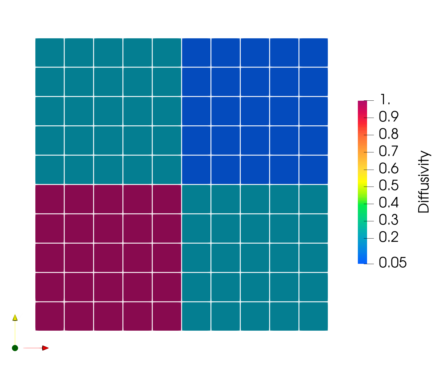
Figure 1: Actual spatially varying thermal conductivity used to produce synthetic temperature data. The optimization simulation is attempting to reproduce this thermal conductivity distribution.
As this is a transient or non-steady problem, the solution at each time step depends on the solution at previous steps. The forward problem is solved as usual in MOOSE, using implicit Euler time stepping. The solution to the thermal problem is obtained for ten steps with a time step of 0.1 seconds. The solution for the temperature field at time s, together with the points where the measured temperatures are taken, is shown in Figure 2.
![Snapshot of the forward simulation at the end of the sixth time step (0.6 s). The spatially varying thermal conductivity in [diff_parameter] is optimized to minimize the difference between the measured and simulated temperature values at the locations shown by the yellow x's.](../../../large_media/optimization/material_transient_solution.png)
Figure 2: Snapshot of the forward simulation at the end of the sixth time step (0.6 s). The spatially varying thermal conductivity in Figure 1 is optimized to minimize the difference between the measured and simulated temperature values at the locations shown by the yellow x's.
The optimization module will initialize the parameters being optimized to zero or the lower_bound for the first optimization iteration. For this problem, an initial thermal conductivity distribution of zero will not be able to find a thermal conductivity distribution that minimizes the temperature misfit. To help the optimization algorithm out, we provide an initial guess for the spatially varying thermal conductivity. In Figure 3, we plot the objective function as we vary the thermal conductivity at the location (0.75, 0.75). The slope of the objective function with respect to variations in the parameter can have implication in the overall convergence of the optimization problem.
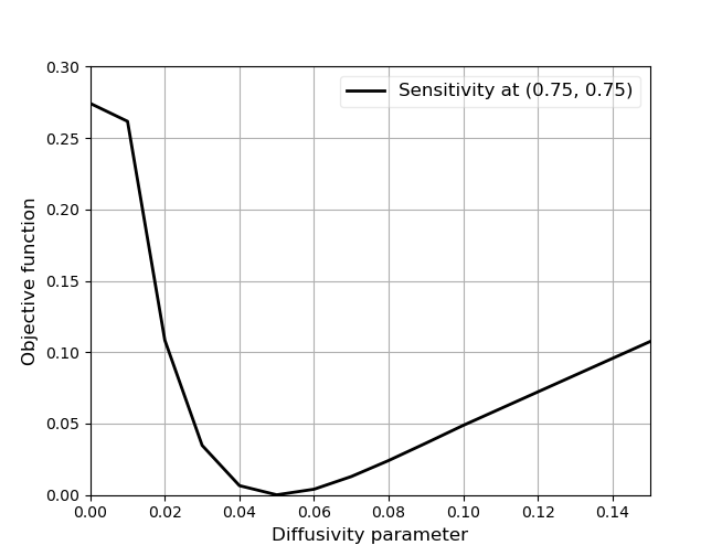
Figure 3: Sensitivity of the objective function when changing the diffusivity parameter at the location (0.75, 0.75) around its optimal value '0.05'.
Problem Input File Setup
This example makes use of the TransientAndAdjoint executioner, which automatically computes the adjoint by transposing the forward problem's Jacobian. This frees the user from having to derive and implement an adjoint input file based on the forward problem kernels. This also solves the forward and adjoint problems in a single sub-application. An alternative method with two child applications corresponding to the forward and adjoint problems is given in Multi-app executioner.
The entire inverse optimization strategy is governed by the OptimizationReporter object. The forward and adjoint problems are set up in the main application input file to be solved as a FullSolveMultiApp type of MultiApps problem. Controllable parameter data is transferred to the to_forward sub-app using the MultiAppReporterTransfer objects. Objective and gradient information is then passed back to the optimization main application using another MultiAppReporterTransfer.
[Optimization<<<{"href": "../../../syntax/Optimization/index.html"}>>>]
[]

[OptimizationReporter<<<{"href": "../../../syntax/OptimizationReporter/index.html"}>>>]
  type = GeneralOptimization
  objective_name = objective_value
  parameter_names = 'D'
  num_values = '4'
  initial_condition = '0.01 0.01 0.01 0.01'
  upper_bounds = '1e2'
  lower_bounds = '1e-3'
[]

[Reporters<<<{"href": "../../../syntax/Reporters/index.html"}>>>]
  [main]
    type = OptimizationData<<<{"description": "Reporter to hold measurement and simulation data for optimization problems", "href": "../../../source/reporters/OptimizationData.html"}>>>

    measurement_file<<<{"description": "CSV file with measurement value and coordinates (value, x, y, z)."}>>> = forward_out_data_0011.csv
    file_xcoord<<<{"description": "x coordinate column name from measurement_file csv being read in."}>>> = measurement_xcoord
    file_ycoord<<<{"description": "y coordinate column name from csv file being read in."}>>> = measurement_ycoord
    file_zcoord<<<{"description": "z coordinate column name from csv file being read in."}>>> = measurement_zcoord
    file_time<<<{"description": "time column name from csv file being read in."}>>> = measurement_time
    file_value<<<{"description": "measurement value column name from csv file being read in."}>>> = simulation_values
  []
[]

[MultiApps<<<{"href": "../../../syntax/MultiApps/index.html"}>>>]
  [forward]
    type = FullSolveMultiApp<<<{"description": "Performs a complete simulation during each execution.", "href": "../../../source/multiapps/FullSolveMultiApp.html"}>>>
    input_files<<<{"description": "The input file for each App.  If this parameter only contains one input file it will be used for all of the Apps.  When using 'positions_from_file' it is also admissable to provide one input_file per file."}>>> = forward_and_adjoint.i
    execute_on<<<{"description": "The list of flag(s) indicating when this object should be executed. For a description of each flag, see https://mooseframework.inl.gov/source/interfaces/SetupInterface.html."}>>> = FORWARD
  []
[]

[Transfers<<<{"href": "../../../syntax/Transfers/index.html"}>>>]
  [to_forward]
    type = MultiAppReporterTransfer<<<{"description": "Transfers reporter data between two applications.", "href": "../../../source/transfers/MultiAppReporterTransfer.html"}>>>
    to_multi_app<<<{"description": "The name of the MultiApp to transfer the data to"}>>> = forward
    from_reporters<<<{"description": "List of the reporter names (object_name/value_name) to transfer the value from."}>>> = 'main/measurement_xcoord
                      main/measurement_ycoord
                      main/measurement_zcoord
                      main/measurement_time
                      main/measurement_values
                      OptimizationReporter/D'
    to_reporters<<<{"description": "List of the reporter names (object_name/value_name) to transfer the value to."}>>> = 'data/measurement_xcoord
                    data/measurement_ycoord
                    data/measurement_zcoord
                    data/measurement_time
                    data/measurement_values
                    diffc_rep/D_vals'
  []
  [from_forward]
    type = MultiAppReporterTransfer<<<{"description": "Transfers reporter data between two applications.", "href": "../../../source/transfers/MultiAppReporterTransfer.html"}>>>
    from_multi_app<<<{"description": "The name of the MultiApp to receive data from"}>>> = forward
    from_reporters<<<{"description": "List of the reporter names (object_name/value_name) to transfer the value from."}>>> = 'data/objective_value
                      adjoint/inner_product'
    to_reporters<<<{"description": "List of the reporter names (object_name/value_name) to transfer the value to."}>>> = 'OptimizationReporter/objective_value
                    OptimizationReporter/grad_D'
  []
[]

[Executioner<<<{"href": "../../../syntax/Executioner/index.html"}>>>]
  type = Optimize
  tao_solver = taobqnls
  petsc_options_iname = '-tao_gatol'
  petsc_options_value = '1e-4'
[]A single input file is used to simulate the physics for the optimization problem. The core of the input file contains the definition of the physics that the user wants to model, as with most of MOOSE's simulations. In this case, a heat diffusion problem with Dirichlet boundary conditions is built. The forward and adjoint problems are run in two separate nonlinear systems, one for the forward problem and another one for the adjoint problem. These nonlinear systems are inputs to an executioner that drives the simulation of both problems, i.e. the TransientAndAdjoint MOOSE object.
[Problem<<<{"href": "../../../syntax/Problem/index.html"}>>>]
  nl_sys_names = 'nl0 adjoint'
  kernel_coverage_check = false
[][Variables<<<{"href": "../../../syntax/Variables/index.html"}>>>]
[u]
initial_condition<<<{"description": "Specifies a constant initial condition for this variable"}>>> = 0
[]
[u_adjoint]
initial_condition<<<{"description": "Specifies a constant initial condition for this variable"}>>> = 0
solver_sys = adjoint
outputs = none
[]
[]For material inversion, the derivative of the objective function with respect to the material parameters needs to be computed. This quantity is problem-dependent.
For this thermal problem, the vector postprocessor ElementOptimizationDiffusionCoefFunctionInnerProduct computes the gradient of the objective with respect to the controllable parameter by computing the inner product between the gradient of the adjoint variable and the gradient of the primal variables and the function computing the derivative of the material property with respect to the controllable parameter.
[VectorPostprocessors<<<{"href": "../../../syntax/VectorPostprocessors/index.html"}>>>]
  [adjoint]
    type = ElementOptimizationDiffusionCoefFunctionInnerProduct<<<{"description": "Compute the gradient for material inversion by taking the inner product of gradients of the forward and adjoint variables with material gradient", "href": "../../../source/vectorpostprocessors/ElementOptimizationDiffusionCoefFunctionInnerProduct.html"}>>>
    variable<<<{"description": "The names of the variables that this VectorPostprocessor operates on"}>>> = u_adjoint
    forward_variable<<<{"description": "Variable from the forward solution"}>>> = u
    function<<<{"description": "Optimization function."}>>> = diffc_fun
    execute_on<<<{"description": "The list of flag(s) indicating when this object should be executed. For a description of each flag, see https://mooseframework.inl.gov/source/interfaces/SetupInterface.html."}>>> = ADJOINT_TIMESTEP_END
    outputs<<<{"description": "Vector of output names where you would like to restrict the output of variables(s) associated with this object"}>>> = none
  []
[]