MOOSE User Short Workshop
Idaho National Laboratory
www.inl.gov
Established in 2005, INL is the lead nuclear energy R&D laboratory for the Department of Energy
"Establish a world-class capability in the modeling and simulation of advanced energy systems..."
INL is the one of the largest employers in Idaho with over 6,000 employees and 500 interns
In 2024 the INL budget was over $2 billion
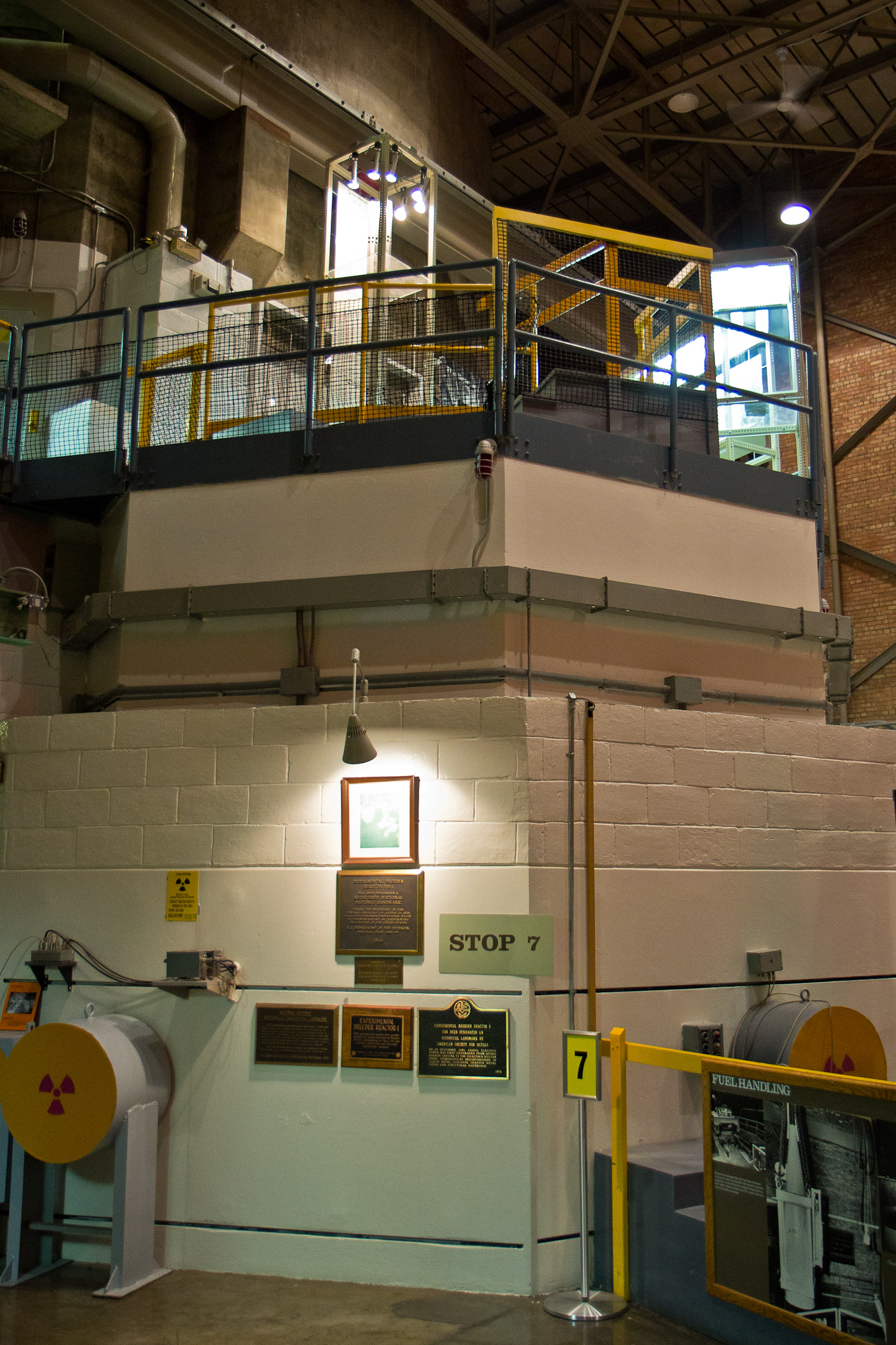
INL is the site where 52 nuclear reactors were designed and constructed, including the first reactor to generate usable amounts of electricity: Experimental Breeder Reactor I (EBR-1)
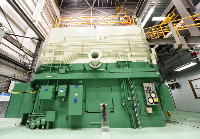
Advanced Test Reactor (ATR)
World's most powerful test reactor (250 MW thermal)
Constructed in 1967
Volume of 1.4 cubic meters, with 43 kg of uranium, and operates at 60C
Transient Reactor Test Facility (TREAT)
TREAT is a test facility specifically designed to evaluate the response of fuels and materials to accident conditions
High-intensity (20 GW), short-duration (80 ms) neutron pulses for severe accident testing
National Reactor Innovation Center (NRIC)
NRIC is composed of two physical test beds to build prototypes of advanced nuclear reactors:
DOME (Demonstration of Microreactor Experiments) in the historic EBR-II facility, a test bed site capable of hosting operational nuclear reactor concepts that produce less than 20MW thermal power.
LOTUS (Laboratory for Operation and Testing in the U.S.) in the historic Zero Power Physics Reactor (ZPPR) Cell, a test bed site capable of hosting operational nuclear reactor concepts that produce less than 500kW thermal power.
NRIC also manages the open-source Virtual Test Bed to demonstrate advanced reactors through modeling and simulation. More information about NRIC can be found at https://nric.inl.gov.
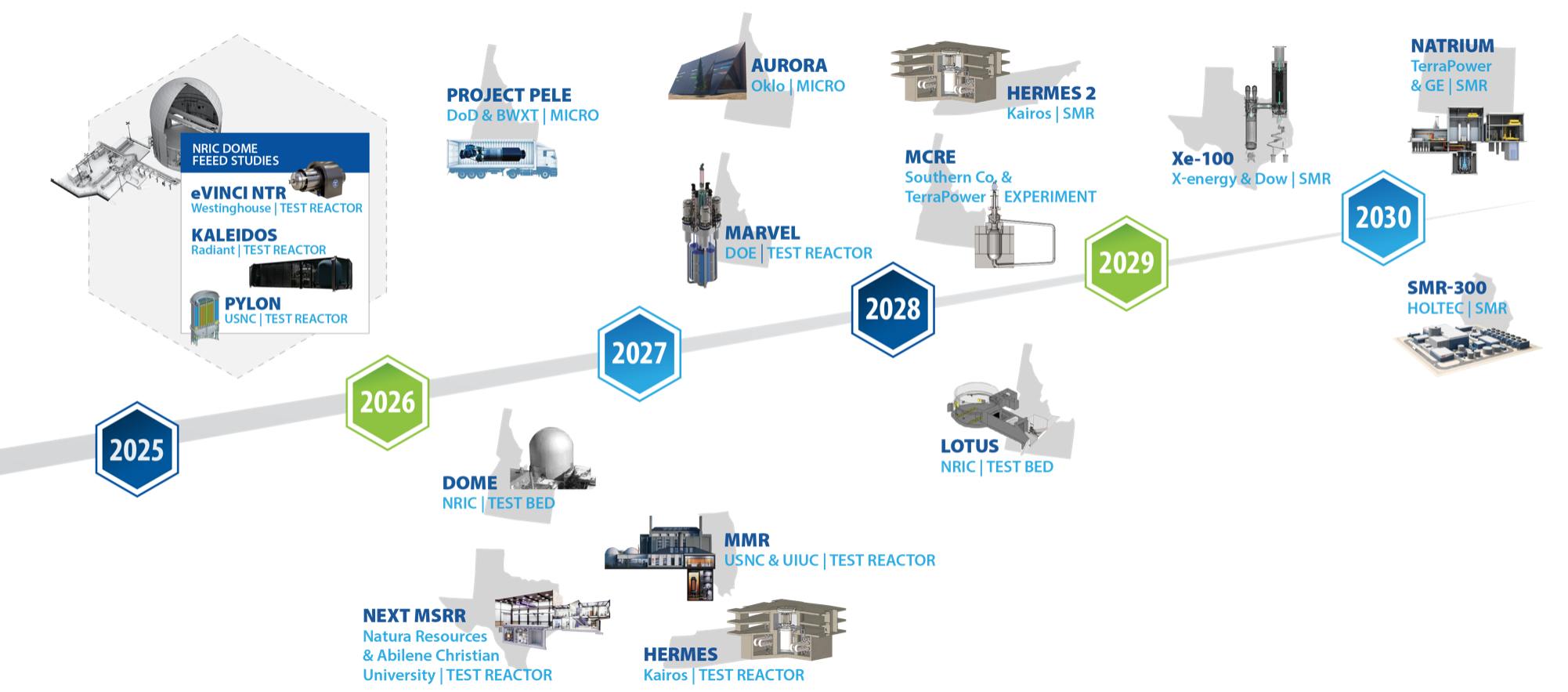
Advanced Reactor Demonstration Timeline
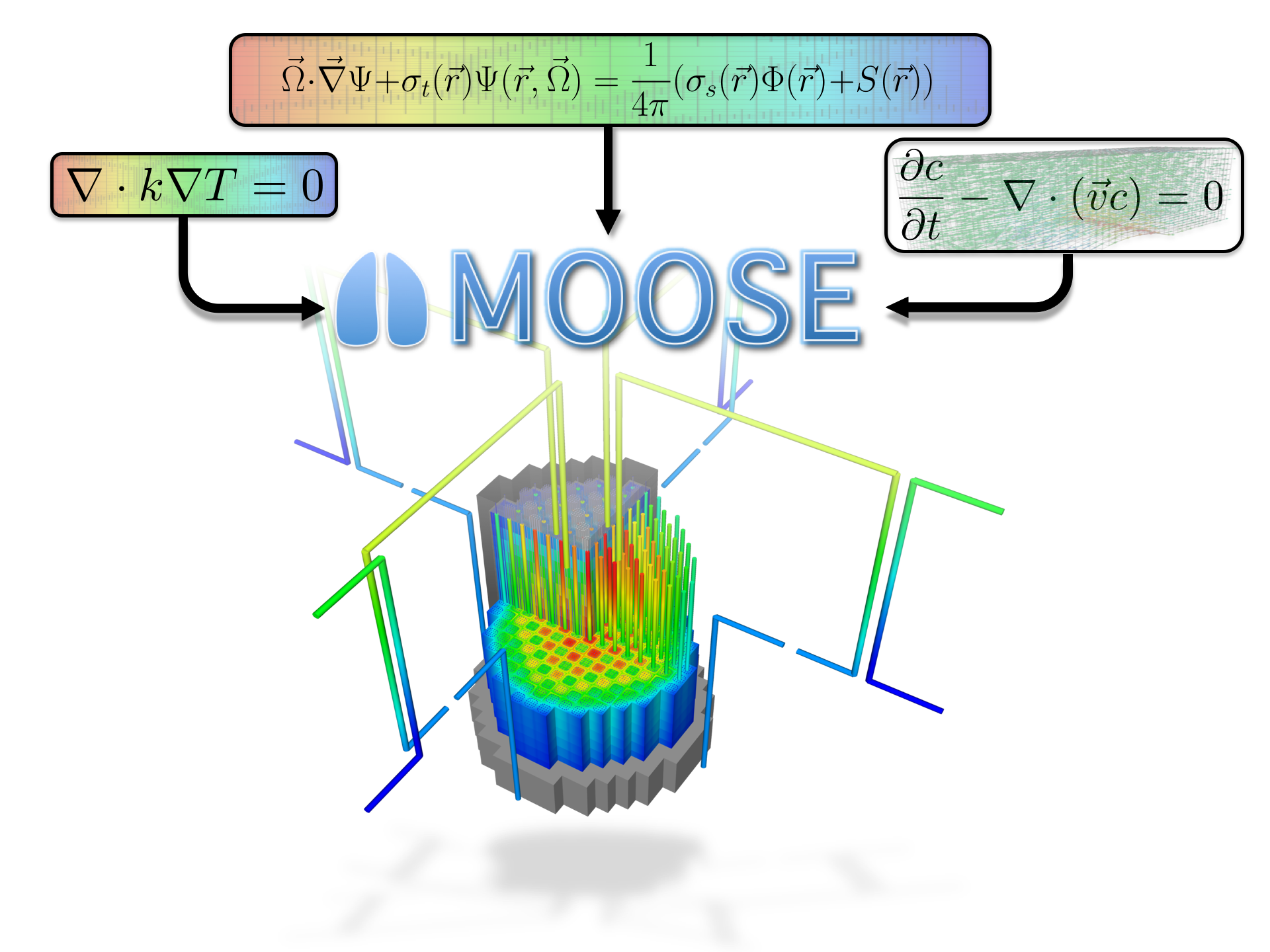
MOOSE
Multi-physics Object Oriented Simulation Environment
mooseframework.inl.gov
History and Purpose
Development started in 2008
Open-sourced in 2014
Designed to solve computational engineering problems and reduce the expense and time required to develop new applications by:
Being easily extended and maintained
Working efficiently on a few and many processors
Providing an object-oriented, extensible system for creating all aspects of a simulation tool
Motivated by multiphysics problems in nuclear engineering, but applications have extended into diverse fields
Core team at Idaho National Laboratory, but with significant contributions from other laboratories, universities, and industry, both domestically and internationally
By The Numbers
250 contributors
58,000 commits
5,000 unique visitors per month
~40 new Discussion participants per week
150M tests per week
General Capabilities
Continuous and Discontinuous Galerkin FEM
Finite Volume
Supports fully coupled or segregated systems, fully implicit and explicit time integration
Automatic differentiation (AD)
Unstructured mesh with FEM shapes
Higher order geometry
Mesh adaptivity (refinement and coarsening)
Massively parallel (MPI and threads)
User code agnostic of dimension, parallelism, shape functions, etc.
Native support for executing multiphysics simulations across applications
GPU support for execution via MFEM and Kokkos
Operating Systems:
macOS (Conda, Docker)
Linux (Apptainer, Conda, Docker)
Windows (Docker, WSL)
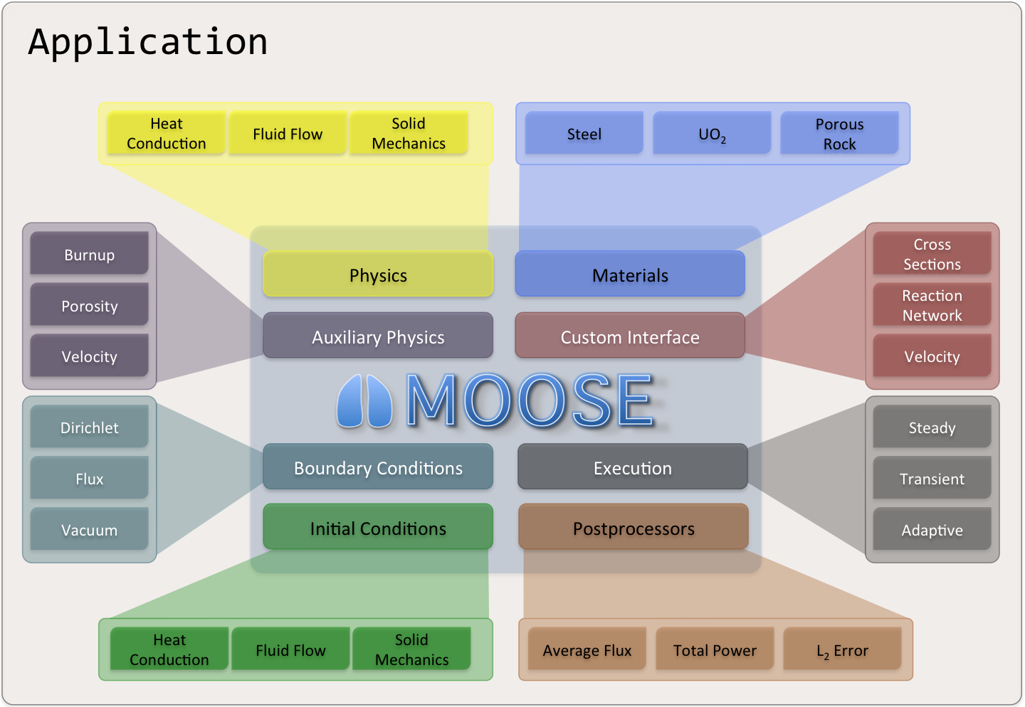
Object-oriented, pluggable system
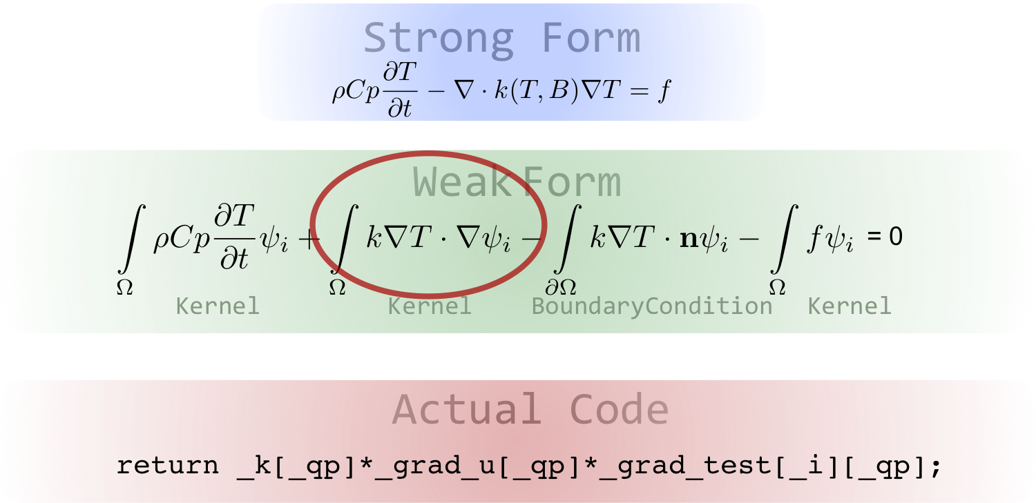
Example Code
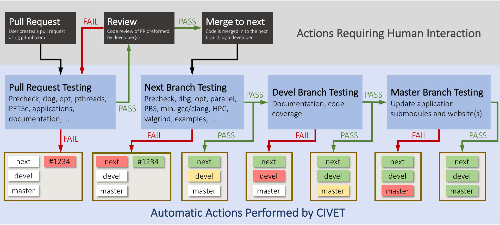
Software Quality
Follows a Nuclear Quality Assurance Level 1 (NQA-1) development process
All changes undergo independent review and must pass regression tests before merge
Includes a test suite and documentation system to allow for agile development while maintaining a NQA-1 process
External contributions are guided through the process by the team, and are very welcome!
Development Process
Community
github.com/idaholab/moose/discussions

License
LGPL 2.1
Does not limit what you can do with your application
Can license/sell your application as closed source
Modifications to the library itself (or the modules) are open source
New contributions are automatically LGPL 2.1
MOOSE Modules and Applications
MOOSE Modules
MOOSE has numerous optional modules:
Physics
Chemical Reactions
Contact
Electromagnetics
Fluid Structure Interaction (FSI)
Geochemistry
Heat Transfer
Level Set
Navier Stokes
Peridynamics
Phase Field
Porous Flow
Solid Mechanics
Subchannel
Thermal Hydraulics
Numerics
External PETSc Solver
Function Expansion Tools
Optimization
Ray Tracing
rDG
Stochastic Tools
XFEM
Physics support
Fluid Properties
Solid Properties
Reactor
MOOSE Ecosystem
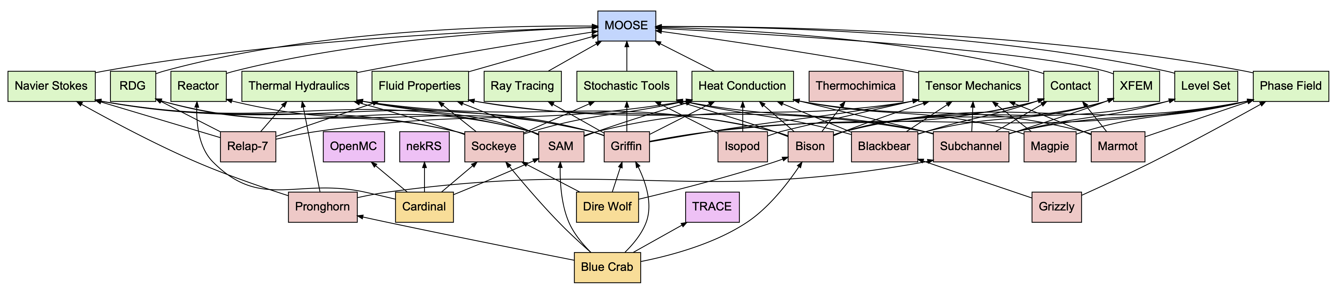
Open-Source Applications
Some open-source MOOSE applications:
NCRC Applications
The Nuclear Computational Resource Center (NCRC) licenses several MOOSE applications:
| Code | Description |
|---|---|
| Bison | Fuel performance, thermomechanics |
| BlueCRAB | Multiphysics (Griffin, Bison, Pronghorn, SAM, TRACE, Sockeye) |
| DireWolf | Microreactor multiphysics (Griffin, Bison, Sockeye) |
| Griffin | Deterministic radiation transport |
| Grizzly | Component aging |
| Pronghorn | Coarse-mesh thermal hydraulics |
| SAM | Advanced reactor systems analysis |
| Sabertooth | Multiphysics (Griffin, Bison, RELAP-7) |
| Sockeye | Heat pipe analysis |
Apply for access: NCRC
Multiphysics Simulation
Historical Multiphysics Simulation
Predictive multiphysics capability involved best-estimate calculations
Best estimates: data and correlation driven, many approximations
Necessitated experimental data for each design
Physics performed independently
Was a "siloed" task; handoffs of data/results from person to person
While individual codes were computationally efficient and well validated, coupling them was neither efficient nor well validated
Used many approximations for evaluations of safety parameters
Pin-power reconstruction, gap conductance, spacer grid models
Modern Multiphysics Simulation
Direct, physics-based models of all components
Reduces approximations as needed
Can be computationally expensive
Can employ tighter and more consistent coupling
Length and time scales of physics can be vastly different
What does this change for the analyst?
Not as well validated:
Experiments prohibitively expensive
Very large design space
Modularity is Key
Data should be accessed through strict interfaces with code having separation of responsibilities
Allows for "decoupling" of code
Leads to more reuse and less bugs
Challenging for FEM
Shape functions, degrees of freedom, meshing, quadrature points, material properties, analytic functions, global integrals, data transfer, ...
The complexity makes computational science codes brittle and hard to reuse
A consistent set of "systems" are needed to carry out common actions, these systems should be separated by interfaces
Finite-Element Reactor Fuel Simulation
MOOSE Coupling Strategies
Coupling strategies:
Full coupling: Solve all physics in a single (linear or nonlinear) system
Loose coupling: Solve each physics sequentially
Tight coupling: Solve each physics sequentially and iterate
Segregated (loose/tight) coupling achieved using
MultiAppsPhysics coupled via in-memory transfer of fields and scalars
Coupling specified in the input file (no code needed)
No universally superior coupling strategy; correct choice depends on problem
Provides a standardized interface for an analyst to produce a coupled model
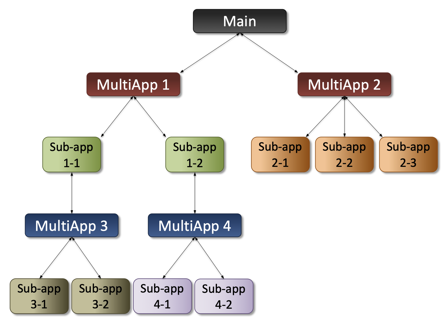
MOOSE MultiApp Hierarchy Example
Tutorial Steps
Step 1: Input and Meshing
MOOSE Input
An input file defines a MOOSE simulation and follows a standardized syntax, the "hierarchical input text" (HIT) format.
A basic MOOSE input file typically has six "blocks":
[Mesh]: Define the geometry of the domain[Variables]: Define the unknown(s) of the problem[Kernels]: Define the equation(s) to solve[BCs]: Define the boundary condition(s) of the problem[Executioner]: Define how the problem will be solved[Outputs]: Define how the solution will be returned
There are caveats to the above and many other blocks exist. Shortcut syntax can also be created to simplify input.
A listing of all syntax can be found here.
The Moose Language Support VSCode extension adds diagnostics and autocompletion to input in VSCode.
Introduction to Input
We will work through the process of mesh generation as an introduction to building MOOSE input.
The first step will be the generation of a mesh that is uniform two-dimensional grid using the GeneratedMeshGenerator.
Basic Mesh Input
[Mesh<<<{"href": "../syntax/Mesh/index.html"}>>>]
  [gmg]
    type = GeneratedMeshGenerator<<<{"description": "Create a line, square, or cube mesh with uniformly spaced or biased elements.", "href": "../source/meshgenerators/GeneratedMeshGenerator.html"}>>>
    dim<<<{"description": "The dimension of the mesh to be generated"}>>> = 2
    nx<<<{"description": "Number of elements in the X direction"}>>> = 10
    ny<<<{"description": "Number of elements in the Y direction"}>>> = 10
  []
[]The above defines a GeneratedMeshGenerator named gmg with the parameters:
dim: sets the dimension tonx: which builds elements in the -directionny: which builds elements in the -direction
Run: Basic Mesh Input
$ cd moose/step1_input_and_meshing
$ moose-opt -i basic.i --mesh-only
The argument
-ispecifies which input file to runThe
--mesh-onlyargument forces only mesh generation and output in Exodus formatWithout arguments to
--mesh-only, the mesh will be output as Exodus in the same folder as the input with the name<input_file>_in.e, i.e.,basic_in.eIf an argument is provided to
--mesh-only, that argument will be used as the output path for the generated mesh
This output format, Exodus, is commonly inspected using Paraview
Result: Basic Mesh Input
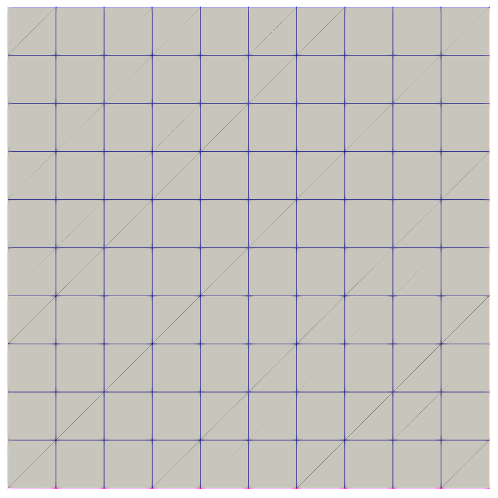
From basic_in.e in Paraview
MeshGenerator System
The previous example utilized the MOOSE MeshGenerator system:
Enables the programmatic construction of a mesh
Generation can be chained together through dependencies so that complex meshes may be built up from a series of simple processes
Several built-in generators exist but you can develop your own MeshGenerators
Built-in examples: building grids and concentric circles; triangulation and tetrahedralization; extrusion; renaming and merging of blocks and sidesets; stitching; scaling, translating, and rotating; image conversion
Supports distributed mesh generation and modification
Enables the addition of "metadata" to meshes
Particularly useful in neutronics for storing things like depletion zones
All of our examples that follow (including the Cardinal tutorial) will utilize the MeshGenerator system. Of significant note is the Reactor module, which supports the systematic mesh generation of common reactor types.
Loading Meshes From File
Meshes can also be loaded from file, of which we support a variety of formats like Exodus, GMSH, Nemesis, Tecplot, VTK, etc
[Mesh]
  [from_file]
    type = FileMeshGenerator
    file = foo.e
  []
[]
Other Input Syntax
# Include the input at file.i here
!include file.i

value = true       # boolean
value = '1 2 3 4'  # vector -> [1, 2, 3, 4]
value = '1 2; 3 4' # vector-of-vectors -> [[1, 2], [3, 4]]

# Equivalent to [Mesh][gmg]
[Mesh/gmg]
  type = GeneratedMeshGenerator
  ...
[]

# Reference another value
value = 1.0
another_value = ${value}

# Perform basic arithmetic on another parameter (raidus = 0.5)
diameter = 1.0
radius = ${fparse diameter/2}
Concentric Circle Mesh
The grid we first generated isn't particularly interesting.
Let's generate a mesh that represents represents a fuel pin surrounded by water in a square lattice using the ConcentricCircleMeshGenerator with the following dimensions:
| Quantity | Value |
|---|---|
| Hole radius | cm |
| Pellet radius | cm |
| Clad radius | cm |
| Pitch | cm |
We will also apply a special treatment at the clad-fluid interface to support a thermal-hydraulics solve with a boundary layer.
Input: Concentric Circle Mesh
hole_radius = 0.08e-2     # [m]
pellet_radius = 0.26e-2   # [m]
clad_radius = 0.3e-2      # [m]
water_radius = 0.3475e-2  # [m]

boundary_layer_frac = 0.1
boundary_layer_radius = ${fparse ((water_radius - clad_radius) * boundary_layer_frac + clad_radius)}

[Mesh<<<{"href": "../syntax/Mesh/index.html"}>>>]
  [concentric_circle]
    type = ConcentricCircleMeshGenerator<<<{"description": "This ConcentricCircleMeshGenerator source code is to generate concentric circle meshes.", "href": "../source/meshgenerators/ConcentricCircleMeshGenerator.html"}>>>
    num_sectors<<<{"description": "num_sectors % 2 = 0, num_sectors > 0Number of azimuthal sectors in each quadrant'num_sectors' must be an even number."}>>> = 12
    radii<<<{"description": "Radii of major concentric circles"}>>> = '${hole_radius} ${pellet_radius} ${clad_radius} ${boundary_layer_radius}'
    has_outer_square<<<{"description": "It determines if meshes for a outer square are added to concentric circle meshes."}>>> = true
    preserve_volumes<<<{"description": "Volume of concentric circles can be preserved using this function."}>>> = false
    rings<<<{"description": "Number of rings in each circle or in the enclosing square"}>>> = '1 3 1 1 3'
    pitch<<<{"description": "The enclosing square can be added to the completed concentric circle mesh.Elements are quad meshes."}>>> = ${fparse water_radius * 2}
  []
[]Run: Concentric Circle Mesh
$ moose-opt -i concentric_circle.i --mesh-only
 Mesh Information:
  elem_dimensions()={2}
  elem_default_orders()={FIRST}
  supported_nodal_order()=1
  spatial_dimension()=2
  n_nodes()=729
    n_local_nodes()=729
  n_elem()=688
    n_local_elem()=688
    n_active_elem()=688
  n_subdomains()=5
  n_elemsets()=0
  n_partitions()=1
  n_processors()=1
  n_threads()=1
  processor_id()=0
  is_prepared()=true
  is_replicated()=true

 Mesh Bounding Box:
  Minimum: (x,y,z)=(-0.003475, -0.003475,        0)
  Maximum: (x,y,z)=(0.003475, 0.003475,        0)
  Delta:   (x,y,z)=( 0.00695,  0.00695,        0)

 Mesh Element Type(s):
  QUAD4

 Mesh Nodesets:
  Nodeset 1, 21 nodes
   Bounding box minimum: (x,y,z)=(-0.003475, -0.003475,        0)
   Bounding box maximum: (x,y,z)=(-0.003475, 0.003475,        0)
   Bounding box delta: (x,y,z)=(4.33681e-19,  0.00695,        0)
  Nodeset 2, 21 nodes
   Bounding box minimum: (x,y,z)=(-0.003475, -0.003475,        0)
   Bounding box maximum: (x,y,z)=(0.003475, -0.003475,        0)
   Bounding box delta: (x,y,z)=( 0.00695, 8.67362e-19,        0)
  Nodeset 3, 21 nodes
   Bounding box minimum: (x,y,z)=(0.003475, -0.003475,        0)
   Bounding box maximum: (x,y,z)=(0.003475, 0.003475,        0)
   Bounding box delta: (x,y,z)=(4.33681e-19,  0.00695,        0)
  Nodeset 4, 21 nodes
   Bounding box minimum: (x,y,z)=(-0.003475, 0.003475,        0)
   Bounding box maximum: (x,y,z)=(0.003475, 0.003475,        0)
   Bounding box delta: (x,y,z)=( 0.00695,        0,        0)

 Mesh Sidesets:
  Sideset 1 (left), 20 sides (EDGE2), 20 elems (QUAD4), 21 nodes
   Side volume: 0.00695
   Bounding box minimum: (x,y,z)=(-0.003475, -0.003475,        0)
   Bounding box maximum: (x,y,z)=(-0.003475, 0.003475,        0)
   Bounding box delta: (x,y,z)=(4.33681e-19,  0.00695,        0)
  Sideset 2 (bottom), 20 sides (EDGE2), 20 elems (QUAD4), 21 nodes
   Side volume: 0.00695
   Bounding box minimum: (x,y,z)=(-0.003475, -0.003475,        0)
   Bounding box maximum: (x,y,z)=(0.003475, -0.003475,        0)
   Bounding box delta: (x,y,z)=( 0.00695, 8.67362e-19,        0)
  Sideset 3 (right), 20 sides (EDGE2), 20 elems (QUAD4), 21 nodes
   Side volume: 0.00695
   Bounding box minimum: (x,y,z)=(0.003475, -0.003475,        0)
   Bounding box maximum: (x,y,z)=(0.003475, 0.003475,        0)
   Bounding box delta: (x,y,z)=(4.33681e-19,  0.00695,        0)
  Sideset 4 (top), 20 sides (EDGE2), 20 elems (QUAD4), 21 nodes
   Side volume: 0.00695
   Bounding box minimum: (x,y,z)=(-0.003475, 0.003475,        0)
   Bounding box maximum: (x,y,z)=(0.003475, 0.003475,        0)
   Bounding box delta: (x,y,z)=( 0.00695,        0,        0)

 Mesh Edgesets:
  None

 Mesh Subdomains:
  Subdomain 1: 192 elems (QUAD4, 192 active), 217 active nodes
   Volume: 2.00488e-06
   Bounding box minimum: (x,y,z)=( -0.0008,  -0.0008,        0)
   Bounding box maximum: (x,y,z)=(  0.0008,   0.0008,        0)
   Bounding box delta: (x,y,z)=(  0.0016,   0.0016,        0)
  Subdomain 2: 144 elems (QUAD4, 144 active), 192 active nodes
   Volume: 1.91717e-05
   Bounding box minimum: (x,y,z)=( -0.0026,  -0.0026,        0)
   Bounding box maximum: (x,y,z)=(  0.0026,   0.0026,        0)
   Bounding box delta: (x,y,z)=(  0.0052,   0.0052,        0)
  Subdomain 3: 48 elems (QUAD4, 48 active), 96 active nodes
   Volume: 7.01709e-06
   Bounding box minimum: (x,y,z)=(  -0.003,   -0.003,        0)
   Bounding box maximum: (x,y,z)=(   0.003,    0.003,        0)
   Bounding box delta: (x,y,z)=(   0.006,    0.006,        0)
  Subdomain 4: 48 elems (QUAD4, 48 active), 96 active nodes
   Volume: 8.99867e-07
   Bounding box minimum: (x,y,z)=(-0.0030475, -0.0030475,        0)
   Bounding box maximum: (x,y,z)=(0.0030475, 0.0030475,        0)
   Bounding box delta: (x,y,z)=(0.006095, 0.006095,        0)
  Subdomain 5: 256 elems (QUAD4, 256 active), 320 active nodes
   Volume: 1.9209e-05
   Bounding box minimum: (x,y,z)=(-0.003475, -0.003475,        0)
   Bounding box maximum: (x,y,z)=(0.003475, 0.003475,        0)
   Bounding box delta: (x,y,z)=( 0.00695,  0.00695,        0)
  Global mesh volume = 4.83025e-05
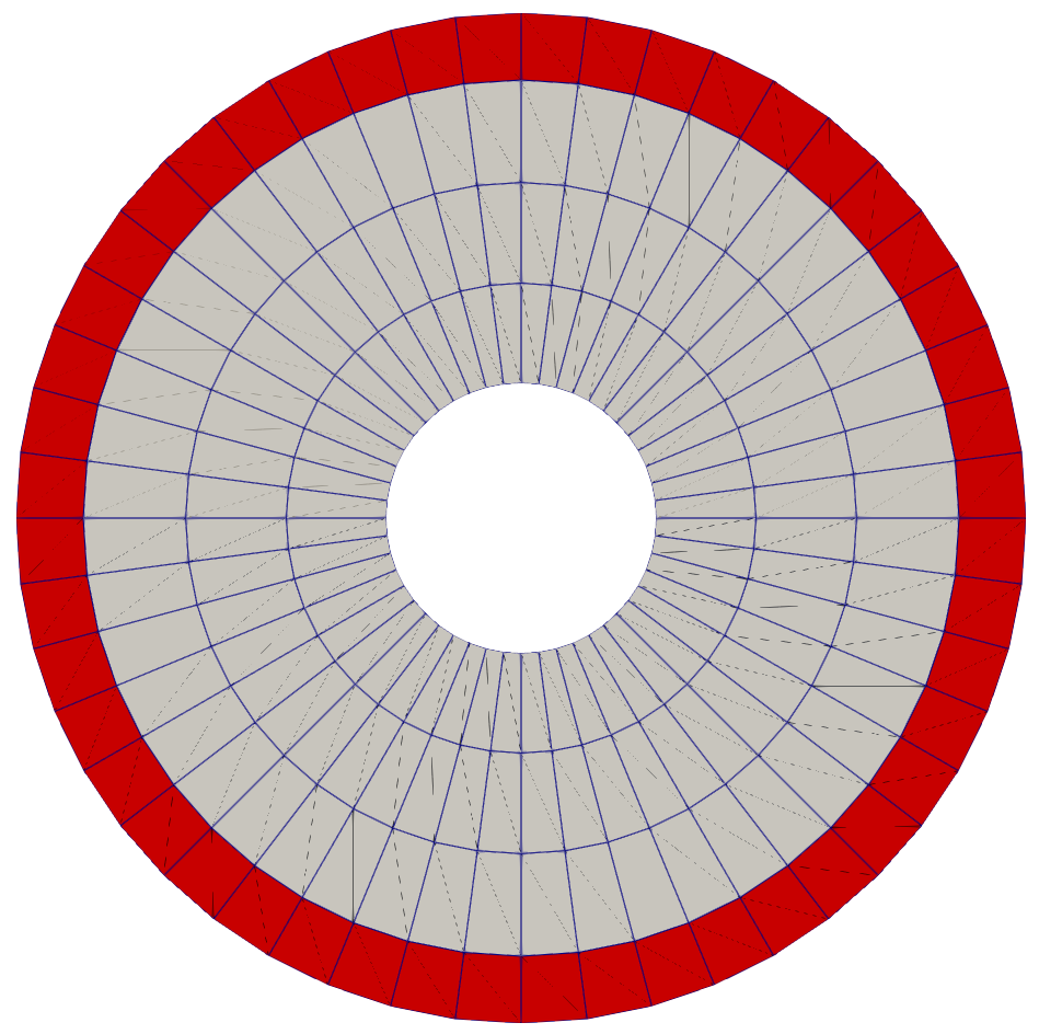
Result: Concentric Circle Mesh Input
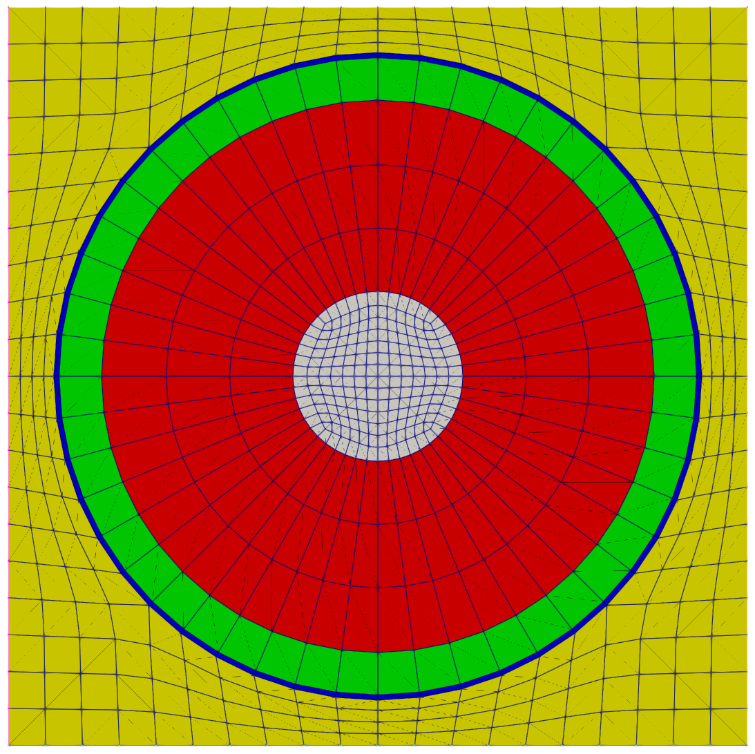
This mesh in concentric_circle_in.e has five blocks (also called subdomains):
: Inner hole (grey)
: Fuel (red)
: Cladding (green)
: Fluid boundary layer (blue)
: Remaining fluid (yellow)
Separating Meshes
Later in this tutorial, we will be treating the fuel pin and the surrounding fluid independently. Thus, we will now take the mesh that we just generated and separate it into two components: one for the fuel pin and one for the fluid.
This task reveals a capability of MeshGenerators – they can be combined together. Some MeshGenerators generate meshes, some modify meshes, and some do both. Oftentimes a generator will have an input parameter called input, which is used as the name of another MeshGenerator to be used as input to modify.
For the tasks that follow, we will utilize the:
BlockDeletionGenerator: Removes blocks from a meshRenameBlockGenerator: Renames and optionally merges blocks on a meshRenameBoundaryGenerator: Renames and optionally merges boundaries on a mesh
Fuel Mesh
Remove the hole (assume no net heat transfer across the hole) using the
BlockDeletionGeneratorRemove the water elements using the
BlockDeletionGeneratorName the blocks that contain the fuel and cladding using the
RenameBlockGenerator
Input: Fuel Mesh
# Include Mesh/concentric_circle, which builds the
# full concentric circle mesh
!include concentric_circle.i

[Mesh]
  # Remove block 1 (hole) and define a boundary
  # "inner" on the interface (the inside)
  [remove_hole]
    type = BlockDeletionGenerator
    input = concentric_circle
    block = 1
    new_boundary = inner
  []

  # Remove block 4 (water boundary layer) and
  # block 5 (water bulk) and define a boundary
  # "water_solid_interface" on the interface
  # (the outside)
  [remove_water]
    type = BlockDeletionGenerator
    input = remove_hole
    block = '4 5'
    new_boundary = water_solid_interface
  []

  # Rename the remaining blocks (2: fuel, 3: clad)
  [rename_blocks]
    type = RenameBlockGenerator
    input = remove_water
    old_block = '2 3'
    new_block = 'fuel clad'
  []
[]
Run: Fuel Mesh
$ moose-opt -i fuel_pin.i --mesh-only
 Mesh Information:
  elem_dimensions()={2}
  elem_default_orders()={FIRST}
  supported_nodal_order()=1
  spatial_dimension()=2
  n_nodes()=240
    n_local_nodes()=240
  n_elem()=192
    n_local_elem()=192
    n_active_elem()=192
  n_subdomains()=2
  n_elemsets()=0
  n_partitions()=1
  n_processors()=1
  n_threads()=1
  processor_id()=0
  is_prepared()=true
  is_replicated()=true

 Mesh Bounding Box:
  Minimum: (x,y,z)=(  -0.003,   -0.003,        0)
  Maximum: (x,y,z)=(   0.003,    0.003,        0)
  Delta:   (x,y,z)=(   0.006,    0.006,        0)

 Mesh Element Type(s):
  QUAD4

 Mesh Nodesets:
  Nodeset 5, 48 nodes
   Bounding box minimum: (x,y,z)=( -0.0008,  -0.0008,        0)
   Bounding box maximum: (x,y,z)=(  0.0008,   0.0008,        0)
   Bounding box delta: (x,y,z)=(  0.0016,   0.0016,        0)
  Nodeset 6, 48 nodes
   Bounding box minimum: (x,y,z)=(  -0.003,   -0.003,        0)
   Bounding box maximum: (x,y,z)=(   0.003,    0.003,        0)
   Bounding box delta: (x,y,z)=(   0.006,    0.006,        0)

 Mesh Sidesets:
  Sideset 5 (inner), 48 sides (EDGE2), 48 elems (QUAD4), 48 nodes
   Side volume: 0.00502296
   Bounding box minimum: (x,y,z)=( -0.0008,  -0.0008,        0)
   Bounding box maximum: (x,y,z)=(  0.0008,   0.0008,        0)
   Bounding box delta: (x,y,z)=(  0.0016,   0.0016,        0)
  Sideset 6 (water_solid_interface), 48 sides (EDGE2), 48 elems (QUAD4), 48 nodes
   Side volume: 0.0188361
   Bounding box minimum: (x,y,z)=(  -0.003,   -0.003,        0)
   Bounding box maximum: (x,y,z)=(   0.003,    0.003,        0)
   Bounding box delta: (x,y,z)=(   0.006,    0.006,        0)

 Mesh Edgesets:
  None

 Mesh Subdomains:
  Subdomain 2 (fuel): 144 elems (QUAD4, 144 active), 192 active nodes
   Volume: 1.91717e-05
   Bounding box minimum: (x,y,z)=( -0.0026,  -0.0026,        0)
   Bounding box maximum: (x,y,z)=(  0.0026,   0.0026,        0)
   Bounding box delta: (x,y,z)=(  0.0052,   0.0052,        0)
  Subdomain 3 (clad): 48 elems (QUAD4, 48 active), 96 active nodes
   Volume: 7.01709e-06
   Bounding box minimum: (x,y,z)=(  -0.003,   -0.003,        0)
   Bounding box maximum: (x,y,z)=(   0.003,    0.003,        0)
   Bounding box delta: (x,y,z)=(   0.006,    0.006,        0)
  Global mesh volume = 2.61888e-05
Result: Fuel Mesh
From fuel_pin_in.e: The grey elements represent the fuel (block fuel), and the red elements represent the cladding (block clad). There is a sideset on the outer boundary with name water_solid_interface and sideset on the inner boundary with the name inner.
Fluid Mesh
Remove the fuel pin elements using the
BlockDeletionGeneratorMerge the water boundary layer and remaining water blocks into a single block named
waterusing theRenameBlockGeneratorRename and merge the outer boundaries into a single boundary
outerusing theRenameBoundaryGenerator
Input: Fluid Mesh
# Include Mesh/concentric_circle, which builds the
# full concentric circle mesh
!include concentric_circle.i

[Mesh]
  # Remove block 1 (hole), 2 (fuel), 3 (clad)
  # and define a boundary "water_solid_interface"
  # on the interface (the inside)
  [remove_fuel_pin]
    type = BlockDeletionGenerator
    input = concentric_circle
    block = '1 2 3'
    new_boundary = water_solid_interface
  []

  # Merge the remaining blocks (4 - water boundary layer,
  # 5 - water bulk) into a single block "water"
  [rename_blocks]
    type = RenameBlockGenerator
    input = remove_fuel_pin
    old_block = '4 5'
    new_block = 'water water'
  []

  # Rename and merge the outer boundaries created by
  # the ConcentricCircleMeshGenerator (top, right,
  # bottom, left) into a single boundary (water)
  [merge_outer]
    type = RenameBoundaryGenerator
    input = rename_blocks
    old_boundary = 'top right bottom left'
    new_boundary = 'outer outer outer outer'
  []
[]
Run: Fluid Mesh
$ moose-opt -i fluid.i --mesh-only
 Mesh Information:
  elem_dimensions()={2}
  elem_default_orders()={FIRST}
  supported_nodal_order()=1
  spatial_dimension()=2
  n_nodes()=368
    n_local_nodes()=368
  n_elem()=304
    n_local_elem()=304
    n_active_elem()=304
  n_subdomains()=1
  n_elemsets()=0
  n_partitions()=1
  n_processors()=1
  n_threads()=1
  processor_id()=0
  is_prepared()=true
  is_replicated()=true

 Mesh Bounding Box:
  Minimum: (x,y,z)=(-0.003475, -0.003475,        0)
  Maximum: (x,y,z)=(0.003475, 0.003475,        0)
  Delta:   (x,y,z)=( 0.00695,  0.00695,        0)

 Mesh Element Type(s):
  QUAD4

 Mesh Nodesets:
  Nodeset 4, 80 nodes
   Bounding box minimum: (x,y,z)=(-0.003475, -0.003475,        0)
   Bounding box maximum: (x,y,z)=(0.003475, 0.003475,        0)
   Bounding box delta: (x,y,z)=( 0.00695,  0.00695,        0)
  Nodeset 5, 48 nodes
   Bounding box minimum: (x,y,z)=(  -0.003,   -0.003,        0)
   Bounding box maximum: (x,y,z)=(   0.003,    0.003,        0)
   Bounding box delta: (x,y,z)=(   0.006,    0.006,        0)

 Mesh Sidesets:
  Sideset 4 (outer), 80 sides (EDGE2), 76 elems (QUAD4), 80 nodes
   Side volume: 0.0278
   Bounding box minimum: (x,y,z)=(-0.003475, -0.003475,        0)
   Bounding box maximum: (x,y,z)=(0.003475, 0.003475,        0)
   Bounding box delta: (x,y,z)=( 0.00695,  0.00695,        0)
  Sideset 5 (water_solid_interface), 48 sides (EDGE2), 48 elems (QUAD4), 48 nodes
   Side volume: 0.0188361
   Bounding box minimum: (x,y,z)=(  -0.003,   -0.003,        0)
   Bounding box maximum: (x,y,z)=(   0.003,    0.003,        0)
   Bounding box delta: (x,y,z)=(   0.006,    0.006,        0)

 Mesh Edgesets:
  None

 Mesh Subdomains:
  Subdomain 4 (water): 304 elems (QUAD4, 304 active), 368 active nodes
   Volume: 2.01088e-05
   Bounding box minimum: (x,y,z)=(-0.003475, -0.003475,        0)
   Bounding box maximum: (x,y,z)=(0.003475, 0.003475,        0)
   Bounding box delta: (x,y,z)=( 0.00695,  0.00695,        0)
  Global mesh volume = 2.01088e-05
Result: Fluid Mesh
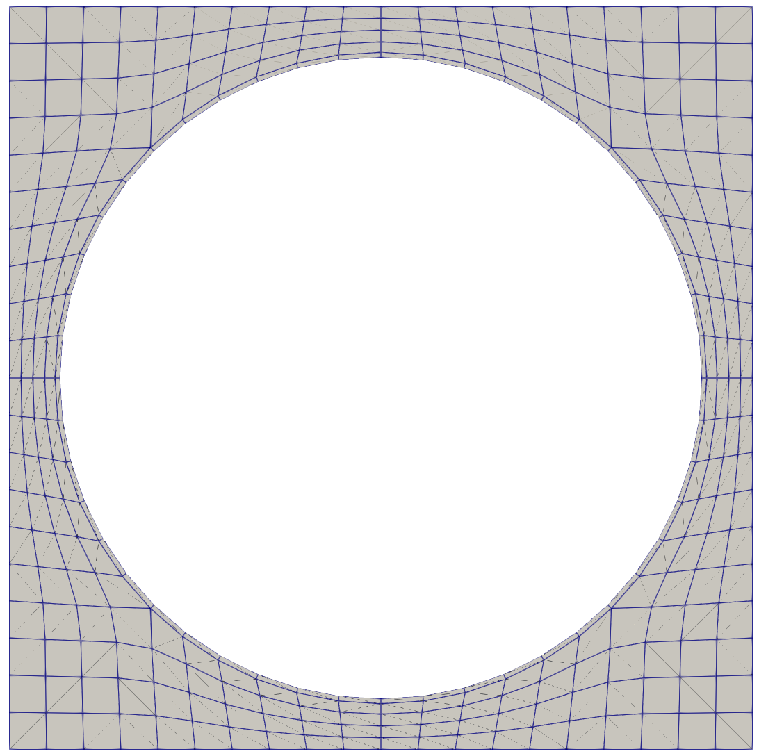
From fluid_in.e: The grey elements represent the water (block water). There is a sideset on the inner boundary with the name water_solid_interface and a sideset on the outer boundary with the name outer.
Reusing the Meshes
We can then load these meshes in later inputs with:
[Mesh/fuel_pin]
  type = FileMeshGenerator
  file = ../step1_input_and_meshing/fuel_pin_in.e
[]
[Mesh/fluid]
  type = FileMeshGenerator
  file = ../step1_input_and_meshing/fluid_in.e
[]
Step 2: Diffusion
Diffusion Problem
Let's solve a diffusion problem on our pin mesh to introduce the solving of a basic finite element problem.
Consider the steady-state diffusion equation on the domain (our pin cell mesh, ../step1_input_and_meshing/fuel_pin_in.e): find such that
where on the interior boundary (inner) and on the exterior boundary (water_solid_interface).
Multiplying by the test function and integrating by parts gives the weak form of this equation, where is our numerical solution:
Required MOOSE Systems
We will utilize the following systems in MOOSE in addition to [Mesh] in our input:
[Variables]: Define the unknown(s) of the problemThe variable
[Kernels]: Define the equation(s) to solveThe diffusion operator
[BCs]: Define the boundary condition(s) of the problemDirichlet boundary conditions on the interior and exterior
[Executioner]: Define how the problem will be solvedA steady state problem
[Outputs]: Define how the solution will be returnedExodus output for field visualization
Variable Definition
Define the variable :
[Variables<<<{"href": "../syntax/Variables/index.html"}>>>]
  [u]
  []
[]Variables can be thought of as the equation(s) you are trying to solve.
The default parameters designate first-order linear Lagrange shape functions, thus without any additional parameters we end up with these shape functions.
Kernel Definition
Define a Diffusion kernel on the variable u:
[Kernels<<<{"href": "../syntax/Kernels/index.html"}>>>]
  [diffusion]
    type = Diffusion<<<{"description": "The Laplacian operator ($-\\nabla \\cdot \\nabla u$), with the weak form of $(\\nabla \\phi_i, \\nabla u_h)$.", "href": "../source/kernels/Diffusion.html"}>>>
    variable<<<{"description": "The name of the variable that this residual object operates on"}>>> = u
  []
[]A Kernel represents an object that contributes to the residual and the Jacobian matrix. Multiple can be used and they can also be coupled to one another to add nonlinearity.
Kernels can be "block restricted" (applied to a subset of the physical mesh) via the block parameter.
Boundary Condition Definition
Define two DirichletBC boundary conditions on the variable u; one on the boundary inner with a value of 0 and one on the boundary water_solid_interface with a value of 1:
[BCs<<<{"href": "../syntax/BCs/index.html"}>>>]
  [inner_dirichlet]
    type = DirichletBC<<<{"description": "Imposes the essential boundary condition $u=g$, where $g$ is a constant, controllable value.", "href": "../source/bcs/DirichletBC.html"}>>>
    variable<<<{"description": "The name of the variable that this residual object operates on"}>>> = u
    boundary<<<{"description": "The list of boundary IDs from the mesh where this object applies"}>>> = inner
    value<<<{"description": "Value of the BC"}>>> = 0
  []
  [outer_dirichlet]
    type = DirichletBC<<<{"description": "Imposes the essential boundary condition $u=g$, where $g$ is a constant, controllable value.", "href": "../source/bcs/DirichletBC.html"}>>>
    variable<<<{"description": "The name of the variable that this residual object operates on"}>>> = u
    boundary<<<{"description": "The list of boundary IDs from the mesh where this object applies"}>>> = water_solid_interface
    value<<<{"description": "Value of the BC"}>>> = 1
  []
[]Executioner Definition
Define a Steady executioner:
[Executioner<<<{"href": "../syntax/Executioner/index.html"}>>>]
  type = Steady
[]The other common executioner is the Transient executioner, which enables transient simulation.
Output Definition
Use the shorthand Outputs/exodus syntax for enabling Exodus output:
[Outputs<<<{"href": "../syntax/Outputs/index.html"}>>>]
  exodus<<<{"description": "Output the results using the default settings for Exodus output."}>>> = true
[]The shorthand syntax effectively creates a Exodus output where the output files are created with the name <input_file_name>_out.e (in our case, diffusion_out.e)
Other common shorthand syntax are Outputs/csv for CSV output and Outputs/nemesis for Nemesis (distributed Exodus) field output.
Input: Diffusion Problem
[Mesh<<<{"href": "../syntax/Mesh/index.html"}>>>/fuel_pin]
  type = FileMeshGenerator<<<{"description": "Read a mesh from a file.", "href": "../source/meshgenerators/FileMeshGenerator.html"}>>>
  file<<<{"description": "The filename to read."}>>> = ../step1_input_and_meshing/gold/fuel_pin_in.e
[]

[Variables<<<{"href": "../syntax/Variables/index.html"}>>>]
  [u]
  []
[]

[Kernels<<<{"href": "../syntax/Kernels/index.html"}>>>]
  [diffusion]
    type = Diffusion<<<{"description": "The Laplacian operator ($-\\nabla \\cdot \\nabla u$), with the weak form of $(\\nabla \\phi_i, \\nabla u_h)$.", "href": "../source/kernels/Diffusion.html"}>>>
    variable<<<{"description": "The name of the variable that this residual object operates on"}>>> = u
  []
[]

[BCs<<<{"href": "../syntax/BCs/index.html"}>>>]
  [inner_dirichlet]
    type = DirichletBC<<<{"description": "Imposes the essential boundary condition $u=g$, where $g$ is a constant, controllable value.", "href": "../source/bcs/DirichletBC.html"}>>>
    variable<<<{"description": "The name of the variable that this residual object operates on"}>>> = u
    boundary<<<{"description": "The list of boundary IDs from the mesh where this object applies"}>>> = inner
    value<<<{"description": "Value of the BC"}>>> = 0
  []
  [outer_dirichlet]
    type = DirichletBC<<<{"description": "Imposes the essential boundary condition $u=g$, where $g$ is a constant, controllable value.", "href": "../source/bcs/DirichletBC.html"}>>>
    variable<<<{"description": "The name of the variable that this residual object operates on"}>>> = u
    boundary<<<{"description": "The list of boundary IDs from the mesh where this object applies"}>>> = water_solid_interface
    value<<<{"description": "Value of the BC"}>>> = 1
  []
[]

[Executioner<<<{"href": "../syntax/Executioner/index.html"}>>>]
  type = Steady
[]

[Outputs<<<{"href": "../syntax/Outputs/index.html"}>>>]
  exodus<<<{"description": "Output the results using the default settings for Exodus output."}>>> = true
[]Run: Diffusion Problem
$ cd ../step2_diffusion
$ moose-opt -i diffusion.i
Result: Diffusion Problem
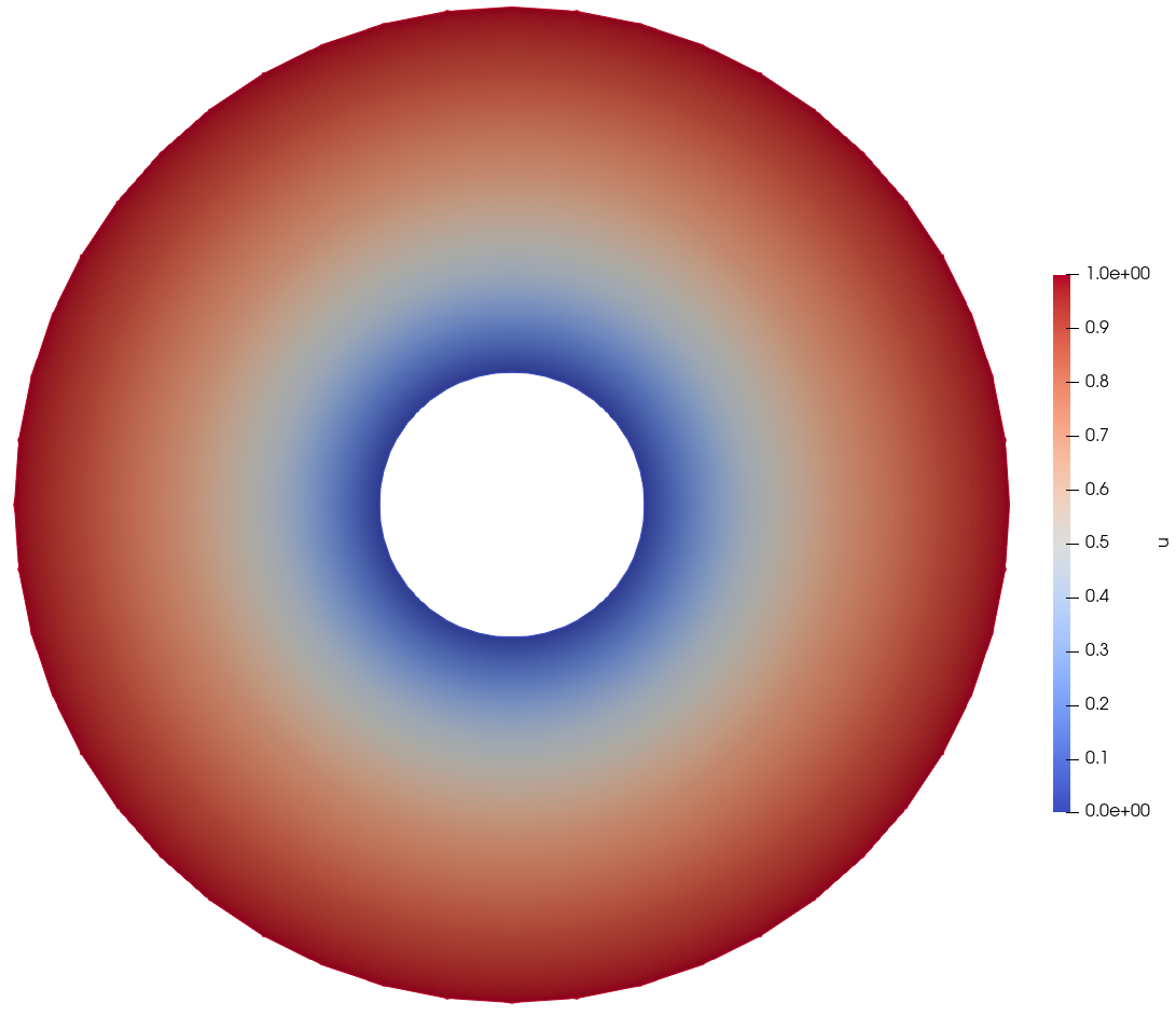
From diffusion_out.e in Paraview
Diffusion with Volumetric Source
Let's replace the outer boundary condition (Dirichlet setting ) with the natural boundary condition and then add a volumetric source represented by the function .
We will remove the DirichletBC named outer_dirichlet and add a new Kernel of type BodyForce.
Input: Diffusion with Volumetric Source
 @@ -1,39 +1,38 @@
 [Mesh<<<{"href": "../syntax/Mesh/index.html"}>>>/fuel_pin]
   type = FileMeshGenerator<<<{"description": "Read a mesh from a file.", "href": "../source/meshgenerators/FileMeshGenerator.html"}>>>
   file<<<{"description": "The filename to read."}>>> = ../step1_input_and_meshing/gold/fuel_pin_in.e
 []

 [Variables<<<{"href": "../syntax/Variables/index.html"}>>>]
   [u]
   []
 []

 [Kernels<<<{"href": "../syntax/Kernels/index.html"}>>>]
   [diffusion]
     type = Diffusion<<<{"description": "The Laplacian operator ($-\\nabla \\cdot \\nabla u$), with the weak form of $(\\nabla \\phi_i, \\nabla u_h)$.", "href": "../source/kernels/Diffusion.html"}>>>
     variable<<<{"description": "The name of the variable that this residual object operates on"}>>> = u
   []
+  [source]
+    type = BodyForce<<<{"description": "Demonstrates the multiple ways that scalar values can be introduced into kernels, e.g. (controllable) constants, functions, and postprocessors. Implements the weak form $(\\psi_i, -f)$.", "href": "../source/kernels/BodyForce.html"}>>>
+    variable<<<{"description": "The name of the variable that this residual object operates on"}>>> = u
+    function<<<{"description": "A function that describes the body force"}>>> = '1e9 * sqrt(x^2 + y^2)'
+  []
 []

 [BCs<<<{"href": "../syntax/BCs/index.html"}>>>]
   [inner_dirichlet]
     type = DirichletBC<<<{"description": "Imposes the essential boundary condition $u=g$, where $g$ is a constant, controllable value.", "href": "../source/bcs/DirichletBC.html"}>>>
     variable<<<{"description": "The name of the variable that this residual object operates on"}>>> = u
     boundary<<<{"description": "The list of boundary IDs from the mesh where this object applies"}>>> = inner
     value<<<{"description": "Value of the BC"}>>> = 0
-  []
-  [outer_dirichlet]
-    type = DirichletBC<<<{"description": "Imposes the essential boundary condition $u=g$, where $g$ is a constant, controllable value.", "href": "../source/bcs/DirichletBC.html"}>>>
-    variable<<<{"description": "The name of the variable that this residual object operates on"}>>> = u
-    boundary<<<{"description": "The list of boundary IDs from the mesh where this object applies"}>>> = water_solid_interface
-    value<<<{"description": "Value of the BC"}>>> = 1
   []
 []

 [Executioner<<<{"href": "../syntax/Executioner/index.html"}>>>]
   type = Steady
 []

 [Outputs<<<{"href": "../syntax/Outputs/index.html"}>>>]
   exodus<<<{"description": "Output the results using the default settings for Exodus output."}>>> = true
[](+ tutorials/user_short_workshop/inputs/step2_diffusion/diffusion_volumetric_source.i)
Run: Diffusion with Volumetric Source
$ moose-opt -i diffusion_volumetric_source.i
Result: Diffusion with Volumetric Source
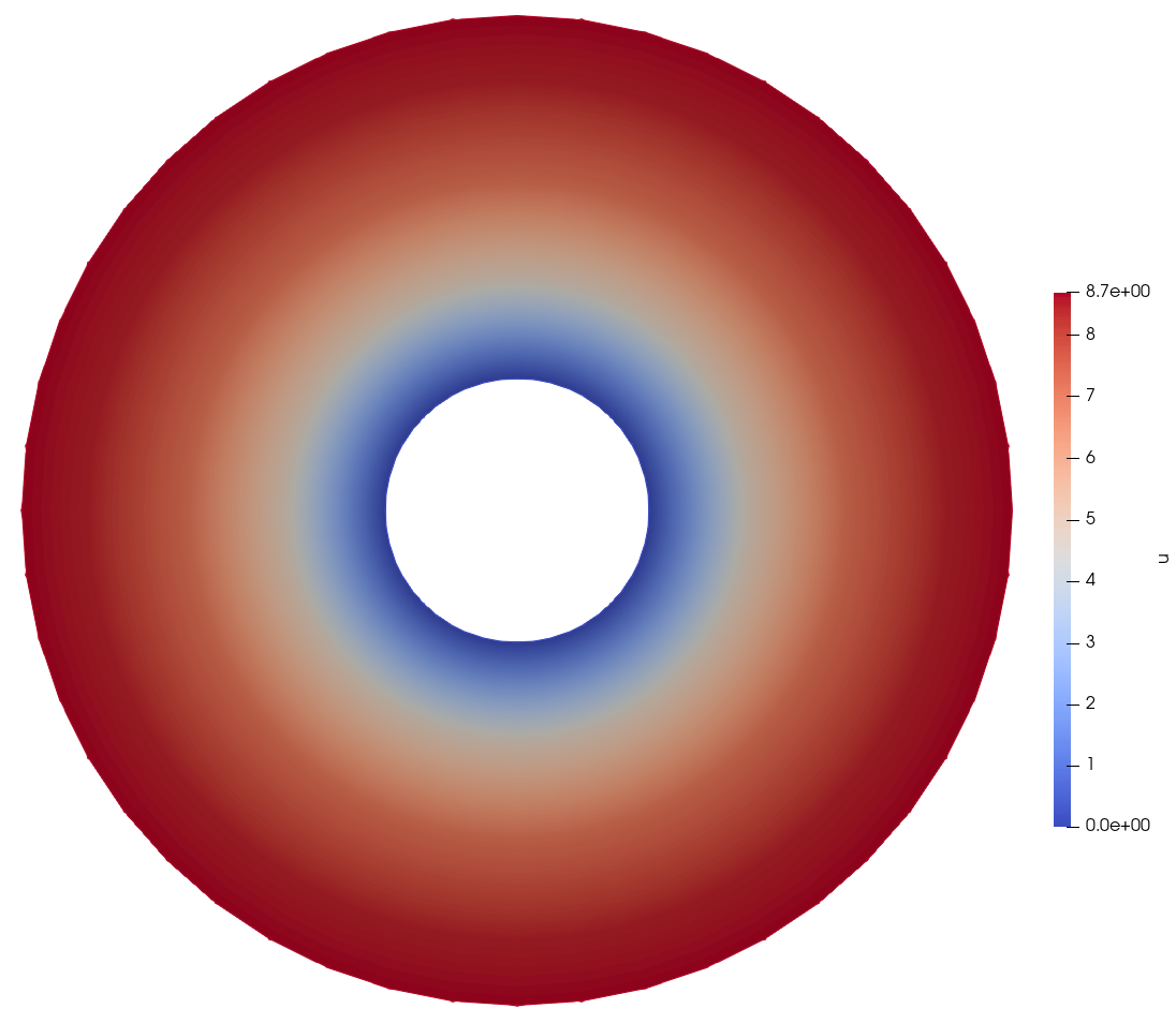
From diffusion_volumetric_source_out.e in Paraview
Step 3: Postprocessing
Postprocessor System
The PostProcessor system is used to aggregate data from a simulation.
Common use cases are:
Volumetric integration of a field
Variable averages
Surface integration of a field on a boundary
Flux on a boundary
Maximum and minimum values of a field
Other simulation information
Eigenvalues
Timing information
Solver properties
PostProcessor values are output in a table to screen and can also be output per timestep (and even per iteration) to a CSV file.
Diffusion Problem Postprocessing
For the simple diffusion problem in the previous step, the PostProcessor system will be used to output the average value of the solution variable on the outer boundary and within the fuel.
 @@ -1,39 +1,53 @@
 [Mesh<<<{"href": "../syntax/Mesh/index.html"}>>>/fuel_pin]
   type = FileMeshGenerator<<<{"description": "Read a mesh from a file.", "href": "../source/meshgenerators/FileMeshGenerator.html"}>>>
   file<<<{"description": "The filename to read."}>>> = ../step1_input_and_meshing/gold/fuel_pin_in.e
 []

 [Variables<<<{"href": "../syntax/Variables/index.html"}>>>]
   [u]
   []
 []

 [Kernels<<<{"href": "../syntax/Kernels/index.html"}>>>]
   [diffusion]
     type = Diffusion<<<{"description": "The Laplacian operator ($-\\nabla \\cdot \\nabla u$), with the weak form of $(\\nabla \\phi_i, \\nabla u_h)$.", "href": "../source/kernels/Diffusion.html"}>>>
     variable<<<{"description": "The name of the variable that this residual object operates on"}>>> = u
   []
 []

 [BCs<<<{"href": "../syntax/BCs/index.html"}>>>]
   [inner_dirichlet]
     type = DirichletBC<<<{"description": "Imposes the essential boundary condition $u=g$, where $g$ is a constant, controllable value.", "href": "../source/bcs/DirichletBC.html"}>>>
     variable<<<{"description": "The name of the variable that this residual object operates on"}>>> = u
     boundary<<<{"description": "The list of boundary IDs from the mesh where this object applies"}>>> = inner
     value<<<{"description": "Value of the BC"}>>> = 0
   []
   [outer_dirichlet]
     type = DirichletBC<<<{"description": "Imposes the essential boundary condition $u=g$, where $g$ is a constant, controllable value.", "href": "../source/bcs/DirichletBC.html"}>>>
     variable<<<{"description": "The name of the variable that this residual object operates on"}>>> = u
     boundary<<<{"description": "The list of boundary IDs from the mesh where this object applies"}>>> = water_solid_interface
     value<<<{"description": "Value of the BC"}>>> = 1
   []
 []

+[Postprocessors<<<{"href": "../syntax/Postprocessors/index.html"}>>>]
+  [fuel_average]
+    type = ElementAverageValue<<<{"description": "Computes the volumetric average of a variable", "href": "../source/postprocessors/ElementAverageValue.html"}>>>
+    variable<<<{"description": "The name of the variable that this object operates on"}>>> = u
+    block<<<{"description": "The list of blocks (ids or names) that this object will be applied"}>>> = fuel
+  []
+  [outer_average]
+    type = SideAverageValue<<<{"description": "Computes the average value of a variable on a sideset. Note that this cannot be used on the centerline of an axisymmetric model.", "href": "../source/postprocessors/SideAverageValue.html"}>>>
+    variable<<<{"description": "The name of the variable which this postprocessor integrates"}>>> = u
+    boundary<<<{"description": "The list of boundary IDs from the mesh where this object applies"}>>> = water_solid_interface
+  []
+[]
+
 [Executioner<<<{"href": "../syntax/Executioner/index.html"}>>>]
   type = Steady
 []

 [Outputs<<<{"href": "../syntax/Outputs/index.html"}>>>]
   exodus<<<{"description": "Output the results using the default settings for Exodus output."}>>> = true
+  csv<<<{"description": "Output the scalar variable and postprocessors to a *.csv file using the default CSV output."}>>> = true
[](+ tutorials/user_short_workshop/inputs/step3_postprocessing/postprocessing.i)
Run: Diffusion Problem Postprocessing
$ cd ../step3_postprocessing
$ moose-opt -i postprocessing.i
At the end of the simulation, the postprocessor values appear on screen:
Postprocessor Values:
+----------------+----------------+----------------+
| time           | fuel_average   | outer_average  |
+----------------+----------------+----------------+
|   0.000000e+00 |   0.000000e+00 |   0.000000e+00 |
|   1.000000e+00 |   5.951556e-01 |   1.000000e+00 |
+----------------+----------------+----------------+
You may also open the postprocessing_out.csv file to view the csv contents.
Step 4: Materials
Materials
Realistic problems have spatially dependent properties. Often these properties are also shared across equations (or Variables, in MOOSE world).
In MOOSE, these properties are defined using the Materials system:
Material objects produce one or more named "material properties" on quadrature points
The values are computed on-demand (during residual and Jacobian evaluation)
Material properties can be of any type (scalars, vector values, etc)
Can be restricted to blocks for spatial variation
Can consume variable values (ex: fluid properties depend on )
Can depend on other materials (adds execution dependencies)
Can optionally propagate derivatives through automatic differentiation
Objects like Kernels then consume material properties. This pluggable design enables the convenient sharing of material properties in a well-defined manner.
Spatially-Dependent Diffusion
We will take our previous diffusion solve and introduce coefficients of the diffusivity to the fuel region (block fuel, of value ) and the cladding region (block clad, of value ). The previous coefficient of diffusivity was for both regions.
This will require two changes:
Replacing the
Diffusionkernel with aMatDiffusionkernel, which consumes a material property namedDfor the diffusion coefficientAdding two
GenericConstantMaterialMaterial objects, one for each of the two blocks
Input: Spatially-Dependent Diffusion
 @@ -1,39 +1,54 @@
 [Mesh<<<{"href": "../syntax/Mesh/index.html"}>>>/fuel_pin]
   type = FileMeshGenerator<<<{"description": "Read a mesh from a file.", "href": "../source/meshgenerators/FileMeshGenerator.html"}>>>
   file<<<{"description": "The filename to read."}>>> = ../step1_input_and_meshing/gold/fuel_pin_in.e
 []

 [Variables<<<{"href": "../syntax/Variables/index.html"}>>>]
   [u]
   []
 []

 [Kernels<<<{"href": "../syntax/Kernels/index.html"}>>>]
   [diffusion]
-    type = Diffusion<<<{"description": "The Laplacian operator ($-\\nabla \\cdot \\nabla u$), with the weak form of $(\\nabla \\phi_i, \\nabla u_h)$.", "href": "../source/kernels/Diffusion.html"}>>>
+    type = MatDiffusion<<<{"description": "Diffusion equation Kernel that takes an isotropic Diffusivity from a material property", "href": "../source/kernels/MatDiffusion.html"}>>>
     variable<<<{"description": "The name of the variable that this residual object operates on"}>>> = u
   []
 []

 [BCs<<<{"href": "../syntax/BCs/index.html"}>>>]
   [inner_dirichlet]
     type = DirichletBC<<<{"description": "Imposes the essential boundary condition $u=g$, where $g$ is a constant, controllable value.", "href": "../source/bcs/DirichletBC.html"}>>>
     variable<<<{"description": "The name of the variable that this residual object operates on"}>>> = u
     boundary<<<{"description": "The list of boundary IDs from the mesh where this object applies"}>>> = inner
     value<<<{"description": "Value of the BC"}>>> = 0
   []
   [outer_dirichlet]
     type = DirichletBC<<<{"description": "Imposes the essential boundary condition $u=g$, where $g$ is a constant, controllable value.", "href": "../source/bcs/DirichletBC.html"}>>>
     variable<<<{"description": "The name of the variable that this residual object operates on"}>>> = u
     boundary<<<{"description": "The list of boundary IDs from the mesh where this object applies"}>>> = water_solid_interface
     value<<<{"description": "Value of the BC"}>>> = 1
   []
 []

+[Materials<<<{"href": "../syntax/Materials/index.html"}>>>]
+  [D_fuel]
+    type = GenericConstantMaterial<<<{"description": "Declares material properties based on names and values prescribed by input parameters.", "href": "../source/materials/GenericConstantMaterial.html"}>>>
+    prop_names<<<{"description": "The names of the properties this material will have"}>>> = D
+    prop_values<<<{"description": "The values associated with the named properties"}>>> = 100
+    block<<<{"description": "The list of blocks (ids or names) that this object will be applied"}>>> = fuel
+  []
+  [D_clad]
+    type = GenericConstantMaterial<<<{"description": "Declares material properties based on names and values prescribed by input parameters.", "href": "../source/materials/GenericConstantMaterial.html"}>>>
+    prop_names<<<{"description": "The names of the properties this material will have"}>>> = D
+    prop_values<<<{"description": "The values associated with the named properties"}>>> = 2
+    block<<<{"description": "The list of blocks (ids or names) that this object will be applied"}>>> = clad
+  []
+[]
+
 [Executioner<<<{"href": "../syntax/Executioner/index.html"}>>>]
   type = Steady
 []

 [Outputs<<<{"href": "../syntax/Outputs/index.html"}>>>]
   exodus<<<{"description": "Output the results using the default settings for Exodus output."}>>> = true
[](+ tutorials/user_short_workshop/inputs/step4_materials/diffusion_materials.i)
Run: Spatially-Dependent Diffusion
$ cd ../step4_materials
$ moose-opt -i diffusion_materials.i
Result: Spatially-Dependent Diffusion
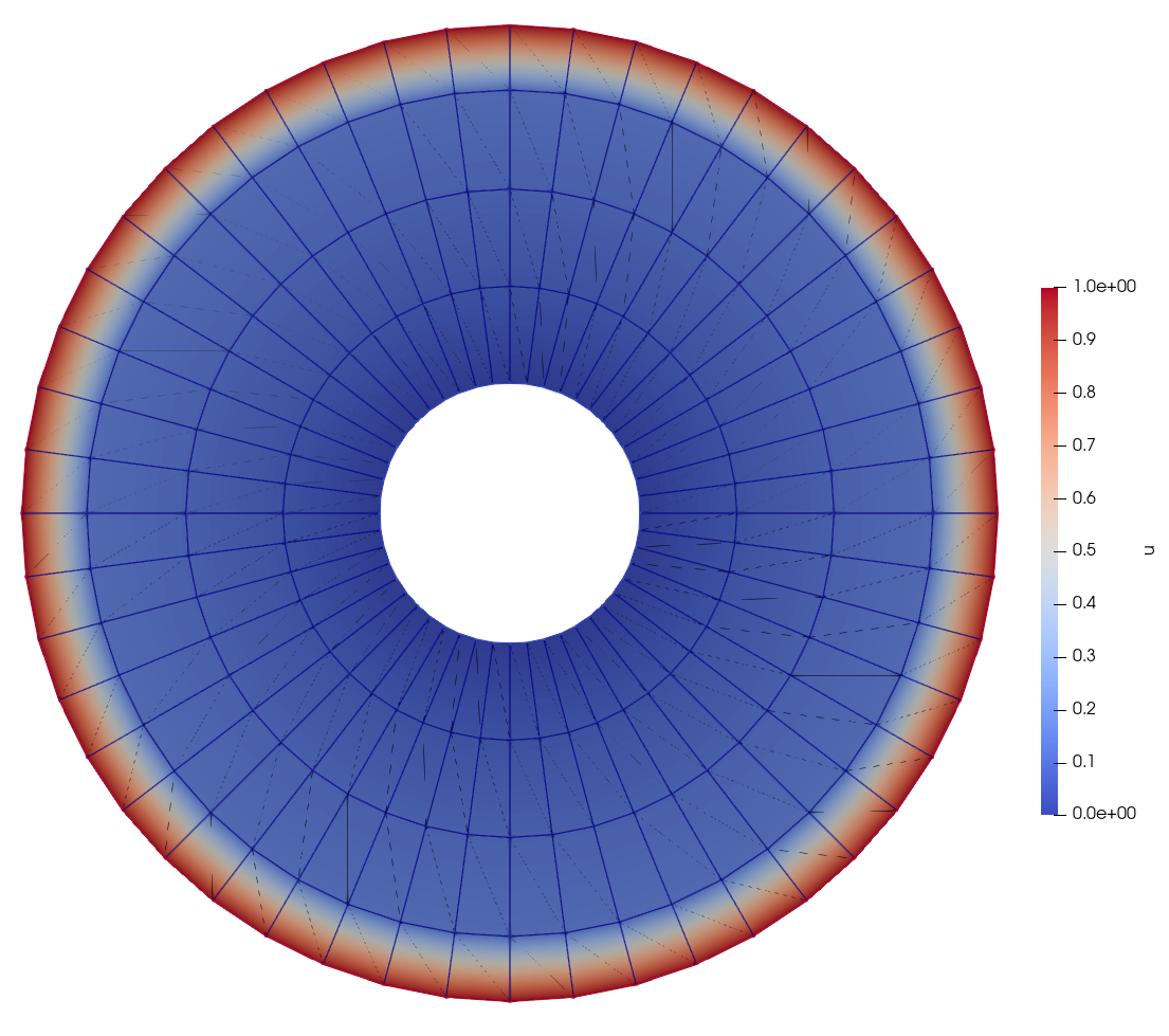
From diffusion_materials_out.e in Paraview
Result: Spatially-Dependent Diffusion Line
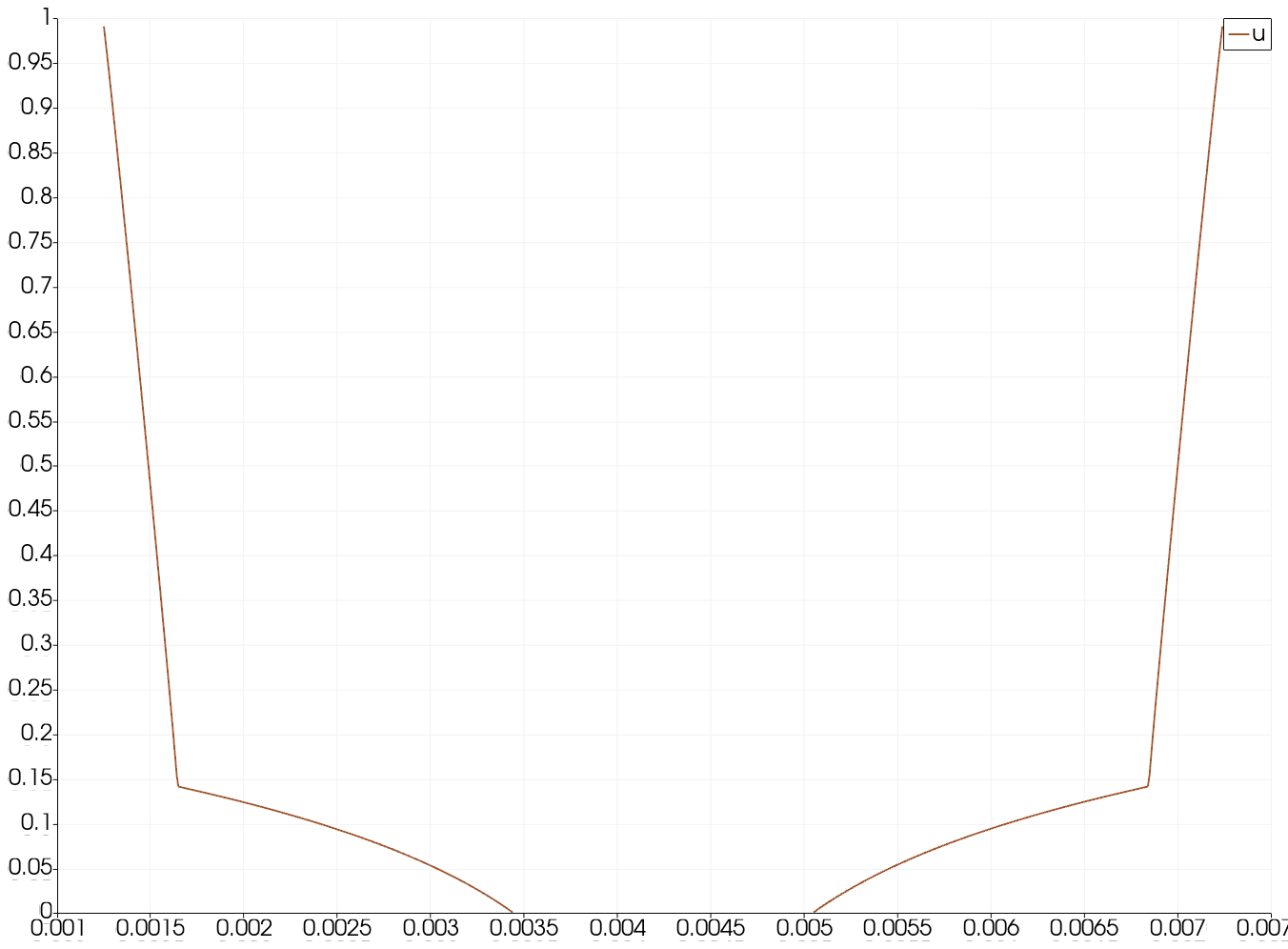
Line plot of through from diffusion_materials_out.e in Paraview with refinement
Step 5: Heat Conduction
Solid Heat Conduction
Thus far, we've solved the diffusion problem on our pin cell with heterogeneity between the clad and the fuel. Let's solve something a little more realistic. We will solve a heat conduction problem on the same solid geometry where:
The outer boundary (
water_solid_interface) has a prescribed temperature of KThe inner boundary has zero heat flux
There is a volumetric heat source in the fuel (
fuel) of
The material properties are as follows:
| Property | Fuel | Clad |
|---|---|---|
| 2 W/m | 10 W/m | |
| 3100 J/(kg-K) | 2800 J/(kg-K) | |
| 10700 kg/m | 5400 kg/m |
Additional Capabilities
A few new things will be introduced in this step:
Physicssystem: for setting up a heat conduction problem using the conveniencePhysics/HeatConduction/FiniteElementsyntaxAuxVariablesystem: for defining fields that are auxiliary (not solved for)AuxKernelsystem: for filling anAuxVariable
Auxiliary Variables and Kernels
The term "auxiliary variable" is defined, in MOOSE language, as a variable that is directly calculated using an AuxKernel object. An AuxKernel fills into an AuxVariable. This allows for postprocessing, coupling, and proxy calculations.
Auxiliary variables come in two flavors:
Elemental: constant or higher-order monomials; discontinuous across elements
Nodal: like linear-lagrange; continuous across elements
In particular, we will utilize the DiffusionFluxAux to compute the integral of the heat flux on the outer boundary (water_solid_interface).
We will also use an AuxVariable named T_fluid to define the field that is used as the outer boundary condition.
Input: Solid Heat Conduction
[Mesh<<<{"href": "../syntax/Mesh/index.html"}>>>/fuel_pin]
  type = FileMeshGenerator<<<{"description": "Read a mesh from a file.", "href": "../source/meshgenerators/FileMeshGenerator.html"}>>>
  file<<<{"description": "The filename to read."}>>> = ../step1_input_and_meshing/gold/fuel_pin_in.e
[]

[Physics<<<{"href": "../syntax/Physics/index.html"}>>>/HeatConduction<<<{"href": "../syntax/Physics/HeatConduction/index.html"}>>>/FiniteElement<<<{"href": "../syntax/Physics/HeatConduction/FiniteElement/index.html"}>>>/heat_conduction]
  # Solve heat conduction on fuel and cladding
  block<<<{"description": "Blocks (subdomains) that this Physics is active on."}>>> = 'fuel clad'

  # Store temperature as the variable "T"
  temperature_name<<<{"description": "Variable name for the temperature"}>>> = T

  # Fix the outer boundary temperature to the
  # fluid boundary temperature, pulled in from
  # the aux variable "T_fluid"
  # (for now is the value 300 K)
  fixed_temperature_boundaries<<<{"description": "Boundaries on which to apply a fixed temperature"}>>> = water_solid_interface
  boundary_temperatures<<<{"description": "Functors to compute the heat flux on each boundary in 'fixed_temperature_boundaries'. A functor is any of the following: a variable, a functor material property, a function, a postprocessor or a number."}>>> = T_fluid # [K]

  # Insulate the inner boundary (zero heat flux)
  insulated_boundaries<<<{"description": "Boundaries on which to apply a zero heat flux"}>>> = inner

  # Name of the material properties
  thermal_conductivity<<<{"description": "the name of the thermal conductivity material property"}>>> = k
  specific_heat<<<{"description": "Name of the volumetric isobaric specific heat material property"}>>> = cp
  density<<<{"description": "Density material property"}>>> = rho

  # Numerical parameters
  use_automatic_differentiation<<<{"description": "Whether to use automatic differentiation for all the terms in the equation"}>>> = false
[]

# Apply a constant heat source to the fuel
[Kernels<<<{"href": "../syntax/Kernels/index.html"}>>>/heat_source]
  type = BodyForce<<<{"description": "Demonstrates the multiple ways that scalar values can be introduced into kernels, e.g. (controllable) constants, functions, and postprocessors. Implements the weak form $(\\psi_i, -f)$.", "href": "../source/kernels/BodyForce.html"}>>>
  variable<<<{"description": "The name of the variable that this residual object operates on"}>>> = T
  value<<<{"description": "Coefficient to multiply by the body force term"}>>> = 1e8 # [W/m^3]
[]

[Materials<<<{"href": "../syntax/Materials/index.html"}>>>]
  [fuel]
    type = GenericConstantMaterial<<<{"description": "Declares material properties based on names and values prescribed by input parameters.", "href": "../source/materials/GenericConstantMaterial.html"}>>>
    prop_names<<<{"description": "The names of the properties this material will have"}>>> = 'k cp rho'
    prop_values<<<{"description": "The values associated with the named properties"}>>> = '2 3100 10700' # [W/(m-K)], [J/(kg-K)], [kg/m^3]
    block<<<{"description": "The list of blocks (ids or names) that this object will be applied"}>>> = fuel
  []
  [clad]
    type = GenericConstantMaterial<<<{"description": "Declares material properties based on names and values prescribed by input parameters.", "href": "../source/materials/GenericConstantMaterial.html"}>>>
    prop_names<<<{"description": "The names of the properties this material will have"}>>> = 'k cp rho'
    prop_values<<<{"description": "The values associated with the named properties"}>>> = '10 2800 5400' # [W/(m-K)], [J/(kg-K)], [kg/m^3]
    block<<<{"description": "The list of blocks (ids or names) that this object will be applied"}>>> = clad
  []
[]

[AuxVariables<<<{"href": "../syntax/AuxVariables/index.html"}>>>]
  # Define an aux field variable that stores the temperature of
  # fluid on the outer boundary
  [T_fluid]
    initial_condition<<<{"description": "Specifies a constant initial condition for this variable"}>>> = 300 # [K]
    block = clad
  []
  # Define an aux field variable that stores the heat flux
  # on the outer boundary (the fluid interface)
  # To store the heat flux computation
  [heat_flux]
    # We compute the heat flux on the boundary cell
    # centers rather than nodes because linear-Lagrange
    # T does not have a well-defined gradient at nodes
    order<<<{"description": "Specifies the order of the FE shape function to use for this variable (additional orders not listed are allowed)"}>>> = CONSTANT
    family<<<{"description": "Specifies the family of FE shape functions to use for this variable"}>>> = MONOMIAL
    block = clad
  []
[]

# Define an aux kernel that fills in the heat
# flux at the outer interface
[AuxKernels<<<{"href": "../syntax/AuxKernels/index.html"}>>>/heat_flux]
  type = DiffusionFluxAux<<<{"description": "Compute components of flux vector for diffusion problems $(\\vec{J} = -D \\nabla C)$.", "href": "../source/auxkernels/DiffusionFluxAux.html"}>>>
  variable<<<{"description": "The name of the variable that this object applies to"}>>> = heat_flux
  diffusivity<<<{"description": "The name of the diffusivity material property that will be used in the flux computation."}>>> = k
  diffusion_variable<<<{"description": "The name of the variable"}>>> = T
  boundary<<<{"description": "The list of boundaries (ids or names) from the mesh where this object applies"}>>> = 'water_solid_interface'
  component<<<{"description": "The desired component of flux."}>>> = normal
[]

[Postprocessors<<<{"href": "../syntax/Postprocessors/index.html"}>>>]
  # Compute the maximum temperature
  [T_max]
    type = NodalExtremeValue<<<{"description": "Finds either the min or max elemental value of a variable over the domain.", "href": "../source/postprocessors/NodalExtremeValue.html"}>>>
    variable<<<{"description": "The name of the variable that this postprocessor operates on"}>>> = T
  []

  # Compute the integral of the outgoing heat flux
  [heat_flux_integral]
    type = SideIntegralVariablePostprocessor<<<{"description": "Computes a surface integral of the specified variable", "href": "../source/postprocessors/SideIntegralVariablePostprocessor.html"}>>>
    variable<<<{"description": "The name of the variable which this postprocessor integrates"}>>> = heat_flux
    boundary<<<{"description": "The list of boundary IDs from the mesh where this object applies"}>>> = 'water_solid_interface'
  []
[]

[Executioner<<<{"href": "../syntax/Executioner/index.html"}>>>]
  type = Steady
[]

[Outputs<<<{"href": "../syntax/Outputs/index.html"}>>>]
  exodus<<<{"description": "Output the results using the default settings for Exodus output."}>>> = true
  csv<<<{"description": "Output the scalar variable and postprocessors to a *.csv file using the default CSV output."}>>> = true
[]Run: Solid Heat Conduction
$ cd ../step5_heat_conduction
$ moose-opt -i solid.i
Postprocessor Values:
+----------------+----------------+--------------------+
| time           | T_max          | heat_flux_integral |
+----------------+----------------+--------------------+
|   0.000000e+00 |   0.000000e+00 |       0.000000e+00 |
|   1.000000e+00 |   3.636917e+02 |       2.421074e+03 |
+----------------+----------------+--------------------+
Result: Solid Heat Conduction
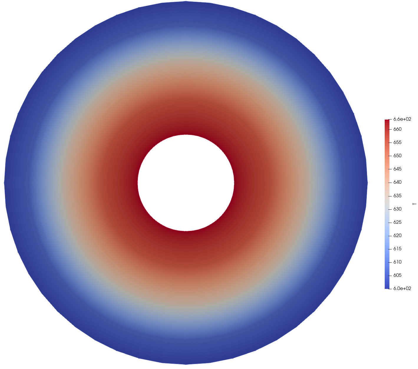
From solid_out.e in Paraview
Result: Solid Heat Conduction Line
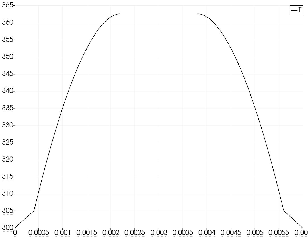
Line plot of through from solid_out.e in Paraview with refinement
Fluid Heat Conduction
Recall our "fluid" mesh from Step 1: Input and Meshing:
Fluid Heat Conduction
It will become clear why in the next step – but let's also solve a heat conduction problem on our fluid mesh with the following:
The outer boundary (
outer) has a prescribed temperature ofThe inner boundary (
water_solid_interface) has a Neumann boundary condition that fixes the incoming heat flux to a value of
The material properties are as follows:
| Property | Value |
|---|---|
| 0.6 W/m | |
| 1000 J/(kg-K) | |
| 4100 kg/m |
Input: Fluid Heat Conduction
[Mesh<<<{"href": "../syntax/Mesh/index.html"}>>>/fluid]
  type = FileMeshGenerator<<<{"description": "Read a mesh from a file.", "href": "../source/meshgenerators/FileMeshGenerator.html"}>>>
  file<<<{"description": "The filename to read."}>>> = ../step1_input_and_meshing/gold/fluid_in.e
[]

[Physics<<<{"href": "../syntax/Physics/index.html"}>>>/HeatConduction<<<{"href": "../syntax/Physics/HeatConduction/index.html"}>>>/FiniteElement<<<{"href": "../syntax/Physics/HeatConduction/FiniteElement/index.html"}>>>/heat_conduction]
  # Solve heat conduction on the water
  block<<<{"description": "Blocks (subdomains) that this Physics is active on."}>>> = 'water'

  # Store temperature as the variable "T"
  temperature_name<<<{"description": "Variable name for the temperature"}>>> = T

  # Prescribe the heat flux on the water solid
  # interface to that from the interface, pulled
  # in from the aux variable "flux_from_solid"
  heat_flux_boundaries<<<{"description": "Boundaries on which to apply a heat flux"}>>> = water_solid_interface
  boundary_heat_fluxes<<<{"description": "Functors to compute the heat flux on each boundary in 'heat_flux_boundaries'. A functor is any of the following: a variable, a functor material property, a function, a postprocessor or a number."}>>> = flux_from_solid # [W/m^2]

  # Evacuate heat at the outer boundary
  # with a prescribed temperature of 300 K
  fixed_temperature_boundaries<<<{"description": "Boundaries on which to apply a fixed temperature"}>>> = outer
  boundary_temperatures<<<{"description": "Functors to compute the heat flux on each boundary in 'fixed_temperature_boundaries'. A functor is any of the following: a variable, a functor material property, a function, a postprocessor or a number."}>>> = 300 # [K]

  # Name of the material properties
  thermal_conductivity<<<{"description": "the name of the thermal conductivity material property"}>>> = k
  specific_heat<<<{"description": "Name of the volumetric isobaric specific heat material property"}>>> = cp
  density<<<{"description": "Density material property"}>>> = rho
[]

# Define a field variable that stores the heat
# flux from the solid
[AuxVariables<<<{"href": "../syntax/AuxVariables/index.html"}>>>]
  [flux_from_solid]
    initial_condition<<<{"description": "Specifies a constant initial condition for this variable"}>>> = 2e4 # [W/m^2]
  []
[]

[Materials<<<{"href": "../syntax/Materials/index.html"}>>>]
  [k_water]
    type = ADGenericConstantMaterial<<<{"description": "Declares material properties based on names and values prescribed by input parameters.", "href": "../source/materials/GenericConstantMaterial.html"}>>>
    prop_names<<<{"description": "The names of the properties this material will have"}>>> = 'k rho cp'
    prop_values<<<{"description": "The values associated with the named properties"}>>> = '0.6 1000 4100'
    block<<<{"description": "The list of blocks (ids or names) that this object will be applied"}>>> = water
  []
[]

[Executioner<<<{"href": "../syntax/Executioner/index.html"}>>>]
  type = Steady
[]

[Outputs<<<{"href": "../syntax/Outputs/index.html"}>>>]
  exodus<<<{"description": "Output the results using the default settings for Exodus output."}>>> = true
[]Run: Fluid Heat Conduction
$ moose-opt -i fluid.i
Result: Fluid Heat Conduction
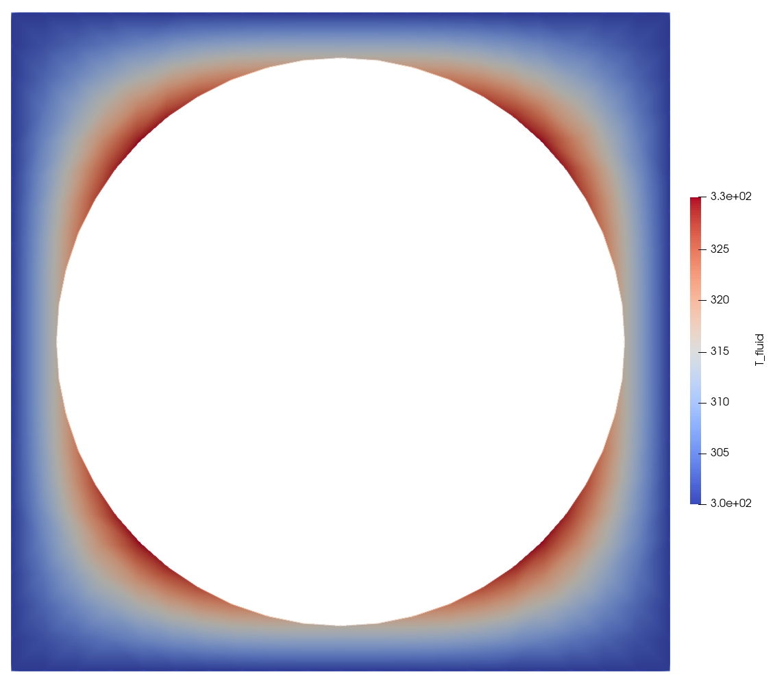
From fluid_out.e in Paraview
Step 6: Coupling
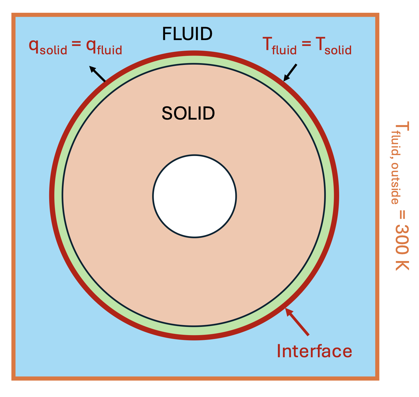
Coupling Problem
Next, we will couple our fluid and solid (fuel pin) systems together at the interface between the two meshes (along the water_solid_interface boundary in each problem).
This aims to be an example of multiphysics coupling within MOOSE. Note that it isn't a true multiphysics simulation, but it is an example on the use of the MultiApp system and the Transfer system.
The two inputs that were created in Step 5: Heat Conduction will be extended in this problem.
Problem Definition
MultiApp System
MOOSE was originally created to solve fully-coupled systems of partial differential equations (PDEs). Systems of PDEs in MOOSE can be solved either tightly-coupled or loosely-coupled:
Tight coupling can be accomplished by solving multiple PDEs in a single matrix system, or via operator-splitting plus fixed point iteration
Multiscale systems are generally loosely coupled between scales
Systems with both fast and slow physics can be decoupled in time
A MultiApp allows you to simultaneously solve for individual physics systems.
You can think of a MultiApp of an instantiation (or many instantiations!) of another input file that can be executed during the main application's solve.
MultiApp Input Example
[MultiApps/fluid]
  type = TransientMultiApp
  input_files = 'fluid.i'
  execute_on = TIMESTEP_END
[]
Transfer System
A Transfer describes how you move information up and down the MultiApp hierarchy.
There are three common ways a Transfer can read information and deposit information:
Variable(read only) andAuxVariablefieldsPostProcessorvaluesUserObjectinformation (not discussed here)
By having MOOSE move data and fill fields... apps don't need to know or care where the data came from or how it got there!
Transfer Input Example
[Transfers/send_heat_flux]
  type = MultiAppGeneralFieldNearestLocationTransfer
  from_multi_app = fluid
  source_variable = T_fluid
  variable = T_fluid
  to_boundaries = water_solid_interface
[]
Problem Definition
Problem MultiApp Summary
We will have two input files: solid.i and fluid.i. The solid (fuel pin) input will the "main" input, thus the fluid input will have a MultiApp.
This will require a single [MultiApp] in solid.i (for fluid.i) and two transfers in solid.i:
The transfer of the heat flux from the solid to the fluid on the periphery of the clad (the
water_solid_interfaceboundary)The transfer of the fluid temperature on its inner interface (also
water_solid_interface) to the solid
Problem MultiApp Block
[MultiApps<<<{"href": "../syntax/MultiApps/index.html"}>>>]
  [fluid]
    type = TransientMultiApp<<<{"description": "MultiApp for performing coupled simulations with the parent and sub-application both progressing in time.", "href": "../source/multiapps/TransientMultiApp.html"}>>>
    input_files<<<{"description": "The input file for each App.  If this parameter only contains one input file it will be used for all of the Apps.  When using 'positions_from_file' it is also admissable to provide one input_file per file."}>>> = fluid.i

    # Couple at the end of each timestep
    execute_on<<<{"description": "The list of flag(s) indicating when this object should be executed. For a description of each flag, see https://mooseframework.inl.gov/source/interfaces/SetupInterface.html."}>>> = TIMESTEP_END

    no_restore<<<{"description": "True to turn off restore for this multiapp. This is useful when doing steady-state Picard iterations where we want to use the solution of previous Picard iteration as the initial guess of the current Picard iteration."}>>> = true
  []
[]Problem Transfers Block
[Transfers<<<{"href": "../syntax/Transfers/index.html"}>>>]
  # Send the outgoing heat flux from the solid problem
  # at the end of each timestep
  [send_heat_flux]
    type = MultiAppGeneralFieldNearestLocationTransfer<<<{"description": "Transfers field data at the MultiApp position by finding the value at the nearest neighbor(s) in the origin application.", "href": "../source/transfers/MultiAppGeneralFieldNearestLocationTransfer.html"}>>>
    to_multi_app<<<{"description": "The name of the MultiApp to transfer the data to"}>>> = fluid
    source_variable<<<{"description": "The variable to transfer from."}>>> = 'heat_flux'
    variable<<<{"description": "The auxiliary variable to store the transferred values in."}>>> = 'flux_from_solid'
    to_boundaries<<<{"description": "The boundary we are transferring to (if not specified, whole domain is used)."}>>> = 'water_solid_interface'
  []
  # Receive the fluid temperature field from the
  # fluid multiapp at the end of each timestep
  [receive_Tfluid]
    type = MultiAppGeneralFieldNearestLocationTransfer<<<{"description": "Transfers field data at the MultiApp position by finding the value at the nearest neighbor(s) in the origin application.", "href": "../source/transfers/MultiAppGeneralFieldNearestLocationTransfer.html"}>>>
    from_multi_app<<<{"description": "The name of the MultiApp to receive data from"}>>> = fluid
    source_variable<<<{"description": "The variable to transfer from."}>>> = 'T'
    variable<<<{"description": "The auxiliary variable to store the transferred values in."}>>> = 'T_fluid'
    to_boundaries<<<{"description": "The boundary we are transferring to (if not specified, whole domain is used)."}>>> = 'water_solid_interface'
  []
[]Problem Input: Solid
 @@ -1,107 +1,161 @@
 [Mesh<<<{"href": "../syntax/Mesh/index.html"}>>>/fuel_pin]
   type = FileMeshGenerator<<<{"description": "Read a mesh from a file.", "href": "../source/meshgenerators/FileMeshGenerator.html"}>>>
   file<<<{"description": "The filename to read."}>>> = ../step1_input_and_meshing/gold/fuel_pin_in.e
 []

 [Physics<<<{"href": "../syntax/Physics/index.html"}>>>/HeatConduction<<<{"href": "../syntax/Physics/HeatConduction/index.html"}>>>/FiniteElement<<<{"href": "../syntax/Physics/HeatConduction/FiniteElement/index.html"}>>>/heat_conduction]
   # Solve heat conduction on fuel and cladding
   block<<<{"description": "Blocks (subdomains) that this Physics is active on."}>>> = 'fuel clad'

   # Store temperature as the variable "T"
   temperature_name<<<{"description": "Variable name for the temperature"}>>> = T
+  # With an initial temperature of 310 K
+  initial_temperature<<<{"description": "Initial value of the temperature variable"}>>> = 310 # [K]

   # Fix the outer boundary temperature to the
   # fluid boundary temperature, pulled in from
   # the aux variable "T_fluid"
   # (for now is the value 300 K)
   fixed_temperature_boundaries<<<{"description": "Boundaries on which to apply a fixed temperature"}>>> = water_solid_interface
   boundary_temperatures<<<{"description": "Functors to compute the heat flux on each boundary in 'fixed_temperature_boundaries'. A functor is any of the following: a variable, a functor material property, a function, a postprocessor or a number."}>>> = T_fluid # [K]

   # Insulate the inner boundary (zero heat flux)
   insulated_boundaries<<<{"description": "Boundaries on which to apply a zero heat flux"}>>> = inner

   # Name of the material properties
   thermal_conductivity<<<{"description": "the name of the thermal conductivity material property"}>>> = k
   specific_heat<<<{"description": "Name of the volumetric isobaric specific heat material property"}>>> = cp
   density<<<{"description": "Density material property"}>>> = rho

   # Numerical parameters
   use_automatic_differentiation<<<{"description": "Whether to use automatic differentiation for all the terms in the equation"}>>> = false
 []

 # Apply a constant heat source to the fuel
 [Kernels<<<{"href": "../syntax/Kernels/index.html"}>>>/heat_source]
   type = BodyForce<<<{"description": "Demonstrates the multiple ways that scalar values can be introduced into kernels, e.g. (controllable) constants, functions, and postprocessors. Implements the weak form $(\\psi_i, -f)$.", "href": "../source/kernels/BodyForce.html"}>>>
   variable<<<{"description": "The name of the variable that this residual object operates on"}>>> = T
   value<<<{"description": "Coefficient to multiply by the body force term"}>>> = 1e8 # [W/m^3]
 []

 [Materials<<<{"href": "../syntax/Materials/index.html"}>>>]
   [fuel]
     type = GenericConstantMaterial<<<{"description": "Declares material properties based on names and values prescribed by input parameters.", "href": "../source/materials/GenericConstantMaterial.html"}>>>
     prop_names<<<{"description": "The names of the properties this material will have"}>>> = 'k cp rho'
     prop_values<<<{"description": "The values associated with the named properties"}>>> = '2 3100 10700' # [W/(m-K)], [J/(kg-K)], [kg/m^3]
     block<<<{"description": "The list of blocks (ids or names) that this object will be applied"}>>> = fuel
   []
   [clad]
     type = GenericConstantMaterial<<<{"description": "Declares material properties based on names and values prescribed by input parameters.", "href": "../source/materials/GenericConstantMaterial.html"}>>>
     prop_names<<<{"description": "The names of the properties this material will have"}>>> = 'k cp rho'
     prop_values<<<{"description": "The values associated with the named properties"}>>> = '10 2800 5400' # [W/(m-K)], [J/(kg-K)], [kg/m^3]
     block<<<{"description": "The list of blocks (ids or names) that this object will be applied"}>>> = clad
   []
 []

 [AuxVariables<<<{"href": "../syntax/AuxVariables/index.html"}>>>]
   # Define an aux field variable that stores the temperature of
   # fluid on the outer boundary
   [T_fluid]
     initial_condition<<<{"description": "Specifies a constant initial condition for this variable"}>>> = 300 # [K]
     block = clad
   []
   # Define an aux field variable that stores the heat flux
   # on the outer boundary (the fluid interface)
   # To store the heat flux computation
   [heat_flux]
     # We compute the heat flux on the boundary cell
     # centers rather than nodes because linear-Lagrange
     # T does not have a well-defined gradient at nodes
     order<<<{"description": "Specifies the order of the FE shape function to use for this variable (additional orders not listed are allowed)"}>>> = CONSTANT
     family<<<{"description": "Specifies the family of FE shape functions to use for this variable"}>>> = MONOMIAL
     block = clad
   []
 []

 # Define an aux kernel that fills in the heat
 # flux at the outer interface
 [AuxKernels<<<{"href": "../syntax/AuxKernels/index.html"}>>>/heat_flux]
   type = DiffusionFluxAux<<<{"description": "Compute components of flux vector for diffusion problems $(\\vec{J} = -D \\nabla C)$.", "href": "../source/auxkernels/DiffusionFluxAux.html"}>>>
   variable<<<{"description": "The name of the variable that this object applies to"}>>> = heat_flux
   diffusivity<<<{"description": "The name of the diffusivity material property that will be used in the flux computation."}>>> = k
   diffusion_variable<<<{"description": "The name of the variable"}>>> = T
   boundary<<<{"description": "The list of boundaries (ids or names) from the mesh where this object applies"}>>> = 'water_solid_interface'
   component<<<{"description": "The desired component of flux."}>>> = normal
 []

 [Postprocessors<<<{"href": "../syntax/Postprocessors/index.html"}>>>]
   # Compute the maximum temperature
   [T_max]
     type = NodalExtremeValue<<<{"description": "Finds either the min or max elemental value of a variable over the domain.", "href": "../source/postprocessors/NodalExtremeValue.html"}>>>
     variable<<<{"description": "The name of the variable that this postprocessor operates on"}>>> = T
   []

   # Compute the integral of the outgoing heat flux
   [heat_flux_integral]
     type = SideIntegralVariablePostprocessor<<<{"description": "Computes a surface integral of the specified variable", "href": "../source/postprocessors/SideIntegralVariablePostprocessor.html"}>>>
     variable<<<{"description": "The name of the variable which this postprocessor integrates"}>>> = heat_flux
     boundary<<<{"description": "The list of boundary IDs from the mesh where this object applies"}>>> = 'water_solid_interface'
   []
 []

+# Create a MultiApp for the fluid problem, with the input
+# file "fluid.i"
+[MultiApps<<<{"href": "../syntax/MultiApps/index.html"}>>>/fluid]
+  type = TransientMultiApp<<<{"description": "MultiApp for performing coupled simulations with the parent and sub-application both progressing in time.", "href": "../source/multiapps/TransientMultiApp.html"}>>>
+  input_files<<<{"description": "The input file for each App.  If this parameter only contains one input file it will be used for all of the Apps.  When using 'positions_from_file' it is also admissable to provide one input_file per file."}>>> = fluid.i
+
+  # Couple at the end of each timestep
+  execute_on<<<{"description": "The list of flag(s) indicating when this object should be executed. For a description of each flag, see https://mooseframework.inl.gov/source/interfaces/SetupInterface.html."}>>> = TIMESTEP_END
+
+  no_restore<<<{"description": "True to turn off restore for this multiapp. This is useful when doing steady-state Picard iterations where we want to use the solution of previous Picard iteration as the initial guess of the current Picard iteration."}>>> = true
+[]
+
+# Setup Dirichlet-Neumann coupling as an example
+[Transfers<<<{"href": "../syntax/Transfers/index.html"}>>>]
+  # Send the outgoing heat flux from the solid problem
+  # at the end of each timestep
+  [send_heat_flux]
+    type = MultiAppGeneralFieldNearestLocationTransfer<<<{"description": "Transfers field data at the MultiApp position by finding the value at the nearest neighbor(s) in the origin application.", "href": "../source/transfers/MultiAppGeneralFieldNearestLocationTransfer.html"}>>>
+    to_multi_app<<<{"description": "The name of the MultiApp to transfer the data to"}>>> = fluid
+    source_variable<<<{"description": "The variable to transfer from."}>>> = 'heat_flux'
+    variable<<<{"description": "The auxiliary variable to store the transferred values in."}>>> = 'flux_from_solid'
+    to_boundaries<<<{"description": "The boundary we are transferring to (if not specified, whole domain is used)."}>>> = 'water_solid_interface'
+  []
+  # Receive the fluid temperature field from the
+  # fluid multiapp at the end of each timestep
+  [receive_Tfluid]
+    type = MultiAppGeneralFieldNearestLocationTransfer<<<{"description": "Transfers field data at the MultiApp position by finding the value at the nearest neighbor(s) in the origin application.", "href": "../source/transfers/MultiAppGeneralFieldNearestLocationTransfer.html"}>>>
+    from_multi_app<<<{"description": "The name of the MultiApp to receive data from"}>>> = fluid
+    source_variable<<<{"description": "The variable to transfer from."}>>> = 'T'
+    variable<<<{"description": "The auxiliary variable to store the transferred values in."}>>> = 'T_fluid'
+    to_boundaries<<<{"description": "The boundary we are transferring to (if not specified, whole domain is used)."}>>> = 'water_solid_interface'
+  []
+[]
+
 [Executioner<<<{"href": "../syntax/Executioner/index.html"}>>>]
-  type = Steady
+  type = Transient
+  num_steps = 100
+  dt = 0.1
+
+  # Nonlinear solver parameters
+  automatic_scaling = true
+  nl_abs_tol = 1e-10
+  line_search = none
+
+  # Perform fixed point iterations with the multiapp; with this
+  # we obtain the first order implicit Euler scheme. Without this,
+  # we get loose coupling
+  fixed_point_max_its = 30
+  fixed_point_rel_tol = 1e-3
+  fixed_point_abs_tol = 1e-5
+
+  # The CHT problem needs relaxation, or very small time steps
+  relaxation_factor = 0.3
+  transformed_variables = 'T'
 []

 [Outputs<<<{"href": "../syntax/Outputs/index.html"}>>>]
   exodus<<<{"description": "Output the results using the default settings for Exodus output."}>>> = true
   csv<<<{"description": "Output the scalar variable and postprocessors to a *.csv file using the default CSV output."}>>> = true
[](+ tutorials/user_short_workshop/inputs/step6_coupling/solid.i)
Problem Input: Fluid
 @@ -1,53 +1,60 @@
 [Mesh<<<{"href": "../syntax/Mesh/index.html"}>>>/fluid]
   type = FileMeshGenerator<<<{"description": "Read a mesh from a file.", "href": "../source/meshgenerators/FileMeshGenerator.html"}>>>
   file<<<{"description": "The filename to read."}>>> = ../step1_input_and_meshing/gold/fluid_in.e
 []

 [Physics<<<{"href": "../syntax/Physics/index.html"}>>>/HeatConduction<<<{"href": "../syntax/Physics/HeatConduction/index.html"}>>>/FiniteElement<<<{"href": "../syntax/Physics/HeatConduction/FiniteElement/index.html"}>>>/heat_conduction]
   # Solve heat conduction on the water
   block<<<{"description": "Blocks (subdomains) that this Physics is active on."}>>> = 'water'

   # Store temperature as the variable "T"
   temperature_name<<<{"description": "Variable name for the temperature"}>>> = T
+  # ...with an initial condition of 300 K
+  initial_temperature<<<{"description": "Initial value of the temperature variable"}>>> = 300

   # Prescribe the heat flux on the water solid
   # interface to that from the interface, pulled
   # in from the aux variable "flux_from_solid"
   heat_flux_boundaries<<<{"description": "Boundaries on which to apply a heat flux"}>>> = water_solid_interface
   boundary_heat_fluxes<<<{"description": "Functors to compute the heat flux on each boundary in 'heat_flux_boundaries'. A functor is any of the following: a variable, a functor material property, a function, a postprocessor or a number."}>>> = flux_from_solid # [W/m^2]

   # Evacuate heat at the outer boundary
   # with a prescribed temperature of 300 K
   fixed_temperature_boundaries<<<{"description": "Boundaries on which to apply a fixed temperature"}>>> = outer
   boundary_temperatures<<<{"description": "Functors to compute the heat flux on each boundary in 'fixed_temperature_boundaries'. A functor is any of the following: a variable, a functor material property, a function, a postprocessor or a number."}>>> = 300 # [K]

   # Name of the material properties
   thermal_conductivity<<<{"description": "the name of the thermal conductivity material property"}>>> = k
   specific_heat<<<{"description": "Name of the volumetric isobaric specific heat material property"}>>> = cp
   density<<<{"description": "Density material property"}>>> = rho
 []

 # Define a field variable that stores the heat
 # flux from the solid
 [AuxVariables<<<{"href": "../syntax/AuxVariables/index.html"}>>>]
   [flux_from_solid]
     initial_condition<<<{"description": "Specifies a constant initial condition for this variable"}>>> = 2e4 # [W/m^2]
   []
 []

 [Materials<<<{"href": "../syntax/Materials/index.html"}>>>]
   [k_water]
     type = ADGenericConstantMaterial<<<{"description": "Declares material properties based on names and values prescribed by input parameters.", "href": "../source/materials/GenericConstantMaterial.html"}>>>
     prop_names<<<{"description": "The names of the properties this material will have"}>>> = 'k rho cp'
     prop_values<<<{"description": "The values associated with the named properties"}>>> = '0.6 1000 4100'
     block<<<{"description": "The list of blocks (ids or names) that this object will be applied"}>>> = water
   []
 []

 [Executioner<<<{"href": "../syntax/Executioner/index.html"}>>>]
-  type = Steady
+  type = Transient
+
+  # Solver parameters
+  automatic_scaling = true
+  nl_abs_tol = 2e-12
+  line_search = none
 []

 [Outputs<<<{"href": "../syntax/Outputs/index.html"}>>>]
   exodus<<<{"description": "Output the results using the default settings for Exodus output."}>>> = true
[](+ tutorials/user_short_workshop/inputs/step6_coupling/fluid.i)
Run: Coupled Problem
$ cd ../step6_coupling
$ moose-opt -i solid.i
Result: Coupled Problem , Last Timestep
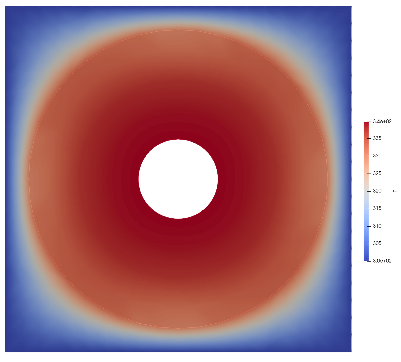
From solid_out.e and solid_out_fluid0.e in Paraview, last timestep