Phase 2: Time-dependent Multiphysics Coupling
Description
This phase is composed of a sole task which aims to verify the multiphysics coupled transient calculations. The heat transfer coefficient is represented by a sinusoidal function of the following form (1) where is the reference volumetric heat transfer coefficient, and f is the frequency which results in a sinusoidal behavior of the reactor power. In the simulation, varying values of frequency used are 0.0125, 0.025, 0.05, 0.1, 0.2, 0.4, 0.8. The power gain in the reactor with the varying power can be calculated as a function of frequency according to the following equation
There are two coupled inputs for this stage. The first performs the neutronics calculations and the second performs the Navier-Stocks solution. The sinusoidal power behavior modeling is defined in the neutronics input as a function within the Functions
[Functions]
  [alpha_val]
    type = ParsedFunction
    expression = '1.0e+6*(1.0 + 0.1*sin(2.0*pi*${frequency}*t))' #  'alpha_0*(1.0 + a*sin(fq*t))'
  []
[]
(msr/cnrs/s21/cnrs_s21_ns_flow.i)For each frequency, 10 cycles are ran to obtain the asymptotic power wave. The last three cycles are used to obtain the power gain and phase shift. The problem is set to transient and the time step size is set inversely proportional to the frequency. This is requested in the Executioner
[Executioner]
  type = Transient
  solve_type = PJFNK
  petsc_options_iname = '-pc_type -pc_factor_shift_type -pc_factor_mat_solver_package'
  petsc_options_value = 'lu NONZERO superlu_dist'

  start_time = 0.0
  dt = '${fparse max(0.005, 0.05*0.0125/frequency)}'
  end_time = '${fparse 10/frequency}'
  #[TimeStepper]
  #  type = IterationAdaptiveDT
  #  dt = 0.1
  #  growth_factor = 2
  #[]
  line_search = none #l2
  l_max_its = 200
  l_tol = 1e-3
  nl_max_its = 200
  nl_rel_tol = 1e-6
  nl_abs_tol = 1e-8

  # MultiApp iteration parameters
  fixed_point_min_its = 2
  fixed_point_max_its = 50
  fixed_point_rel_tol = 1e-6
  fixed_point_abs_tol = 1e-6
[]
(msr/cnrs/s21/cnrs_s21_griffin_neutronics.i)The rest of the transport solve input has a structure similar to that of the transport input in Step 1.3. The difference is in assigning a transienteigenvaluetypeExecutionerTransient
On the Navier-Stokes solve side, the problem is still executed as a transient solver. However, instead of running the problem for a long time to achieve steady state, the problem is defined as follows
[Executioner]
  type = Transient
  start_time = 0.0
  dt = '${fparse max(0.005, 0.05*0.0125/frequency)}'
  end_time = '${fparse 10/frequency}'
  #[TimeStepper]
  #  type = IterationAdaptiveDT
  #  dt = 0.1
  #  growth_factor = 2
  #[]
  solve_type = 'NEWTON'
  petsc_options_iname = '-pc_type -pc_factor_shift_type -pc_factor_mat_solver_package'
  petsc_options_value = 'lu NONZERO superlu_dist'
  line_search = l2 #'none'
  nl_rel_tol = 1e-6
  nl_abs_tol = 2e-8
  nl_max_its = 200
  l_max_its = 200
  automatic_scaling = true
[]
(msr/cnrs/s21/cnrs_s21_ns_flow.i)Results
The results for this exercise report the power gain and the phase shift as a function of the frequency as defined above. The power gain decreases with increases the frequency, and the phase shift approaches 90 degrees with increasing the frequency. These results are displayed in Figure 1
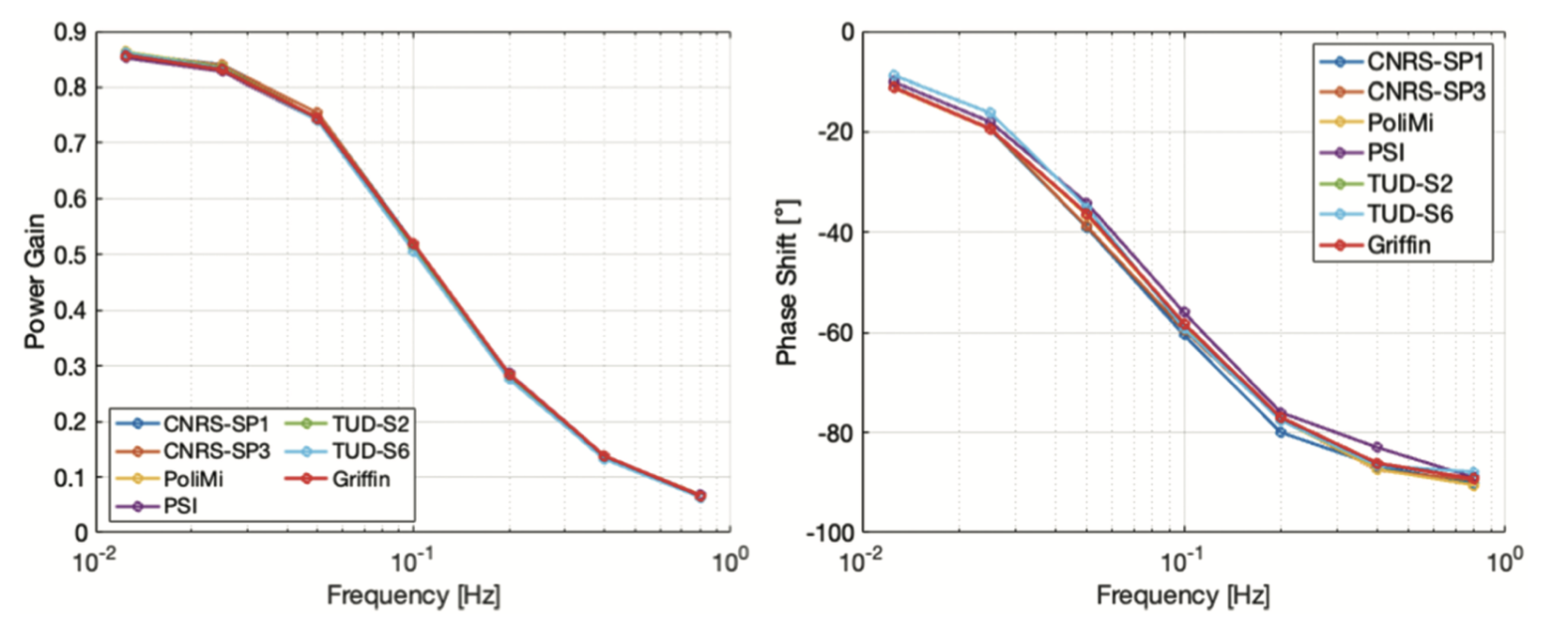
Figure 1:
(msr/cnrs/s21/cnrs_s21_ns_flow.i)
# ==============================================================================
# Model description
# ------------------------------------------------------------------------------
# CNRS Benchmark model Created & modifed by Dr. Mustafa Jaradat and Dr. Namjae Choi
# November 22, 2022
# Step 2.1: Time dependent coupling
# ==============================================================================
#   Tiberga, et al., 2020. Results from a multi-physics numerical benchmark for codes
#   dedicated to molten salt fast reactors. Ann. Nucl. Energy 142(2020)107428.
#   URL:http://www.sciencedirect.com/science/article/pii/S0306454920301262
# ==============================================================================

alpha = 2.0e-4
rho   = 2.0e+3
cp    = 3.075e+3
k     = 1.0e-3
mu    = 5.0e+1

# Sc_t =  2.0e8
Ulid = 0.5

lambda0 = 1.24667E-02
lambda1 = 2.82917E-02
lambda2 = 4.25244E-02
lambda3 = 1.33042E-01
lambda4 = 2.92467E-01
lambda5 = 6.66488E-01
lambda6 = 1.63478E+00
lambda7 = 3.55460E+00

beta0   =  2.33102e-4
beta1   =  1.03262e-3
beta2   =  6.81878e-4
beta3   =  1.37726e-3
beta4   =  2.14493e-3
beta5   =  6.40917e-4
beta6   =  6.05805e-4
beta7   =  1.66016e-4

frequency = 0.125

[Mesh]
  [fmg]
    type = FileMeshGenerator
    file = '../s14/cnrs_s14_griffin_neutronics_out_ns_flow0.e'
    use_for_exodus_restart = true
  []
[]


[Physics]
  [NavierStokes]
    [Flow]
      [all]
        compressibility = 'incompressible'
        density = ${rho}
        dynamic_viscosity = 'mu'

        # Restart parameters
        initialize_variables_from_mesh_file = true

        # Boussinesq parameters
        boussinesq_approximation = true
        gravity = '0 -9.81 0'
        thermal_expansion = ${alpha}
        ref_temperature = 900

        # Initial conditions
        initial_velocity = '${Ulid} 0 0'
        initial_pressure = 1e5

        # Boundary conditions
        # Note: we could do a no-slip with a wall velocity, same
        inlet_boundaries = 'top'
        momentum_inlet_types = 'fixed-velocity'
        momentum_inlet_functors = '${Ulid} 0'

        wall_boundaries = 'left right bottom'
        momentum_wall_types = 'noslip noslip noslip'

        # Pressure pin
        pin_pressure = true
        pinned_pressure_type = average
        pinned_pressure_value = 1e5

        # Numerical Scheme
        momentum_advection_interpolation = 'upwind'
        mass_advection_interpolation = 'upwind'
      []
    []
    [FluidHeatTransfer]
      [all]
        initial_temperature = 900

        # Restart parameters
        initialize_variables_from_mesh_file = true

        # Material properties
        thermal_conductivity = 'k'
        specific_heat = 'cp'

        # Boundary conditions
        energy_inlet_types = 'fixed-temperature'
        energy_inlet_functors = 900
        energy_wall_types = 'heatflux heatflux heatflux'
        energy_wall_functors = '0 0 0'

        # Heat source
        external_heat_source = power_density

        ambient_convection_alpha = 1.0e+6
        ambient_temperature = 900.0

        # Numerical Scheme
        energy_advection_interpolation = 'upwind'
        energy_two_term_bc_expansion = true
        energy_scaling = 1e-3
      []
    []
    [ScalarTransport]
      [scalars]
        # Restart parameters
        initialize_variables_from_mesh_file = true

        passive_scalar_names                = 'dnp0 dnp1 dnp2 dnp3
                                              dnp4 dnp5 dnp6 dnp7'
        passive_scalar_coupled_source       = 'fission_source dnp0; fission_source dnp1;
                                              fission_source dnp2; fission_source dnp3;
                                              fission_source dnp4; fission_source dnp5;
                                              fission_source dnp6; fission_source dnp7'
        passive_scalar_coupled_source_coeff = '${beta0} ${fparse -lambda0}; ${beta1} ${fparse -lambda1};
                                              ${beta2} ${fparse -lambda2}; ${beta3} ${fparse -lambda3};
                                              ${beta4} ${fparse -lambda4}; ${beta5} ${fparse -lambda5};
                                              ${beta6} ${fparse -lambda6}; ${beta7} ${fparse -lambda7}'
        passive_scalar_inlet_types          = 'fixed-value fixed-value fixed-value fixed-value
                                              fixed-value fixed-value fixed-value fixed-value'
        passive_scalar_inlet_functors       = '1.0; 1.0; 1.0; 1.0;
                                              1.0; 1.0; 1.0; 1.0'

        # Numerical parameters
        system_names= 's1 s2 s3 s4 s5 s6 s7 s8'
        passive_scalar_advection_interpolation = 'upwind'
      []
    []
  []
[]

[Problem]
  nl_sys_names = 'nl0 s1 s2 s3 s4 s5 s6 s7 s8'
[]

[AuxVariables]
  [power_density]
    type = MooseVariableFVReal
    initial_from_file_var = power_density
    initial_from_file_timestep = LATEST
  []
  [fission_source]
    type = MooseVariableFVReal
    initial_from_file_var = fission_source
    initial_from_file_timestep = LATEST
  []
[]

[Functions]
  [alpha_val]
     type = ParsedFunction
     expression = '1.0e+6*(1.0 + 0.1*sin(2.0*pi*${frequency}*t))' #  'alpha_0*(1.0 + a*sin(fq*t))'
  []
[]

[FunctorMaterials]
  [functor_constants]
    type = ADGenericFunctorMaterial
    prop_names = 'k rho mu'
    prop_values = '${k} ${rho} ${mu}'
  []
  [cp]
    type = ADGenericFunctorMaterial
    prop_names = 'cp'
    prop_values = '${cp}'
  []
  [alpha_t]
    type = ADGenericFunctorMaterial
    prop_names =  'alpha_t'
    prop_values = alpha_val
    block = '1'
  []
[]

[Debug]
  show_var_residual_norms = False
[]

[Postprocessors]
  [dt]
    type = TimestepSize
  []
  [Tfuel_avg]
    type = ElementAverageValue
    variable = T_fluid
  []
[]

[Executioner]
  type = Transient
  start_time = 0.0
  dt = ${fparse max(0.005, 0.05*0.0125/frequency)}
  end_time = ${fparse 10/frequency}
  #[TimeStepper]
  #  type = IterationAdaptiveDT
  #  dt = 0.1
  #  growth_factor = 2
  #[]
  solve_type = 'NEWTON'
  petsc_options_iname = '-pc_type -pc_factor_shift_type -pc_factor_mat_solver_package'
  petsc_options_value = 'lu NONZERO superlu_dist'
  line_search = l2#'none'
  nl_rel_tol = 1e-6
  nl_abs_tol = 2e-8
  nl_max_its = 200
  l_max_its = 200
  automatic_scaling = true
[]

[Outputs]
  exodus = false
  csv = true
  print_linear_converged_reason = false
  print_linear_residuals = false
  print_nonlinear_converged_reason = false
[]
(msr/cnrs/s21/cnrs_s21_griffin_neutronics.i)
# ==============================================================================
# Model description
# ------------------------------------------------------------------------------
# CNRS Benchmark model Created & modifed by Dr. Mustafa Jaradat and Dr. Namjae Choi
# November 22, 2022
# Step 2.1: Time dependent coupling
# ==============================================================================
#   Tiberga, et al., 2020. Results from a multi-physics numerical benchmark for codes
#   dedicated to molten salt fast reactors. Ann. Nucl. Energy 142(2020)107428.
#   URL:http://www.sciencedirect.com/science/article/pii/S0306454920301262
# ==============================================================================

frequency = 0.0125

[GlobalParams]
  isotopes = 'pseudo'
  densities = 'densityf'
  library_file = '../xs/msr_cavity_xslib.xml'
  library_name = 'CNRS-Benchmark'
  grid_names = 'Tfuel'
  grid_variables = 'tfuel'
  is_meter = true
  plus = 1
[]

[Mesh]
  type = MeshGeneratorMesh
  block_id = '1'
  block_name = 'cavity'
  [cartesian_mesh]
    type = CartesianMeshGenerator
    dim = 2
    dx = '1.0 1.0'
    ix = '100 100'
    dy = '1.0 1.0'
    iy = '100 100'
    subdomain_id = ' 1 1
                     1 1'
  []
  [assign_material_id]
    type = SubdomainExtraElementIDGenerator
    input = cartesian_mesh
    extra_element_id_names = 'material_id'
    subdomains = '1'
    extra_element_ids = '1'
  []
[]

[TransportSystems]
  particle = neutron
  equation_type = transient
  G = 6
  VacuumBoundary = 'left bottom right top'
  # Only for exodus restart, not SolutionFile restart
  # restart_transport_system = true
  [diff]
    scheme = CFEM-Diffusion
    n_delay_groups = 8
    family = LAGRANGE
    order = FIRST
    external_dnp_variable = 'dnp'
    fission_source_aux = true
    assemble_scattering_jacobian = true
    assemble_fission_jacobian = true
  []
[]

[PowerDensity]
  power = 1.0e9
  power_density_variable = power_density
  integrated_power_postprocessor = total_power
  family = LAGRANGE
  order = FIRST
[]

[AuxVariables]
  [tfuel]
    order = CONSTANT
    family = MONOMIAL
  []
  [tfuel_avg]
    order = CONSTANT
    family = MONOMIAL
  []
  [densityf]
    order = CONSTANT
    family = MONOMIAL
  []
  [dnp]
    order = CONSTANT
    family = MONOMIAL
    components = 8
  []
  [dnp0]
    order = CONSTANT
    family = MONOMIAL
  []
  [dnp1]
    order = CONSTANT
    family = MONOMIAL
  []
  [dnp2]
    order = CONSTANT
    family = MONOMIAL
  []
  [dnp3]
    order = CONSTANT
    family = MONOMIAL
  []
  [dnp4]
    order = CONSTANT
    family = MONOMIAL
  []
  [dnp5]
    order = CONSTANT
    family = MONOMIAL
  []
  [dnp6]
    order = CONSTANT
    family = MONOMIAL
  []
  [dnp7]
    order = CONSTANT
    family = MONOMIAL
  []
[]

[AuxKernels]
  [density_fuel]
    type = ParsedAux
    block = 'cavity'
    variable = densityf
    coupled_variables = 'tfuel'
    expression = '(1.0-0.0002*(tfuel-900.0))'
    execute_on = 'INITIAL timestep_end'
  []
  [build_dnp]
    type = BuildArrayVariableAux
    variable = dnp
    component_variables = 'dnp0 dnp1 dnp2 dnp3 dnp4 dnp5 dnp6 dnp7'
    execute_on = 'initial timestep_begin timestep_end'
  []
[]

[UserObjects]
  [transport_solution]
    type = TransportSolutionVectorFile
    transport_system = diff
    writing = false
    execute_on = 'INITIAL'
    scale_with_keff = false
    folder = '../s14'
  []
  [TH_solution]
    type = SolutionVectorFile
    var = 'tfuel densityf dnp0 dnp1 dnp2 dnp3 dnp4 dnp5 dnp6 dnp7'
    loading_var = 'tfuel densityf dnp0 dnp1 dnp2 dnp3 dnp4 dnp5 dnp6 dnp7'
    writing = false
    execute_on = 'INITIAL'
    folder = '../s14'
  []
[]

[Materials]
  [nm]
    type = CoupledFeedbackMatIDNeutronicsMaterial
    block = 'cavity'
  []
[]

[Preconditioning]
  [SMP]
    type = SMP
    full = true
  []
[]

[Executioner]
  type = Transient
  solve_type = PJFNK
  petsc_options_iname = '-pc_type -pc_factor_shift_type -pc_factor_mat_solver_package'
  petsc_options_value = 'lu NONZERO superlu_dist'

  start_time = 0.0
  dt = ${fparse max(0.005, 0.05*0.0125/frequency)}
  end_time = ${fparse 10/frequency}
  #[TimeStepper]
  #  type = IterationAdaptiveDT
  #  dt = 0.1
  #  growth_factor = 2
  #[]
  line_search = none #l2
  l_max_its = 200
  l_tol = 1e-3
  nl_max_its = 200
  nl_rel_tol = 1e-6
  nl_abs_tol = 1e-8

  # MultiApp iteration parameters
  fixed_point_min_its = 2
  fixed_point_max_its = 50
  fixed_point_rel_tol = 1e-6
  fixed_point_abs_tol = 1e-6
[]

[MultiApps]
  [ns_flow]
    type = TransientMultiApp
    input_files = cnrs_s21_ns_flow.i
    execute_on = 'timestep_end'
    keep_solution_during_restore = true
    catch_up = true
    cli_args = 'frequency=${frequency}'
  []
[]

[Transfers]
  # Multiphysics coupling
  # Send production terms
  [power_dens]
    type = MultiAppProjectionTransfer
    to_multi_app = ns_flow
    source_variable = 'power_density'
    variable = 'power_density'
    execute_on = 'timestep_end'
  []
  [fission_source]
    type = MultiAppProjectionTransfer
    to_multi_app = ns_flow
    source_variable = fission_source
    variable = fission_source
    execute_on = 'timestep_end'
  []

  # get quantities computed by the fluid flow caculation
  [fuel_temp]
    type = MultiAppCopyTransfer
    from_multi_app = ns_flow
    source_variable = 'T_fluid'
    variable = 'tfuel'
    execute_on = 'timestep_end'
  []
  [Tfuel_avg]
    type = MultiAppVariableValueSamplePostprocessorTransfer
    from_multi_app = ns_flow
    postprocessor = Tfuel_avg
    source_variable = 'tfuel_avg'
    execute_on = 'timestep_end'
  []
  [c1]
    type = MultiAppCopyTransfer
    from_multi_app = ns_flow
    source_variable = 'dnp0'
    variable = 'dnp0'
    execute_on = 'timestep_end'
  []
  [c2]
    type = MultiAppCopyTransfer
    from_multi_app = ns_flow
    source_variable = 'dnp1'
    variable = 'dnp1'
    execute_on = 'timestep_end'
  []
  [c3]
    type = MultiAppCopyTransfer
    from_multi_app = ns_flow
    source_variable = 'dnp2'
    variable = 'dnp2'
    execute_on = 'timestep_end'
  []
  [c4]
    type = MultiAppCopyTransfer
    from_multi_app = ns_flow
    source_variable = 'dnp3'
    variable = 'dnp3'
    execute_on = 'timestep_end'
  []
  [c5]
    type = MultiAppCopyTransfer
    from_multi_app = ns_flow
    source_variable = 'dnp4'
    variable = 'dnp4'
    execute_on = 'timestep_end'
  []
  [c6]
    type = MultiAppCopyTransfer
    from_multi_app = ns_flow
    source_variable = 'dnp5'
    variable = 'dnp5'
    execute_on = 'timestep_end'
  []
  [c7]
    type = MultiAppCopyTransfer
    from_multi_app = ns_flow
    source_variable = 'dnp6'
    variable = 'dnp6'
    execute_on = 'timestep_end'
  []
  [c8]
    type = MultiAppCopyTransfer
    from_multi_app = ns_flow
    source_variable = 'dnp7'
    variable = 'dnp7'
    execute_on = 'timestep_end'
  []
[]

[Postprocessors]
  [Tfuel_avg2]
    type = ElementAverageValue
    variable = tfuel
    execute_on = 'initial timestep_end'
  []
[]

[Outputs]
  exodus = true
  csv = true
  print_linear_converged_reason = false
  print_linear_residuals = false
  print_nonlinear_converged_reason = false
[]
(msr/cnrs/s21/cnrs_s21_ns_flow.i)
# ==============================================================================
# Model description
# ------------------------------------------------------------------------------
# CNRS Benchmark model Created & modifed by Dr. Mustafa Jaradat and Dr. Namjae Choi
# November 22, 2022
# Step 2.1: Time dependent coupling
# ==============================================================================
#   Tiberga, et al., 2020. Results from a multi-physics numerical benchmark for codes
#   dedicated to molten salt fast reactors. Ann. Nucl. Energy 142(2020)107428.
#   URL:http://www.sciencedirect.com/science/article/pii/S0306454920301262
# ==============================================================================

alpha = 2.0e-4
rho   = 2.0e+3
cp    = 3.075e+3
k     = 1.0e-3
mu    = 5.0e+1

# Sc_t =  2.0e8
Ulid = 0.5

lambda0 = 1.24667E-02
lambda1 = 2.82917E-02
lambda2 = 4.25244E-02
lambda3 = 1.33042E-01
lambda4 = 2.92467E-01
lambda5 = 6.66488E-01
lambda6 = 1.63478E+00
lambda7 = 3.55460E+00

beta0   =  2.33102e-4
beta1   =  1.03262e-3
beta2   =  6.81878e-4
beta3   =  1.37726e-3
beta4   =  2.14493e-3
beta5   =  6.40917e-4
beta6   =  6.05805e-4
beta7   =  1.66016e-4

frequency = 0.125

[Mesh]
  [fmg]
    type = FileMeshGenerator
    file = '../s14/cnrs_s14_griffin_neutronics_out_ns_flow0.e'
    use_for_exodus_restart = true
  []
[]


[Physics]
  [NavierStokes]
    [Flow]
      [all]
        compressibility = 'incompressible'
        density = ${rho}
        dynamic_viscosity = 'mu'

        # Restart parameters
        initialize_variables_from_mesh_file = true

        # Boussinesq parameters
        boussinesq_approximation = true
        gravity = '0 -9.81 0'
        thermal_expansion = ${alpha}
        ref_temperature = 900

        # Initial conditions
        initial_velocity = '${Ulid} 0 0'
        initial_pressure = 1e5

        # Boundary conditions
        # Note: we could do a no-slip with a wall velocity, same
        inlet_boundaries = 'top'
        momentum_inlet_types = 'fixed-velocity'
        momentum_inlet_functors = '${Ulid} 0'

        wall_boundaries = 'left right bottom'
        momentum_wall_types = 'noslip noslip noslip'

        # Pressure pin
        pin_pressure = true
        pinned_pressure_type = average
        pinned_pressure_value = 1e5

        # Numerical Scheme
        momentum_advection_interpolation = 'upwind'
        mass_advection_interpolation = 'upwind'
      []
    []
    [FluidHeatTransfer]
      [all]
        initial_temperature = 900

        # Restart parameters
        initialize_variables_from_mesh_file = true

        # Material properties
        thermal_conductivity = 'k'
        specific_heat = 'cp'

        # Boundary conditions
        energy_inlet_types = 'fixed-temperature'
        energy_inlet_functors = 900
        energy_wall_types = 'heatflux heatflux heatflux'
        energy_wall_functors = '0 0 0'

        # Heat source
        external_heat_source = power_density

        ambient_convection_alpha = 1.0e+6
        ambient_temperature = 900.0

        # Numerical Scheme
        energy_advection_interpolation = 'upwind'
        energy_two_term_bc_expansion = true
        energy_scaling = 1e-3
      []
    []
    [ScalarTransport]
      [scalars]
        # Restart parameters
        initialize_variables_from_mesh_file = true

        passive_scalar_names                = 'dnp0 dnp1 dnp2 dnp3
                                              dnp4 dnp5 dnp6 dnp7'
        passive_scalar_coupled_source       = 'fission_source dnp0; fission_source dnp1;
                                              fission_source dnp2; fission_source dnp3;
                                              fission_source dnp4; fission_source dnp5;
                                              fission_source dnp6; fission_source dnp7'
        passive_scalar_coupled_source_coeff = '${beta0} ${fparse -lambda0}; ${beta1} ${fparse -lambda1};
                                              ${beta2} ${fparse -lambda2}; ${beta3} ${fparse -lambda3};
                                              ${beta4} ${fparse -lambda4}; ${beta5} ${fparse -lambda5};
                                              ${beta6} ${fparse -lambda6}; ${beta7} ${fparse -lambda7}'
        passive_scalar_inlet_types          = 'fixed-value fixed-value fixed-value fixed-value
                                              fixed-value fixed-value fixed-value fixed-value'
        passive_scalar_inlet_functors       = '1.0; 1.0; 1.0; 1.0;
                                              1.0; 1.0; 1.0; 1.0'

        # Numerical parameters
        system_names= 's1 s2 s3 s4 s5 s6 s7 s8'
        passive_scalar_advection_interpolation = 'upwind'
      []
    []
  []
[]

[Problem]
  nl_sys_names = 'nl0 s1 s2 s3 s4 s5 s6 s7 s8'
[]

[AuxVariables]
  [power_density]
    type = MooseVariableFVReal
    initial_from_file_var = power_density
    initial_from_file_timestep = LATEST
  []
  [fission_source]
    type = MooseVariableFVReal
    initial_from_file_var = fission_source
    initial_from_file_timestep = LATEST
  []
[]

[Functions]
  [alpha_val]
     type = ParsedFunction
     expression = '1.0e+6*(1.0 + 0.1*sin(2.0*pi*${frequency}*t))' #  'alpha_0*(1.0 + a*sin(fq*t))'
  []
[]

[FunctorMaterials]
  [functor_constants]
    type = ADGenericFunctorMaterial
    prop_names = 'k rho mu'
    prop_values = '${k} ${rho} ${mu}'
  []
  [cp]
    type = ADGenericFunctorMaterial
    prop_names = 'cp'
    prop_values = '${cp}'
  []
  [alpha_t]
    type = ADGenericFunctorMaterial
    prop_names =  'alpha_t'
    prop_values = alpha_val
    block = '1'
  []
[]

[Debug]
  show_var_residual_norms = False
[]

[Postprocessors]
  [dt]
    type = TimestepSize
  []
  [Tfuel_avg]
    type = ElementAverageValue
    variable = T_fluid
  []
[]

[Executioner]
  type = Transient
  start_time = 0.0
  dt = ${fparse max(0.005, 0.05*0.0125/frequency)}
  end_time = ${fparse 10/frequency}
  #[TimeStepper]
  #  type = IterationAdaptiveDT
  #  dt = 0.1
  #  growth_factor = 2
  #[]
  solve_type = 'NEWTON'
  petsc_options_iname = '-pc_type -pc_factor_shift_type -pc_factor_mat_solver_package'
  petsc_options_value = 'lu NONZERO superlu_dist'
  line_search = l2#'none'
  nl_rel_tol = 1e-6
  nl_abs_tol = 2e-8
  nl_max_its = 200
  l_max_its = 200
  automatic_scaling = true
[]

[Outputs]
  exodus = false
  csv = true
  print_linear_converged_reason = false
  print_linear_residuals = false
  print_nonlinear_converged_reason = false
[]