Phase 1 Model: Steady State MultiPhysics Coupling
This phase of the benchmark is concerned with the steady state multiphysics solution. It is comprised of four steps and following is a description of the four steps and their inputs.
Step 1.1
In this step, the influence of the delayed neutron precursor drift on the reactivity and delayed neutron source distribution is explored. This step comprises a neutronic and Navier-Stokes solves. The neutronics solve is performed as a diffusion problem as defined in step 0.2. The main input file contains instructions to perform a neutronic solution. The characteristics of the transport solve are defined TransportSystems block as follows
[TransportSystems]
  particle = neutron
  equation_type = eigenvalue
  G = 6
  VacuumBoundary = 'left bottom right top'
  [diff]
    scheme = CFEM-Diffusion
    n_delay_groups = 8
    family = LAGRANGE
    order = FIRST
    external_dnp_variable = 'dnp'
    fission_source_aux = true
    assemble_scattering_jacobian = true
    assemble_fission_jacobian = true
  []
[]The power of the problem from which the power density will be normalized can be defined in the PowerDensity block as follows
[PowerDensity]
  power = 1.0e9
  power_density_variable = power_density
  integrated_power_postprocessor = total_power
  power_scaling_postprocessor = Normalization
  family = LAGRANGE
  order = FIRST
[]auxiliary variables for the problem are defined in the AuxVariables block as follows
[AuxVariables]
  [tfuel]
    order = CONSTANT
    family = MONOMIAL
    initial_condition = 900
  []
  [tfuel_avg]
    order = CONSTANT
    family = MONOMIAL
    initial_condition = 900
  []
  [densityf]
    order = CONSTANT
    family = MONOMIAL
    initial_condition = 1.0
  []
  [dnp_src]
    order = CONSTANT
    family = MONOMIAL
  []
  [dnp]
    order = CONSTANT
    family = MONOMIAL
    components = 8
  []
  [dnp0]
    order = CONSTANT
    family = MONOMIAL
  []
  [dnp1]
    order = CONSTANT
    family = MONOMIAL
  []
  [dnp2]
    order = CONSTANT
    family = MONOMIAL
  []
  [dnp3]
    order = CONSTANT
    family = MONOMIAL
  []
  [dnp4]
    order = CONSTANT
    family = MONOMIAL
  []
  [dnp5]
    order = CONSTANT
    family = MONOMIAL
  []
  [dnp6]
    order = CONSTANT
    family = MONOMIAL
  []
  [dnp7]
    order = CONSTANT
    family = MONOMIAL
  []
[]where pronghorn will be used to obtain the temperature distributions and the delayed neutron precursor distributions. Operations to act on the auxiliary variables are defined in the AuxKernels block
[AuxKernels]
  [density_fuel]
    type = ParsedAux
    block = 'cavity'
    variable = densityf
    coupled_variables = 'tfuel'
    expression = '(1.0-0.0002*(tfuel-900.0))'
    execute_on = 'INITIAL timestep_end'
  []
  [build_dnp]
    type = BuildArrayVariableAux
    variable = dnp
    component_variables = 'dnp0 dnp1 dnp2 dnp3 dnp4 dnp5 dnp6 dnp7'
    execute_on = 'initial timestep_begin final'
  []
  [delayed_neutron_source]
    type = VectorReactionRate
    scalar_flux = 'dnp0 dnp1 dnp2 dnp3 dnp4 dnp5 dnp6 dnp7'
    cross_section = lambda_vec
    variable = dnp_src
    scale_factor = Normalization
    block = '1'
  []
[]The characteristics of executing the calculations are provided in the Executioner block as follows
[Executioner]
  type = Eigenvalue
  solve_type = PJFNK
  petsc_options_iname = '-pc_type -pc_factor_shift_type -pc_factor_mat_solver_package'
  petsc_options_value = 'lu NONZERO superlu_dist'
  free_power_iterations = 2
  line_search = none #l2
  l_max_its = 200
  l_tol = 1e-3
  nl_max_its = 200
  nl_rel_tol = 1e-5
  nl_abs_tol = 1e-6
  fixed_point_min_its = 3
  fixed_point_max_its = 50
  fixed_point_rel_tol = 1e-5
  fixed_point_abs_tol = 1e-6
[]To obtain the temperature and delayed neutron precursor distribution, pronghorn is used to performed these thermo-fluid calculations. A MultiApps block is used to call the pronghorn solver as in the following block of code
[MultiApps]
  [ns_flow]
    type = FullSolveMultiApp
    input_files = cnrs_s11_ns_flow.i
    execute_on = 'TIMESTEP_END'
  []
[]where ''cnrs_s01_ns_flow.i'' is the pronghorn input. The transfer of variables between Griffin and pronghorn is instructed through the Transfers block, where the fission source is obtained using Griffin and sent to pronghorn. Then pronghorn is used to calculate the distribution of the precursor
[Transfers]
  [fission_source]
    type = MultiAppProjectionTransfer
    to_multi_app = ns_flow
    source_variable = fission_source
    variable = fission_source
    execute_on = 'timestep_end'
  []
  [c1]
    type = MultiAppCopyTransfer
    from_multi_app = ns_flow
    source_variable = 'dnp0'
    variable = 'dnp0'
    execute_on = 'timestep_end'
  []
  [c2]
    type = MultiAppCopyTransfer
    from_multi_app = ns_flow
    source_variable = 'dnp1'
    variable = 'dnp1'
    execute_on = 'timestep_end'
  []
  [c3]
    type = MultiAppCopyTransfer
    from_multi_app = ns_flow
    source_variable = 'dnp2'
    variable = 'dnp2'
    execute_on = 'timestep_end'
  []
  [c4]
    type = MultiAppCopyTransfer
    from_multi_app = ns_flow
    source_variable = 'dnp3'
    variable = 'dnp3'
    execute_on = 'timestep_end'
  []
  [c5]
    type = MultiAppCopyTransfer
    from_multi_app = ns_flow
    source_variable = 'dnp4'
    variable = 'dnp4'
    execute_on = 'timestep_end'
  []
  [c6]
    type = MultiAppCopyTransfer
    from_multi_app = ns_flow
    source_variable = 'dnp5'
    variable = 'dnp5'
    execute_on = 'timestep_end'
  []
  [c7]
    type = MultiAppCopyTransfer
    from_multi_app = ns_flow
    source_variable = 'dnp6'
    variable = 'dnp6'
    execute_on = 'timestep_end'
  []
  [c8]
    type = MultiAppCopyTransfer
    from_multi_app = ns_flow
    source_variable = 'dnp7'
    variable = 'dnp7'
    execute_on = 'timestep_end'
  []
[]The pronghorn input to obtain the delayed neutron precursor distribution and fuel temperature is similar in structure to the input developed in step 0.1. Some differences in the input file for the Navier-Stokes solve include modifying the input to include introducing the fission_source as an auxiliary variable that pronghorn will expect to receive from the Griffin Solve.
[AuxVariables]
  [tfuel]
    order = CONSTANT
    family = MONOMIAL
    initial_condition = 900
  []
  [tfuel_avg]
    order = CONSTANT
    family = MONOMIAL
    initial_condition = 900
  []
  [densityf]
    order = CONSTANT
    family = MONOMIAL
    initial_condition = 1.0
  []
  [dnp_src]
    order = CONSTANT
    family = MONOMIAL
  []
  [dnp]
    order = CONSTANT
    family = MONOMIAL
    components = 8
  []
  [dnp0]
    order = CONSTANT
    family = MONOMIAL
  []
  [dnp1]
    order = CONSTANT
    family = MONOMIAL
  []
  [dnp2]
    order = CONSTANT
    family = MONOMIAL
  []
  [dnp3]
    order = CONSTANT
    family = MONOMIAL
  []
  [dnp4]
    order = CONSTANT
    family = MONOMIAL
  []
  [dnp5]
    order = CONSTANT
    family = MONOMIAL
  []
  [dnp6]
    order = CONSTANT
    family = MONOMIAL
  []
  [dnp7]
    order = CONSTANT
    family = MONOMIAL
  []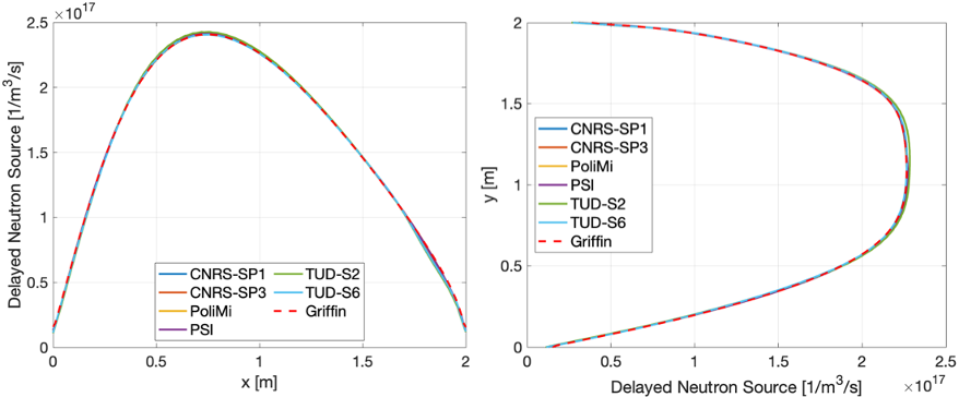
[]Step 1.1 Results
The delayed neutron source distribution along AA` and BB` are collected from the results of the Griffin run. These are as follows
Step 1.2
This step resembles step 1.1 with the difference being in introducing the temperature feedback. The problem is treated as a transport solve coupled with two Navier-Stokes solves as will be described later. The transport solve is specified in the TransportSystems block as follows
[TransportSystems]
  particle = neutron
  equation_type = eigenvalue
  G = 6
  VacuumBoundary = 'left bottom right top'
  [diff]
    scheme = CFEM-Diffusion
    n_delay_groups = 8
    family = LAGRANGE
    order = FIRST
    external_dnp_variable = 'dnp'
    fission_source_aux = true
    assemble_scattering_jacobian = true
    assemble_fission_jacobian = true
  []
[]The power density in the fuel salt normalization given a reactor power is instructed in the PowerDensity as follows
[PowerDensity]
  power = 1.0e9
  power_density_variable = power_density
  integrated_power_postprocessor = total_power
  power_scaling_postprocessor = Normalization
  family = LAGRANGE
  order = FIRST
[]A set of auxiliary variables which will be obtained using other applications (i.e. pronghorn) are defined as follows. These variables include the temperature distributions in the fuel, flow field, and delayed neutron precursor distribution which are obtained using Navier-Stokes solves as will be demonstrated later.
[AuxVariables]
  [tfuel]
    order = CONSTANT
    family = MONOMIAL
    initial_condition = 900
  []
  [tfuel_avg]
    order = CONSTANT
    family = MONOMIAL
    initial_condition = 900
  []
  [vel_x]
    order = CONSTANT
    family = MONOMIAL
  []
  [vel_y]
    order = CONSTANT
    family = MONOMIAL
  []
  [densityf]
    order = CONSTANT
    family = MONOMIAL
    initial_condition = 1.0
  []
  [FRD]
    order = FIRST
    family = L2_LAGRANGE
  []
  [dnp]
    order = CONSTANT
    family = MONOMIAL
    components = 8
  []
  [dnp0]
    order = CONSTANT
    family = MONOMIAL
  []
  [dnp1]
    order = CONSTANT
    family = MONOMIAL
  []
  [dnp2]
    order = CONSTANT
    family = MONOMIAL
  []
  [dnp3]
    order = CONSTANT
    family = MONOMIAL
  []
  [dnp4]
    order = CONSTANT
    family = MONOMIAL
  []
  [dnp5]
    order = CONSTANT
    family = MONOMIAL
  []
  [dnp6]
    order = CONSTANT
    family = MONOMIAL
  []
  [dnp7]
    order = CONSTANT
    family = MONOMIAL
  []
[]Compared to the previous step (i.e. Step 1.1), there will be two pronghorn Navier-Stokes solutions to apply the temperature feedback. These are called in a MultiApps fashion as
[MultiApps]
  [ns_flow]
    type = FullSolveMultiApp
    input_files = cnrs_s12_ns_flow.i
    execute_on = 'TIMESTEP_END'
  []
[]The first solve (i.e. ns_flow) will be used to solve for the flow field (i.e. velocity field) and the delayed neutron precursor distribution. The input for the first solve will be the fission_source obtained by the Griffin transport solve. The second solve (i.e. ns_temp) is used to solve for the temperature distribution given the fission source solution obtained by the transport solve. The inputs for the second solve are velocity field obtained by the ns_flow solve, and the power density obtained by the Griffin transport solve. The instructions of data transfer between the transport solve and the two Navier-Stokes solves are provided in the Transfers block as follows
[Transfers]
  # MultiPhysics coupling
  [fission_source]
    type = MultiAppProjectionTransfer
    to_multi_app = ns_flow
    source_variable = fission_source
    variable = fission_source
    execute_on = 'TIMESTEP_BEGIN'
  []
  [power_dens]
    type = MultiAppProjectionTransfer
    to_multi_app = ns_flow
    source_variable = 'power_density'
    variable = 'power_density'
    execute_on = 'TIMESTEP_END'
  []

  # Computed in the flow simulation
  [c1]
    type = MultiAppCopyTransfer
    from_multi_app = ns_flow
    source_variable = 'dnp0'
    variable = 'dnp0'
    execute_on = 'TIMESTEP_END'
  []
  [c2]
    type = MultiAppCopyTransfer
    from_multi_app = ns_flow
    source_variable = 'dnp1'
    variable = 'dnp1'
    execute_on = 'TIMESTEP_END'
  []
  [c3]
    type = MultiAppCopyTransfer
    from_multi_app = ns_flow
    source_variable = 'dnp2'
    variable = 'dnp2'
    execute_on = 'TIMESTEP_END'
  []
  [c4]
    type = MultiAppCopyTransfer
    from_multi_app = ns_flow
    source_variable = 'dnp3'
    variable = 'dnp3'
    execute_on = 'TIMESTEP_END'
  []
  [c5]
    type = MultiAppCopyTransfer
    from_multi_app = ns_flow
    source_variable = 'dnp4'
    variable = 'dnp4'
    execute_on = 'TIMESTEP_END'
  []
  [c6]
    type = MultiAppCopyTransfer
    from_multi_app = ns_flow
    source_variable = 'dnp5'
    variable = 'dnp5'
    execute_on = 'TIMESTEP_END'
  []
  [c7]
    type = MultiAppCopyTransfer
    from_multi_app = ns_flow
    source_variable = 'dnp6'
    variable = 'dnp6'
    execute_on = 'TIMESTEP_END'
  []
  [c8]
    type = MultiAppCopyTransfer
    from_multi_app = ns_flow
    source_variable = 'dnp7'
    variable = 'dnp7'
    execute_on = 'TIMESTEP_END'
  []
  [fuel_temp]
    type = MultiAppCopyTransfer
    from_multi_app = ns_flow
    source_variable = 'T_fluid'
    variable = 'tfuel'
    execute_on = 'TIMESTEP_END'
  []
[]Te sequence of TransportSystems solve, ns_flow solve, and ns_temp solve is performed till the convergence criteria is met. These are specified in the main input file (i.e. Griffin solve), within the Executioner block as follows
[Executioner]
  type = Eigenvalue
  solve_type = PJFNK
  petsc_options_iname = '-pc_type -pc_factor_shift_type -pc_factor_mat_solver_package'
  petsc_options_value = 'lu NONZERO superlu_dist'
  free_power_iterations = 2
  line_search = none #l2
  l_max_its = 200
  l_tol = 1e-3
  nl_max_its = 200
  nl_rel_tol = 1e-5
  nl_abs_tol = 1e-6
  fixed_point_min_its = 3
  fixed_point_max_its = 50
  fixed_point_rel_tol = 1e-5
  fixed_point_abs_tol = 1e-6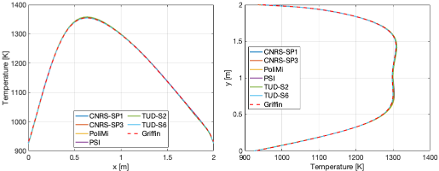
[]Step 1.2 Results
The fuel salt temperature distribution along AA` and BB` is collected and plotted as follows
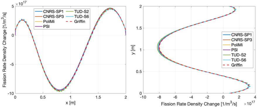
The fission rate density is also reported along AA` and BB` in this exercise
Step 1.3:
In this step, the coupled multiphysics modeling is performed with zero fuel salt lid velocity. This means the flow is only driven by natural circulation and without forced convection.
The modeling of this problem takes two solvers. The first is a transport solve specified through the TransportSystems block
[TransportSystems]
  particle = neutron
  equation_type = eigenvalue
  G = 6
  VacuumBoundary = 'left bottom right top'
  [diff]
    scheme = CFEM-Diffusion
    n_delay_groups = 8
    family = LAGRANGE
    order = FIRST
    external_dnp_variable = 'dnp'
    fission_source_aux = true
    assemble_scattering_jacobian = true
    assemble_fission_jacobian = true
  []
[]Power density instructions are provided in the PowerDensity block
[PowerDensity]
  power = 1.0e9
  power_density_variable = power_density
  integrated_power_postprocessor = total_power
  power_scaling_postprocessor = Normalization
  family = LAGRANGE
  order = FIRST
[]The set of auxiliary variables that will be obtained using the Navier-Stokes solves are defined as follows
[AuxVariables]
  [tfuel]
    order = CONSTANT
    family = MONOMIAL
    initial_condition = 900
  []
  [tfuel_avg]
    order = CONSTANT
    family = MONOMIAL
    initial_condition = 900
  []
  [vel_x]
    order = CONSTANT
    family = MONOMIAL
  []
  [vel_y]
    order = CONSTANT
    family = MONOMIAL
  []
  [densityf]
    order = CONSTANT
    family = MONOMIAL
    initial_condition = 1.0
  []
  [dnp_src]
    order = CONSTANT
    family = MONOMIAL
  []
  [dnp]
    order = CONSTANT
    family = MONOMIAL
    components = 8
  []
  [dnp0]
    order = CONSTANT
    family = MONOMIAL
  []
  [dnp1]
    order = CONSTANT
    family = MONOMIAL
  []
  [dnp2]
    order = CONSTANT
    family = MONOMIAL
  []
  [dnp3]
    order = CONSTANT
    family = MONOMIAL
  []
  [dnp4]
    order = CONSTANT
    family = MONOMIAL
  []
  [dnp5]
    order = CONSTANT
    family = MONOMIAL
  []
  [dnp6]
    order = CONSTANT
    family = MONOMIAL
  []
  [dnp7]
    order = CONSTANT
    family = MONOMIAL
  []
[]The transport solve characteristics and the tolerances to converge the problem are specified as follows
[Executioner]
  type = Eigenvalue
  solve_type = PJFNKMO
  petsc_options_iname = '-pc_type -pc_factor_shift_type -pc_factor_mat_solver_package'
  petsc_options_value = 'lu NONZERO superlu_dist'
  free_power_iterations = 2
  l_max_its = 200
  l_tol = 1e-3

  # Nonlinear solve
  nl_max_its = 200
  nl_rel_tol = 1e-5
  nl_abs_tol = 1e-6
  line_search = none #l2

  # MultiApps fixed point iterations
  fixed_point_min_its = 3
  fixed_point_max_its = 50
  fixed_point_rel_tol = 1e-5
  fixed_point_abs_tol = 1e-6
[]The Navier-Stokes solve input is specified through the MultiApps block as
[MultiApps]
  [ns_flow]
    type = FullSolveMultiApp
    input_files = cnrs_s13_ns_flow.i
    execute_on = 'timestep_end'
  []
[]Then the data transfer between the transport solve and the Navier-Stokes solve are managed through the Transfers block
[Transfers]
  # Multiphysics coupling
  # Send production terms
  [power_dens]
    type = MultiAppProjectionTransfer
    to_multi_app = ns_flow
    source_variable = 'power_density'
    variable = 'power_density'
    execute_on = 'timestep_end'
  []
  [fission_source]
    type = MultiAppProjectionTransfer
    to_multi_app = ns_flow
    source_variable = fission_source
    variable = fission_source
    execute_on = 'timestep_end'
  []

  # get quantities computed by the fluid flow caculation
  [fuel_temp]
    type = MultiAppCopyTransfer
    from_multi_app = ns_flow
    source_variable = 'T_fluid'
    variable = 'tfuel'
    execute_on = 'timestep_end'
  []
  [c1]
    type = MultiAppCopyTransfer
    from_multi_app = ns_flow
    source_variable = 'dnp0'
    variable = 'dnp0'
    execute_on = 'timestep_end'
  []
  [c2]
    type = MultiAppCopyTransfer
    from_multi_app = ns_flow
    source_variable = 'dnp1'
    variable = 'dnp1'
    execute_on = 'timestep_end'
  []
  [c3]
    type = MultiAppCopyTransfer
    from_multi_app = ns_flow
    source_variable = 'dnp2'
    variable = 'dnp2'
    execute_on = 'timestep_end'
  []
  [c4]
    type = MultiAppCopyTransfer
    from_multi_app = ns_flow
    source_variable = 'dnp3'
    variable = 'dnp3'
    execute_on = 'timestep_end'
  []
  [c5]
    type = MultiAppCopyTransfer
    from_multi_app = ns_flow
    source_variable = 'dnp4'
    variable = 'dnp4'
    execute_on = 'timestep_end'
  []
  [c6]
    type = MultiAppCopyTransfer
    from_multi_app = ns_flow
    source_variable = 'dnp5'
    variable = 'dnp5'
    execute_on = 'timestep_end'
  []
  [c7]
    type = MultiAppCopyTransfer
    from_multi_app = ns_flow
    source_variable = 'dnp6'
    variable = 'dnp6'
    execute_on = 'timestep_end'
  []
  [c8]
    type = MultiAppCopyTransfer
    from_multi_app = ns_flow
    source_variable = 'dnp7'
    variable = 'dnp7'
    execute_on = 'timestep_end'
  []

  # For postprocessing purposes
  [Tfuel_avg]
    type = MultiAppVariableValueSamplePostprocessorTransfer
    from_multi_app = ns_flow
    source_variable = 'tfuel_avg'
    postprocessor = Tfuel_avg
    execute_on = 'timestep_end'
  []
  [vel_x_comp]
    type = MultiAppCopyTransfer
    from_multi_app = ns_flow
    source_variable = 'vel_x'
    variable = 'vel_x'
    execute_on = 'TIMESTEP_END'
  []
  [vel_y_comp]
    type = MultiAppCopyTransfer
    from_multi_app = ns_flow
    source_variable = 'vel_y'
    variable = 'vel_y'
    execute_on = 'TIMESTEP_END'
  []
[]Step 1.3 Results
The horizontal velocity component distribution along AA` is reported in Figure 1.
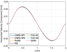
Figure 1:
The vertical velocity component distribution along AA` and BB` is also reported in Figure 2.
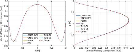
Figure 2:
The fuel salt temperature distribution along AA` and BB` in this exercise is reported in Figure 3.
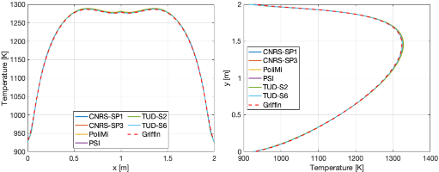
Figure 3:
Finally, the delayed neutron source distribution along AA` and BB` is reported in Figure 4.
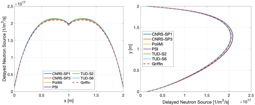
Figure 4:
Step 1.4:
This phase performs a similar task to that of Step 1.3 for a combination of reactor power and lid velocities. The set of reactor powers and lid velocities are presented in the following table
| Lid Velocity | Reactor Power |
|---|---|
| 0.0 | 1.0E9 |
| 0.1 | 0.2E9 |
| 0.1 | 0.4E9 |
| 0.1 | 0.6E9 |
| 0.1 | 0.8E9 |
| 0.1 | 1.0E9 |
| 0.2 | 0.2E9 |
| 0.2 | 0.4E9 |
| 0.2 | 0.6E9 |
| 0.2 | 0.8E9 |
| 0.2 | 1.0E9 |
| 0.3 | 0.2E9 |
| 0.3 | 0.4E9 |
| 0.3 | 0.6E9 |
| 0.3 | 0.8E9 |
| 0.3 | 1.0E9 |
| 0.4 | 0.2E9 |
| 0.4 | 0.4E9 |
| 0.4 | 0.6E9 |
| 0.4 | 0.8E9 |
| 0.4 | 1.0E9 |
| 0.5 | 0.2E9 |
| 0.5 | 0.4E9 |
| 0.5 | 0.6E9 |
| 0.5 | 0.8E9 |
| 0.5 | 1.0E9 |
A shell script is used to run all these cases.
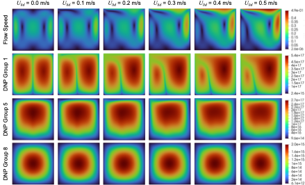
Step 1.4 Results
In this exercise, the reported results are the delayed neutron precursor density distribution depending on the lid velocity
(msr/cnrs/s11/cnrs_s11_griffin_neutronics.i)
# ==============================================================================
# Model description
# ------------------------------------------------------------------------------
# CNRS Benchmark model Created & modifed by Dr. Mustafa Jaradat and Dr. Namjae Choi
# November 22, 2022
# Step 1.1: Circulating fuel
# ==============================================================================
#   Tiberga, et al., 2020. Results from a multi-physics numerical benchmark for codes
#   dedicated to molten salt fast reactors. Ann. Nucl. Energy 142(2020)107428.
#   URL:http://www.sciencedirect.com/science/article/pii/S0306454920301262
# ==============================================================================

[GlobalParams]
  isotopes = 'pseudo'
  densities = 'densityf'
  library_file = '../xs/msr_cavity_xslib.xml'
  library_name = 'CNRS-Benchmark'
  grid_names = 'Tfuel'
  grid_variables = 'tfuel'
  is_meter = true
  plus = 1
[]
[Mesh]
  type = MeshGeneratorMesh
  block_id = '1'
  block_name = 'cavity'
  [cartesian_mesh]
    type = CartesianMeshGenerator
    dim = 2
    dx = '1.0 1.0'
    ix = '100 100'
    dy = '1.0 1.0'
    iy = '100 100'
    subdomain_id = ' 1 1
                     1 1'
  []
  [assign_material_id]
    type = SubdomainExtraElementIDGenerator
    input = cartesian_mesh
    extra_element_id_names = 'material_id'
    subdomains = '1'
    extra_element_ids = '1'
  []
[]

[TransportSystems]
  particle = neutron
  equation_type = eigenvalue
  G = 6
  VacuumBoundary = 'left bottom right top'
  [diff]
    scheme = CFEM-Diffusion
    n_delay_groups = 8
    family = LAGRANGE
    order = FIRST
    external_dnp_variable = 'dnp'
    fission_source_aux = true
    assemble_scattering_jacobian = true
    assemble_fission_jacobian = true
  []
[]

[PowerDensity]
  power = 1.0e9
  power_density_variable = power_density
  integrated_power_postprocessor = total_power
  power_scaling_postprocessor = Normalization
  family = LAGRANGE
  order = FIRST
[]

[AuxVariables]
  [tfuel]
    order = CONSTANT
    family = MONOMIAL
    initial_condition = 900
  []
  [tfuel_avg]
    order = CONSTANT
    family = MONOMIAL
    initial_condition = 900
  []
  [densityf]
    order = CONSTANT
    family = MONOMIAL
    initial_condition = 1.0
  []
  [dnp_src]
    order = CONSTANT
    family = MONOMIAL
  []
  [dnp]
    order = CONSTANT
    family = MONOMIAL
    components = 8
  []
  [dnp0]
    order = CONSTANT
    family = MONOMIAL
  []
  [dnp1]
    order = CONSTANT
    family = MONOMIAL
  []
  [dnp2]
    order = CONSTANT
    family = MONOMIAL
  []
  [dnp3]
    order = CONSTANT
    family = MONOMIAL
  []
  [dnp4]
    order = CONSTANT
    family = MONOMIAL
  []
  [dnp5]
    order = CONSTANT
    family = MONOMIAL
  []
  [dnp6]
    order = CONSTANT
    family = MONOMIAL
  []
  [dnp7]
    order = CONSTANT
    family = MONOMIAL
  []
[]

[AuxKernels]
  [density_fuel]
    type = ParsedAux
    block = 'cavity'
    variable = densityf
    coupled_variables = 'tfuel'
    expression = '(1.0-0.0002*(tfuel-900.0))'
    execute_on = 'INITIAL timestep_end'
  []
  [build_dnp]
    type = BuildArrayVariableAux
    variable = dnp
    component_variables = 'dnp0 dnp1 dnp2 dnp3 dnp4 dnp5 dnp6 dnp7'
    execute_on = 'initial timestep_begin final'
  []
  [delayed_neutron_source]
    type = VectorReactionRate
    scalar_flux = 'dnp0 dnp1 dnp2 dnp3 dnp4 dnp5 dnp6 dnp7'
    cross_section = lambda_vec
    variable = dnp_src
    scale_factor = Normalization
    block = '1'
  []
[]

[Materials]
  [fuel_salt]
    type = CoupledFeedbackMatIDNeutronicsMaterial
    block = 'cavity'
  []
[]

[Preconditioning]
  [SMP]
    type = SMP
    full = true
  []
[]

[Executioner]
  type = Eigenvalue
  solve_type = PJFNK
  petsc_options_iname = '-pc_type -pc_factor_shift_type -pc_factor_mat_solver_package'
  petsc_options_value = 'lu NONZERO superlu_dist'
  free_power_iterations = 2
  line_search = none #l2
  l_max_its = 200
  l_tol = 1e-3
  nl_max_its = 200
  nl_rel_tol = 1e-5
  nl_abs_tol = 1e-6
  fixed_point_min_its = 3
  fixed_point_max_its = 50
  fixed_point_rel_tol = 1e-5
  fixed_point_abs_tol = 1e-6
[]

[VectorPostprocessors]
  [AA_line_values_left]
    type = LineValueSampler
    start_point = '0 0.995 0'
    end_point = '2 0.995 0'
    variable = 'dnp_src'
    num_points = 201
    execute_on = 'FINAL'
    sort_by = x
  []
  [AA_line_values_right]
    type = LineValueSampler
    start_point = '0 1.005 0'
    end_point = '2 1.005 0'
    variable = 'dnp_src'
    num_points = 201
    execute_on = 'FINAL'
    sort_by = x
  []
  [BB_line_values_left]
    type = LineValueSampler
    start_point = '0.995 0 0'
    end_point = '0.995 2 0'
    variable = 'dnp_src'
    num_points = 201
    execute_on = 'FINAL'
    sort_by = y
  []
  [BB_line_values_right]
    type = LineValueSampler
    start_point = '1.005 0 0'
    end_point = '1.005 2 0'
    variable = 'dnp_src'
    num_points = 201
    execute_on = 'FINAL'
    sort_by = y
  []
[]

[MultiApps]
  [ns_flow]
    type = FullSolveMultiApp
    input_files = cnrs_s11_ns_flow.i
    execute_on = 'TIMESTEP_END'
  []
[]

[Transfers]
  [fission_source]
    type = MultiAppProjectionTransfer
    to_multi_app = ns_flow
    source_variable = fission_source
    variable = fission_source
    execute_on = 'timestep_end'
  []
  [c1]
    type = MultiAppCopyTransfer
    from_multi_app = ns_flow
    source_variable = 'dnp0'
    variable = 'dnp0'
    execute_on = 'timestep_end'
  []
  [c2]
    type = MultiAppCopyTransfer
    from_multi_app = ns_flow
    source_variable = 'dnp1'
    variable = 'dnp1'
    execute_on = 'timestep_end'
  []
  [c3]
    type = MultiAppCopyTransfer
    from_multi_app = ns_flow
    source_variable = 'dnp2'
    variable = 'dnp2'
    execute_on = 'timestep_end'
  []
  [c4]
    type = MultiAppCopyTransfer
    from_multi_app = ns_flow
    source_variable = 'dnp3'
    variable = 'dnp3'
    execute_on = 'timestep_end'
  []
  [c5]
    type = MultiAppCopyTransfer
    from_multi_app = ns_flow
    source_variable = 'dnp4'
    variable = 'dnp4'
    execute_on = 'timestep_end'
  []
  [c6]
    type = MultiAppCopyTransfer
    from_multi_app = ns_flow
    source_variable = 'dnp5'
    variable = 'dnp5'
    execute_on = 'timestep_end'
  []
  [c7]
    type = MultiAppCopyTransfer
    from_multi_app = ns_flow
    source_variable = 'dnp6'
    variable = 'dnp6'
    execute_on = 'timestep_end'
  []
  [c8]
    type = MultiAppCopyTransfer
    from_multi_app = ns_flow
    source_variable = 'dnp7'
    variable = 'dnp7'
    execute_on = 'timestep_end'
  []
[]

[Postprocessors]
  [Tfuel_avg2]
    type = ElementAverageValue
    variable = tfuel
    execute_on = 'timestep_end'
  []
[]

[Outputs]
  exodus = true
  [csv]
    type = CSV
    execute_on = 'FINAL'
  []
[]
(msr/cnrs/s12/cnrs_s12_griffin_neutronics.i)
# ==============================================================================
# Model description
# ------------------------------------------------------------------------------
# CNRS Benchmark model Created & modifed by Dr. Mustafa Jaradat and Dr. Namjae Choi
# November 22, 2022
# Step 1.2: Power coupling
# ==============================================================================
#   Tiberga, et al., 2020. Results from a multi-physics numerical benchmark for codes
#   dedicated to molten salt fast reactors. Ann. Nucl. Energy 142(2020)107428.
#   URL:http://www.sciencedirect.com/science/article/pii/S0306454920301262
# ==============================================================================

[GlobalParams]
  isotopes = 'pseudo'
  densities = 'densityf'
  library_file = '../xs/msr_cavity_xslib.xml'
  library_name = 'CNRS-Benchmark'
  grid_names = 'Tfuel'
  grid_variables = 'tfuel'
  is_meter = true
  plus = 1
[]
[Mesh]
  type = MeshGeneratorMesh
  block_id = '1'
  block_name = 'cavity'
  [cartesian_mesh]
    type = CartesianMeshGenerator
    dim = 2
    dx = '1.0 1.0'
    ix = '100 100'
    dy = '1.0 1.0'
    iy = '100 100'
    subdomain_id = ' 1 1
                     1 1'
  []
  [assign_material_id]
    type = SubdomainExtraElementIDGenerator
    input = cartesian_mesh
    extra_element_id_names = 'material_id'
    subdomains = '1'
    extra_element_ids = '1'
  []
[]

[TransportSystems]
  particle = neutron
  equation_type = eigenvalue
  G = 6
  VacuumBoundary = 'left bottom right top'
  [diff]
    scheme = CFEM-Diffusion
    n_delay_groups = 8
    family = LAGRANGE
    order = FIRST
    external_dnp_variable = 'dnp'
    fission_source_aux = true
    assemble_scattering_jacobian = true
    assemble_fission_jacobian = true
  []
[]

[PowerDensity]
  power = 1.0e9
  power_density_variable = power_density
  integrated_power_postprocessor = total_power
  power_scaling_postprocessor = Normalization
  family = LAGRANGE
  order = FIRST
[]

[AuxVariables]
  [tfuel]
    order = CONSTANT
    family = MONOMIAL
    initial_condition = 900
  []
  [tfuel_avg]
    order = CONSTANT
    family = MONOMIAL
    initial_condition = 900
  []
  [vel_x]
    order = CONSTANT
    family = MONOMIAL
  []
  [vel_y]
    order = CONSTANT
    family = MONOMIAL
  []
  [densityf]
    order = CONSTANT
    family = MONOMIAL
    initial_condition = 1.0
  []
  [FRD]
    order  = FIRST
    family = L2_LAGRANGE
  []
  [dnp]
    order = CONSTANT
    family = MONOMIAL
    components = 8
  []
  [dnp0]
    order = CONSTANT
    family = MONOMIAL
  []
  [dnp1]
    order = CONSTANT
    family = MONOMIAL
  []
  [dnp2]
    order = CONSTANT
    family = MONOMIAL
  []
  [dnp3]
    order = CONSTANT
    family = MONOMIAL
  []
  [dnp4]
    order = CONSTANT
    family = MONOMIAL
  []
  [dnp5]
    order = CONSTANT
    family = MONOMIAL
  []
  [dnp6]
    order = CONSTANT
    family = MONOMIAL
  []
  [dnp7]
    order = CONSTANT
    family = MONOMIAL
  []
[]

[AuxKernels]
  [density_fuel]
    type = ParsedAux
    block = 'cavity'
    variable = densityf
    coupled_variables = 'tfuel'
    expression = '(1.0-0.0002*(tfuel-900.0))'
    execute_on = 'INITIAL timestep_end'
  []
  [fission_rate_density]
    type = VectorReactionRate
    scalar_flux = 'sflux_g0 sflux_g1 sflux_g2 sflux_g3 sflux_g4 sflux_g5'
    cross_section = sigma_fission
    variable = FRD
    scale_factor = Normalization
    block = 'cavity'
  []
  [build_dnp]
    type = BuildArrayVariableAux
    variable = dnp
    component_variables = 'dnp0 dnp1 dnp2 dnp3 dnp4 dnp5 dnp6 dnp7'
    execute_on = 'initial timestep_begin final'
  []
[]

[Materials]
  [fuel_salt]
    type = CoupledFeedbackMatIDNeutronicsMaterial
    block = 'cavity'
  []
[]

[Preconditioning]
  [SMP]
    type = SMP
    full = true
  []
[]
[Executioner]
  type = Eigenvalue
  solve_type = PJFNK
  petsc_options_iname = '-pc_type -pc_factor_shift_type -pc_factor_mat_solver_package'
  petsc_options_value = 'lu NONZERO superlu_dist'
  free_power_iterations = 2
  line_search = none #l2
  l_max_its = 200
  l_tol = 1e-3
  nl_max_its = 200
  nl_rel_tol = 1e-5
  nl_abs_tol = 1e-6
  fixed_point_min_its = 3
  fixed_point_max_its = 50
  fixed_point_rel_tol = 1e-5
  fixed_point_abs_tol = 1e-6
[]

[MultiApps]
  [ns_flow]
    type = FullSolveMultiApp
    input_files = cnrs_s12_ns_flow.i
    execute_on = 'TIMESTEP_END'
  []
[]

[Transfers]
  # MultiPhysics coupling
  [fission_source]
    type = MultiAppProjectionTransfer
    to_multi_app = ns_flow
    source_variable = fission_source
    variable = fission_source
    execute_on = 'TIMESTEP_BEGIN'
  []
  [power_dens]
    type = MultiAppProjectionTransfer
    to_multi_app = ns_flow
    source_variable = 'power_density'
    variable = 'power_density'
    execute_on = 'TIMESTEP_END'
  []

  # Computed in the flow simulation
  [c1]
    type = MultiAppCopyTransfer
    from_multi_app = ns_flow
    source_variable = 'dnp0'
    variable = 'dnp0'
    execute_on = 'TIMESTEP_END'
  []
  [c2]
    type = MultiAppCopyTransfer
    from_multi_app = ns_flow
    source_variable = 'dnp1'
    variable = 'dnp1'
    execute_on = 'TIMESTEP_END'
  []
  [c3]
    type = MultiAppCopyTransfer
    from_multi_app = ns_flow
    source_variable = 'dnp2'
    variable = 'dnp2'
    execute_on = 'TIMESTEP_END'
  []
  [c4]
    type = MultiAppCopyTransfer
    from_multi_app = ns_flow
    source_variable = 'dnp3'
    variable = 'dnp3'
    execute_on = 'TIMESTEP_END'
  []
  [c5]
    type = MultiAppCopyTransfer
    from_multi_app = ns_flow
    source_variable = 'dnp4'
    variable = 'dnp4'
    execute_on = 'TIMESTEP_END'
  []
  [c6]
    type = MultiAppCopyTransfer
    from_multi_app = ns_flow
    source_variable = 'dnp5'
    variable = 'dnp5'
    execute_on = 'TIMESTEP_END'
  []
  [c7]
    type = MultiAppCopyTransfer
    from_multi_app = ns_flow
    source_variable = 'dnp6'
    variable = 'dnp6'
    execute_on = 'TIMESTEP_END'
  []
  [c8]
    type = MultiAppCopyTransfer
    from_multi_app = ns_flow
    source_variable = 'dnp7'
    variable = 'dnp7'
    execute_on = 'TIMESTEP_END'
  []
  [fuel_temp]
    type = MultiAppCopyTransfer
    from_multi_app = ns_flow
    source_variable = 'T_fluid'
    variable = 'tfuel'
    execute_on = 'TIMESTEP_END'
  []
[]

[VectorPostprocessors]
  [AA_line_values_left]
    type = LineValueSampler
    start_point = '0 0.995 0'
    end_point = '2 0.995 0'
    variable = 'FRD tfuel'
    num_points = 201
    execute_on = 'FINAL'
    sort_by = x
  []
  [AA_line_values_right]
    type = LineValueSampler
    start_point = '0 1.005 0'
    end_point = '2 1.005 0'
    variable = 'FRD tfuel'
    num_points = 201
    execute_on = 'FINAL'
    sort_by = x
  []
  [BB_line_values_left]
    type = LineValueSampler
    start_point = '0.995 0 0'
    end_point = '0.995 2 0'
    variable = 'FRD tfuel'
    num_points = 201
    execute_on = 'FINAL'
    sort_by = y
  []
  [BB_line_values_right]
    type = LineValueSampler
    start_point = '1.005 0 0'
    end_point = '1.005 2 0'
    variable = 'FRD tfuel'
    num_points = 201
    execute_on = 'FINAL'
    sort_by = y
  []
[]

[Postprocessors]
  [Tfuel_avg2]
    type = ElementAverageValue
    variable = tfuel
    execute_on = 'timestep_end'
  []
[]

[Outputs]
  exodus = true
  [csv]
    type = CSV
    execute_on = 'FINAL'
  []
[]
(msr/cnrs/s13/cnrs_s13_griffin_neutronics.i)
# ==============================================================================
# Model description
# ------------------------------------------------------------------------------
# CNRS Benchmark model Created & modifed by Dr. Mustafa Jaradat and Dr. Namjae Choi
# November 22, 2022
# Step 1.3: Buoyancy
# ==============================================================================
#   Tiberga, et al., 2020. Results from a multi-physics numerical benchmark for codes
#   dedicated to molten salt fast reactors. Ann. Nucl. Energy 142(2020)107428.
#   URL:http://www.sciencedirect.com/science/article/pii/S0306454920301262
# ==============================================================================

[GlobalParams]
  isotopes = 'pseudo'
  densities = 'densityf'
  library_file = '../xs/msr_cavity_xslib.xml'
  library_name = 'CNRS-Benchmark'
  grid_names = 'Tfuel'
  grid_variables = 'tfuel'
  is_meter = true
  plus = 1
[]

[Mesh]
  type = MeshGeneratorMesh
  block_id = '1'
  block_name = 'cavity'
  [cartesian_mesh]
    type = CartesianMeshGenerator
    dim = 2
    dx = '1.0 1.0'
    ix = '100 100'
    dy = '1.0 1.0'
    iy = '100 100'
    subdomain_id = ' 1 1
                     1 1'
  []
  [assign_material_id]
    type = SubdomainExtraElementIDGenerator
    input = cartesian_mesh
    extra_element_id_names = 'material_id'
    subdomains = '1'
    extra_element_ids = '1'
  []
[]

[TransportSystems]
  particle = neutron
  equation_type = eigenvalue
  G = 6
  VacuumBoundary = 'left bottom right top'
  [diff]
    scheme = CFEM-Diffusion
    n_delay_groups = 8
    family = LAGRANGE
    order = FIRST
    external_dnp_variable = 'dnp'
    fission_source_aux = true
    assemble_scattering_jacobian = true
    assemble_fission_jacobian = true
  []
[]

[PowerDensity]
  power = 1.0e9
  power_density_variable = power_density
  integrated_power_postprocessor = total_power
  power_scaling_postprocessor = Normalization
  family = LAGRANGE
  order = FIRST
[]

[AuxVariables]
  [tfuel]
    order = CONSTANT
    family = MONOMIAL
    initial_condition = 900
  []
  [tfuel_avg]
    order = CONSTANT
    family = MONOMIAL
    initial_condition = 900
  []
  [vel_x]
    order = CONSTANT
    family = MONOMIAL
  []
  [vel_y]
    order = CONSTANT
    family = MONOMIAL
  []
  [densityf]
    order = CONSTANT
    family = MONOMIAL
    initial_condition = 1.0
  []
  [dnp_src]
    order = CONSTANT
    family = MONOMIAL
  []
  [dnp]
    order = CONSTANT
    family = MONOMIAL
    components = 8
  []
  [dnp0]
    order = CONSTANT
    family = MONOMIAL
  []
  [dnp1]
    order = CONSTANT
    family = MONOMIAL
  []
  [dnp2]
    order = CONSTANT
    family = MONOMIAL
  []
  [dnp3]
    order = CONSTANT
    family = MONOMIAL
  []
  [dnp4]
    order = CONSTANT
    family = MONOMIAL
  []
  [dnp5]
    order = CONSTANT
    family = MONOMIAL
  []
  [dnp6]
    order = CONSTANT
    family = MONOMIAL
  []
  [dnp7]
    order = CONSTANT
    family = MONOMIAL
  []
[]

[AuxKernels]
  [density_fuel]
    type = ParsedAux
    block = 'cavity'
    variable = densityf
    coupled_variables = 'tfuel'
    expression = '(1.0-0.0002*(tfuel-900.0))'
    execute_on = 'INITIAL timestep_end'
  []
  [build_dnp]
    type = BuildArrayVariableAux
    variable = dnp
    component_variables = 'dnp0 dnp1 dnp2 dnp3 dnp4 dnp5 dnp6 dnp7'
    execute_on = 'initial timestep_begin final'
  []
  [delayed_neutron_source]
    type = VectorReactionRate
    scalar_flux = 'dnp0 dnp1 dnp2 dnp3 dnp4 dnp5 dnp6 dnp7'
    cross_section = lambda_vec
    variable = dnp_src
    scale_factor = Normalization
    block = '1'
  []
[]

[Materials]
  [fuel_salt]
    type = CoupledFeedbackMatIDNeutronicsMaterial
    block = 'cavity'
  []
[]

[Preconditioning]
  [SMP]
    type = SMP
    full = true
  []
[]

[Executioner]
  type = Eigenvalue
  solve_type = PJFNKMO
  petsc_options_iname = '-pc_type -pc_factor_shift_type -pc_factor_mat_solver_package'
  petsc_options_value = 'lu NONZERO superlu_dist'
  free_power_iterations = 2
  l_max_its = 200
  l_tol = 1e-3

  # Nonlinear solve
  nl_max_its = 200
  nl_rel_tol = 1e-5
  nl_abs_tol = 1e-6
  line_search = none #l2

  # MultiApps fixed point iterations
  fixed_point_min_its = 3
  fixed_point_max_its = 50
  fixed_point_rel_tol = 1e-5
  fixed_point_abs_tol = 1e-6
[]

[VectorPostprocessors]
  [AA_line_values_left]
    type = LineValueSampler
    start_point = '0 0.995 0'
    end_point = '2 0.995 0'
    variable = 'dnp_src tfuel vel_x vel_y'
    num_points = 201
    execute_on = 'FINAL'
    sort_by = x
  []
  [AA_line_values_right]
    type = LineValueSampler
    start_point = '0 1.005 0'
    end_point = '2 1.005 0'
    variable = 'dnp_src tfuel vel_x vel_y'
    num_points = 201
    execute_on = 'FINAL'
    sort_by = x
  []
  [BB_line_values_left]
    type = LineValueSampler
    start_point = '0.995 0 0'
    end_point = '0.995 2 0'
    variable = 'dnp_src tfuel vel_x vel_y'
    num_points = 201
    execute_on = 'FINAL'
    sort_by = y
  []
  [BB_line_values_right]
    type = LineValueSampler
    start_point = '1.005 0 0'
    end_point = '1.005 2 0'
    variable = 'dnp_src tfuel vel_x vel_y'
    num_points = 201
    execute_on = 'FINAL'
    sort_by = y
  []
[]

[MultiApps]
  [ns_flow]
    type = FullSolveMultiApp
    input_files = cnrs_s13_ns_flow.i
    execute_on = 'timestep_end'
  []
[]

[Transfers]
  # Multiphysics coupling
  # Send production terms
  [power_dens]
    type = MultiAppProjectionTransfer
    to_multi_app = ns_flow
    source_variable = 'power_density'
    variable = 'power_density'
    execute_on = 'timestep_end'
  []
  [fission_source]
    type = MultiAppProjectionTransfer
    to_multi_app = ns_flow
    source_variable = fission_source
    variable = fission_source
    execute_on = 'timestep_end'
  []

  # get quantities computed by the fluid flow caculation
  [fuel_temp]
    type = MultiAppCopyTransfer
    from_multi_app = ns_flow
    source_variable = 'T_fluid'
    variable = 'tfuel'
    execute_on = 'timestep_end'
  []
  [c1]
    type = MultiAppCopyTransfer
    from_multi_app = ns_flow
    source_variable = 'dnp0'
    variable = 'dnp0'
    execute_on = 'timestep_end'
  []
  [c2]
    type = MultiAppCopyTransfer
    from_multi_app = ns_flow
    source_variable = 'dnp1'
    variable = 'dnp1'
    execute_on = 'timestep_end'
  []
  [c3]
    type = MultiAppCopyTransfer
    from_multi_app = ns_flow
    source_variable = 'dnp2'
    variable = 'dnp2'
    execute_on = 'timestep_end'
  []
  [c4]
    type = MultiAppCopyTransfer
    from_multi_app = ns_flow
    source_variable = 'dnp3'
    variable = 'dnp3'
    execute_on = 'timestep_end'
  []
  [c5]
    type = MultiAppCopyTransfer
    from_multi_app = ns_flow
    source_variable = 'dnp4'
    variable = 'dnp4'
    execute_on = 'timestep_end'
  []
  [c6]
    type = MultiAppCopyTransfer
    from_multi_app = ns_flow
    source_variable = 'dnp5'
    variable = 'dnp5'
    execute_on = 'timestep_end'
  []
  [c7]
    type = MultiAppCopyTransfer
    from_multi_app = ns_flow
    source_variable = 'dnp6'
    variable = 'dnp6'
    execute_on = 'timestep_end'
  []
  [c8]
    type = MultiAppCopyTransfer
    from_multi_app = ns_flow
    source_variable = 'dnp7'
    variable = 'dnp7'
    execute_on = 'timestep_end'
  []

  # For postprocessing purposes
  [Tfuel_avg]
    type = MultiAppVariableValueSamplePostprocessorTransfer
    from_multi_app = ns_flow
    source_variable = 'tfuel_avg'
    postprocessor = Tfuel_avg
    execute_on = 'timestep_end'
  []
  [vel_x_comp]
    type = MultiAppCopyTransfer
    from_multi_app = ns_flow
    source_variable = 'vel_x'
    variable = 'vel_x'
    execute_on = 'TIMESTEP_END'
  []
  [vel_y_comp]
    type = MultiAppCopyTransfer
    from_multi_app = ns_flow
    source_variable = 'vel_y'
    variable = 'vel_y'
    execute_on = 'TIMESTEP_END'
  []
[]

[Postprocessors]
  [Tfuel_avg2]
    type = ElementAverageValue
    variable = tfuel
    execute_on = 'timestep_end'
  []
[]

[Outputs]
  exodus = true
  [csv]
    type = CSV
    execute_on = 'FINAL'
  []
[]