Phase 0 Model: Steady State Single Physics
Contact: Mustafa Jaradat, [email protected]
Model summarized and documented by Dr. Khaldoon Al-Dawood
This exercise is comprised of three steady state single physics steps. The inputs provided in this step will be gradually improved as the complexity of the steps will improve. In the following is a description of each step of Phase 0 in addition to explanation of the input files.
Step 0.1:
The purpose of this exercise is to calculate the steady state velocity field given a fixed lid velocity of 5 m/s. This problem is solved using pronghorn software which uses the Navier-Stokes module in MOOSE. The conservation of mass principle is expressed as
where is the velocity vector.
The conservation of momentum is expressed as
where is pressure, is the viscosity, is the gravity vector, is the temperature, and is the thermal expansion coefficient.
Finally, the conservation of energy is expressed as
The model starts by defining some fluid properties as follows
alpha = 2.0e-4
rho   = 2.0e+3
cp    = 3.075e+3
k     = 1.0e-3
mu    = 5.0e+1
The mesh used in solving the problem is described in the pronghorn input file as follows
[Mesh]
  type = MeshGeneratorMesh
  block_id = '1'
  block_name = 'cavity'
  [cartesian_mesh]
    type = CartesianMeshGenerator
    dim = 2
    dx = '1.0 1.0'
    ix = '100 100'
    dy = '1.0 1.0'
    iy = '100 100'
    subdomain_id = ' 1 1
                     1 1'
  []
[]
(msr/cnrs/s01/cnrs_s01_ns_flow.i)The modeling of the momentum and energy equation and the setup are presented to the NavierStokesFV block as follows The instructions of the modeling of the flow characteristics and conservation equations is done with the ModulesNavierStokesFVPhysics
[Physics]
  [NavierStokes]
    [Flow]
      [flow]
        compressibility = 'incompressible'

        density = ${rho}
        dynamic_viscosity = 'mu'

        # Boussinesq parameters
        boussinesq_approximation = true
        gravity = '0 -9.81 0'
        thermal_expansion = ${alpha}
        ref_temperature = 900

        # Initial conditions
        initial_velocity = '0.5 0 0'
        initial_pressure = 1e5

        # Boundary conditions
        inlet_boundaries = 'top'
        momentum_inlet_types = 'fixed-velocity'
        momentum_inlet_functors = '0.5 0'

        wall_boundaries = 'left right bottom'
        momentum_wall_types = 'noslip noslip noslip'

        pin_pressure = true
        pinned_pressure_type = average
        pinned_pressure_value = 1e5

        # Numerical Scheme
        momentum_advection_interpolation = 'upwind'
        mass_advection_interpolation = 'upwind'
      []
    []
    [FluidHeatTransfer]
      [energy]
        initial_temperature = 900
        thermal_conductivity = 'k'
        specific_heat = 'cp'

        # Boundary conditions
        energy_inlet_types = 'fixed-temperature'
        energy_inlet_functors = 900
        energy_wall_types = 'heatflux heatflux heatflux'
        energy_wall_functors = '0 0 0'

        # Numerical Scheme
        energy_advection_interpolation = 'upwind'
        energy_two_term_bc_expansion = true
        energy_scaling = 1e-3
      []
    []
  []
[]
(msr/cnrs/s01/cnrs_s01_ns_flow.i)This block defines lots of characteristics of the fluid modeling including the utilization of energy equation, boundary conditions, numerical scheme, and so on.
Fluid properties to support the modeling process can be defined in the MaterialMaterials
[FunctorMaterials]
  [functor_constants]
    type = ADGenericFunctorMaterial
    prop_names = 'k rho mu'
    prop_values = '${k} ${rho} ${mu}'
  []
  [cp]
    type = ADGenericFunctorMaterial
    # prop_names = 'cp dcp_dt'
    # prop_values = '${cp} 0'
    prop_names = 'cp'
    prop_values = '${cp}'
  []
[]
(msr/cnrs/s01/cnrs_s01_ns_flow.i)The problem is solved as a transient that is allowed to converge by selecting a long time for the simulation in addition to setting up a tolerance for the detection of achieving the steady state. These characteristics of the simulation in addition to others such as the solver type are identified in the Executioner
[Executioner]
  type = Transient
  start_time = 0.0
  end_time = 10000
  [TimeStepper]
    type = IterationAdaptiveDT
    dt = 0.1 # chosen to obtain convergence with first coupled iteration
    growth_factor = 2
  []
  steady_state_detection = true
  steady_state_tolerance = 1e-8
  steady_state_start_time = 10
  solve_type = 'NEWTON'
  petsc_options_iname = '-pc_type -pc_factor_shift_type -pc_factor_mat_solver_package'
  petsc_options_value = 'lu NONZERO superlu_dist'
  line_search = 'none'
  nl_rel_tol = 1e-7
  nl_abs_tol = 2e-7
  nl_max_its = 200
  l_max_its = 200
  automatic_scaling = true
[]
(msr/cnrs/s01/cnrs_s01_ns_flow.i)Step 0.1 Results
The results for the first step of phase 0 are composed of the velocity field in addition to a mesh refinement study to demonstrate the influence of the refinement on the vertical components of the velocity. The results are collected across the horizontal AA` line and the vertical BB` line from the problem description. The horizontal velocity component distribution along AA` and BB` are presented in Figure 1.
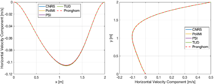
Figure 1:
The vertical velocity component distribution along AA` and BB` presented in Figure 2
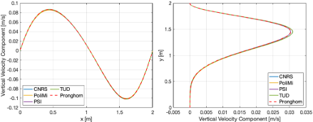
Figure 2:
The vertical velocity component distribution along BB` as the mesh is refined is presented in Figure 3.
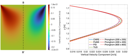
Figure 3:
Step 0.2:
This exercise models a steady state neutronic solution using Griffin. The problem geometry remains the same as step 0.1. The mesh is defined in a similar fashion to the earlier presentation and it is presented in this subsection for completeness.
[Mesh]
  type = MeshGeneratorMesh
  block_id = '1'
  block_name = 'cavity'
  [cartesian_mesh]
    type = CartesianMeshGenerator
    dim = 2
    dx = '1.0 1.0'
    ix = '100 100'
    dy = '1.0 1.0'
    iy = '100 100'
    subdomain_id = ' 1 1
                     1 1'
  []
  [assign_material_id]
    type = SubdomainExtraElementIDGenerator
    input = cartesian_mesh
    extra_element_id_names = 'material_id'
    subdomains = '1'
    extra_element_ids = '1'
  []
[]
(msr/cnrs/s02/cnrs_s02_griffin_neutronics.i)The input uses the fuel temperature to adjust the fuel density according to the expression
Although this adjustment of density is not useful in this step, it will be useful in the next step of the benchmark where the obtained temperature distribution is used to adjust the fuel salt density.
An eigenvalue solution of the multigroup neutron diffusion equation is performed with six energy groups. These characteristics and others including problem boundary conditions are defined in the TransportSystems
[TransportSystems]
  particle = neutron
  equation_type = eigenvalue
  G = 6
  VacuumBoundary = 'left bottom right top'
  [diff]
    scheme = CFEM-Diffusion
    n_delay_groups = 8
    family = LAGRANGE
    order = FIRST
    assemble_scattering_jacobian = true
    assemble_fission_jacobian = true
  []
[]
(msr/cnrs/s02/cnrs_s02_griffin_neutronics.i)Finally, the Executioner
[Executioner]
  type = Eigenvalue
  solve_type = PJFNKMO
  petsc_options_iname = '-pc_type -pc_factor_shift_type -pc_factor_mat_solver_package'
  petsc_options_value = 'lu NONZERO superlu_dist'
  free_power_iterations = 2
  line_search = none #l2
  l_max_its = 200
  l_tol = 1e-3
  nl_max_its = 200
  nl_rel_tol = 1e-6
  nl_abs_tol = 1e-8
[]
(msr/cnrs/s02/cnrs_s02_griffin_neutronics.i)Step 02 Results:
The results for this step include observing the fission rate density distribution and examining the influence of mesh refinement. Due to the length of the results, this documentation will only show the fission rate distribution along AA` which is presented in Figure 4.
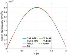
Figure 4:
For results on the mesh refinement, the reader is referred to the publication (Jaradat et al., 2024).
Step 0.3
In this exercise, the temperature field is obtained based on the velocity field and the power density profile. Thus, to solve this exercise, the solutions of steps 0.1 and 0.2 need to be obtained and provided in order to perform this step of the benchmark. Following is a description of the setup for this exercise input.
This requires a Navier-Stokes solve to obtain the velocity field and a neutronic solve to obtain the power density distribution. The main input in this step performs the linking between the neutronic solve and the Navier-Stokes solve. The main file defines a set of variables as follows
[AuxVariables]
  [U]
    order = CONSTANT
    family = MONOMIAL
    fv = true
    [AuxKernel]
      type = VectorMagnitudeAux
      x = vel_x
      y = vel_y
    []
  []
  [power_density]
    type = MooseVariableFVReal
  []
[]
(msr/cnrs/s03/cnrs_s03_ns_flow.i)These variables will be read from the solutions of step 0.1 and step 0.2. Auxiliary variables that are imported from the solutions of 0.1 and 0.2 are also defined as
[AuxVariables]
  [U]
    order = CONSTANT
    family = MONOMIAL
    fv = true
    [AuxKernel]
      type = VectorMagnitudeAux
      x = vel_x
      y = vel_y
    []
  []
  [power_density]
    type = MooseVariableFVReal
  []
[]
(msr/cnrs/s03/cnrs_s03_ns_flow.i)The boundary conditions are also defined in the Physics syntax as
        # Boundary conditions
        wall_boundaries = 'left right bottom top'
        momentum_wall_types = 'noslip noslip noslip noslip'
        momentum_wall_functors = '0 0; 0 0; 0 0; lid_function 0'
(msr/cnrs/s03/cnrs_s03_ns_flow.i)To obtain the solution of the previous two steps to be implemented in the solution of this step, a MultiApps
[MultiApps]
  [ns_flow]
    type = FullSolveMultiApp
    input_files = cnrs_s01_ns_flow.i
    cli_args = "Outputs/exodus=false;Outputs/active=''"
    execute_on = 'initial'
  []
  [griffin_neut]
    type = FullSolveMultiApp
    input_files = cnrs_s02_griffin_neutronics.i
    cli_args = "PowerDensity/family=MONOMIAL;PowerDensity/order=CONSTANT"
    execute_on = 'timestep_end'
  []
[]
(msr/cnrs/s03/cnrs_s03_ns_flow.i)where cnrs_s01_ns_flow.icnrs_s02_griffin_neutronics.iTransfers
[Transfers]
  # Initialization
  [x_vel]
    type = MultiAppCopyTransfer
    from_multi_app = ns_flow
    source_variable = 'vel_x'
    variable = 'vel_x'
    execute_on = 'initial'
  []
  [y_vel]
    type = MultiAppCopyTransfer
    from_multi_app = ns_flow
    source_variable = 'vel_y'
    variable = 'vel_y'
    execute_on = 'initial'
  []
  [pres]
    type = MultiAppCopyTransfer
    from_multi_app = ns_flow
    source_variable = 'pressure'
    variable = 'pressure'
    execute_on = 'initial'
  []

  # Multiphysics coupling
  [power_dens]
    type = MultiAppCopyTransfer
    from_multi_app = griffin_neut
    source_variable = 'power_density'
    variable = 'power_density'
    execute_on = 'timestep_end'
  []
  [temp]
    type = MultiAppCopyTransfer
    to_multi_app = griffin_neut
    source_variable = 'T_fluid'
    variable = 'tfuel'
    execute_on = 'timestep_end'
  []
[]
(msr/cnrs/s03/cnrs_s03_ns_flow.i)notice that the Navier-Stokes solve is expected to provide the velocity field. The neutronic solve is expected to provide the power density distribution. Note that the fuel temperature is used to adjust the density but it is not used to update the cross section.
Finally, characteristics of executing the problem are defined in the Executioner
[Executioner]
  # Solving the steady-state versions of these equations
  type = Steady
  solve_type = 'NEWTON'
  petsc_options_iname = '-pc_type -pc_factor_shift_type -pc_factor_mat_solver_package'
  petsc_options_value = 'lu NONZERO superlu_dist'
  nl_rel_tol = 1e-12
  nl_abs_tol = 1.5e-8
  nl_forced_its = 2
  automatic_scaling = true

  # MultiApps fixed point iteration parameters
  fixed_point_min_its = 2
  fixed_point_max_its = 50
  fixed_point_rel_tol = 1e-5
  fixed_point_abs_tol = 1e-5
[]
(msr/cnrs/s03/cnrs_s03_ns_flow.i)Step 03 Results
The fuel salt temperature distribution along AA` and BB` are in Figure 5
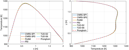
Figure 5:
References
- Mustafa K Jaradat, Namjae Choi, and Abdalla Abou-Jaoude.
Verification of griffin-pronghorn-coupled multiphysics code system against cnrs molten salt reactor benchmark.
Nuclear Science and Engineering, pages 1–34, 2024.[BibTeX]
@article{jaradat2024verification,
    author = "Jaradat, Mustafa K and Choi, Namjae and Abou-Jaoude, Abdalla",
    title = "Verification of Griffin-Pronghorn-Coupled Multiphysics Code System Against CNRS Molten Salt Reactor Benchmark",
    journal = "Nuclear Science and Engineering",
    pages = "1--34",
    year = "2024",
    publisher = "Taylor \\& Francis"
}
(msr/cnrs/s01/cnrs_s01_ns_flow.i)
# ==============================================================================
# Model description
# ------------------------------------------------------------------------------
# CNRS Benchmark model Created & modifed by Dr. Mustafa Jaradat and Dr. Namjae Choi
# November 22, 2022
# Step 0.1: Velocity field
# ==============================================================================
#   Tiberga, et al., 2020. Results from a multi-physics numerical benchmark for codes
#   dedicated to molten salt fast reactors. Ann. Nucl. Energy 142(2020)107428.
#   URL:http://www.sciencedirect.com/science/article/pii/S0306454920301262
# ==============================================================================

alpha = 2.0e-4
rho = 2.0e+3
cp = 3.075e+3
k = 1.0e-3
mu = 5.0e+1

[Mesh]
  type = MeshGeneratorMesh
  block_id = '1'
  block_name = 'cavity'
  [cartesian_mesh]
    type = CartesianMeshGenerator
    dim = 2
    dx = '1.0 1.0'
    ix = '100 100'
    dy = '1.0 1.0'
    iy = '100 100'
    subdomain_id = ' 1 1
                     1 1'
  []
[]

[Physics]
  [NavierStokes]
    [Flow]
      [flow]
        compressibility = 'incompressible'

        density = ${rho}
        dynamic_viscosity = 'mu'

        # Boussinesq parameters
        boussinesq_approximation = true
        gravity = '0 -9.81 0'
        thermal_expansion = ${alpha}
        ref_temperature = 900

        # Initial conditions
        initial_velocity = '0.5 0 0'
        initial_pressure = 1e5

        # Boundary conditions
        inlet_boundaries = 'top'
        momentum_inlet_types = 'fixed-velocity'
        momentum_inlet_functors = '0.5 0'

        wall_boundaries = 'left right bottom'
        momentum_wall_types = 'noslip noslip noslip'

        pin_pressure = true
        pinned_pressure_type = average
        pinned_pressure_value = 1e5

        # Numerical Scheme
        momentum_advection_interpolation = 'upwind'
        mass_advection_interpolation = 'upwind'
      []
    []
    [FluidHeatTransfer]
      [energy]
        initial_temperature = 900
        thermal_conductivity = 'k'
        specific_heat = 'cp'

        # Boundary conditions
        energy_inlet_types = 'fixed-temperature'
        energy_inlet_functors = 900
        energy_wall_types = 'heatflux heatflux heatflux'
        energy_wall_functors = '0 0 0'

        # Numerical Scheme
        energy_advection_interpolation = 'upwind'
        energy_two_term_bc_expansion = true
        energy_scaling = 1e-3
      []
    []
  []
[]

[FunctorMaterials]
  [functor_constants]
    type = ADGenericFunctorMaterial
    prop_names = 'k rho mu'
    prop_values = '${k} ${rho} ${mu}'
  []
  [cp]
    type = ADGenericFunctorMaterial
    # prop_names = 'cp dcp_dt'
    # prop_values = '${cp} 0'
    prop_names = 'cp'
    prop_values = '${cp}'
  []
[]

[Postprocessors]
  [Tfuel_avg]
    type = ElementAverageValue
    variable = T_fluid
  []
[]

[VectorPostprocessors]
  [AA_line_values_left]
    type = LineValueSampler
    start_point = '0 0.995 0'
    end_point = '2 0.995 0'
    variable = 'vel_x vel_y'
    num_points = 201
    execute_on = 'FINAL'
    sort_by = x
  []
  [AA_line_values_right]
    type = LineValueSampler
    start_point = '0 1.005 0'
    end_point = '2 1.005 0'
    variable = 'vel_x vel_y'
    num_points = 201
    execute_on = 'FINAL'
    sort_by = x
  []
  [BB_line_values_left]
    type = LineValueSampler
    start_point = '0.995 0 0'
    end_point = '0.995 2 0'
    variable = 'vel_x vel_y'
    num_points = 201
    execute_on = 'FINAL'
    sort_by = y
  []
  [BB_line_values_right]
    type = LineValueSampler
    start_point = '1.005 0 0'
    end_point = '1.005 2 0'
    variable = 'vel_x vel_y'
    num_points = 201
    execute_on = 'FINAL'
    sort_by = y
  []
[]

[Executioner]
  type = Transient
  start_time = 0.0
  end_time = 10000
  [TimeStepper]
    type = IterationAdaptiveDT
    dt = 0.1 # chosen to obtain convergence with first coupled iteration
    growth_factor = 2
  []
  steady_state_detection = true
  steady_state_tolerance = 1e-8
  steady_state_start_time = 10
  solve_type = 'NEWTON'
  petsc_options_iname = '-pc_type -pc_factor_shift_type -pc_factor_mat_solver_package'
  petsc_options_value = 'lu NONZERO superlu_dist'
  line_search = 'none'
  nl_rel_tol = 1e-7
  nl_abs_tol = 2e-7
  nl_max_its = 200
  l_max_its = 200
  automatic_scaling = true
[]

[Outputs]
  exodus = true
  [csv]
    type = CSV
    execute_on = 'FINAL'
  []
[]
(msr/cnrs/s02/cnrs_s02_griffin_neutronics.i)
# ==============================================================================
# Model description
# ------------------------------------------------------------------------------
# CNRS Benchmark model Created & modifed by Dr. Mustafa Jaradat and Dr. Namjae Choi
# November 22, 2022
# Step 0.2: Neutronics
# ==============================================================================
#   Tiberga, et al., 2020. Results from a multi-physics numerical benchmark for codes
#   dedicated to molten salt fast reactors. Ann. Nucl. Energy 142(2020)107428.
#   URL:http://www.sciencedirect.com/science/article/pii/S0306454920301262
# ==============================================================================

[GlobalParams]
  isotopes = 'pseudo'
  densities = 'densityf'
  library_file = '../xs/msr_cavity_xslib.xml'
  library_name = 'CNRS-Benchmark'
  grid_names = 'Tfuel'
  grid_variables = 'tfuel'
  is_meter = true
  plus = 1
[]

[Mesh]
  type = MeshGeneratorMesh
  block_id = '1'
  block_name = 'cavity'
  [cartesian_mesh]
    type = CartesianMeshGenerator
    dim = 2
    dx = '1.0 1.0'
    ix = '100 100'
    dy = '1.0 1.0'
    iy = '100 100'
    subdomain_id = ' 1 1
                     1 1'
  []
  [assign_material_id]
    type = SubdomainExtraElementIDGenerator
    input = cartesian_mesh
    extra_element_id_names = 'material_id'
    subdomains = '1'
    extra_element_ids = '1'
  []
[]

[TransportSystems]
  particle = neutron
  equation_type = eigenvalue
  G = 6
  VacuumBoundary = 'left bottom right top'
  [diff]
    scheme = CFEM-Diffusion
    n_delay_groups = 8
    family = LAGRANGE
    order = FIRST
    assemble_scattering_jacobian = true
    assemble_fission_jacobian = true
  []
[]

[PowerDensity]
  power = 1.0e9
  power_density_variable = power_density
  integrated_power_postprocessor = total_power
  power_scaling_postprocessor = Normalization
  family = LAGRANGE
  order = FIRST
[]

[AuxVariables]
  [tfuel]
    order = CONSTANT
    family = MONOMIAL
    initial_condition = 900
  []
  [densityf]
    order = CONSTANT
    family = MONOMIAL
    initial_condition = 1.0
  []
  [FRD]
    order  = FIRST
    family = L2_LAGRANGE
  []
[]

[AuxKernels]
  [density_fuel]
    type = ParsedAux
    block = 'cavity'
    variable = densityf
    coupled_variables = 'tfuel'
    expression = '(1.0-0.0002*(tfuel-900.0))'
    execute_on = 'INITIAL timestep_end'
  []
  [fission_rate_density]
    type = VectorReactionRate
    scalar_flux = 'sflux_g0 sflux_g1 sflux_g2 sflux_g3 sflux_g4 sflux_g5'
    cross_section = sigma_fission
    variable = FRD
    scale_factor = Normalization
    block = 'cavity'
  []
[]

[Materials]
  [fuel_salt]
    type = CoupledFeedbackMatIDNeutronicsMaterial
    block = 'cavity'
  []
[]

[Preconditioning]
  [SMP]
    type = SMP
    full = true
  []
[]
[Executioner]
  type = Eigenvalue
  solve_type = PJFNKMO
  petsc_options_iname = '-pc_type -pc_factor_shift_type -pc_factor_mat_solver_package'
  petsc_options_value = 'lu NONZERO superlu_dist'
  free_power_iterations = 2
  line_search = none #l2
  l_max_its = 200
  l_tol = 1e-3
  nl_max_its = 200
  nl_rel_tol = 1e-6
  nl_abs_tol = 1e-8
[]

[VectorPostprocessors]
  [AA_line_values_left]
    type = LineValueSampler
    start_point = '0 0.995 0'
    end_point = '2 0.995 0'
    variable = 'FRD'
    num_points = 201
    execute_on = 'FINAL'
    sort_by = x
  []
  [AA_line_values_right]
    type = LineValueSampler
    start_point = '0 1.005 0'
    end_point = '2 1.005 0'
    variable = 'FRD'
    num_points = 201
    execute_on = 'FINAL'
    sort_by = x
  []
  [BB_line_values_left]
    type = LineValueSampler
    start_point = '0.995 0 0'
    end_point = '0.995 2 0'
    variable = 'FRD'
    num_points = 201
    execute_on = 'FINAL'
    sort_by = y
  []
  [BB_line_values_right]
    type = LineValueSampler
    start_point = '1.005 0 0'
    end_point = '1.005 2 0'
    variable = 'FRD'
    num_points = 201
    execute_on = 'FINAL'
    sort_by = y
  []
[]

[Outputs]
  exodus = true
  [csv]
    type = CSV
    execute_on = 'FINAL'
  []
[]
(msr/cnrs/s03/cnrs_s03_ns_flow.i)
# ==============================================================================
# Model description
# ------------------------------------------------------------------------------
# CNRS Benchmark model Created & modifed by Dr. Mustafa Jaradat and Dr. Namjae Choi
# November 22, 2022
# Step 0.3: Temperature field
# ==============================================================================
#   Tiberga, et al., 2020. Results from a multi-physics numerical benchmark for codes
#   dedicated to molten salt fast reactors. Ann. Nucl. Energy 142(2020)107428.
#   URL:http://www.sciencedirect.com/science/article/pii/S0306454920301262
# ==============================================================================

rho   = 2.0e+3
cp    = 3.075e+3
k     = 1.0e-3
mu    = 5.0e+1
geometric_tolerance = 1e-3
cavity_l = 2.0
lid_velocity = 0.5

[UserObjects]
  [rc]
    type = INSFVRhieChowInterpolator
    u = vel_x
    v = vel_y
    pressure = pressure
  []
[]

[Mesh]
  type = MeshGeneratorMesh
  block_id = '1'
  block_name = 'cavity'
  [cartesian_mesh]
    type = CartesianMeshGenerator
    dim = 2
    dx = '1.0 1.0'
    ix = '100 100'
    dy = '1.0 1.0'
    iy = '100 100'
    subdomain_id = ' 1 1
                     1 1'
  []
[]

[Physics]
  [NavierStokes]
    [Flow]
      [flow]
        compressibility = 'incompressible'

        density = ${rho}
        dynamic_viscosity = 'mu'

        # Boussinesq parameters
        boussinesq_approximation = false
        gravity = '0 -9.81 0'

        # Initial conditions
        initial_velocity = '0.5 0 0'
        initial_pressure = 1e5

        # Boundary conditions
        wall_boundaries = 'left right bottom top'
        momentum_wall_types = 'noslip noslip noslip noslip'
        momentum_wall_functors = '0 0; 0 0; 0 0; lid_function 0'

        pin_pressure = true
        pinned_pressure_type = average
        pinned_pressure_value = 1e5

        # Numerical Scheme
        momentum_advection_interpolation = 'upwind'
        mass_advection_interpolation = 'upwind'
      []
    []
    [FluidHeatTransfer]
      [energy]
        initial_temperature = 900
        thermal_conductivity = 'k'
        specific_heat = 'cp'

        # Boundary conditions
        energy_wall_types = 'heatflux heatflux fixed-temperature fixed-temperature'
        energy_wall_functors = '0 0 0 1'

        # Volumetric heat sources and sinks
        ambient_temperature = 900
        ambient_convection_alpha = 1e6
        external_heat_source = power_density

        # Numerical Scheme
        energy_advection_interpolation = 'upwind'
        energy_two_term_bc_expansion = true
        energy_scaling = 1e-3
      []
    []
  []
[]

[FunctorMaterials]
  [functor_constants]
    type = ADGenericFunctorMaterial
    prop_names = 'cp k mu rho'
    prop_values = '${cp} ${k} ${mu} ${rho}'
  []
[]

[AuxVariables]
  [U]
    order = CONSTANT
    family = MONOMIAL
    fv = true
    [AuxKernel]
      type = VectorMagnitudeAux
      x = vel_x
      y = vel_y
    []
  []
  [power_density]
    type = MooseVariableFVReal
  []
[]

[Functions]
  [lid_function]
    type = ParsedFunction
    expression = 'if (x > ${geometric_tolerance}, if (x < ${fparse cavity_l - geometric_tolerance}, ${lid_velocity}, 0.0), 0.0)'
  []
[]

[Executioner]
  # Solving the steady-state versions of these equations
  type = Steady
  solve_type = 'NEWTON'
  petsc_options_iname = '-pc_type -pc_factor_shift_type -pc_factor_mat_solver_package'
  petsc_options_value = 'lu NONZERO superlu_dist'
  nl_rel_tol = 1e-12
  nl_abs_tol = 1.5e-8
  nl_forced_its = 2
  automatic_scaling = true

  # MultiApps fixed point iteration parameters
  fixed_point_min_its = 2
  fixed_point_max_its = 50
  fixed_point_rel_tol = 1e-5
  fixed_point_abs_tol = 1e-5
[]

[VectorPostprocessors]
  [AA_line_values_left]
    type = LineValueSampler
    start_point = '0 0.995 0'
    end_point = '2 0.995 0'
    variable = 'T_fluid'
    num_points = 201
    execute_on = 'FINAL'
    sort_by = x
  []
  [AA_line_values_right]
    type = LineValueSampler
    start_point = '0 1.005 0'
    end_point = '2 1.005 0'
    variable = 'T_fluid'
    num_points = 201
    execute_on = 'FINAL'
    sort_by = x
  []
  [BB_line_values_left]
    type = LineValueSampler
    start_point = '0.995 0 0'
    end_point = '0.995 2 0'
    variable = 'T_fluid'
    num_points = 201
    execute_on = 'FINAL'
    sort_by = y
  []
  [BB_line_values_right]
    type = LineValueSampler
    start_point = '1.005 0 0'
    end_point = '1.005 2 0'
    variable = 'T_fluid'
    num_points = 201
    execute_on = 'FINAL'
    sort_by = y
  []
[]

[MultiApps]
  [ns_flow]
    type = FullSolveMultiApp
    input_files = cnrs_s01_ns_flow.i
    cli_args = "Outputs/exodus=false;Outputs/active=''"
    execute_on = 'initial'
  []
  [griffin_neut]
    type = FullSolveMultiApp
    input_files = cnrs_s02_griffin_neutronics.i
    cli_args = "PowerDensity/family=MONOMIAL;PowerDensity/order=CONSTANT"
    execute_on = 'timestep_end'
  []
[]

[Transfers]
  # Initialization
  [x_vel]
    type = MultiAppCopyTransfer
    from_multi_app = ns_flow
    source_variable = 'vel_x'
    variable = 'vel_x'
    execute_on = 'initial'
  []
  [y_vel]
    type = MultiAppCopyTransfer
    from_multi_app = ns_flow
    source_variable = 'vel_y'
    variable = 'vel_y'
    execute_on = 'initial'
  []
  [pres]
    type = MultiAppCopyTransfer
    from_multi_app = ns_flow
    source_variable = 'pressure'
    variable = 'pressure'
    execute_on = 'initial'
  []

  # Multiphysics coupling
  [power_dens]
    type = MultiAppCopyTransfer
    from_multi_app = griffin_neut
    source_variable = 'power_density'
    variable = 'power_density'
    execute_on = 'timestep_end'
  []
  [temp]
    type = MultiAppCopyTransfer
    to_multi_app = griffin_neut
    source_variable = 'T_fluid'
    variable = 'tfuel'
    execute_on = 'timestep_end'
  []
[]

[Outputs]
  exodus = true
  [csv]
    type = CSV
    execute_on = 'FINAL'
  []
[]