Subchannel Model for the Toshiba 37-Pin Benchmark
Contact: Mauricio Tano, mauricio.tanoretamales.at.inl.gov
Model link: Toshiba 37-Pin Subchannel Model
Benchmark Description
The Toshiba 37-pin benchmark is based on liquid sodium experiments conducted by the Toshiba Corporation Nuclear Engineering Laboratory in Japan (Namekawa et al., 1984). Its assembly consists of four outer rings of electrically heated rods. However, the resistances in the electrically heated rods are adapted to reproduce a chopped cosine power distribution in the axial direction. All heating rods are assumed to have the same power distribution. The cross section of the fuel assembly is presented in Figure 1. In this figure the numbering of the rods and the subchannels are described. The analyzed quantity of interest is the temperature distribution at the outlet of the assembly. Due to symmetry, it is enough to analyze the temperature distributions over a symmetry line. In this case, following experiment reported results, we take a south-to-north line in the fuel assembly. This one involves, in south to north ordering, subchannels 72, 49, 32, 20, 10, 4, 3, 2, 1, 7, 14, 26, 39, and 58.
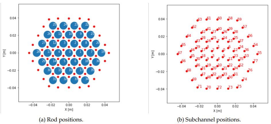
Figure 1: Rod and subchannel positions and numbering adopted for the Toshiba 37-pin benchmark. (a) Position and numbering of the heated rods with the subchannel center indicated with red dots. (b) Center position and numbering of the suchannels.
The characteristics of Toshiba's benchmark are provided in Table 1.
Table 1: Design and operational parameters for Toshiba's 37-pin benchmark.
| Experiment Parameter (unit) | Value |
|---|---|
| Number of pins (-) | 37 |
| Rod Pitch (cm) | 0.787 |
| Rod Diameter (cm) | 0.650 |
| Wire wrap diameter (cm) | 0.132 |
| Wire wrap axial pitch (cm) | 30.70 |
| Flat-to-flat duct distance (cm) | 5.04 |
| Inlet length (cm) | - |
| Heated length (cm) | 93.00 |
| Outlet length (cm) | - |
| Outlet pressure (Pa) | 1.01E5 |
| Inlet Temperature (K) | Experiment dependent |
| Power profile (-) | Chopped cosine (peaking factor 1.21) |
Three flow configurations with reducing axial mass flow rate are selected for the validation exercise. These configurations are presented in Table 2.
Table 2: Validation cases selected in the Toshiba benchmark
| Naming | Run ID | Rod Power (W/cm) | Inlet temperature () | Flow rate (m/s) | Reynolds number |
|---|---|---|---|---|---|
| High flow rate | B37P02 | 15.57 | 484.3 | 1.48E-03 | 1.12E4 |
| Medium flow rate | 0C37P06 | 11.92 | 476.5 | 3.34E-04 | 2.81E3 |
| Low flow rate | E37P13 | 3.89 | 479.4 | 1.07E-04 | 7.39E2 |
Subchannel Input
General Parameters
The general parameters on the experimental conditions are described here below. They set up the boundary conditions for the high-flow-rate test case.
 T_in = 660
# [1e+6 kg/m^2-hour] turns into kg/m^2-sec
mass_flux_in = ${fparse 1e+6 * 37.00 / 36000.*0.5}
P_out = 2.0e5 # Pa
Mesh
The meshing in subchannel uses a custom TriSubChannelMeshGenerator. This generates a mesh of 1D channel segments connected in 3D. The subchannel positions are automatically generated by specifying the number of radial rings, the flat to flat distance of the duct, and the rod pitch. The number of axial cells in which the domain is discretized is specified by n_cells. For more information about the mesh generator, please consult the website documentation on subchannel.
[TriSubChannelMesh]
  [subchannel]
    type = SCMTriSubChannelMeshGenerator
    nrings = 4
    n_cells = 100
    flat_to_flat = 0.085
    heated_length = 1.0
    pin_diameter = 0.01
    pitch = 0.012
    dwire = 0.002
    hwire = 0.0833
    spacer_z = '0 0.2 0.4 0.6 0.8'
    spacer_k = '0.1 0.1 0.1 0.1 0.10'
  []
[]
Fluid Properties
The fluid properties block specifies the thermophysical properties used in the subchannel solve. Sodium properties are used in this case.
[FluidProperties]
  [sodium]
    type = PBSodiumFluidProperties
  []
[]
SubChannel
The SubChannel block specifies the solver to be used in the subchannel solve. The type of problem used in this case is a liquid metal subchannel problem that uses sodium fluid properties. The parameters beta and C_T are used to model the crossflow and cross enthalpy-fluxes. Different solve procedures can be applied. In this case, we use an implicit, monolithic solve.
[SubChannel]
  type = TriSubChannel1PhaseProblem
  fp = sodium
  n_blocks = 1
  P_out = 2.0e5
  CT = 1.0
  compute_density = true
  compute_viscosity = true
  compute_power = true
  P_tol = 1.0e-6
  T_tol = 1.0e-3
  implicit = true
  segregated = false
  staggered_pressure = false
  verbose_multiapps = true
  verbose_subchannel = false
[]
Initial Conditions
This block specifies the initial conditions for the AuxVariables utilized in the subchannel solve. The linear heat flux initialization requires an external file that defines the relative power per fuel pin. In this case, this file is named "pin_power_profile_37.txt"
[ICs]
  [S_IC]
    type = SCMTriFlowAreaIC
    variable = S
  []

  [w_perim_IC]
    type = SCMTriWettedPerimIC
    variable = w_perim
  []

  [q_prime_IC]
    type = SCMTriPowerIC
    variable = q_prime
    power = 1.000e5 # W
    filename = "pin_power_profile_37.txt"
  []

  [T_ic]
    type = ConstantIC
    variable = T
    value = ${T_in}
  []

  [P_ic]
    type = ConstantIC
    variable = P
    value = ${P_out}
  []

  [DP_ic]
    type = ConstantIC
    variable = DP
    value = 0.0
  []
  [Viscosity_ic]
    type = ViscosityIC
    variable = mu
    p = ${P_out}
    T = T
    fp = sodium
  []

  [rho_ic]
    type = RhoFromPressureTemperatureIC
    variable = rho
    p = P
    T = T
    fp = sodium
  []

  [h_ic]
    type = SpecificEnthalpyFromPressureTemperatureIC
    variable = h
    p = P
    T = T
    fp = sodium
  []

  [mdot_ic]
    type = ConstantIC
    variable = mdot
    value = 0.0
  []
[]
Auxiliary Kernels
Auxiliary kernels are used to apply the boundary conditions on pressure, temperature, and mass flow rate.
[AuxKernels]
  [P_out_bc]
    type = ConstantAux
    variable = P
    boundary = outlet
    value = ${P_out}
    execute_on = 'timestep_begin'
  []
  [T_in_bc]
    type = ConstantAux
    variable = T
    boundary = inlet
    value = ${T_in}
    execute_on = 'timestep_begin'
  []
  [mdot_in_bc]
    type = SCMMassFlowRateAux
    variable = mdot
    boundary = inlet
    area = S
    mass_flux = ${mass_flux_in}
    execute_on = 'timestep_begin'
  []
[]
Executioner
The executioner can be Steady or Transient. The tolerances which are set in the [Executioner] block are not used in the subchannel problem.
[Executioner]
  type = Steady
[]
MultiApp system
A MultiApp is used for transferring the subchannel solution into a detailed mesh for visualization.
[MultiApps]
  [viz]
    type = FullSolveMultiApp
    input_files = "toshiba_37_pin_viz.i"
    execute_on = "timestep_end"
  []
[]
A custom transfer, MultiAppDetailedSolutionTransfer, is used for this purpose.
[Transfers]
  [xfer]
    type = SCMSolutionTransfer
    to_multi_app = viz
    variable = 'mdot SumWij P DP h T rho mu q_prime S displacement w_perim'
  []
[]
The detailed mesh uses a DetailedTriSubChannelMeshGenerator and the solution variables are populated by the transfer.
[MultiApps]
  [viz]
    type = FullSolveMultiApp
    input_files = "toshiba_37_pin_viz.i"
    execute_on = "timestep_end"
  []
[]
Results
An example flow distribution for the high flow-rate case is depicted in Figure 2. The figures have been scaled by 0.25 in the axial direction. As graphically observed, a flat temperature profile is obtained in the bulk of the fuel assembly. In this experiment, the ratio of gap-distance to pitch produces a significantly larger mass flow in the outer subchannels as observed in Figure 2a. This causes the outer subchannnels to be significantly colder than the center ones. Thus, the expected temperature distribution is flat in the central region of the assembly with sharp drops next to the wrapper. Finally, it can be observed in Figures 2a and 2b that due to the significant difference between flow rates at the outer and center subchannel, there is a considerable flow development length in the entry to the fuel assembly. Inlet velocity conditions were unclear in the experiment report (Namekawa et al., 1984) and, hence, uniform mass flow at the inlet was assumed. If the assumption of uniform inlet flow rates turns out to be incorrect, a small deterioration of accuracy of the predicted outlet temperature can be expected. However, we observe that the flow rates fully develop before the outlet of the assembly, which suggests that this initial condition will have little effect over the analyzed temperature distribution at the outlet of the fuel assembly.
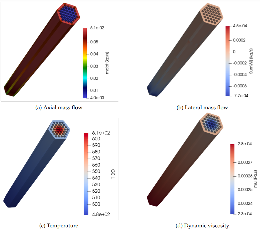
Figure 2: Example of simulation results for the high-flow test case in the Toshiba 37-pin benchmark. (a) Distribution of axial mass flow. (b) Distribution of lateral mass flow. (c) Distribution of temperature. (d) Distribution of dynamic viscosity due to heating.
The results obtained for the high-, medium-, and low- flow-rate validation cases are presented in Figure 3. We compare the results obtained with the present code with the ones obtained in the experiments and the SUBAC code (Sun et al., 2018). We have selected SUBAC for the code-to-code comparison since it is to our knowledge the subchannel code for wire-wrapped SFRs, with openly available results, that presented the best agreements between the code predictions and the experiment measurements for the current benchmark.
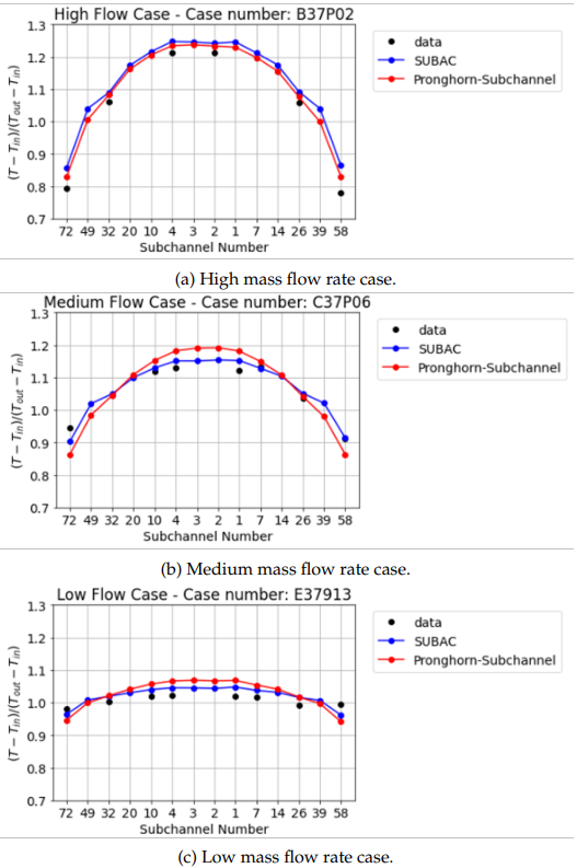
Figure 3: Comparison of results obtained for Toshiba 37-pin case between experimental measurements, the SUBAC code, and the current code. (a) High mass flow case. (b) Medium mass flow case. (c) Low mass flow case.
As observed in Figure 3, for the high mass flow rate case, the present model predicts results closer to the experimental results than SUBAC. This is expected, since the turbulent cross-flow calibration should still improve the prediction for the present case. However, when comparing the results predicted for the medium- and low-flow-rate cases in Figures 3b and 3c, respectively, we observe that our models over-predict the temperature distributions when compared to SUBAC. Further analysis determined that the more peaked distribution of temperatures predicted by SCM towards the center of the assembly may be produced by an over-prediction of the mixing rates, which yields larger than expected flows in the outer channels.
Sample output for this model, in the gold folder, is hosted on LFS. Please refer to LFS instructions to download it.
References
- F Namekawa, A Ito, and K Mawatari.
Buoyancy effects on wire-wrapped rod bundle heat transfer in an lmfbr fuel assembly.
In AIChE symposium series, volume 80, 128–133. 1984.[BibTeX]
- RL Sun, DL Zhang, Y Liang, MJ Wang, WX Tian, SZ Qiu, and GH Su.
Development of a subchannel analysis code for sfr wire-wrapped fuel assemblies.
Progress in Nuclear Energy, 104:327–341, 2018.[BibTeX]