Subchannel Model for the Oak Ridge National Laboratory (ORNL) 19-Pin Benchmark
Contact: Mauricio Tano, mauricio.tanoretamales.at.inl.gov
Model link: ORNL 19-Pin Subchannel Model
Benchmark description
The ORNL 19-pin experiment was built at Oak Ridge National Laboratory for studying the thermal-hydraulic flow characteristics in SFR assemblies as described in (Fontana et al., 1974). The cross section of the experimental facility is depicted in Figure 1. The validation exercise was done for test series 2 of this experiment. In this series, the fuel rods of the experiment were heated by 19 identical electric cartridges. The configuration and external heat fluxes of these cartidges match typical values expected for SFRs. The measurements in test series 2 focused on the distribution of temperatures at the exit of the fuel assembly, the duct walls, and the rod bundle. The nature of the heat source and the lack of neighboring assemblies make the distribution of temperatures at the rod bundle and duct atypical for LMRs. Therefore, this data was deemed of secondary importance for validating the subchannel code. In contrast, the distribution of temperatures at the exit of the fuel assembly is indicative of the heating of the coolant and flow mixing in the fuel bundle, which is expected to be representative of the one in an actual SFR. Therefore, we have focused our validation work in predicting the distribution of temperatures at the exit of the fuel assembly.
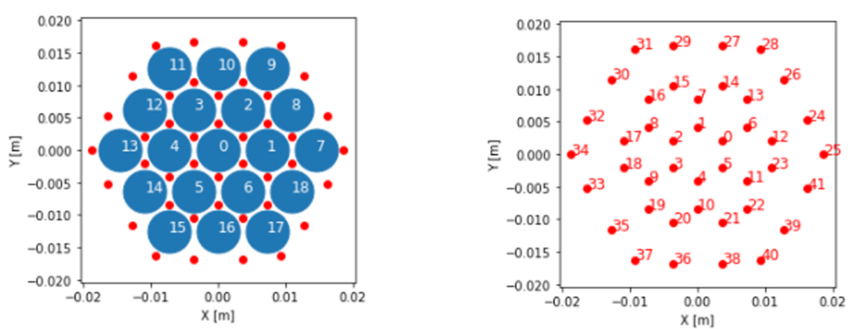
Figure 1: Left: heating rod positions for the experiment. Right: subchannel positions in the experiment.
The design parameters for test series 2 of the ORNL 19-pin experiment are presented in Table 1. Pressure is assumed to be constant at the outlet of the assembly and temperature and mass flux are assumed to be constant at its inlet. The fuel bundle is divided between inlet, heated, and outlet sections along the rod in increasing elevation. A nonzero linear heat rate is only assigned to the heated part of the rod, while no power is imposed at the inlet and outlet sections.
Table 1: Design and operational parameters for ORNL's 19-pin benchmark.
| Experiment Parameter (unit) | Value |
|---|---|
| Number of pins (-) | 19 |
| Rod Pitch (cm) | 0.726 |
| Rod Diameter (cm) | 0.584 |
| Wire wrap diameter (cm) | 0.142 |
| Wire wrap axial pitch (cm) | 30.48 |
| Flat-to-flat duct distance (cm) | 3.41 |
| Inlet length (cm) | 40.64 |
| Heated length (cm) | 53.34 |
| Outlet length (cm) | 7.62 |
| Outlet pressure (Pa) | 1.01E5 |
| Inlet Temperature (K) | 588.5 |
| Power profile (-) | Uniform |
Due to hexagonal symmetry in the experiment, the temperature distribution has been measured over the subchannels that approximately lie on a the diagonal line that connects the opposed vertices in the duct. The orientation of the meassuring line connects the south-west vertex to the north-east one. For our numbering convention, this lines includes subchannels 37, 36, 20, 10, 4, 1, 12, and 28.
Three different flow and heating configurations were evaluated for the experiment validation. These configurations are summarized in Table 2.
Table 2: Validation cases selected in the ORNL benchmark
| Naming | Run ID | Rod Power (W/cm) | Flow rate (m/s) | Reynolds number |
|---|---|---|---|---|
| High flow rate | 022472-hf | 318.2 | 3.47E-03 | 6.72E4 |
| Medium flow rate | 020372 | 30.8 | 3.15E-04 | 7.35E3 |
| Low flow rate | 022472-lf | 4.9 | 4.67E-05 | 9.05E2 |
Subchannel input
General parameters
The general parameters on the experimental conditions are described here below. They set up the boundary conditions for the high-flow-rate test case.
 T_in = 588.5
 flow_area = 0.0004980799633447909 #m2
 mass_flux_in = ${fparse 55*3.78541/10/60/flow_area}  # [1e+6 kg/m^2-hour] turns into kg/m^2-sec
 P_out = 2.0e5 # Pa
Mesh
The meshing in subchannel uses a custom TriSubChannelMeshGenerator. This one generates a mesh of 1D channel segments connected in 3D. The subchannel positions are automatically generated by specifying the number of radial rings, the flat to flat distance of the duct, and the rod pitch. The number of axial cells in which the domain is discretized is specified by n_cells. For more information about the mesh generator, please consult the subchannel documentation.
[TriSubChannelMesh]
  [subchannel]
    type = SCMTriSubChannelMeshGenerator
    nrings = 3
    n_cells = 40
    flat_to_flat = 3.41e-2
    heated_length = 0.5334
    unheated_length_entry = 0.4064
    unheated_length_exit = 0.0762
    pin_diameter = 5.84e-3
    pitch = 7.26e-3
    dwire = 1.42e-3
    hwire = 0.3048
    spacer_z = '0'
    spacer_k = '0'
  []
[]
Fluid Properties
The fluid properties block specifies the thermophysical properties used in the subchannel solve. Sodium properties are used in this case.
[FluidProperties]
  [sodium]
    type = PBSodiumFluidProperties
  []
[]
SubChannel
The SubChannel block specifies the solver to be used in the subchannel solve. The type of problem used in this case is a liquid metal subchannel problem that uses sodium fluid properties. The parameters beta and C_T are used to model the crossflow and cross enthalpy-fluxes. Different solve procedures can be applied. In this case, we use an explicit, segregated solve. For more information about the mesh generator, please consult the website documentation on subchannel.
[SubChannel]
  type = TriSubChannel1PhaseProblem
  fp = sodium
  n_blocks = 1
  P_out = 2.0e5
  CT = 2.6
  compute_density = true
  compute_viscosity = true
  compute_power = true
  implicit = true
  segregated = false
  P_tol = 1e-4
  T_tol = 1e-4
  staggered_pressure = false
  verbose_multiapps = true
  verbose_subchannel = true
  interpolation_scheme = upwind
[]
Initial Conditions
This block specifies the initial conditions for the AuxVariables utilized in the subchannel solve. The linear heat flux initialization requires an external file that defines the relative power per fuel pin. In this case, this file is named "pin_power_profile_19.txt"
[ICs]
  [S_IC]
    type = SCMTriFlowAreaIC
    variable = S
  []

  [w_perim_IC]
    type = SCMTriWettedPerimIC
    variable = w_perim
  []

  [q_prime_IC]
    type = SCMTriPowerIC
    variable = q_prime
    power = 322525.0 #W
    filename = "pin_power_profile_19.txt"
  []

  [T_ic]
    type = ConstantIC
    variable = T
    value = ${T_in}
  []

  [P_ic]
    type = ConstantIC
    variable = P
    value = 0.0
  []

  [DP_ic]
    type = ConstantIC
    variable = DP
    value = 0.0
  []

  [Viscosity_ic]
    type = ViscosityIC
    variable = mu
    p = ${P_out}
    T = T
    fp = sodium
  []

  [rho_ic]
    type = RhoFromPressureTemperatureIC
    variable = rho
    p = ${P_out}
    T = T
    fp = sodium
  []

  [h_ic]
    type = SpecificEnthalpyFromPressureTemperatureIC
    variable = h
    p = ${P_out}
    T = T
    fp = sodium
  []

  [mdot_ic]
    type = ConstantIC
    variable = mdot
    value = 0.0
  []
[]
Auxiliary Kernels
Auxiliary kernels are used to apply the boundary conditions on pressure, temperature, and mass flow rate.
[AuxKernels]
  [T_in_bc]
    type = ConstantAux
    variable = T
    boundary = inlet
    value = ${T_in}
    execute_on = 'timestep_begin'
  []
  [mdot_in_bc]
    type = SCMMassFlowRateAux
    variable = mdot
    boundary = inlet
    area = S
    mass_flux = ${mass_flux_in}
    execute_on = 'timestep_begin'
  []
[]
Boundary conditions are set in the subchannel problem through the boundary values of auxiliary variables. This is a more succinct alternative to using several postprocessors, one for each channel. There is also no explicit [BCs] block in subchannel inputs, as the boundary condition is handled by the custom TriSubChannel1PhaseProblem problem.
Executioner
The executioner can be Steady or Transient. The solver tolerances which can be set in this block are not used in the subchannel problem.
[Executioner]
  type = Steady
[]
MultiApp system
A MultiApp is used for transferring the subchannel solution into a detailed mesh for visualization.
[MultiApps]
  [viz]
    type = FullSolveMultiApp
    input_files = "ornl_19_pin_viz.i"
    execute_on = "timestep_end"
  []
[]
A custom transfer, MultiAppDetailedSolutionTransfer, is used for this purpose.
[Transfers]
  [xfer]
    type = SCMSolutionTransfer
    to_multi_app = viz
    variable = 'mdot SumWij P DP h T rho mu q_prime S'
  []
[]
The detailed mesh uses a DetailedTriSubChannelMeshGenerator and the solution variables are populated by the transfer.
################################################################################
## SFR ORNL 19 pin assembly benchmark                                         ##
## MultiApp for visualization of output                                       ##
## POC : Mauricio Tano, mauricio.tanoretamales at inl.gov                     ##
################################################################################
## If using or referring to this model, please cite as explained in
## https://mooseframework.inl.gov/virtual_test_bed/citing.html

[Mesh]
  [subchannel]
    type = SCMDetailedTriSubChannelMeshGenerator
    nrings = 3
    n_cells = 40
    flat_to_flat = 3.41e-2
    heated_length = 0.5334
    unheated_length_entry = 0.4064
    unheated_length_exit = 0.0762
    pin_diameter = 5.84e-3
    pitch = 7.26e-3
  []
[]

[AuxVariables]
  [mdot]
  []
  [SumWij]
  []
  [P]
  []
  [DP]
  []
  [h]
  []
  [T]
  []
  [rho]
  []
  [mu]
  []
  [S]
  []
  [w_perim]
  []
  [q_prime]
  []
[]

[Problem]
  type = NoSolveProblem
[]

[Outputs]
  exodus = true
[]

[Executioner]
  type = Steady
[]
Results
The key factor dominating the temperature profile in the outlet of the domain is the competing effect between heat convection and heat conduction in the coolant. An example of the axial and lateral mass flow rates and the temperature and viscosity fields obtained for a high-flow-rate configuration in the ORNL 19-pin benchmark is presented in Figure 2. The flow rapidly develops over the assembly. However, there is a significantly larger flow field in the outer gaps of the rod bundle. This results in the outer rod and channels being colder than the center ones. The temperature difference between outlet and inner subchannels increases with the increasing mass flow rate. There is a small competing effect due to the viscosity in the center of the channels being smaller due to heating, but this effect is of second order compared with the flow driven by the pressure drop effects. However, as mass flow decreases, heat conduction in the sodium coolant starts dominating over heat convection and, hence, the temperature profiles become flatter at the exit. In summary, the temperature distribution measured at the outlet of the assembly can be regulated by the balance between convection and conduction, which is experimentally regulated by changing the axial mass flux and the power at the rod bundles.
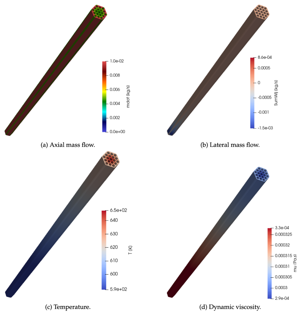
Figure 2: Example of simulation results for the high-flow test case in the ORNL-19 benchmark. (a) Distribution of axial mass flow. (b) Distribution of lateral mass flow. (c) Distribution of temperature. (d) Distribution of dynamic viscosity due to heating.
The results obtained are compared against the experimental values and the SUBAC and MATRA-LMR codes in Figure 3. It is observed that for every single case our code predicts temperature distribution values that match more closely the experimental results.
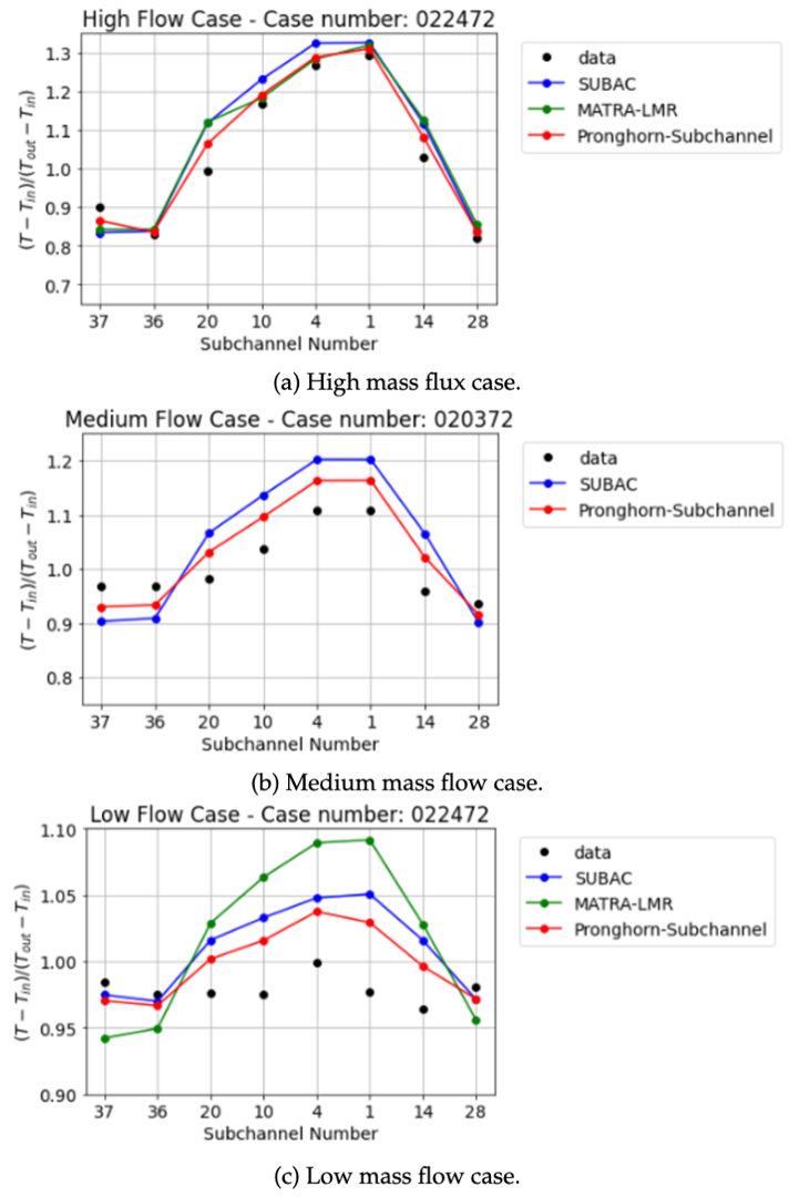
Figure 3: Comparison of results obtained for ORNL-19 pin case between experimental measurements, the SUBAC code, the MATRA-LMR code, and the current code. (a) High mass flow case. (b) Medium mass flow case. (c) Low mass flow case
Sample output for this model, in the gold folder, is hosted on LFS. Please refer to LFS instructions to download it.
References
- MH Fontana, RE MacPherson, PA Gnadt, LF Parsly, and JL Wantland.
Temperature distribution in the duct wall and at the exit of a 19-rod simulated lmfbr fuel assembly (ffm bundle 2a).
Nuclear Technology, 24(2):176–200, 1974.[BibTeX]