Symmetric Sector Bowing - Linear Thermal Gradient (IAEA VP3A)
Contact: Nick Wozniak, nwozniak.at.anl.gov
Model link: Hexagonal Duct Bowing Model
High Level Summary of Model
This model examines the restrained thermal bowed deformation of a 3D hexagonal assembly (duct) which is subject to thermal gradients along the axial and radial directions bowing into a sector of a reactor core. The ducts are mechanically fixed at the bottom. The model specification is based on Verification Problem 3A (VP3A) in the series of benchmark problems published in IAEA (1990) to support the verification and validation of Liquid Metal Fast Breeder Reactor (LMFBR) analysis codes organized by The International Atomic Energy Agency (IAEA)’s International Working Group on Fast Reactors (IWGFR). This model employs the MOOSE Tensor Mechanics Module to model the thermo-mechanical deformation response due to the thermal gradients in the duct, and the Contact Module to model the inter-assembly contact at specific locations along the ducts. This type of deformation is present in liquid-metal cooled fast reactors and serves as an important reactivity feedback effect. The results obtained from this MOOSE-based model demonstrate proper set up of a single assembly thermal duct bowing problem which can be used to build larger and more complex models.
Computational Model Description
In this example, known as IAEA Verification Problem 3A (VP3A), a known linearly varying thermal gradient is applied to the hexagonal duct, along the axial height in the active core region, as shown in Figure 1. Below the active core, the duct is at 400°C which varies linearly from the core inlet to 550°C at the left corner midwall and 500°C at the far right corner midwall. Along the cross-section, the temperature follows a linear gradient at each axial location. Above the active core, the temperatures are held constant from the core outlet to the top of the duct. The cross-sectional thermal gradient produces a differential thermal expansion where the hotter side of the duct expands more than the cooler side, causing a bowed displacement from hot side towards cold side. The duct is a single assembly of a reactor core sector, shown in Figure 2. The model for VP3A is a 60° sector of the hexagonal-assembly core freed from the rest of the core. In this configuration, the center duct thermally bows in the y-axis direction into the top 60° sector, which has a free boundary around the edges as shown in Figure 2. All the other ducts remain at 400°C.
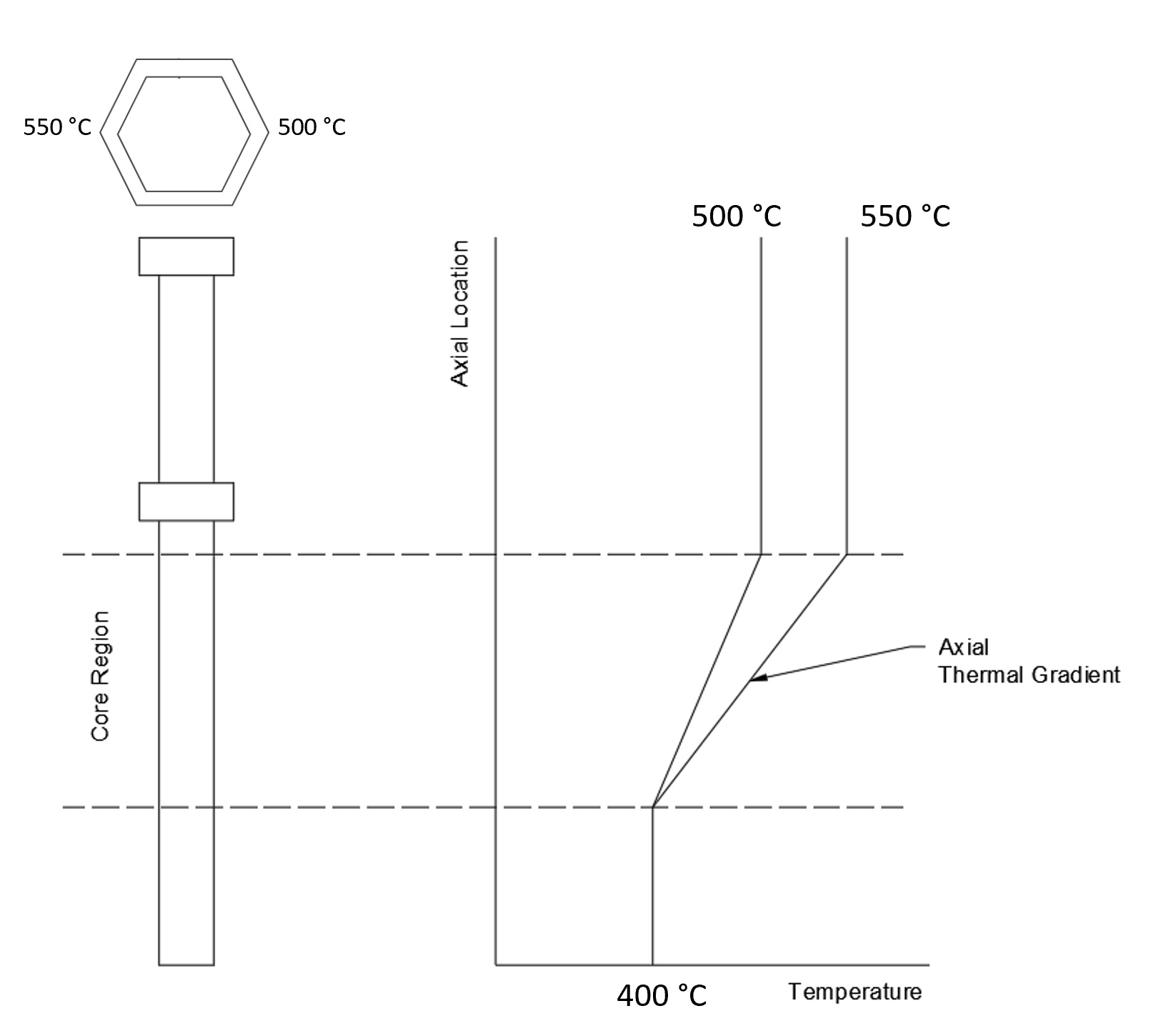
Figure 1: Representation of thermal gradient along duct axial location, from 400°C below the core extending to 500°C and 550°C on opposite corners of the duct.
 © IAEA).](../../media/hex_duct_bowing/vp3a_sector.png)
Figure 2: IAEA VP3A core layout showing the free boundary around the sector with red dashed lines and the bowing direction with a blue arrow, (right) sector removed from the full core (Adapted from IAEA (1990) © IAEA).
Figure 3 shows the geometry of the duct in both elevation and cross-section view, with the primary geometric parameters labeled. Table 1 summarizes the values for the geometric parameters. The duct is 4000 mm long, with the active core region extending from 1500 mm along the axial direction to 2500 mm. There is an above core load pad (ACLP) located at 3000 mm axial height. Normally in a Fast Reactor design there is also a top load pad (TLP) at the top of the duct, but in this design, a TLP is omitted even though contact is assumed to occur at the top of the duct. The duct is a sharp cornered hexagon with a distance between the mid-walls of the corners of 150 mm and a wall thickness of 3 mm at room temperature, 20°C. The ACLP has a thickness on top of the duct wall of 2.75 mm and an arbitrary height of 100 mm. The duct and load pad are made of a fictitious steel material with constant material properties (not dependent on temperature) which are given in Table 2.

Figure 3: Schematic showing duct model geometric parameters.
Table 1: Duct Geometric Parameters.
| Parameter | Value (mm) |
|---|---|
| Duct | |
| Corner-to-corner | 150 |
| Assembly Length | 4000 |
| Wall Thickness | 3 |
| ACLP Thickness | 2.75 |
| ACLP Height | 100 |
| Axial Location | |
| Core Bottom | 1500 |
| Core Top | 2500 |
| Above Core Load Pad (ACLP) | 3000 |
Table 2: Duct Material Properties.
| Property | Value |
|---|---|
| Young's Modulus | |
| Poisson's Ratio | |
| Coefficient of Thermal Expansion |
The geometry and phenomenon in this model are relevant to core-bowing phenomena present in liquid-metal cooled fast reactor design and analysis. The core bowing present in reactor assemblies induces reactivity feedback effects due to sensitivity of fast neutron reactors to leakage pathways. The MOOSE Reactor Module is used to generate the duct mesh, and the MOOSE Tensor Mechanics module is used to calculate the thermo-mechanical response of the duct due to differential thermal expansion and the MOOSE Contact Module is used to simulate the contact behavior between ducts as they bow into one another. This work was originally performed as part of an assessment of the MOOSE Tensor Mechanics module for calculating radial core expansion for fast reactors in Wozniak et al. (2021) and Wozniak and Shemon (2022) funded under the NEAMS program. The temperature along the cold () corner of the duct is defined by Eq. (1):
(1)
The temperature along the hot () corner of the duct is defined by Eq. (2):
(2)
Due to the complex contact interaction between multiple assemblies at different axial locations, there is no closed-form solution for this example. The problem must be solved numerically with iteration steps to ensure contact enforcement. Due to the nonlinear behavior of the contact interaction, the model was defined as a transient simulation with the temperature applied incrementally over the pseudo-time steps from 0 to 1s incremented by 0.1s.
Mesh Block
The core sector was meshed using CUBIT v15.5 SNL (2019). The mesh is defined with the file parameter referencing the mesh file in the local directory. Since the dimensions were provided at room temperature, the model was created with dimensions at 400°C to consider the initial warm up phase from 20°C and grid plate expansion, which increases the pitch and gaps. To reduce computational expense, a symmetric model was set up with symmetry along the YZ plane. In addition, only ducts 1, 3, 10, and 11 were modeled because the IAEA report results show contact only between ducts 1 and 3 at the TLP and between ducts 3 and 10 at the ACLP. For computational efficiency, the ducts beyond 10 and 11 were not included since they are at constant 400 °C, and ducts 10 and 11 should not deflect far enough to close the gap between the outside ducts. The mesh is shown in Figure 4 with a top-down view showing the duct numbering consistent with Figure 2 to show which ducts are included, and an isometric view.
[Mesh]
  file = iaea_vp3a_symmetric_mesh.e
  patch_update_strategy = auto
  patch_size = 20
  partitioner = centroid
  centroid_partitioner_direction = z

  allow_renumbering = false
[]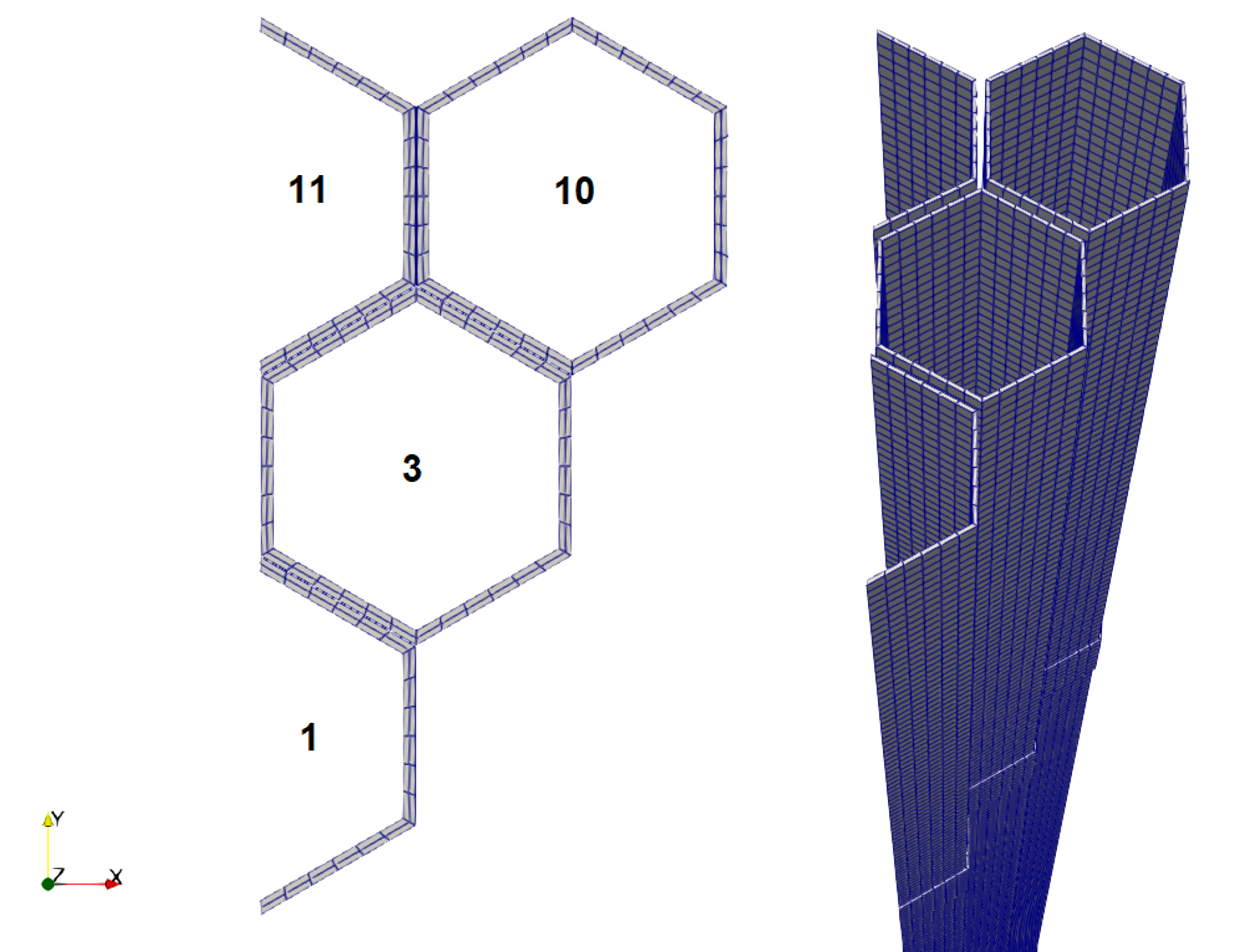
Figure 4: VP3A symmetric model mesh, with the (left) top-down view at the ACLP elevation and (right) isometric view showing the top portion of the ducts.
Variables
The TensorMechanics module solves for the displacement variables in x, y, and z directions. These represent the (x,y,z) components of the vector displacement at each node in the duct.
[Variables]
  [disp_x]
  []
  [disp_y]
  []
  [disp_z]
  []
[]Thermal Gradient Function
The applied temperature along the duct is defined with a MOOSE function, temp_func, of type ParsedFunction which specifies linear variation of temperature along the active core region in both the radial and axial directions as in Eq. (1) and Eq. (2). The variable t is included so the temperature can be increased incrementally over a pseudo-time to allow for convergence of the contact algorithm.
[Functions]
  [temp_func]
    type = ParsedFunction
    #At center of wall, y=+-0.075
    #T varies across the cross-section from 500 to 550, ramps up to that from z=1.5 to 2.5
    expression = '400+if(z>2.5,t*(125-25/.075*y*t),if(z>1.5,t*(z-1.5)/1.0*(125-25/.075*y*t),0))'
  []
[]The MOOSE AuxVariable, temp, is defined as the placeholder for temperature. The Tensor Mechanics module will use this variable to calculate the duct thermal expansion.
[AuxVariables]
  [temp]
    initial_condition = 400
  []
[]Since the duct temperature is space-dependent rather than a constant value, the MOOSE AuxKernel of type FunctionAux instructs MOOSE to retrieve the temperature from the temp_func Function and stores it in the AuxVariable, temp.
[AuxKernels]
  [tfunc]
    type = FunctionAux
    function = temp_func
    block = 1
    variable = temp
  []
[]Boundary Conditions
The bottom surface of the duct is fixed from translation in all directions (X, Y, and Z displacements) to simulate a cantilever beam bending. This is achieved through the assignment of Dirichlet boundary conditions in the BCs block. The variable parameter represents the variable on which this BC operates, and the value parameter is the value of the variable at the specified boundary. For this model, a “fixed” boundary sideset was named to easily reference the bottom of the duct to assign the boundary condition.
[BCs]
  [no_x_bot]
    type = DirichletBC
    variable = disp_x
    boundary = 1001
    value = 0.0
  []
  [no_y_bot]
    type = DirichletBC
    variable = disp_y
    boundary = 1001
    value = 0.0
  []
  [no_z_bot]
    type = DirichletBC
    variable = disp_z
    boundary = 1001
    value = 0.0
  []
  [no_x_sym]
    type = DirichletBC
    variable = disp_x
    boundary = 1000
    value = 0.0
  []
[]Tensor Mechanics Module
The Tensor Mechanics Module is a library of code modules which models the mechanical deformation and stress of solids. The basic set of calculations required for stress calculation problems include computing the strain, the elasticity/constitutive relationship, and the stress tensors. In this model, finite strain formulation is used to account for large relative deformations in the thin wall cross-section. For thermal expansion calculations, an eigenstrain, which is a mechanical deformation not caused by external stresses, is defined as thermal_expansion.
[Modules]
  [TensorMechanics]
    [Master]
      [all]
        strain = FINITE
        volumetric_locking_correction = true
        eigenstrain_names = thermal_expansion
        decomposition_method = EigenSolution
        add_variables = true
        generate_output = 'vonmises_stress'
        temperature = temp
        use_finite_deform_jacobian = true
        extra_vector_tags = 'ref'
      []
    []
  []
[]To compute the stresses and relate them with the strains, the elasticity (constitutive relationship) tensor is required. The constitutive relationship between the stress and the strain is shown in Eq. (3)
(3)
Where is the elasticity tensor, and is the incremental strain. Because the material is defined as steel, which is considered an isotropic material, the elasticity tensor is computed with ComputeIsotropicElasticityTensor material property, which requires the Young’s Modulus (modulus of elasticity) and Poisson’s ratio. The stress tensor is also required, which is calculated with ComputeFiniteStrainElasticStress, because the finite strain formulation is defined in the TensorMechanics block. To compute the thermal expansion due to the temperature, temp, the ComputeThermalExpansionEigenstrain property is added to compute the eigenstrain which is defined in the TensorMechanics block. Then the total strain in the duct is the summation of the elastic strain and the eigenstrain.
[Materials]
  [elastic_tensor]
    type = ComputeIsotropicElasticityTensor
    youngs_modulus = 1.7e11
    poissons_ratio = 0.3
    block = '1 3 10 11'
  []
  [stress]
    type = ComputeFiniteStrainElasticStress
    block = '1 3 10 11'
  []
  [thermal_strain]
    type = ComputeThermalExpansionEigenstrain
    thermal_expansion_coeff = 18e-6
    temperature = temp
    stress_free_temperature = 400
    eigenstrain_name = thermal_expansion
    block = '1 3 10 11'
  []
[]Contact Module
Contact was enforced at the ACLP and TLP with node-face contact using a frictionless, penalty contact. Thus, the model parameter is set to frictionless and the formulation parameter is set to penalty with a penalty parameter equal to 1e10. Care must be taken to not set the penalty parameter to a very low value. Since the contact volumes are thin-walled ducts, we need to control the penetration value to be as small as possible. However, setting the value of the penalty parameter too high could lead to convergence issues in the simulation solve. Each load pad face was assigned to its own sideset to determine the primary and secondary sidesets for the contact definition, shown in Figure 5. The sidesets were named based on the location, ACLP or TLP, the duct on which the sideset was defined, and the neighboring duct number to quickly identify the proper contact sets. Thus, ACLP1_3 refers to the face on Duct 1 ACLP, which is adjacent to Duct 3.
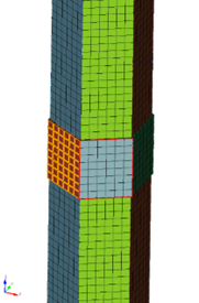
Figure 5: Example of duct 1 ACLP sidesets showing each face on the load pad is assigned to its own sideset.
[Contact]
  [aclp_1_3]
    primary = 'ACLP1_3'
    secondary = 'ACLP3_1'
    model = frictionless
    formulation = penalty
    normalize_penalty = true
    penalty = 1e10
    tangential_tolerance = 1.0e-3
    normal_smoothing_distance = 0.1
  []
  [aclp_3_10]
    primary = 'ACLP3_10'
    secondary = 'ACLP10_3'
    model = frictionless
    formulation = penalty
    normalize_penalty = true
    penalty = 1e10
    tangential_tolerance = 1.0e-3
    normal_smoothing_distance = 0.1
  []
  [aclp_3_11]
    primary = 'ACLP3_11'
    secondary = 'ACLP11_3'
    model = frictionless
    formulation = penalty
    normalize_penalty = true
    penalty = 1e10
    tangential_tolerance = 1.0e-3
    normal_smoothing_distance = 0.1
  []
  [tlp_1_3]
    primary = 'TLP1_3'
    secondary = 'TLP3_1'
    model = frictionless
    formulation = penalty
    normalize_penalty = true
    penalty = 1e10
    tangential_tolerance = 1.0e-3
    normal_smoothing_distance = 0.1
  []
  [tlp_3_10]
    primary = 'TLP3_10'
    secondary = 'TLP10_3'
    model = frictionless
    formulation = penalty
    normalize_penalty = true
    penalty = 1e10
    tangential_tolerance = 1.0e-3
    normal_smoothing_distance = 0.1
  []
  [tlp_3_11]
    primary = 'TLP3_11'
    secondary = 'TLP11_3'
    model = frictionless
    formulation = penalty
    normalize_penalty = true
    penalty = 1e10
    tangential_tolerance = 1.0e-3
    normal_smoothing_distance = 0.1
  []
[]Results
As a debugging check, the temperature calculated with the defined function is plotted in Figure 6 to ensure the temperatures have been correctly mapped to the duct. We can visually verify that the temperature below the active core region is 400°C, the temperature increases through the active core region, and above the active core the temperature on each side of the duct is held constant. The deformation output from the MOOSE simulation is also plotted in Figure 6. Duct 1 visibly bows from the high temperature side (bottom) towards the cooler temperature side (top) into the sector of ducts and contacts at the top of the duct.
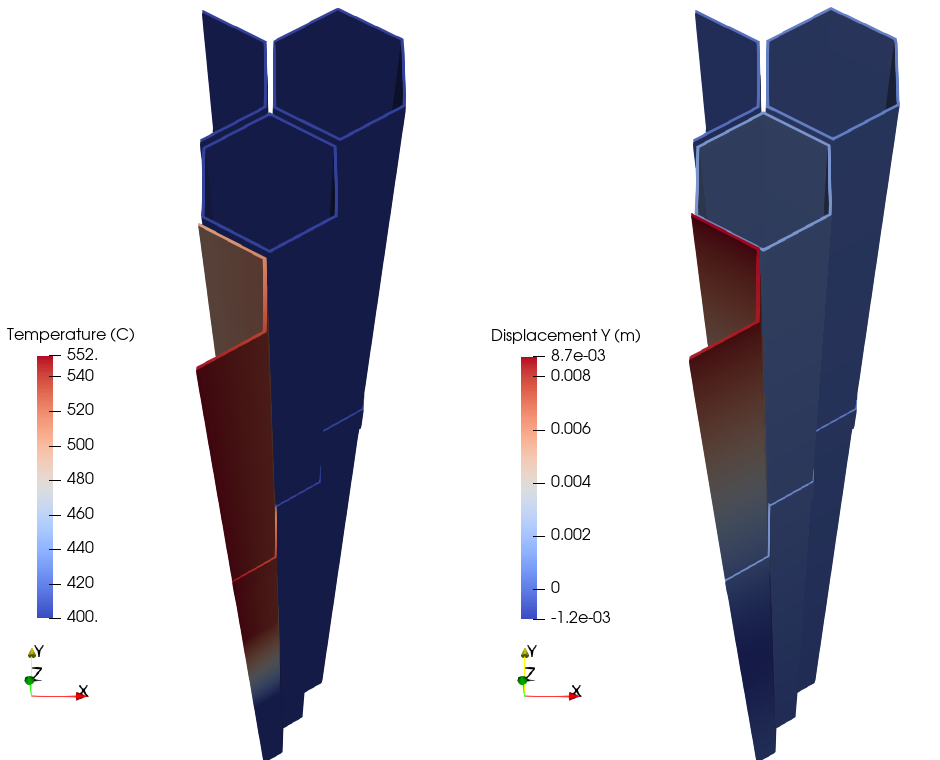
Figure 6: Temperature gradient mapping of the duct (left) and duct bowing (right).
Since MOOSE models only the duct walls, the centerline deformation of the duct is estimated by averaging the deformation of the flat faces at each axial height. The deformation from MOOSE simulation output for duct 1 is plotted in Figure 7 along with the calculation results from the participants from the IAEA report IAEA (1990) and agree well. A comparison of the deformation values at the core top, ACLP, and TLP are presented in Table 3, comparing the IAEA and MOOSE results. The values are all in good agreement, with MOOSE giving the maximum displacement of 8.59 mm at the TLP for duct 1 and the IAEA 8.54 mm. This benchmark verifies the MOOSE physics modules (Tensor Mechanics and Contact) for a small cluster of assemblies undergoing thermal bowing along the corner direction of the hexagonal assembly and contacting at load pads. Notable, reflective boundary conditions and a prior knowledge about which ducts would contact were used to substantially reduce the computational cost of the full sector problem.
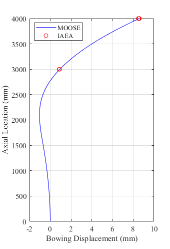
Figure 7: Duct bowing results for MOOSE calculations compared with closed-form solution results.
Table 3: Bowing results (in mm) at the top of the core, ACLP, and the TLP locations.
| Duct | IAEA | MOOSE |
|---|---|---|
| ACLP | ||
| 1 | 0.88 | 0.93 |
| 3 | 0.94 | 0.92 |
| 10 | 0.43 | 0.42 |
| TLP | ||
| 1 | 8.54 | 8.59 |
| 3 | 1.51 | 1.48 |
| 10 | 0.65 | 0.63 |
Run Command
This model requires the openly available Tensor Mechanics and Contact Modules which can be independently compiled from a MOOSE framework installation or leveraged from a MOOSE application which links to a version of MOOSE containing both these modules.
mpirun -np 20 /path/to/APP -i iaea_vp3a_symmetric_sector.i
References
- IAEA.
Verification and validation of lmfbr static core mechanics codes part i.
Technical Report IWGFR/75, International Atomic Energy Agency, 1990.[BibTeX]
- SNL.
CUBIT 15.5 User Documentation.
2019.[BibTeX]
- Nicholas Wozniak and Emily Shemon.
Continued Verification of MOOSE Structural Mechanics Tools for Modeling Core Bowing Phenomena in Fast Reactors.
Technical Report ANL/NSE-22/38, 1879091, 177085, Argonne National Laboratory, July 2022.
URL: https://www.osti.gov/servlets/purl/1879091/ (visited on 2022-09-16), doi:10.2172/1879091.[BibTeX]
- Nicholas Wozniak, Emily Shemon, James Grudzinski, and Benjamin Spencer.
Assessment of MOOSE-Based Tools for Calculating Radial Core Expansion.
Technical Report ANL/NSE-21/30, 1808314, 169472, Argonne National Laboratory, July 2021.
URL: https://www.osti.gov/servlets/purl/1808314/ (visited on 2022-03-16), doi:10.2172/1808314.[BibTeX]