Chapter 5: MultiApp Input Syntax & Examples

Principle & Syntax

The role of the MultiApps block in MOOSE is to allow the users to create vessels to contain any number of child applications. Important input parameters for the MultiApp block include app_type, which describes the child application to be invoked, and type, which describes the time/space-based execution of the child application. Various MultiApp types are available to facilitate different possible solution schemes of multi-physics problems. The input_files parameter is required for all types and it points to the child application input file. The remaining parameters in the MultiApp block will depend on the type. In the following sections, the app_type, type, and common parameters will be discussed.

Type of Child Application

The app_type parameter is the type of the child application to be executed. Child applications are MooseApp derived app or simply a physics module. Examples of app_type includes PronghornApp, GriffinApp, BisonApp, (MOOSE applications) as well as ReactorApp or TensorMechanicsApp (MOOSE physics modules). By default, the parent application is assumed to be capable of running the child applications so that no extra libraries need to be loaded. The user can alternatively provide a different application type for the child applications. In that case, the MOOSE application that runs the parent application will dynamically load the libraries that correspond to the specified app_type to run the child applications.

Type of MultiApp

The type parameter describes the time/space-based execution of the child application. Various MultiApp types are available to facilitate different possible solution schemes of multi-physics problems. Available types include: FullSolveMultiApp, TransientMultiApp, CentroidMultiApp, and several app types specific to the Stochastic Tools module (used for uncertainty quantification, parametric studies, meta-modeling and others).

FullSolveMultiApp

The FullSolveMultiApp object performs a complete child application simulation during each execution which means that the child applications will be solved from the first-time step to the last time step every time it is called. This is typically done for steady state or eigenvalue parent-app simulations or for initialization purposes.

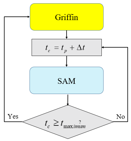
Figure 1: Example of FullSolveMultiApp.

Figure 1 shows an example of a FullSolveMultiApp where Griffin is the main application and SAM is the child application that will be solved throughout the entire time domain every time it is called. FullSolveMultiApp is generally used when we only need the end-time solution of the child application. In this example, the end-time SAM solution is used for the multiphysics coupling with a Griffin eigenvalue calculation.

TransientMultiApp

In the TransientMultiApp the child application will be solved at a single timestep, following the same timestep as the parent application. The child applications must use a transient Executioner. TransientMultiApp is used for performing coupled simulations with the parent and child application when both physics are marching in time together.

Figure 2: Example of Transientmultiapp.

Figure 2 shows an example of a TransientMultiApp where the main application (Griffin) and the child application (SAM) progress together in time. TransientMultiApp is simultaneously advancing the time-steps of the main and child applications by default. This means that no coupling fixed point iterations are done at any time-step. This approach is commonly referred to as loose coupling.

If a tight coupling approach is desired, Picard fixed point iterations may be used by specifying appropriate Executioner parameters for the parent application. Picard iterations are nonlinear iterations for tight coupling which repeat the simulation at the same time-step until a convergence criterion is satisfied. Picard iterations are particularly important if the physics solved in the different apps have very strong nonlinear effects.

The following two examples describe the use of the TransientMultiApp. The definitions of execute_on and positions will be given in the optional parameters.

[MultiApps]
  [dynamic_executable]
    type = TransientMultiApp
    execute_on = 'TIMESTEP_END'
    input_files = 'pebble.i'
  []
[]

[MultiApps]
 [sub]
    type = TransientMultiApp
    app_type = BisonApp
    input_files = 'Bison_input.i'
    positions = '0   0   0
                 0.5 0.5 0
                 0.9 0.9 0'
  []
[]

The minimum time step over the main and all child applications will be used, by default, unless sub_cycling is enabled. If sub_cycling is enabled this will allow faster calculations, as the parent app will not be forced to use the smaller time step from the child app.

CentroidMultiApp

CentroidMultiApp is used to allow a child application to be launched in space at the centroid of every element in the parent application. This option can be leveraged when multiscale solves are desired. This object requires no special parameters. The child applications can optionally be restricted to solve only on specified blocks (subdomains) by using the CentroidMultiApp.

[MultiApps]
  [sub]
    type = CentroidMultiApp
    app_type = GriffinApp
    input_files = 'Griffin_input.i'
  []
[]

MultiApp Classes in `Stochastic Tools App`

The Stochastic Tools module is a toolbox designed for performing stochastic analysis for MOOSE-based applications. It can be used as a parent application to statistically control some key parameters in other MOOSE applications as its child applications.

The Stochastic Tools apps include SamplerFullSolveMultiApp , `SamplerTransientMultiApp ` , and PODFullSolveMultiApp . SamplerFullSolveMultiApp and `SamplerTransientMultiApp ` create full solve type, and transient type child application, respectively.

Required Parameters

Input Files

The input_files parameter is required regardless of MultiApp type. The input_files parameter specifies the input file for the child application. If the positions parameter is used to specify multiple instances of the child application at different locations in the domain, the same input file will be used at each position. It is possible to specify different input files at each position. Meanwhile, if the user has N points specified by either positions or positions_file, the can provide an array of N input file names for input_files. The ith input file name will be used to run the child application at the $var element = document.getElementById("moose-equation-9df14071-c533-400e-a4fd-ab410e92c145");katex.render("i^{th}", element, {displayMode:false,throwOnError:false});$ position. In the example below, the input file (name.i) will be used for all the child applications within the MultiApps block named "micro".

[MultiApps]
  [micro]
    type = TransientMultiApp
    app_type  = BisonApp
    positions =   '0.01285  0.0       0
                   0.01285  0.0608    0
                   0.01285  0. 1216   0
                   0.01285  0.1824    0'
    input_files = name.i
    execute_on = 'timestep_end'
  []
[]

Optional Parameters

Timing of Execution

The execute_on parameter specifies when a child application is to be executed, in relation to the parent application timesteps. The most common options are to execute the child application at the beginning of the time step, at the end of the time step, or at the initial condition of the entire simulation. By default, child application execution will occur at the beginning of time-step. In the previous example, at every time step, the main application will be executed first, then the child applications will be executed at the end of the time step. Some common options of execute_on are summarized below:

1. TIMESTEP_BEGIN: Launch child application at the beginning of the time step

2. TIMESTEP_END: Launch child application at the end of the time step

3. INITIAL: Launch child application only at the initial condition to set up the initial conditions for the solve

4. NONLINEAR: This option has limited applications and is used to inject the coupling information into the middle of the Newton solve. It will likely slow down the newton convergence, as the contribution to the Jacobian are not considered, but could speed up the convergence of the entire system.

Finer Timesteps in Child Applications

Applications may use different time step sizes by allowing subcycling. The subcycling option is useful for allowing different timescales. For instance, a relatively slow physics application may use bigger time steps (e.g. 10 sec) whereas a rapidly changing physics may use relatively small-time step (e.g. 0.1 sec). Thus, the first app takes one time-step of 10 sec while the other app takes 100 time-steps of 0.1 sec to reach the same end time as the first application.

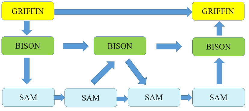
Figure 3: Schematic drawing of the sub-cycling concept.

Figure 3 illustrates a transient Multiphysics simulation in which Griffin, Bison, and SAM are coupled at different timescales using the subcycling option. When performing sub-cycling, transferred auxiliary variables on child applications may be interpolated between the start time and the end time of the main app with the interpolate_transfers parameter. When using the TransientMultiApp type, the sub_cycling parameter can be used to invoke subcycling.

Locations of Child Applications

Child applications can be launched at various spatial positions of the parent application geometry by using the 'positions' input parameter. Positions are simply a list of 3D coordinates that describe the offset of the child application's origin from the parent application's origin. If no positions are provided, the child application will be launched at the position 0 0 0 within the parent application. Notice that in the example below, the number of child applications to be invoked is not explicitly defined but rather is inferred from the number of positions given. The example shows five different positions, thus, five independent versions of the child application BisonApp will be created and each of them will be associated with a different position within the parent application domain. The user may also provide a position file instead of explicitly providing the positions in the MultiApp block; this feature is useful when the user wants to invoke thousands of child application as the separate input file can contain all this information without cluttering the main input file. A common use of positions in nuclear reactor analysis is the launching of individual fuel rod (BISON) simulations at various fuel rods within a reactor assembly or core.

[MultiApps]
  [micor]
    type = TransientMultiApp
    app_type  = BisonApp
    positions =   '0.013  0    0
                   0.013  0.09    0
                   0.013  0. 18   0
                   0.013  0.27    0'
                   0.013  0.36    0'
    input_files = name.i
    execute_on = 'timestep_end'
  []
[]

The user may also provide positions in a "position file" rather than in the the MultiApp block. This is useful when the number of positions is exceedingly large. For example, the heat-pipe cooled microreactor example demonstrates the use of the positions file to invoke Sockeye heat pipe temperatures calculations on each heat pipe in the domain.

[MultiApps]
  [sockeye]
    type = TransientMultiApp
    positions_file = 'hp_centers.txt'
    input_files = 'MP_FC_ss_sockeye.i'
    execute_on = 'timestep_begin' # execute on timestep begin because hard to have a good initial guess on heat flux
    max_procs_per_app = 1
    output_in_position = true
  []
[]

The list and location of each heat-pipe are provided in hp_centers.txt as follows:

0.133760510365853 0.369680000000000 0.000000000000000
0.173597678939937 0.346680000000000 0.000000000000000
0.213434847514021 0.323680000000000 0.000000000000000
0.253272016088105 0.300680000000000 0.000000000000000
0.0939233417917683 0.346680000000000 0.000000000000000
0.133760510365853 0.323680000000000 0.000000000000000
0.173597678939937 0.300680000000000 0.000000000000000
0.213434847514021 0.277680000000000 0.000000000000000
0.253272016088105 0.254680000000000 0.000000000000000
0.0540861732176842 0.323680000000000 0.000000000000000
0.0939233417917683 0.300680000000000 0.000000000000000
0.133760510365853 0.277680000000000 0.000000000000000
0.173597678939937 0.254680000000000 0.000000000000000
0.213434847514021 0.231680000000000 0.000000000000000
0.253272016088105 0.208680000000000 0.000000000000000
0.0142490046436000 0.300680000000000 0.000000000000000
0.0540861732176842 0.277680000000000 0.000000000000000
0.0939233417917683 0.254680000000000 0.000000000000000
0.133760510365853 0.231680000000000 0.000000000000000
0.173597678939937 0.208680000000000 0.000000000000000
0.213434847514021 0.185680000000000 0.000000000000000
0.253272016088105 0.162680000000000 0.000000000000000
0.0142490046436000 0.254680000000000 0.000000000000000
0.0540861732176842 0.231680000000000 0.000000000000000
0.0939233417917683 0.208680000000000 0.000000000000000
0.133760510365853 0.185680000000000 0.000000000000000
0.173597678939937 0.162680000000000 0.000000000000000
0.213434847514021 0.139680000000000 0.000000000000000
0.0142490046436000 0.208680000000000 0.000000000000000
0.0540861732176842 0.185680000000000 0.000000000000000
0.0939233417917683 0.162680000000000 0.000000000000000
0.133760510365853 0.139680000000000 0.000000000000000
0.173597678939937 0.116680000000000 0.000000000000000
0.0142490046436000 0.162680000000000 0.000000000000000
0.0540861732176842 0.139680000000000 0.000000000000000
0.0939233417917684 0.116680000000000 0.000000000000000
0.133760510365853 0.0936800000000000 0.000000000000000
0.267521020731705 0.601360000000000 0.000000000000000
0.307358189305789 0.578360000000000 0.000000000000000
0.347195357879873 0.555360000000000 0.000000000000000
0.387032526453958 0.532360000000000 0.000000000000000
0.227683852157621 0.578360000000000 0.000000000000000
0.267521020731705 0.555360000000000 0.000000000000000
0.307358189305789 0.532360000000000 0.000000000000000
0.347195357879873 0.509360000000000 0.000000000000000
0.387032526453958 0.486360000000000 0.000000000000000
0.187846683583537 0.555360000000000 0.000000000000000
0.227683852157621 0.532360000000000 0.000000000000000
0.267521020731705 0.509360000000000 0.000000000000000
0.307358189305789 0.486360000000000 0.000000000000000
0.347195357879873 0.463360000000000 0.000000000000000
0.387032526453958 0.440360000000000 0.000000000000000
0.148009515009453 0.532360000000000 0.000000000000000
0.187846683583537 0.509360000000000 0.000000000000000
0.227683852157621 0.486360000000000 0.000000000000000
0.267521020731705 0.463360000000000 0.000000000000000
0.307358189305789 0.440360000000000 0.000000000000000
0.347195357879873 0.417360000000000 0.000000000000000
0.387032526453958 0.394360000000000 0.000000000000000
0.148009515009453 0.486360000000000 0.000000000000000
0.187846683583537 0.463360000000000 0.000000000000000
0.227683852157621 0.440360000000000 0.000000000000000
0.267521020731705 0.417360000000000 0.000000000000000
0.307358189305789 0.394360000000000 0.000000000000000
0.347195357879873 0.371360000000000 0.000000000000000
0.148009515009453 0.440360000000000 0.000000000000000
0.187846683583537 0.417360000000000 0.000000000000000
0.227683852157621 0.394360000000000 0.000000000000000
0.267521020731705 0.371360000000000 0.000000000000000
0.307358189305789 0.348360000000000 0.000000000000000
0.148009515009453 0.394360000000000 0.000000000000000
0.187846683583537 0.371360000000000 0.000000000000000
0.227683852157621 0.348360000000000 0.000000000000000
0.267521020731705 0.325360000000000 0.000000000000000
0 0.601360000000000 0.000000000000000
0.0398371685740842 0.578360000000000 0.000000000000000
0.0796743371481683 0.555360000000000 0.000000000000000
0.119511505722252 0.532360000000000 0.000000000000000
0 0.555360000000000 0.000000000000000
0.0398371685740842 0.532360000000000 0.000000000000000
0.0796743371481684 0.509360000000000 0.000000000000000
0.119511505722252 0.486360000000000 0.000000000000000
0 0.509360000000000 0.000000000000000
0.0398371685740842 0.486360000000000 0.000000000000000
0.0796743371481684 0.463360000000000 0.000000000000000
0.119511505722252 0.440360000000000 0.000000000000000
0 0.463360000000000 0.000000000000000
0.0398371685740842 0.440360000000000 0.000000000000000
0.0796743371481684 0.417360000000000 0.000000000000000
0.119511505722252 0.394360000000000 0.000000000000000
0 0.417360000000000 0.000000000000000
0.0398371685740842 0.394360000000000 0.000000000000000
0.0796743371481684 0.371360000000000 0.000000000000000
0 0.371360000000000 0.000000000000000
0.0398371685740842 0.348360000000000 0.000000000000000
0 0.325360000000000 0.000000000000000
0.133760510365853 0.833040000000000 0.000000000000000
0.173597678939937 0.810040000000000 0.000000000000000
0.213434847514021 0.787040000000000 0.000000000000000
0.253272016088105 0.764040000000000 0.000000000000000
0.0939233417917683 0.810040000000000 0.000000000000000
0.133760510365853 0.787040000000000 0.000000000000000
0.173597678939937 0.764040000000000 0.000000000000000
0.213434847514021 0.741040000000000 0.000000000000000
0.253272016088105 0.718040000000000 0.000000000000000
0.0540861732176841 0.787040000000000 0.000000000000000
0.0939233417917683 0.764040000000000 0.000000000000000
0.133760510365853 0.741040000000000 0.000000000000000
0.173597678939937 0.718040000000000 0.000000000000000
0.213434847514021 0.695040000000000 0.000000000000000
0.253272016088105 0.672040000000000 0.000000000000000
0.0142490046436000 0.764040000000000 0.000000000000000
0.0540861732176841 0.741040000000000 0.000000000000000
0.0939233417917683 0.718040000000000 0.000000000000000
0.133760510365853 0.695040000000000 0.000000000000000
0.173597678939937 0.672040000000000 0.000000000000000
0.213434847514021 0.649040000000000 0.000000000000000
0.253272016088105 0.626040000000000 0.000000000000000
0.0142490046436000 0.718040000000000 0.000000000000000
0.0540861732176841 0.695040000000000 0.000000000000000
0.0939233417917683 0.672040000000000 0.000000000000000
0.133760510365853 0.649040000000000 0.000000000000000
0.173597678939937 0.626040000000000 0.000000000000000
0.213434847514021 0.603040000000000 0.000000000000000
0.0142490046436000 0.672040000000000 0.000000000000000
0.0540861732176841 0.649040000000000 0.000000000000000
0.0939233417917683 0.626040000000000 0.000000000000000
0.133760510365853 0.603040000000000 0.000000000000000
0.173597678939937 0.580040000000000 0.000000000000000
0.0142490046436000 0.626040000000000 0.000000000000000
0.0540861732176841 0.603040000000000 0.000000000000000
0.0939233417917683 0.580040000000000 0.000000000000000
0.133760510365853 0.557040000000000 0.000000000000000
0.401281531097558 0.369680000000000 0.000000000000000
0.441118699671642 0.346680000000000 0.000000000000000
0.480955868245726 0.323680000000000 0.000000000000000
0.520793036819810 0.300680000000000 0.000000000000000
0.361444362523473 0.346680000000000 0.000000000000000
0.401281531097558 0.323680000000000 0.000000000000000
0.441118699671642 0.300680000000000 0.000000000000000
0.480955868245726 0.277680000000000 0.000000000000000
0.321607193949389 0.323680000000000 0.000000000000000
0.361444362523473 0.300680000000000 0.000000000000000
0.401281531097558 0.277680000000000 0.000000000000000
0.441118699671642 0.254680000000000 0.000000000000000
0.281770025375305 0.300680000000000 0.000000000000000
0.321607193949389 0.277680000000000 0.000000000000000
0.361444362523473 0.254680000000000 0.000000000000000
0.401281531097558 0.231680000000000 0.000000000000000
0.281770025375305 0.254680000000000 0.000000000000000
0.321607193949389 0.231680000000000 0.000000000000000
0.361444362523473 0.208680000000000 0.000000000000000
0.281770025375305 0.208680000000000 0.000000000000000
0.321607193949389 0.185680000000000 0.000000000000000
0.281770025375305 0.162680000000000 0.000000000000000
0.535042041463410 0.601360000000000 0.000000000000000
0.574879210037494 0.578360000000000 0.000000000000000
0.614716378611578 0.555360000000000 0.000000000000000
0.654553547185663 0.532360000000000 0.000000000000000
0.495204872889326 0.578360000000000 0.000000000000000
0.535042041463410 0.555360000000000 0.000000000000000
0.574879210037494 0.532360000000000 0.000000000000000
0.614716378611579 0.509360000000000 0.000000000000000
0.654553547185663 0.486360000000000 0.000000000000000
0.455367704315242 0.555360000000000 0.000000000000000
0.495204872889326 0.532360000000000 0.000000000000000
0.535042041463410 0.509360000000000 0.000000000000000
0.574879210037494 0.486360000000000 0.000000000000000
0.614716378611579 0.463360000000000 0.000000000000000
0.654553547185663 0.440360000000000 0.000000000000000
0.415530535741158 0.532360000000000 0.000000000000000
0.455367704315242 0.509360000000000 0.000000000000000
0.495204872889326 0.486360000000000 0.000000000000000
0.535042041463410 0.463360000000000 0.000000000000000
0.574879210037494 0.440360000000000 0.000000000000000
0.614716378611579 0.417360000000000 0.000000000000000
0.654553547185663 0.394360000000000 0.000000000000000
0.415530535741158 0.486360000000000 0.000000000000000
0.455367704315242 0.463360000000000 0.000000000000000
0.495204872889326 0.440360000000000 0.000000000000000
0.535042041463410 0.417360000000000 0.000000000000000
0.574879210037494 0.394360000000000 0.000000000000000
0.614716378611579 0.371360000000000 0.000000000000000
0.415530535741158 0.440360000000000 0.000000000000000
0.455367704315242 0.417360000000000 0.000000000000000
0.495204872889326 0.394360000000000 0.000000000000000
0.535042041463410 0.371360000000000 0.000000000000000
0.574879210037494 0.348360000000000 0.000000000000000
0.415530535741158 0.394360000000000 0.000000000000000
0.455367704315242 0.371360000000000 0.000000000000000
0.495204872889326 0.348360000000000 0.000000000000000
0.535042041463410 0.325360000000000 0.000000000000000

Parallel Options

When the mesh requires large memory usage, it is useful to use Distributed Mesh by setting parallel_type as distributed in the Mesh block so that the different portions can be stored in different processors.

It is also useful to assign a few processors for small or memory-intensive solves using max_procs_per_app which is the maximum number of processors to give to each App. However, for large solves, the user can assign the minimum number of processors to give to each App using min_procs_per_app.

Other Options

For the MOOSE Apps: FullSolveMultiApp, TransientMultiApp, and CentroidMultiApp. There are various common optional parameters such as app_type, bounding_box_inflation, bounding_box_padding, catch_up, cli_args, cli_args_files , clone_master_mesh , detect_steady_state, global_time_offset , keep_solution_during_restore, library_name, library_path,output_in_position, and execute_on.

Other parameters are allowed only for specific MultiApps type. For example, positions is an optional parameter for FullSolveMultiApp and TransientMultiApp, but it is not a parameter for CentroidMultiApp. Generally, these optional parameters were developed to facilitate flexible multi-physics simulations. The no_restore optional parameter is useful when doing steady-state Picard iterations where we want to use the solution of previous Picard iteration as the initial guess of the current Picard iteration.

In addittion, if the user wants to pass additional command line argument to the sub apps this can be done using cli_args, or the file names that should be looked in for additional command line arguments to pass to the sub apps can be defined using cli_args_files.

Mesh Displacement

There are different mesh options that are available in MOOSE. Calculations can be performed on the initial mesh configuration or, when requested, a displaced mesh configuration. To enable displacements, provide a vector of displacement variable names for each spatial dimension in the displacements parameters within the Mesh block. Once enabled, any object that should operate on the displaced configuration should set the use_displaced_mesh to true. For example, the following snippet enables the computation of a Postprocessor with and without the displaced configuration.

[Mesh]
  type = FileMesh
  file = truss_2d.e
  displacements = 'disp_x disp_y'
[]

[Postprocessors]
  [without]
    type = ElementIntegralVariablePostprocessor
    variable = c
    execute_on = initial
  []
  [with]
    type = ElementIntegralVariablePostprocessor
    variable = c
    use_displaced_mesh = true
    execute_on = initial
  []
[]

If the child application uses the same mesh as the parent application, the clone_master_mesh parameter allows for re-using the main application mesh in the child application.

Restart and Recovery

Restart/Recover is useful to restart a simulation using data from a previous simulation. If the same mesh file will be used, and the initial conditions need to be varied, the user can use Variable Initialization. Nevertheless, for the other situations, checkpoint files will be needed. The checkpoint files will include all the simulation information, including those of all the child and grandchild applications (infinite recursion), that are needed for advanced restart of the simulation. The following block should be added to the input file to create the checkpoint files.

[Outputs]
  checkpoint = true
[]

It should be noticed that enabling the checkpoint for the parent application will store all the required information to restart the data from all child applications. If a simulation is terminated by mistake, the user can recover the simulation using --recover command-line flag if checkpoint files were enabled.

Go to Chapter 6

(microreactors/mrad/legacy/steady/MP_FC_ss_bison.i)

################################################################################
## NEAMS Micro-Reactor Application Driver                                     ##
## BISON Main Application input file                                          ##
## Thermal (Heat Conduction) model only                                       ##
## Constant and uniform power profile in fuel region                          ##
## POC: Nicholas Stauff, nstauff at anl.gov                                   ##
################################################################################
# If using or referring to this model, please cite as explained in
# https://mooseframework.inl.gov/virtual_test_bed/citing.html

[GlobalParams]
  flux_conversion_factor = 1
[]

# Note: the mesh is stored using git large file system (LFS)
[Mesh]
  file = ../mesh/mrad_mesh.e
[]

[Variables]
  [temp]
    initial_condition = 800
  []
[]

[Kernels]
  [heat_conduction]
    type = HeatConduction
    variable = temp
  []
  [heat_ie]
    type = HeatConductionTimeDerivative
    variable = temp
  []
  [heat_source_fuel]
    type = CoupledForce
    variable = temp
    block = fuel
    v = power_density
  []
  [heat_sink_center_comp]
    type = CoupledForce
    variable = temp
    block = heat_pipes
    v = hp_flux_aux
  []
[]

[AuxVariables]
  [power_density]
    block = fuel
    family = L2_LAGRANGE
    order = FIRST
    initial_condition = 3.4e6
  []
  [Tfuel]
    block = fuel
  []
  [fuel_thermal_conductivity]
    block = fuel
    order = CONSTANT
    family = MONOMIAL
  []
  [fuel_specific_heat]
    block = fuel
    order = CONSTANT
    family = MONOMIAL
  []
  [monolith_thermal_conductivity]
    block = 'monolith '
    order = CONSTANT
    family = MONOMIAL
  []
  [monolith_specific_heat]
    block = 'monolith '
    order = CONSTANT
    family = MONOMIAL
  []
  [temp_uo] #auxvariable to hold heat pipe surface temperature from UserObject
    initial_condition = 800
    block = 'heat_pipes'
  []
  [hp_flux_aux]
    block = 'heat_pipes'
  []
[]

[AuxKernels]
  [assign_tfuel]
    type = NormalizationAux
    variable = Tfuel
    source_variable = temp
    execute_on = 'timestep_end'
  []
  [fuel_thermal_conductivity]
    type = MaterialRealAux
    variable = fuel_thermal_conductivity
    property = thermal_conductivity
    execute_on = timestep_end
  []
  [fuel_specific_heat]
    type = MaterialRealAux
    variable = fuel_specific_heat
    property = specific_heat
    execute_on = timestep_end
  []
  [monolith_thermal_conductivity]
    type = MaterialRealAux
    variable = monolith_thermal_conductivity
    property = thermal_conductivity
    execute_on = timestep_end
  []
  [monolith_specific_heat]
    type = MaterialRealAux
    variable = monolith_specific_heat
    property = specific_heat
    execute_on = timestep_end
  []
  [temp_uo]
    type = SpatialUserObjectAux
    variable = temp_uo
    user_object = temp_uo
  []
[]

[BCs]
  [outside_bc] # An "inefficient" cooling mechanism through outer surfaces
    type = ConvectiveFluxFunction # (Robin BC)
    variable = temp
    boundary = 'reflector_surface_all B4C_surface_all air_surface_all'
    coefficient = 1e3 # W/K/m^2
    T_infinity = 800 # K air temperature at the top of the core
  []
[]

[Materials]
  [fuel_matrix_thermal]
    type = GraphiteMatrixThermal
    block = fuel
    packing_fraction = 0.4
    specific_heat_scale_factor = 1.0
    thermal_conductivity_scale_factor = 1.0
    graphite_grade = IG_110
    fast_neutron_fluence = 0 # Fresh matrix (near BoC)
    temperature = temp
  []
  [monolith_matrix_thermal]
    type = GraphiteMatrixThermal
    block = 'monolith '
    packing_fraction = 0
    specific_heat_scale_factor = 1.0
    thermal_conductivity_scale_factor = 1.0
    graphite_grade = IG_110
    fast_neutron_fluence = 0 # Fresh matrix (near BoC)
    temperature = temp
  []
  [moderator_thermal]
    type = HeatConductionMaterial
    block = moderator
    temp = temp
    thermal_conductivity = 20 # W/m/K
    specific_heat = 500 # arbitrary value
  []
  [heat_pipes_thermal]
    type = HeatConductionMaterial
    block = 'heat_pipes' # Vapor with high thermal conductivity
    temp = temp
    thermal_conductivity = 1e4 # W/m/K
    specific_heat = 5 # arbitrary value
  []
  [airgap_thermal]
    type = HeatConductionMaterial
    block = 'air_gap' # Helium gap
    temp = temp
    thermal_conductivity = 0.15 # W/m/K
    specific_heat = 5197 # arbitrary value
  []
  [axial_reflector_thermal]
    type = HeatConductionMaterial
    block = 'reflector'
    temp = temp
    thermal_conductivity = 199 # W/m/K
    specific_heat = 1867 # arbitrary value
  []
  [B4C_thermal]
    type = HeatConductionMaterial
    block = 'B4C'
    temp = temp
    thermal_conductivity = 92 # W/m/K
    specific_heat = 960 # arbitrary value
  []
  [fuel_density]
    type = Density
    block = fuel
    density = 2276.5
  []
  [moderator_density]
    type = Density
    block = moderator
    density = 4.3e3
  []
  [monolith_density]
    type = Density
    block = 'monolith'
    density = 1806
  []
  [heat_pipes_density]
    type = Density
    block = 'heat_pipes'
    density = 180 #random number for vapor
  []
  [airgap_density]
    type = Density
    block = air_gap #helium
    density = 180
  []
  [axial_reflector_density]
    type = Density
    block = reflector
    density = 1848
  []
  [B4C_density]
    type = Density
    block = B4C
    density = 2510
  []
[]

[MultiApps]
  [sockeye]
    type = TransientMultiApp
    positions_file = 'hp_centers.txt'
    input_files = 'MP_FC_ss_sockeye.i'
    execute_on = 'timestep_begin' # execute on timestep begin because hard to have a good initial guess on heat flux
    max_procs_per_app = 1
    output_in_position = true
  []
[]

[Transfers]
  [from_sockeye_flux] # Transfer heat pipe heat flux from Sockeye subapps
    type = MultiAppGeneralFieldNearestLocationTransfer
    from_multi_app = sockeye
    source_variable = flux_uo
    variable = hp_flux_aux
    execute_on = 'timestep_begin'
    # Reduces transfers efficiency for now, can be removed once transferred fields are checked
    bbox_factor = 10
  []
  [to_sockeye_temp] # Transfer heat pipe surface temperature to Sockeye subapps
    type = MultiAppGeneralFieldNearestLocationTransfer
    to_multi_app = sockeye
    source_variable = temp_uo
    variable = T_wall_var
    execute_on = 'timestep_begin'
    # Reduces transfers efficiency for now, can be removed once transferred fields are checked
    bbox_factor = 10
  []
[]

[UserObjects]
  [temp_uo]
    type = NearestPointLayeredSideAverage
    direction = z
    num_layers = 100
    points_file = 'hp_centers.txt'
    variable = temp
    execute_on = linear
    boundary = 'heat_pipe_boundary_up_side heat_pipe_boundary_core_side'
  []
[]

[Executioner]
  type = Transient

  petsc_options_iname = '-pc_type -pc_factor_mat_solver_package -ksp_gmres_restart'
  petsc_options_value = 'lu       superlu_dist                  51'
  line_search = 'none'

  nl_rel_tol = 1e-7
  nl_abs_tol = 1e-8

  start_time = -2e4 # negative start time so we can start running from t = 0
  end_time = 0
  dtmin = 1
  dt = 50

  # Time integration scheme
  scheme = 'implicit-euler'
[]

[Postprocessors]
  [total_evap_heat_exam]
    type = ElementIntegralVariablePostprocessor
    variable = hp_flux_aux
    block = 'heat_pipes'
    execute_on = 'initial timestep_end'
  []
  [hp_heat_integral]
    type = SideDiffusiveFluxIntegral
    variable = temp
    boundary = 'heat_pipe_boundary_up_side heat_pipe_boundary_core_side'
    diffusivity = thermal_conductivity
    execute_on = 'initial timestep_end'
  []
  [fuel_temp_avg]
    type = ElementAverageValue
    variable = temp
    block = fuel
  []
  [fuel_temp_max]
    type = ElementExtremeValue
    variable = temp
    block = fuel
  []
  [fuel_temp_min]
    type = ElementExtremeValue
    variable = temp
    block = fuel
    value_type = min
  []
  [mod_temp_avg]
    type = ElementAverageValue
    variable = temp
    block = moderator
  []
  [mod_temp_max]
    type = ElementExtremeValue
    variable = temp
    block = moderator
  []
  [mod_temp_min]
    type = ElementExtremeValue
    variable = temp
    block = moderator
    value_type = min
  []
  [monolith_temp_avg]
    type = ElementAverageValue
    variable = temp
    block = monolith
  []
  [monolith_temp_max]
    type = ElementExtremeValue
    variable = temp
    block = monolith
  []
  [monolith_temp_min]
    type = ElementExtremeValue
    variable = temp
    block = monolith
    value_type = min
  []
  [heatpipe_surface_temp_avg]
    type = SideAverageValue
    variable = temp
    boundary = heat_pipe_boundary_all
  []
  [power_density]
    type = ElementIntegralVariablePostprocessor
    block = fuel
    variable = power_density
    execute_on = 'initial timestep_end'
  []
  [fuel_cP]
    type = ElementExtremeValue
    value_type = 'max'
    variable = fuel_specific_heat
    block = fuel
    execute_on = 'initial timestep_end'
  []
  [fuel_k]
    type = ElementExtremeValue
    value_type = 'max'
    variable = fuel_thermal_conductivity
    block = fuel
    execute_on = 'initial timestep_end'
  []
  [monolith_cP]
    type = ElementExtremeValue
    value_type = 'max'
    variable = monolith_specific_heat
    block = 'monolith '
    execute_on = 'initial timestep_end'
  []
  [monolith_k]
    type = ElementExtremeValue
    value_type = 'max'
    variable = monolith_thermal_conductivity
    block = 'monolith '
    execute_on = 'initial timestep_end'
  []
[]

[Outputs]
  perf_graph = true
  exodus = true
  color = true
  csv = false
  #checkpoint = true
[]

(microreactors/mrad/legacy/steady/hp_centers.txt)

0.133760510365853 0.369680000000000 0.000000000000000
0.173597678939937 0.346680000000000 0.000000000000000
0.213434847514021 0.323680000000000 0.000000000000000
0.253272016088105 0.300680000000000 0.000000000000000
0.0939233417917683 0.346680000000000 0.000000000000000
0.133760510365853 0.323680000000000 0.000000000000000
0.173597678939937 0.300680000000000 0.000000000000000
0.213434847514021 0.277680000000000 0.000000000000000
0.253272016088105 0.254680000000000 0.000000000000000
0.0540861732176842 0.323680000000000 0.000000000000000
0.0939233417917683 0.300680000000000 0.000000000000000
0.133760510365853 0.277680000000000 0.000000000000000
0.173597678939937 0.254680000000000 0.000000000000000
0.213434847514021 0.231680000000000 0.000000000000000
0.253272016088105 0.208680000000000 0.000000000000000
0.0142490046436000 0.300680000000000 0.000000000000000
0.0540861732176842 0.277680000000000 0.000000000000000
0.0939233417917683 0.254680000000000 0.000000000000000
0.133760510365853 0.231680000000000 0.000000000000000
0.173597678939937 0.208680000000000 0.000000000000000
0.213434847514021 0.185680000000000 0.000000000000000
0.253272016088105 0.162680000000000 0.000000000000000
0.0142490046436000 0.254680000000000 0.000000000000000
0.0540861732176842 0.231680000000000 0.000000000000000
0.0939233417917683 0.208680000000000 0.000000000000000
0.133760510365853 0.185680000000000 0.000000000000000
0.173597678939937 0.162680000000000 0.000000000000000
0.213434847514021 0.139680000000000 0.000000000000000
0.0142490046436000 0.208680000000000 0.000000000000000
0.0540861732176842 0.185680000000000 0.000000000000000
0.0939233417917683 0.162680000000000 0.000000000000000
0.133760510365853 0.139680000000000 0.000000000000000
0.173597678939937 0.116680000000000 0.000000000000000
0.0142490046436000 0.162680000000000 0.000000000000000
0.0540861732176842 0.139680000000000 0.000000000000000
0.0939233417917684 0.116680000000000 0.000000000000000
0.133760510365853 0.0936800000000000 0.000000000000000
0.267521020731705 0.601360000000000 0.000000000000000
0.307358189305789 0.578360000000000 0.000000000000000
0.347195357879873 0.555360000000000 0.000000000000000
0.387032526453958 0.532360000000000 0.000000000000000
0.227683852157621 0.578360000000000 0.000000000000000
0.267521020731705 0.555360000000000 0.000000000000000
0.307358189305789 0.532360000000000 0.000000000000000
0.347195357879873 0.509360000000000 0.000000000000000
0.387032526453958 0.486360000000000 0.000000000000000
0.187846683583537 0.555360000000000 0.000000000000000
0.227683852157621 0.532360000000000 0.000000000000000
0.267521020731705 0.509360000000000 0.000000000000000
0.307358189305789 0.486360000000000 0.000000000000000
0.347195357879873 0.463360000000000 0.000000000000000
0.387032526453958 0.440360000000000 0.000000000000000
0.148009515009453 0.532360000000000 0.000000000000000
0.187846683583537 0.509360000000000 0.000000000000000
0.227683852157621 0.486360000000000 0.000000000000000
0.267521020731705 0.463360000000000 0.000000000000000
0.307358189305789 0.440360000000000 0.000000000000000
0.347195357879873 0.417360000000000 0.000000000000000
0.387032526453958 0.394360000000000 0.000000000000000
0.148009515009453 0.486360000000000 0.000000000000000
0.187846683583537 0.463360000000000 0.000000000000000
0.227683852157621 0.440360000000000 0.000000000000000
0.267521020731705 0.417360000000000 0.000000000000000
0.307358189305789 0.394360000000000 0.000000000000000
0.347195357879873 0.371360000000000 0.000000000000000
0.148009515009453 0.440360000000000 0.000000000000000
0.187846683583537 0.417360000000000 0.000000000000000
0.227683852157621 0.394360000000000 0.000000000000000
0.267521020731705 0.371360000000000 0.000000000000000
0.307358189305789 0.348360000000000 0.000000000000000
0.148009515009453 0.394360000000000 0.000000000000000
0.187846683583537 0.371360000000000 0.000000000000000
0.227683852157621 0.348360000000000 0.000000000000000
0.267521020731705 0.325360000000000 0.000000000000000
0 0.601360000000000 0.000000000000000
0.0398371685740842 0.578360000000000 0.000000000000000
0.0796743371481683 0.555360000000000 0.000000000000000
0.119511505722252 0.532360000000000 0.000000000000000
0 0.555360000000000 0.000000000000000
0.0398371685740842 0.532360000000000 0.000000000000000
0.0796743371481684 0.509360000000000 0.000000000000000
0.119511505722252 0.486360000000000 0.000000000000000
0 0.509360000000000 0.000000000000000
0.0398371685740842 0.486360000000000 0.000000000000000
0.0796743371481684 0.463360000000000 0.000000000000000
0.119511505722252 0.440360000000000 0.000000000000000
0 0.463360000000000 0.000000000000000
0.0398371685740842 0.440360000000000 0.000000000000000
0.0796743371481684 0.417360000000000 0.000000000000000
0.119511505722252 0.394360000000000 0.000000000000000
0 0.417360000000000 0.000000000000000
0.0398371685740842 0.394360000000000 0.000000000000000
0.0796743371481684 0.371360000000000 0.000000000000000
0 0.371360000000000 0.000000000000000
0.0398371685740842 0.348360000000000 0.000000000000000
0 0.325360000000000 0.000000000000000
0.133760510365853 0.833040000000000 0.000000000000000
0.173597678939937 0.810040000000000 0.000000000000000
0.213434847514021 0.787040000000000 0.000000000000000
0.253272016088105 0.764040000000000 0.000000000000000
0.0939233417917683 0.810040000000000 0.000000000000000
0.133760510365853 0.787040000000000 0.000000000000000
0.173597678939937 0.764040000000000 0.000000000000000
0.213434847514021 0.741040000000000 0.000000000000000
0.253272016088105 0.718040000000000 0.000000000000000
0.0540861732176841 0.787040000000000 0.000000000000000
0.0939233417917683 0.764040000000000 0.000000000000000
0.133760510365853 0.741040000000000 0.000000000000000
0.173597678939937 0.718040000000000 0.000000000000000
0.213434847514021 0.695040000000000 0.000000000000000
0.253272016088105 0.672040000000000 0.000000000000000
0.0142490046436000 0.764040000000000 0.000000000000000
0.0540861732176841 0.741040000000000 0.000000000000000
0.0939233417917683 0.718040000000000 0.000000000000000
0.133760510365853 0.695040000000000 0.000000000000000
0.173597678939937 0.672040000000000 0.000000000000000
0.213434847514021 0.649040000000000 0.000000000000000
0.253272016088105 0.626040000000000 0.000000000000000
0.0142490046436000 0.718040000000000 0.000000000000000
0.0540861732176841 0.695040000000000 0.000000000000000
0.0939233417917683 0.672040000000000 0.000000000000000
0.133760510365853 0.649040000000000 0.000000000000000
0.173597678939937 0.626040000000000 0.000000000000000
0.213434847514021 0.603040000000000 0.000000000000000
0.0142490046436000 0.672040000000000 0.000000000000000
0.0540861732176841 0.649040000000000 0.000000000000000
0.0939233417917683 0.626040000000000 0.000000000000000
0.133760510365853 0.603040000000000 0.000000000000000
0.173597678939937 0.580040000000000 0.000000000000000
0.0142490046436000 0.626040000000000 0.000000000000000
0.0540861732176841 0.603040000000000 0.000000000000000
0.0939233417917683 0.580040000000000 0.000000000000000
0.133760510365853 0.557040000000000 0.000000000000000
0.401281531097558 0.369680000000000 0.000000000000000
0.441118699671642 0.346680000000000 0.000000000000000
0.480955868245726 0.323680000000000 0.000000000000000
0.520793036819810 0.300680000000000 0.000000000000000
0.361444362523473 0.346680000000000 0.000000000000000
0.401281531097558 0.323680000000000 0.000000000000000
0.441118699671642 0.300680000000000 0.000000000000000
0.480955868245726 0.277680000000000 0.000000000000000
0.321607193949389 0.323680000000000 0.000000000000000
0.361444362523473 0.300680000000000 0.000000000000000
0.401281531097558 0.277680000000000 0.000000000000000
0.441118699671642 0.254680000000000 0.000000000000000
0.281770025375305 0.300680000000000 0.000000000000000
0.321607193949389 0.277680000000000 0.000000000000000
0.361444362523473 0.254680000000000 0.000000000000000
0.401281531097558 0.231680000000000 0.000000000000000
0.281770025375305 0.254680000000000 0.000000000000000
0.321607193949389 0.231680000000000 0.000000000000000
0.361444362523473 0.208680000000000 0.000000000000000
0.281770025375305 0.208680000000000 0.000000000000000
0.321607193949389 0.185680000000000 0.000000000000000
0.281770025375305 0.162680000000000 0.000000000000000
0.535042041463410 0.601360000000000 0.000000000000000
0.574879210037494 0.578360000000000 0.000000000000000
0.614716378611578 0.555360000000000 0.000000000000000
0.654553547185663 0.532360000000000 0.000000000000000
0.495204872889326 0.578360000000000 0.000000000000000
0.535042041463410 0.555360000000000 0.000000000000000
0.574879210037494 0.532360000000000 0.000000000000000
0.614716378611579 0.509360000000000 0.000000000000000
0.654553547185663 0.486360000000000 0.000000000000000
0.455367704315242 0.555360000000000 0.000000000000000
0.495204872889326 0.532360000000000 0.000000000000000
0.535042041463410 0.509360000000000 0.000000000000000
0.574879210037494 0.486360000000000 0.000000000000000
0.614716378611579 0.463360000000000 0.000000000000000
0.654553547185663 0.440360000000000 0.000000000000000
0.415530535741158 0.532360000000000 0.000000000000000
0.455367704315242 0.509360000000000 0.000000000000000
0.495204872889326 0.486360000000000 0.000000000000000
0.535042041463410 0.463360000000000 0.000000000000000
0.574879210037494 0.440360000000000 0.000000000000000
0.614716378611579 0.417360000000000 0.000000000000000
0.654553547185663 0.394360000000000 0.000000000000000
0.415530535741158 0.486360000000000 0.000000000000000
0.455367704315242 0.463360000000000 0.000000000000000
0.495204872889326 0.440360000000000 0.000000000000000
0.535042041463410 0.417360000000000 0.000000000000000
0.574879210037494 0.394360000000000 0.000000000000000
0.614716378611579 0.371360000000000 0.000000000000000
0.415530535741158 0.440360000000000 0.000000000000000
0.455367704315242 0.417360000000000 0.000000000000000
0.495204872889326 0.394360000000000 0.000000000000000
0.535042041463410 0.371360000000000 0.000000000000000
0.574879210037494 0.348360000000000 0.000000000000000
0.415530535741158 0.394360000000000 0.000000000000000
0.455367704315242 0.371360000000000 0.000000000000000
0.495204872889326 0.348360000000000 0.000000000000000
0.535042041463410 0.325360000000000 0.000000000000000

Principle & Syntax