ATR Butterfly-Valve Model using coarse mesh thermal hydraulics
*Contact: Daniel Yankura, [email protected]
Model link: ATR Butterfly-Valve Model
The advanced test reactor (ATR) at INL employs a butterfly-valve to control pressure drop across the reactor core. The simulations of this valve utilized the Navier-Stokes module in MOOSE for all simulations. Running this model will require HPC resources, and the simulation's setup will be described below. Simulations of this valve have been performed before using STAR-CCM+ Idaho National Laboratory (2023). The motivation for performing additional simulations in MOOSE, is its open-source nature as well as its ability to easily couple with other modules to create complex multiphysics simulations.
Physics Models
All simulations used the finite volume discretization of the incompressible Navier-Stokes equations. The following sections go into greater detail on how the simulations were carried out including meshing, simulation parameters, and computational resources used. Detailed documentation on the MOOSE Navier-Stokes module, the mixing-length turbulence method, as well as the other parameters used, see the Navier-Stokes module page
Simulation Setup
The valve was simulated for 5 different angles (between 0 and 42.7) where fully open is 90. Due to the highly turbulent nature of the simulations, the mixing-length turbulence model was used. For each valve configuration and flow-rate, three meshes of different refinement levels were used. A closeup of the coarse 0 mesh is show below.
Due to convergence constraints a direct solve method was used, greatly increasing the computational resources needed. Access to HPC resources will likely be necessary to run these simulations. It is also necessary to increase MOOSE's default AD container size. More information on MOOSE's automatic differentiation system, and information on increases AD container size when building can be found here.
A solver based on the SIMPLE method has been added to the Navier Stokes module after this study was conducted, and should be preferred for future 3D studies.
Input and mesh files are hosted on LFS. Please refer to LFS instructions to download them.
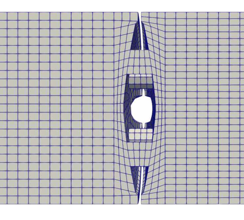
Figure 1: A coarse mesh for a butterfly-valve in use at ATR. In this particular mesh the valve is fully closed.
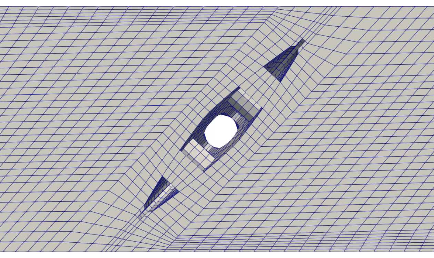
Figure 2: A coarse mesh for a butterfly-valve in use at ATR. In this particular mesh the valve is opened to .
Butterfly-Valve Input
Parameters
The viscosity and density were set to match experimental values for water at the pressure levels measured in earlier experiments. The simulations each begin with the viscosity set at a relatively higher value, but it is ramped-down with each successful timestep. The von-karman constant is a dimensionless constant used in turbulence modeling.
 mu = 0.001 # viscosity [Pa*s]
 rho = 986.737 # density [kg/m^3]
 von_karman_const = 0.41
Mesh
Because of the complex geometries involved, Cubit was used to generate meshes for all angles tested. All meshes used are included with the input file provided. For each angle simulated three meshes (coarse, medium, and fine) were created. Each course mesh had between 50-100 thousand cells, medium meshes between 100-200 thousand cells, and fine meshes over 200 thousand cells. Three levels of refinement were used so that the self convergence rate could be calculated using the method described in Roache (1998).
Boundary Conditions
The inlet-u parameter controls the inlet velocity. Its function value can be changed to match the experimental inlet velocities. To reduce computational resources The entire assembly was split in half in the direction of flow. Since the pipe and valve is symmetric along this axis, a symmetry boundary condition was applied along this surface to approximate simulating the entire assembly. Additionally, the outlet was set as a constant pressure outlet of , and all walls were set as no-slip boundary conditions. The boundary conditions are created by the Physics/NavierStokes/Flow/flow syntax.
Variables
All simulations were done in three dimensions. Because of the turbulent nature of the simulations, a relatively slow initial velocity in the x-direction was chosen. This prevented the simulations from diverging early on. The variables are created by the Physics/NavierStokes/Flow/flow syntax.
[Physics]
  [NavierStokes]
    [Flow]
      [flow]
        compressibility = 'incompressible'

        density = '${rho}'
        dynamic_viscosity = '${mu}'

        # Initial conditions
        initial_velocity = '0.1 0 0'
        initial_pressure = 0

        # Boundary conditions
        inlet_boundaries = 'Inlet'
        momentum_inlet_types = 'fixed-velocity'
        momentum_inlet_functors = '2.051481762 0 0'

        wall_boundaries = 'Walls Valve Symmetry'
        momentum_wall_types = 'noslip noslip symmetry'

        outlet_boundaries = 'Outlet'
        momentum_outlet_types = 'fixed-pressure'
        pressure_functors = '0'

        mass_advection_interpolation = '${advected_interp_method}'
        momentum_advection_interpolation = '${advected_interp_method}'
        velocity_interpolation = '${velocity_interp_method}'
      []
    []
  []
[]
AuxVariables
To implement the mixing-length turbulence model, a mixing_length auxillary variable needs to be included.
The mixing length variable is created by the Physics/NavierStokes/Turbulence/mixing_length syntax.
AuxKernels
This kernel controls the behavior of the mixing-length model. Walls 2 and 4 correspond to the wall of the pipe and the valve, while the delta parameter controls turbulent behavior near these walls.
[Physics]
  [NavierStokes]
    [Turbulence]
      [mixing_length]
        turbulence_handling = 'mixing-length'
        von_karman_const = ${von_karman_const}
        mixing_length_delta = 0.005
      []
    []
  []
[]
Executioner
While these are steady-state simulations, a transient solver must be used in order for the viscosity rampdown to function as intended. This operates by having the viscosity ramp down over time while every other parameter remains unchanged. With each successful timestep, the viscosity approaches the desired value. The simulation terminates once it ramps down all the way to the desired level.
[Executioner]
  type = Transient

  # Time-stepping parameters
  start_time = 0.0
  end_time = 8

  [TimeStepper]
    type = IterationAdaptiveDT
    optimal_iterations = 10
    # Start small, or improve the initial condition
    dt = 0.0125
    timestep_limiting_postprocessor = 'dt_limit'
  []

  # Time integration scheme
  scheme = 'implicit-euler'

  # Solver Parameters
  solve_type = 'NEWTON'
  petsc_options_iname = '-pc_type -pc_factor_shift_type -snes_max_it -l_max_it -max_nl_its'
  petsc_options_value = 'lu       NONZERO                25           50        20        '
  line_search = 'none'
  nl_rel_tol = 1e-6
  nl_abs_tol = 1e-10
  automatic_scaling = true
  scaling_group_variables = 'vel_x vel_y vel_z; pressure'
[]
Viscosity Rampdown
The viscosity rampdown is controlled but two input blocks, the Functions and Materials. The functions block determines how quickly the rampdown occurs while the materials block is what defines the value of mu as show in the listing below. For these simulations, mu was first ramped down to a value of 1e-3 PaS. Once it converged to that point, it was restarted and a new rampdown function was used to quickly bring the viscosity down to 5.4e-4 PaS.
[Functions]
  [rampdown_mu_func]
    type = ParsedFunction
    expression = 'if(t<= 5, mu*(100*exp(-3*t)+1), 0.000463*exp(-3*(t-5))+0.000537)'
    symbol_names = 'mu'
    symbol_values = ${mu}
  []
[]
[FunctorMaterials]
  [mu]
    type = ADGenericFunctorMaterial #defines mu artificially for numerical convergence
    prop_names = 'mu rho' #it converges to the real mu eventually.
    prop_values = 'rampdown_mu_func ${rho}'
  []
  [velocity_vector]
    type = ADGenericVectorFunctorMaterial
    prop_names = vel_vec
    prop_values = 'vel_x vel_y vel_z'
  []
[]
Results
Shown below are velocity and pressure profiles for each angle and for select inlet velocities. These profiles were all taken from the finer mesh simulations. They display expected features such as pressure and velocity peaks in the correct regions.
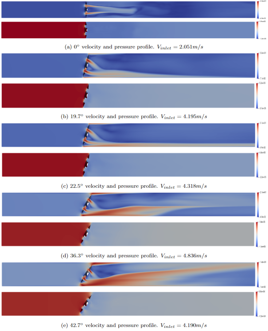
Figure 3: Velocity and pressure profiles for each valve configuration.
Simulations were also performed on the fine mesh using STAR-CCM+ as a point of comparison. The pressure drop, resistance coefficient, and flow coefficient for all configurations (and for STAR-CCM+ simulations) is shown in the figure below. The experimental data was taken from an internal study by Idaho National Laboratory (2008). Also included is a table with the pressure drop error and convergence information for the different levels of mesh refinement. For most of the angles tested, simulations approached experimental value as finer meshes were used, with the only exception being the 22.5 configuration. However for that particular configuration simulation error relative to experimental values was already significantly smaller than other configurations.
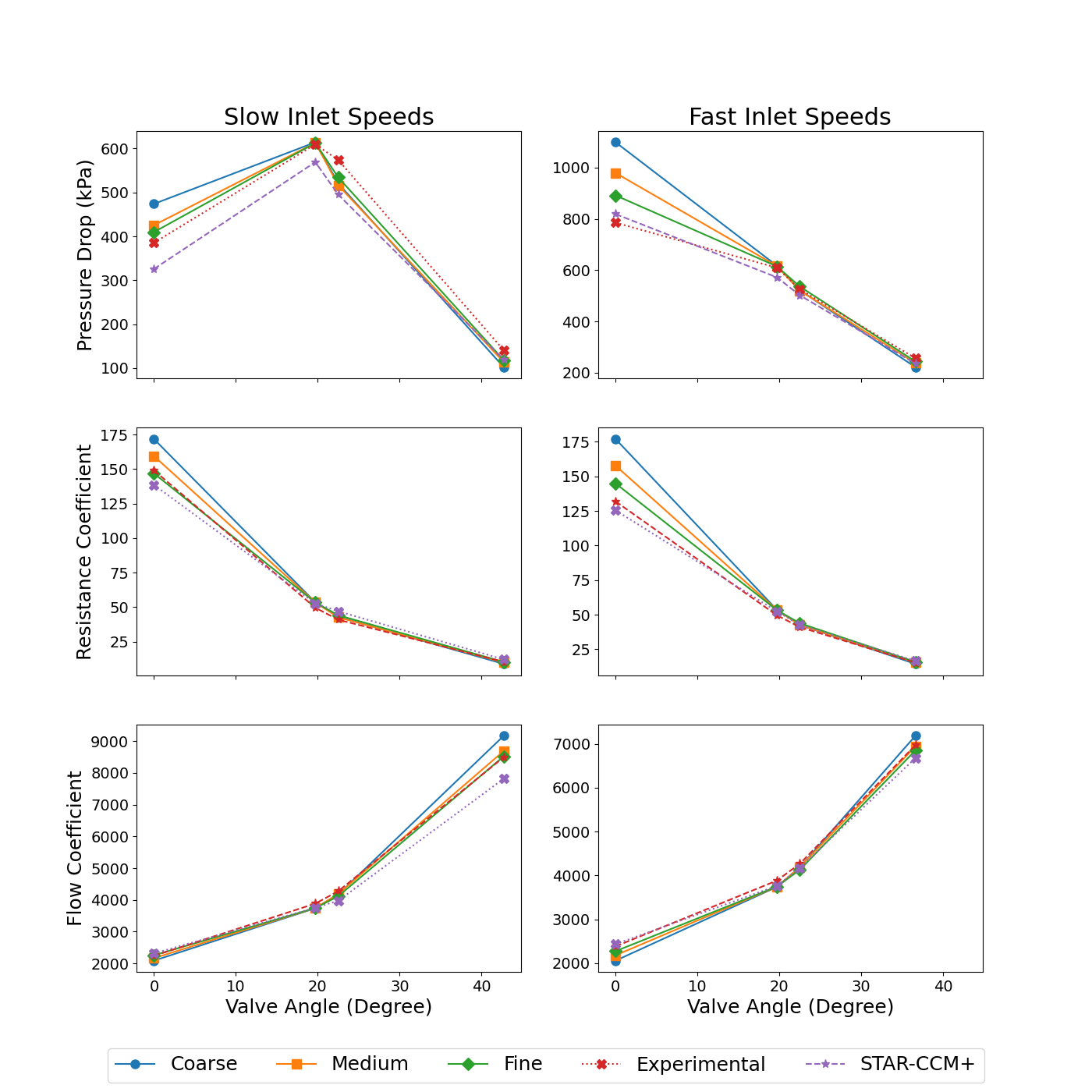
Figure 4: Simulation results for each configuration. The pressure drop, resistance coefficient, and flow coefficient for each mesh and corresponding inlet velocity was compared to experimental data as well as results from STAR-CCM+ using the fine meshes.
| Angle | Flow-rate (m^3/s) | # Cells | % Error to experimental pressure-drop across valve |
|---|---|---|---|
| 0 | 1.26 | 88950 | 23.0 |
| 148770 | 10.4 | ||
| 286216 | 6.33 | ||
| 0 | 1.89 | 88950 | 39.9 |
| 148770 | 24.7 | ||
| 286216 | 13.5 | ||
| 19.7 | 2.57 | 97585 | 0.77 |
| 164566 | 0.55 | ||
| 250125 | 0.50 | ||
| 19.7 | 2.58 | 97585 | 1.28 |
| 164566 | 1.08 | ||
| 250125 | 0.88 | ||
| 22.5 | 2.64 | 88561 | 9.31 |
| 142611 | 10.0 | ||
| 276116 | 6.91 | ||
| 22.5 | 2.66 | 88561 | 0.73 |
| 142611 | 0.95 | ||
| 276116 | 2.03 | ||
| 36.6 | 2.97 | 99184 | 13.7 |
| 174730 | 7.52 | ||
| 254610 | 5.07 | ||
| 42.7 | 2.58 | 92668 | 27.3 |
| 173348 | 19.1 | ||
| 272450 | 15.9 |
References
- P.J. Roache.
Verification and Validation in Computational Science and Engineering.
Hermosa Publishers, Albuquerque, New Mexico, 1998.[BibTeX]
- Idaho National Laboratory.
Update of ATR Primary Coolant System RELAP5 Model.
2008.[BibTeX]
- Idaho National Laboratory.
Water hammer Transient Computational Fluid Dynamics (CFD) Analysis of ATR PCS under Butterfly Valve BF-A-1-14 Failure.
2023.[BibTeX]