Molten Salt Reactor Experiment (MSRE) Lower Plenum CFD Investigation
Contact: Jun Fang, fangj.at.anl.gov
Model link: MSRE Lower Plenum CFD Model
Model Overview
The MSRE was a graphite moderated flowing salt type reactor with a design maximum operating power of 10 MW(th) developed by Oak Ridge National Laboratory (Robertson, 1965). The fuel salt was a mixture of lithium, beryllium, and zirconium fluoride containing uranium or thorium and uranium fluoride. The coolant salt was a mixture of lithium fluoride and beryllium fluoride. The reactor consisted of two flow loops: a primary loop and a secondary loop. The primary loop connected the reactor vessel to a fuel salt centrifugal pump and the shell side of the shell-and-tube heat exchanger. The secondary loop connected the tube-side of the shell-and-tube heat exchanger to a coolant salt centrifugal pump and the tube side of an air-cooled radiator. Two axial blowers supplied cooling air to the radiator. Piping, drain tanks and “freeze valves” made up the remaining components of the heat transport circuits. The heat generated in the core was transferred to the secondary loop through the heat exchanger and ultimately rejected to the atmosphere through the radiator.
Detailed inflow conditions are essential for accurately modeling the three-dimensional reactor physics and thermal fluid behavior within the core region of the MSRE. However, this task is hindered by the lack of comprehensive information about the MSRE's lower plenum. In the MSRE, molten salt flowed from the downcomer into the lower plenum of the reactor core, an area characterized by complex geometries and poorly understood flow patterns. Figure 1 illustrates the lower core region, comprising a lower vessel head with anti-swirl vanes and a drain line attachment. When the salt entered the lower plenum from the downcomer annulus, it retained a tangential component to its flow. Without correction, this would have caused a significant pressure gradient in the lower head, leading to an uneven distribution of flow throughout the core. To address this issue, anti-swirl vanes were introduced to the lower vessel head. These vanes consisted of 48 plates, starting approximately 2 inches up in the core wall cooling annulus and extending radially into the lower head for about 38% of the radial distance to the core centerline. More detailed geometric information can be found in the ORNL report by Kedl (1970).
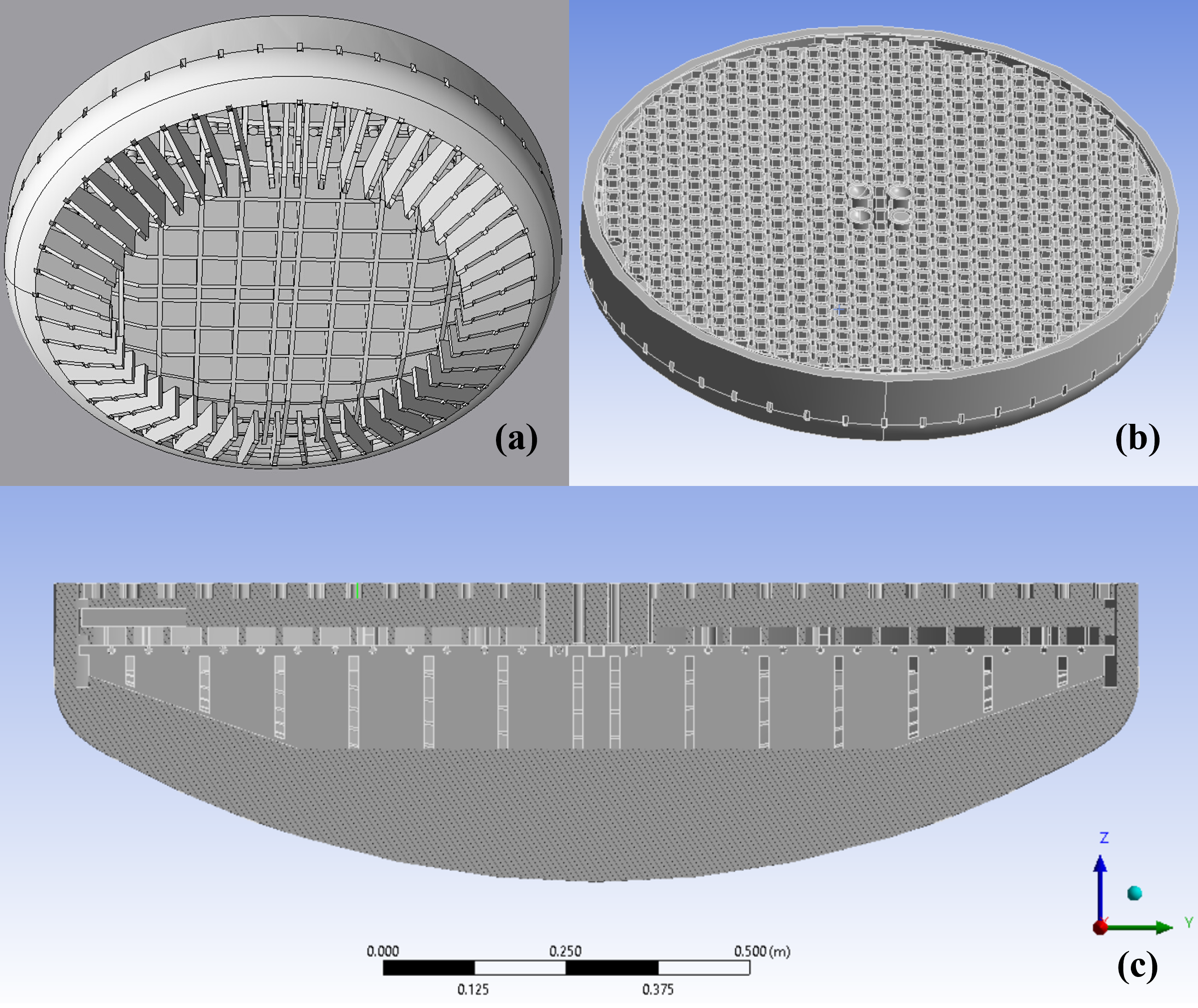
Figure 1: Geometric model of MSRE lower plenum: (a) the bottom view with MSRE lower head surface hidden to show internal structures such as anti-swirl fans, support grid, etc.; (b) the top view to show the annulus inlet from downcomer and outlet channels into the MSRE core region; (c) a slice view through MSRE lower plenum.
The discretization and numerical models used by the CFD flow solver Nek5000/RS can be found on MSFR CFD documentation webpage.
CFD Case Setups
Model creation and meshing
A geometric model of the MSRE full core was obtained through the collaboration with Copenhagen Atomics (Stubsgaard, 2023). As shown in Figure 1, the lower plenum portion is taken out from the full core model and prepared for the meshing process. A computational mesh consisting of tetrahedral and wedge cells is first created using 3rd party meshing software, ANSYS Mesh. Due to the presence of numerous small features within the original CAD model, several adjustments were made to facilitate practical mesh generation. This involved removing minor structures, such as the narrow gaps between mounting rods and the horizontal plates to which the rods are connected. Since the nekRS spectral element code requires a pure hexahedral mesh for calculations, an additional step was necessary to convert the initial mesh, created in Exodus format by ANSYS Mesh, into the nekRS-supported re2 format.
To maintain the accuracy of geometric features, the latest quadratic tet-to-hex converter was employed, improving upon the previous linear tet-to-hex converter and enhancing the resolution of surface curvature, particularly along circular boundaries. It's important to note that, due to technical challenges associated with implementing a boundary layer mesh, the computational grid shown in Figure 2 does not feature a more refined mesh near the wall surfaces. This was a deliberate compromise to maintain reasonable mesh quality and cell count. While this choice may impact simulation accuracy with respect to capturing near-wall flow physics, it is deemed justifiable, given that the primary objective is to analyze velocity distribution in the lower plenum outlet channels. Additionally, it's expected that the velocity gradient will be relatively modest on most of the lower plenum walls. The resulting mesh comprises 23.6 million cells, and with a polynomial order of 3, the total number of unique grid points amounts to approximately 664 million in actual nekRS calculations.
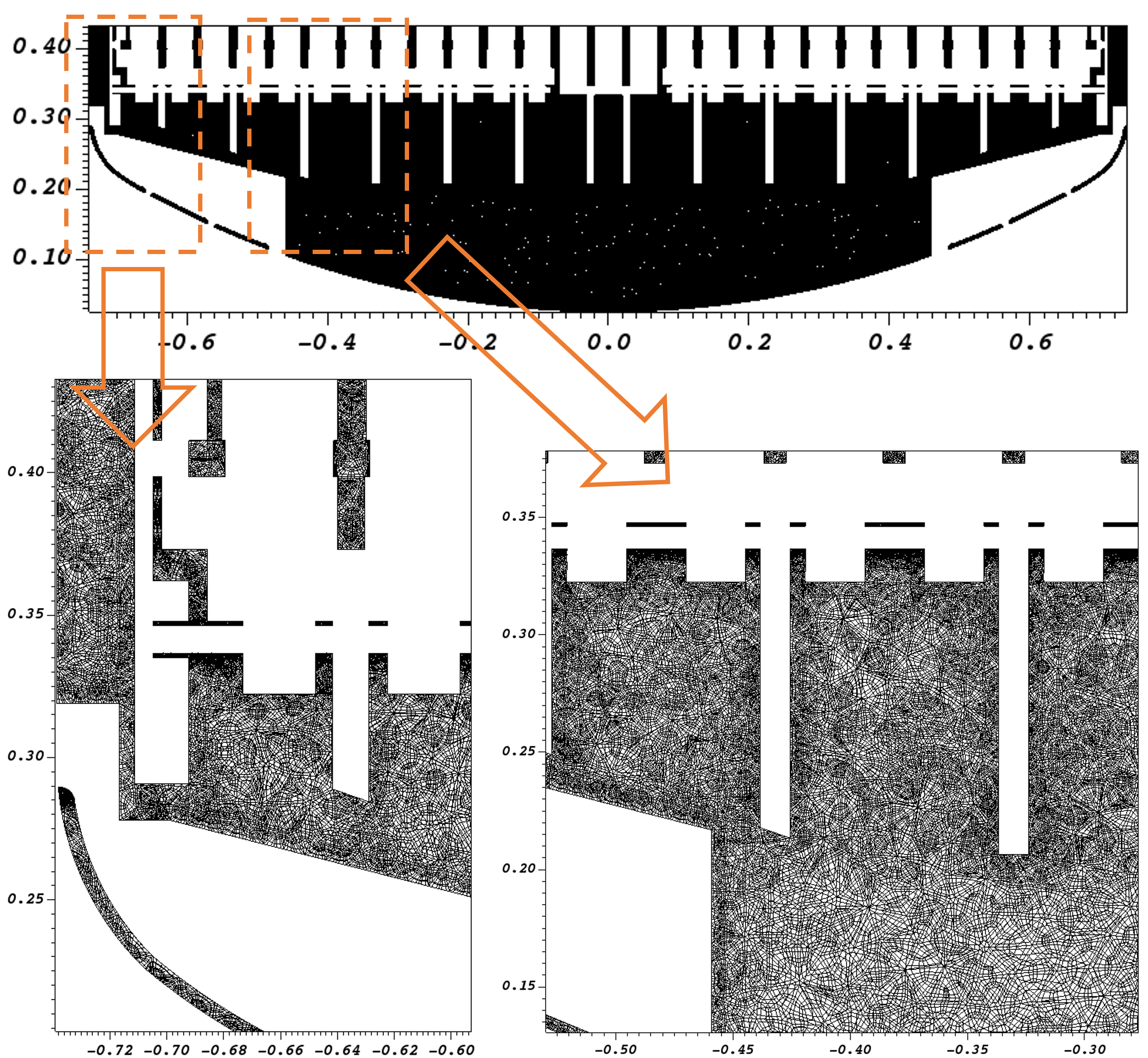
Figure 2: Overview and detailed views of the computational mesh for MSRE lower plenum.
For the MSRE lower plenum CFD simulations, the choice of salt composition is Salt C (LiF-BeF4-ZrF4-UF4) as reported by Beall et al. (1964). Table 1 provides the relevant material properties for this fuel salt. With an anticipated volume flow rate of 1200 gallons per minute (gpm) for the MSRE system, we can expect the average velocity of the salt as it enters the lower plenum from the annulus downcomer to be approximately 0.6553 m/s. This results in an estimated Reynolds number of approximately 4321.57, indicating that the flow is in a transitional state between laminar and turbulent regimes. Given the larger flow areas in the lower plenum, the local Reynolds number may be even lower within that region. Consequently, it has been decided to employ a LES approach instead of utilizing RANS modeling techniques.
Table 1: MSRE fuel salt properties and lower plenum flow conditions.
| Unit | LiF-BeF-ZrF-UF | ||
|---|---|---|---|
| Salt density | |||
| Salt dynamic viscosity | |||
| Salt kinematic viscosity | |||
| Downcomer annulus thickness | |||
| Mean salt velocity | |||
| Reynolds number at downcomer |
Diving into nekRS case files
Readers can access the nekRS case files and the corresponding mesh files in the VTB repository via GitHub Large File Storage (LFS). The mesh data is contained in two files: msre.re2 (which includes grid coordinates and sideset ids) and msre.co2 (containing mesh cell connectivity information). Regarding the nekRS case files, there are four basic files:
msre.udf serves as the primary nekRS kernel file and encompasses algorithms executed on the hosts. It's responsible for configuring CFD models when needed, collecting time-averaged statistics, and determining the frequency of calls to userchk, which is defined in the usr file.
msre.oudf is a supplementary file housing kernel functions for devices and also plays a role in specifying boundary conditions.
msre.usr is a legacy file inherited from Nek5000 and can be utilized to specify initial conditions and define post-processing capabilities.
msre.par is employed to input simulation parameters, including material properties, time step size, and Reynolds number, etc.
There are also supportive scripts in the case folder. linearize_bad_elements.f and BAD_ELEMENTS are used to fix the mesh cells that potentially have negative Jacobian values from the quadratic tet-to-hex conversion.
Now let's first explore the key case file msre.usr. The sideset ids contained in the mesh file are translated into nekRS boundary condition information in usrdat2 block. It is preferred to conduct nekRS CFD simulations in a non-dimensional manner. Thus, we also did the geometry rescaling here such that the reference length, which is the donwcomer annulus thickness, is 1.0.
      subroutine usrdat2()  ! This routine to modify mesh coordinates
      include 'SIZE'
      include 'TOTAL'

      integer iel, ifc, id_face, ntot
      integer i, e, f
      real ti

      do iel=1,nelv
      do ifc=1,2*ndim
        id_face = bc(5,ifc,iel,1)
        boundaryID(ifc,iel)  = 0
        if (id_face.eq.2) then
           cbc(ifc,iel,1) = 'v  '
           boundaryID(ifc,iel)  = 1
        elseif (id_face.eq.3) then
           cbc(ifc,iel,1) = 'O  '
           boundaryID(ifc,iel)  = 2
        elseif (id_face.eq.4) then
           cbc(ifc,iel,1) = 'W  '
           boundaryID(ifc,iel)  = 3
        else
           cbc(ifc,iel,1) = 'E  '
           boundaryID(ifc,iel)  = 0
        endif
      enddo
      enddo

C Rescale the geometry so that the downcomer annulus thickness is 1.0
      ntot = nelt*lx1*ly1*lz1
      ti = 1.0/0.0254
      do i=1,ntot
        xm1(i,1,1,1)=xm1(i,1,1,1)*ti
        ym1(i,1,1,1)=ym1(i,1,1,1)*ti
        zm1(i,1,1,1)=zm1(i,1,1,1)*ti
      enddo

      return
      end
c-----------------------------------------------------------------------
The fixes to the possible negative Jacobian errors in mesh file is called in usrdat
      subroutine usrdat   ! This routine to modify element vertices
      include 'SIZE'      ! _before_ mesh is generated, which
      include 'TOTAL'     ! guarantees GLL mapping of mesh.

      integer n_correction
      real minJacobian

      n_correction = 2
      call linearize_bad_elements(n_correction)  ! 2 (iterations for correction) should be enough, if not, set to 3

      minScaleJacobian = 1e-3
      call linearize_low_jacobian_elements(n_correction,
     & minScaleJacobian) ! linearize element that with lower jacobian than minJacobian

      return
      end
c-----------------------------------------------------------------------
The intended LES simulations can be readily configured in the simulation input file msre.par using the code snippet below. For more information on Nek5000/nekRS LES filtering, interested readers are referred to Nek5000 turtorial.
regularization = hpfrt + nModes=1 + scalingCoeff=10
subCyclingSteps = 2
To maintain a balance between numerical stability and simulation efficiency, a variable time step sizing is implemented. The simulation utilizes an Operator-Integration-Factor Splitting (OIFS) scheme to mitigate the CFL restrictions arising from the small-size mesh cells resulting that are created by unstructured meshing and tet-to-hex conversion. A minimum time step of is specified with the target CFL number at around 3.0.
dt = targetCFL=3 + initial=2e-5
A constant inflow velocity is given to the downcomer annulus surface.
void velocityDirichletConditions(bcData *bc)
{
  bc->u = 0.0;
  bc->v = 0.0;
  bc->w =-1.0;
}
Time averaged statitics is collected using the following lines in msre.udf
  5 #include "plugins/tavg.hpp"

 19   tavg::setup(nrs);

 24   tavg::run(time);
 25
 26   if (nrs->isOutputStep) {
 27     tavg::outfld();
 28   }
Results
Figure 3 provides an instantaneous snapshot of the velocity distribution in the lower plenum. The flow of molten salt into the lower plenum occurs through an annulus downcomer in the peripheral region. Upon entry, the salt comes into contact with anti-swirl fans that are installed on the MSRE lower head. These 48 fans are designed to effectively eliminate most of the circumferential velocity components that develop in the downcomer. It's important to note that in the bulk region of the lower plenum, the velocity magnitude is quite low. This suggests that using a Reynolds-Averaged Navier-Stokes (RANS) model may not be necessary for modeling this flow behavior. Above the anti-swirl fans, there is the main support grid, which bears the weight of the MSRE core. Some flow recirculations are observed as the salt flows past the bottom tips of the support grid. Moving further above the main support grid, there are two layers of horizontal plates that serve to secure the graphite stringers in place. These plates often have small gaps, which further restrict the lateral movement of the molten salt. Due to the presence of anti-swirl fans and other structures in the lower plenum, the circumferential fluid motion is completely eliminated by the time the salt reaches the outlet channels. Regarding the vertical velocity component, it's noteworthy that the central region experiences the highest upward flow.
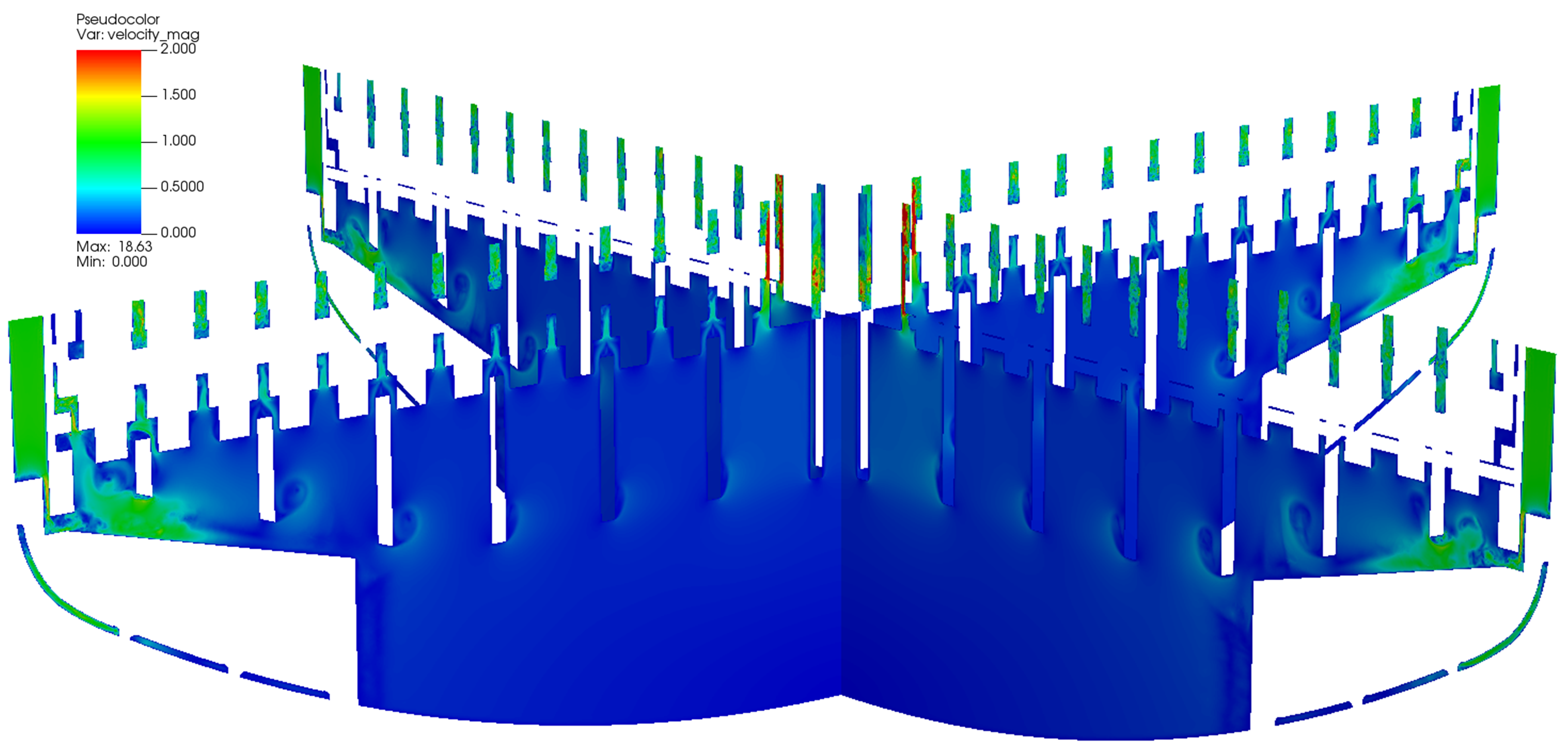
Figure 3: Instantaneous velocity distribution in MSRE lower plenum.
For a more detailed insight into the radial distribution of upward flow from the MSRE lower plenum, Figure 4 provides a clearer perspective. As the molten salt enters the lower plenum through the peripheral annulus inlet, it carries a higher magnitude of velocity. Figure 4 also offers a distinct view of the main support grid. In this context, a high-velocity area is discernible in the central region, while a relatively lower-velocity area is evident in the middle section. To provide a more quantitative description of this radial distribution of upward flow as the salt reaches the outlet channels, additional post-processing has been performed on the time averaged data.
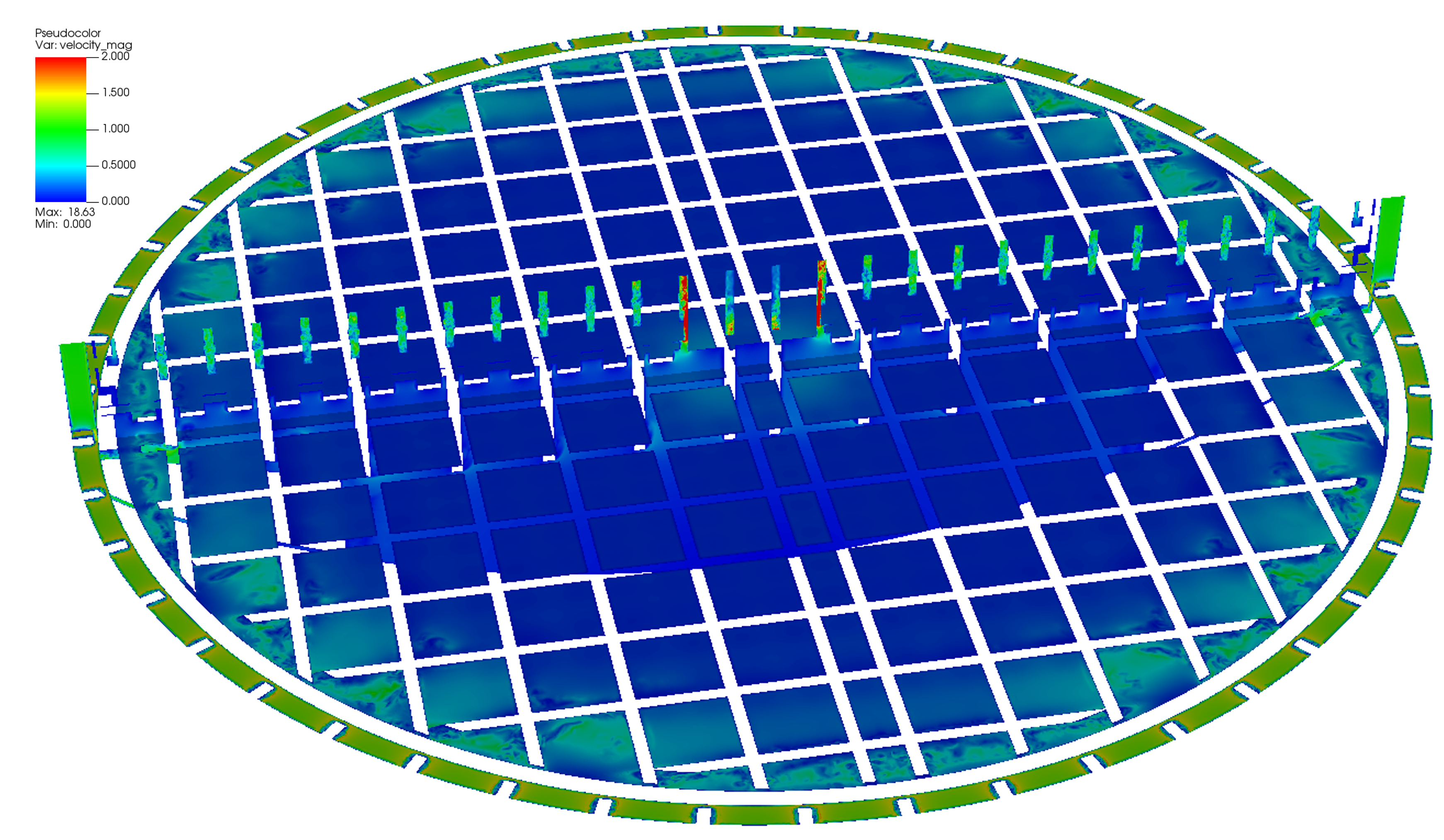
Figure 4: Radial distribution of instantaneous velocity in MSRE lower plenum.
Additional nekRS simulations were conducted to gather time-averaged flow data within the MSRE lower plenum. The complete MSRE core possesses a diameter of 28 inches, and to organize the flow channels effectively, they have been categorized into five groups based on their radial positions: 0-5, 5-10, 10-15, 15-20, and 20-28 inches, as depicted in Figure 5. To calculate group-averaged outlet velocities for each of these groups, a post-processing algorithm for surface averaging was developed within nekRS. These velocities are subsequently normalized using the mean vertical velocity across all outlet channels. The resulting quantitative outlet channel profiles are presented in Figure 6. Notably, the central group, referred to as Group 1, exhibits the highest averaged velocity, surpassing the mean outlet velocity by 58%. In contrast, the middle section, comprising groups 2, 3, and 4, exhibits velocities approximately 10% lower than the mean value. The averaged velocity then increases again in the outermost peripheral group. This velocity profile data plays a crucial role in defining more accurate inlet boundary conditions for subsequent multiphysics simulations within the MSRE core region.
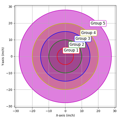
Figure 5: Grouping of the outlet channels based on radial locations.
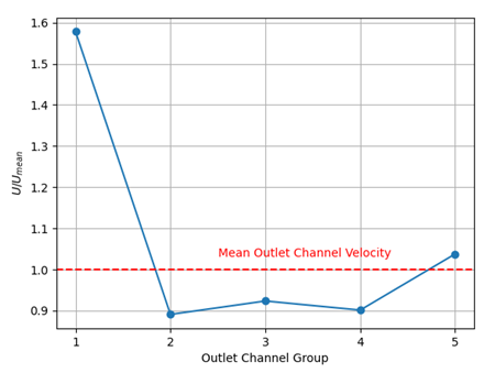
Figure 6: Group averaged velocities into the MSRE core region.
References
- S E Beall, P N Haubenreich, R B Lindauer, and J R Tallackson.
MSRE Design and Operations Report. Part V. Reactor Safety Analysis Report.
Technical Report ORNL-TM-732, Oak Ridge National Laboratory, Oak Ridge, TN, 1964.[BibTeX]
- R. J. Kedl.
Fluid Dynamic Studies of the Molten Salt Reactor Experiment (MSRE) Core.
Technical Report ORNL-TM-3229, Oak Ridge National Laboratory, Oak Ridge, TN, 1970.[BibTeX]
- R C Robertson.
MSRE design and operations report. Part I. Description of reactor design.
Technical Report ORNL-TM-728, Oak Ridge National Laboratory, Oak Ridge, TN, 1965.[BibTeX]
- Aslak Stubsgaard.
OPENMSR.
2023.
URL: https://github.com/openmsr/msre (visited on 2023-09-07).[BibTeX]