Cardinal Model of Thermal Striping Phenomenon in MSR Piping System
Contact: Jun Fang, fangj.at.anl.gov
Model link: Thermal Striping Cardinal Model
Model Overview
This tutorial documents a demonstration study recently conducted to showcase the advanced NEAMS multiphysics capabilities for modeling the thermal striping phenomenon commonly observed in reactor pipeline systems. The study employed the state-of-the-art multiphysics simulation framework, Cardinal. A T-junction geometry was selected as the computational domain, featuring two inlets with different temperatures and one outlet. The interaction between the hot and cold inflows is expected to cause strong mixing within the T-junction, leading to temperature oscillations on the pipe walls. The multiphysics coupling involves using NekRS to perform high-fidelity conjugate heat transfer (CHT) calculations, predicting temperature distributions in both the solid (pipe wall) and fluid regions. These solid temperatures are then passed to the MOOSE Solid Mechanics Module for thermal stress analysis. In this document, we provide a step-by-step guide to setting up the related nekRS and Cardinal cases, along with a brief discussion of the results obtained.
nekRS Case Setups
The T-junction model is illustrated in Figure 1, where strong mixing is anticipated as the inflows from the horizontal and vertical inlets converge at the joint. We selected molten salt LiF-BeF2 as the fluid due to its critical role as a coolant salt in the Molten Salt Reactor Experiment (MSRE) (Beall et al., 1964). The horizontal inflow temperature is 900 K, while the vertical inflow temperature is 1000 K, with both inlets having a fixed velocity of 20 cm/s. The fluid properties, including density, viscosity, and thermal conductivity, are assumed to be constant, and their values are listed in Table 1 for the conjugate heat transfer (CHT) calculations. The pipe shell is assumed to consist of Hastelloy N alloy, with its thermo-physical properties detailed in Table 2 (Fang et al., 2020).
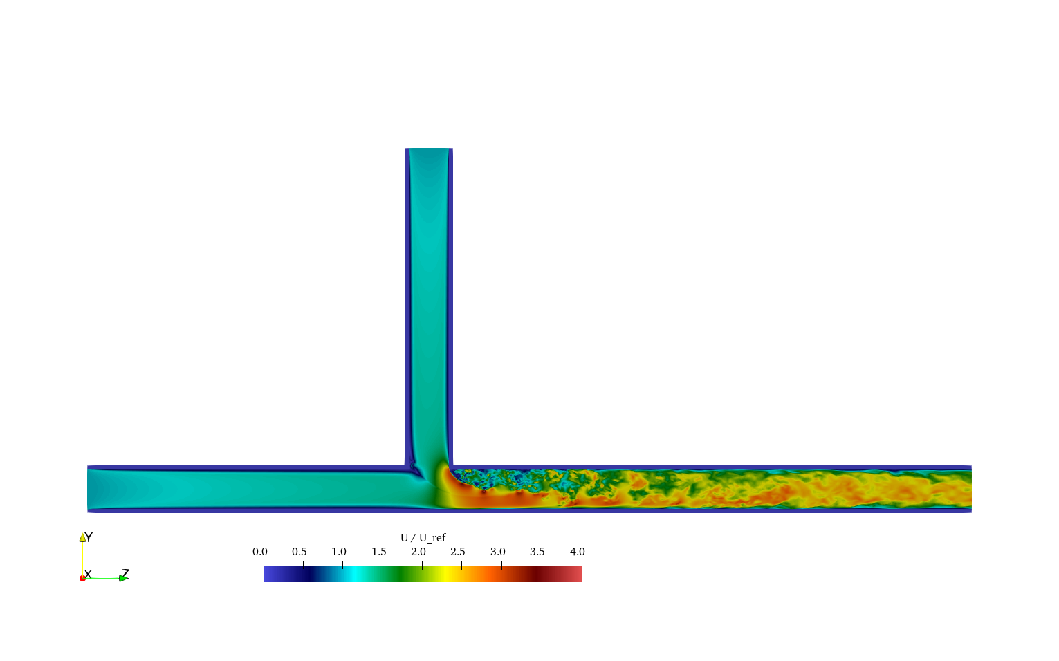
Figure 1: Velocity distribution inside the T-junction pipes.
Table 1: Fluid properties of the molten salt.
| Parameters | Value | Unit |
|---|---|---|
| Density | 1682.32 | |
| Dynamic viscosity | 6.04E-03 | |
| Thermal conductivity | 1.1 | |
| Specific heat capacity | 2390 | |
| Inlet velocity | 0.2 | |
| Reynolds number | 2785.12 | |
| Prandtl number | 13.12 | |
| Peclet number | 36552.23 |
Table 2: Solid properties of Hastelloy N alloy.
| Parameters | Value | Unit |
|---|---|---|
| Density | 8860 | |
| Thermal conductivity | 23.6 | |
| Specific heat capacity | 578 | |
| Young's modulus | 171 | |
| Poisson's ratio | 0.31 | |
| Thermal expansion coefficient | 1.38E-05 |
The discretization of the CFD model results in 365,568 mesh elements in the fluid region and 129,024 elements in the solid region. The fluid and solid regions share a conformal mesh at the coupling interface. Given the moderate Reynolds number of 2785.12 expected in the T-junction, the Large Eddy Simulation (LES) approach is employed in the NekRS spectral element simulations (Fischer et al., 2022). With a polynomial order of 5, the total degrees of freedom are approximately 62 million. The CFD results of the temperature distributions are presented in Figure 2. Due to the hot inflow, the shell of the vertical pipe heats up, particularly in the region near the vertical entrance. In the horizontal section, the cold molten salt dominates from the horizontal entrance to the joint, with strong temperature mixing observed downstream of the joint. The T-junction configuration causes the upper side of the pipe shell to experience consistently higher temperatures than the bottom side.
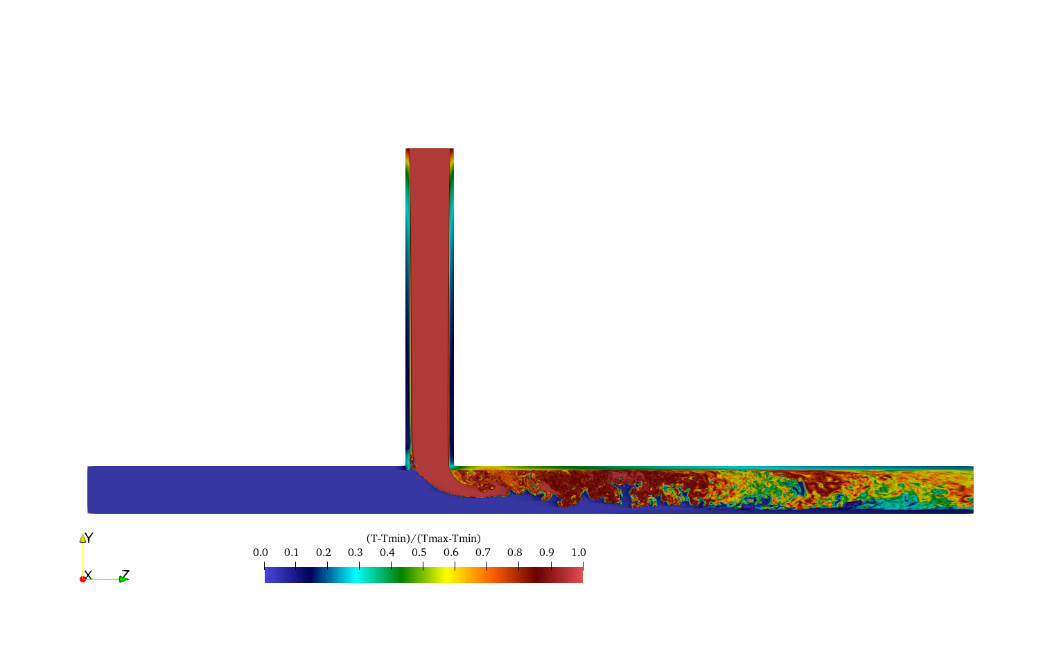
Figure 2: Velocity distribution inside the T-junction pipes.
nekRS case files
Readers can access the nekRS case files and the corresponding mesh files in the VTB repository via GitHub Large File Storage (LFS). The mesh data is contained in two files: tjunc.re2 (which includes grid coordinates and sideset ids) and tjunc.co2 (containing mesh cell connectivity information). Regarding the nekRS case files, there are four basic files:
tjunc.udfserves as the primary nekRS kernel file and encompasses algorithms executed on the hosts (i.e., CPUs). It's responsible for configuring CFD models when needed, collecting time-averaged statistics, and determining the frequency of calls touserchk, which is defined in the usr file.tjunc.oudfis a supplementary file housing kernel functions for devices (i.e., GPUs) and also plays an important role in specifying boundary conditions.tjunc.usris a legacy file inherited from Nek5000 and can be utilized to set up boundary condition tag, specify initial conditions, and define post-processing capabilities.tjunc.paris employed to input simulation parameters, including material properties, time step size, and Reynolds number, etc.
Now let's first explore the case file tjunc.usr. The sideset ids contained in the mesh file are translated into nekRS boundary condition tags in usrdat2 block. There are two inlets (boundary 1 - vertical, and boundary 2 - horizontal) and one outlet (boundary 3) for the fluid region, while the solid region, namely, the T-junction wall has two surfaces, an inner surface (no boundary ID required) in contact with the flowing molten salt and an outer surface (boundary 4), which is assumed to be adiabatic in this study.
      subroutine usrdat2
      include 'SIZE'
      include 'TOTAL'

C Set up boundary conditions
      do iel=1,nelt
         ieg = lglel(iel)
      do ifc=1,2*ndim
         boundaryID(ifc,iel)  = 0
         boundaryIDt(ifc,iel) = 0
         if (bc(5,ifc,iel,1).eq.2) then      !vertical inlet
            cbc(ifc,iel,1) = 'v  '
            cbc(ifc,iel,2) = 't  '
            boundaryID(ifc,iel)  = 1
            boundaryIDt(ifc,iel) = 1
         elseif (bc(5,ifc,iel,1).eq.5) then  !horizontal inlet
            cbc(ifc,iel,1) = 'v  '
            cbc(ifc,iel,2) = 't  '
            boundaryID(ifc,iel)  = 2
            boundaryIDt(ifc,iel) = 2
         elseif (bc(5,ifc,iel,1).eq.3) then  !outlet
            cbc(ifc,iel,1) = 'O  '
            cbc(ifc,iel,2) = 'I  '
            boundaryID(ifc,iel)  = 3
            boundaryIDt(ifc,iel) = 3
         elseif (bc(5,ifc,iel,1).eq.4) then  !walls
            cbc(ifc,iel,1) = 'W  '
            boundaryID(ifc,iel)  = 4         !temp BC on walls is not needed for CHT
         endif

         if (ieg.gt.nelgv) then              !solid
         if (bc(5,ifc,iel,2).eq.2) then
            cbc(ifc,iel,2) = 'I  '
            boundaryIDt(ifc,iel) = 4
         endif
         endif
      enddo
      enddo

      return
      end
c-----------------------------------------------------------------------
Next, let's examine the case file tjunc.udf. The userq() function is used to specify the heat source term for temperature calculations or any source terms for the transport equations of passive scalars. In this study, no volumetric heat source is considered for either the fluid or salt regions, so the corresponding source terms are set to zero.
void userq(nrs_t *nrs, double time, occa::memory o_S, occa::memory o_FS)
{
  cds_t *cds = nrs->cds;
  mesh_t *mesh = cds->mesh[0];
  const dfloat qvolFluid = 0.0;
  const dfloat qvolSolid = 0.0;
  cFill(mesh->Nelements, qvolFluid, qvolSolid, mesh->o_elementInfo, o_FS);
}
The uservp() function defines the material properties for both the fluid and solid regions in conjugate heat transfer simulations. These properties are non-dimensionalized according to nekRS simulation conventions. Consequently, a dimensional conversion is required to transform the raw nekRS results back into dimensional quantities. This conversion is handled automatically by Cardinal, with users simply needing to provide the reference quantities in the input file nek.i, which will be discussed in the next section.
void uservp(nrs_t *nrs,
            double time,
            occa::memory o_U,
            occa::memory o_S,
            occa::memory o_UProp,
            occa::memory o_SProp)
{
  cds_t *cds = nrs->cds;

  if (updateProperties) {
    if (platform->comm.mpiRank == 0) {
      std::cout << "updating properties"
                << "\n";
    }
    const dfloat rho = 1.0;
    const dfloat mue = 1 / 2785.12;
    const dfloat rhoCpFluid = rho * 1.0;
    const dfloat conFluid = mue * (1 / 13.12);
    const dfloat rhoCpSolid = rhoCpFluid * 1.27;
    const dfloat conSolid = conFluid * 21.45;

    // velocity
    const occa::memory o_mue = o_UProp.slice(0 * nrs->fieldOffset);
    const occa::memory o_rho = o_UProp.slice(1 * nrs->fieldOffset);
    cFill(nrs->meshV->Nelements, mue, 0, nrs->meshV->o_elementInfo, o_mue);
    cFill(nrs->meshV->Nelements, rho, 0, nrs->meshV->o_elementInfo, o_rho);
    // temperature
    const occa::memory o_con = o_SProp.slice(0 * cds->fieldOffset[0]);
    const occa::memory o_rhoCp = o_SProp.slice(1 * cds->fieldOffset[0]);
    cFill(cds->mesh[0]->Nelements, conFluid, conSolid, cds->mesh[0]->o_elementInfo, o_con);
    cFill(cds->mesh[0]->Nelements, rhoCpFluid, rhoCpSolid, cds->mesh[0]->o_elementInfo, o_rhoCp);
    updateProperties = 0;
  }
}
Given the moderate Reynolds number expected in the T-junction pipe, a LES simulation approach is adopted which can be readily configured in the simulation input file tjunc.par using the code snippet below. For more information on Nek5000/nekRS LES filtering, interested readers are referred to Nek5000 tutorial.
regularization = hpfrt + nModes = 1 + scalingCoeff = 20
As part of the boundary condition configuration, a set of boundary tags is specified in the input parameter file to match the definitions provided in the usrdat2 subroutine within the tjunc.usr file.
[VELOCITY]
boundaryTypeMap = v, v, O, W
residualTol = 1e-08

[TEMPERATURE]
boundaryTypeMap = t, t, I, I
residualTol = 1e-08
The specific boundary condition values, such as inflow velocities and temperatures, are provided in the case file tjunc.oudf. In this setup, the inflow velocity magnitude is set to 1.0 for both the horizontal and vertical inlets, while a non-dimensional temperature of 1.0 is assigned to the vertical inlet.
void velocityDirichletConditions(bcData *bc)
{
  bc->u = 0.0;
  bc->v = 0.0;
  bc->w = 0.0;
  if(bc->id==1) { //vertical inlet
     bc->v =-1.0;
    }
  if(bc->id==2) { //horizontal inlet
     bc->w = 1.0;
    }
}

void scalarDirichletConditions(bcData *bc)
{
  bc->s = 0.0;
  if(bc->id==1) { //vertical inlet
     bc->s = 1.0;
    }
}
Cardinal Case Setups
The demonstration model utilizes nekRS to perform conjugate heat transfer simulations and transfer the temperature solution in the solid region (specifically, the T-junction pipe wall) from nekRS to the MOOSE Solid Mechanics Module for thermal stress analysis. This multiphysics coupling approach involves two input files: cardinal.i and nek.i. In this setup, the MOOSE Solid Mechanics model defined in cardinal.i acts as the parent application, while the nekRS CFD model operates as the sub-application. Let's first examine the input file cardinal.i. A solid region mesh has to be provided in Exodus format, with the mesh cells configured as Hex8 elements. In this case, the CFD meshing software ANSYS ICEM was used to generate the mesh.
[Mesh]
  type = FileMesh
  file = solid_hex8.exo
[]A default configuration is used for the MOOSE Solid Mechanics calculations.
[Physics]
  [SolidMechanics]
    [QuasiStatic]
      [all]
        strain = SMALL
        incremental = true
        add_variables = true
        eigenstrain_names = eigenstrain
        generate_output = 'strain_xx strain_yy strain_zz stress_xx stress_yy stress_zz'
      []
    []
  []
[]For the boundary conditions in the Solid Mechanics simulation, the inner surface of the pipe is assumed to remain fixed, while the outer surface is free to move and deform.
[BCs]
  [no_x]
    type = DirichletBC
    variable = disp_x
    boundary = '3'
    value = 0.0
  []
  [no_y]
    type = DirichletBC
    variable = disp_y
    boundary = '3'
    value = 0.0
  []
  [no_z]
    type = DirichletBC
    variable = disp_z
    boundary = '3'
    value = 0.0
  []
[]The solid material properties are specified in the block [Materials], and the specific values can be found in Table 2
[Materials]
  [elasticity_tensor]
    type = ComputeIsotropicElasticityTensor
    youngs_modulus = 1.71e11
    poissons_ratio = 0.31
  []
  [small_stress]
    type = ComputeFiniteStrainElasticStress
  []
  [thermal_expansion_strain]
    type = ComputeThermalExpansionEigenstrain
    stress_free_temperature = 900
    thermal_expansion_coeff = 1.38e-5
    temperature = temperature
    eigenstrain_name = eigenstrain
  []
[]The [MultiApps] block controls the coupling hierarchy, while the volume mapping of the temperature solution from the CFD mesh to the MOOSE mesh is configured in the [Transfers] block.
[MultiApps]
  [nek]
    type = TransientMultiApp
    app_type = CardinalApp
    input_files = 'nek.i'
    sub_cycling = true
    execute_on = timestep_end
  []
[][Transfers]
[nek_bulk_temp_to_moose]
type = MultiAppGeneralFieldNearestLocationTransfer
source_variable = temp
variable = temperature
from_multi_app = nek
# Reduces transfers efficiency for now, can be removed once transferred fields are checked
bbox_factor = 10
[]
[]The nek.i input file orchestrates the CFD simulation performed by nekRS. Its content is quite minimal, with the key settings being the reference values used for converting raw nekRS results into physical quantities of interest in dimensional units. We also specify that we will read the NekRS temperature into a variable named temp (which was referenced earlier in the cardinal.i [Transfers] block).
[Problem]
  type = NekRSProblem
  casename = 'tjunc'

  [Dimensionalize]
    U = 0.2
    T = 900
    dT = 100
    rho = 1682.32
    Cp = 2390
  []

  [FieldTransfers]
    [temp]
      type = NekFieldVariable
      direction = from_nek
      field = temperature
    []
  []
[]Preliminary Results
Leveraging the high-fidelity temperature solutions predicted by NekRS, Cardinal maps these solutions onto an intermediate MOOSE mesh. These temperature solutions can then be utilized by any MOOSE application, such as the MOOSE Solid Mechanics Module, which uses the temperature information to perform subsequent thermal stress analysis. The temperature and thermal stresses experienced by the T-junction pipe shell are detailed in Figure 3. The thermal stress profiles correspond closely to the temperature distribution, with significant variations in thermal stresses observed at the vertical entrance region and the upper side of the horizontal pipe after the joint. Overall, this study demonstrates that Cardinal is well-suited for modeling the thermal striping phenomenon.
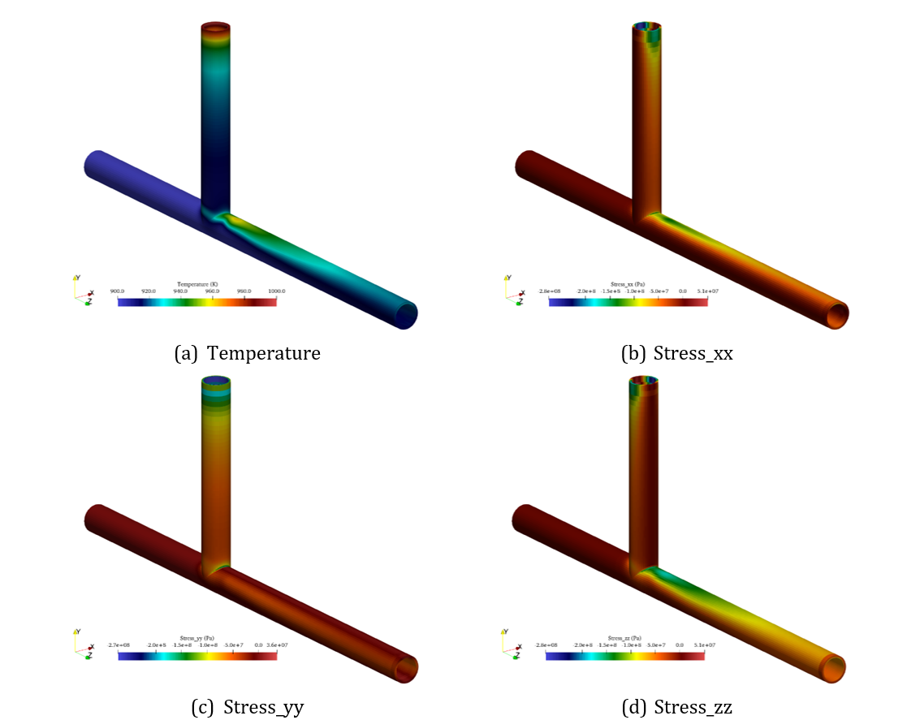
Figure 3: Pipe shell temperature and thermal stress components from MOOSE Solid Mechanics.
Run Command
This particular Cardinal case was executed using 8 GPUs on a local HPC cluster with the Slurm job scheduler. A job submission script, gpuCardinal, was created to submit the simulation to the HPC queue. The script's usage is straightforward, requiring the following input arguments: %job_name% %number_of_gpus% %runtime_hours% %runtime_minutes%.
./gpuCardinal cardinal 8 02 00
The content of the gpuCardinal script is provided below, and users can modify it for use on other HPC platforms as needed.
#!/usr/bin/env bash

[ $# -ne 4 ] && echo "gpuCardinal requires 4 arguments: %job_name% %number_of_gpus% %runtime_hours% %runtime_minutes%" && exit 0;

# the paths have to be updated for specific cardinal build
PATH+=:/beegfs/scratch/fangj/Cardinal/cardinal
export NEKRS_HOME=/beegfs/scratch/fangj/Cardinal/cardinal/install

# the compilers and modules have to be updated for specific HPC platforms
export CC=mpicc
export CXX=mpicxx
export FC=mpif90
module load openmpi/4.1.5/gcc/9.3.1-cuda cmake/cmake-3.24 anaconda3/anaconda3

ngpus=$2
[ $ngpus -gt 16 ] && echo "only 16 gpus available" && exit 0;

if [[ $ngpus -gt 8 ]]; then
  nnodes=2
  res=$(( $ngpus % 2 ))
  [ $res -ne 0 ] && ngpus=$(($ngpus+1))
  ntpn=$(( $ngpus / 2 ))
else
  nnodes=1
  ntpn=$ngpus
fi

cmd="cardinal-opt -i $1.i"

printf -v tme "%0.2d:%0.2d" $3 $4
echo "submitting Cardinal job \"$cmd\" on $(($nnodes * $ntpn)) gpus for $tme"

echo   "#!/bin/bash"                              >  $1.batch
echo   "#SBATCH --nodes=$nnodes"                  >> $1.batch
echo   "#SBATCH --ntasks-per-node=$ntpn"          >> $1.batch
echo   "#SBATCH --gres=gpu:$ntpn"                 >> $1.batch
echo   "#SBATCH --time="$tme":00"                 >> $1.batch
echo   "#SBATCH -p gpu"                           >> $1.batch
echo   "#SBATCH -o $1.%A.log"                     >> $1.batch
echo   "source $envfile"                          >> $1.batch
echo   "export PSM2_CUDA=1"                       >> $1.batch
echo   "export MPICH_GPU_SUPPORT_ENABLED=1"       >> $1.batch
echo   rm -f  logfile                             >> $1.batch
echo   touch $1.\$SLURM_JOBID.log                 >> $1.batch
echo   ln -s $1.\$SLURM_JOBID.log logfile         >> $1.batch
echo   "module list >> logfile"                   >> $1.batch
echo   "echo \$SLURM_NODELIST >> logfile"         >> $1.batch
echo   "mpirun -v $cmd"                           >> $1.batch
echo   "exit 0;"                                  >> $1.batch
sbatch $1.batch
sleep 3
squeue -u `whoami`
References
- S E Beall, P N Haubenreich, R B Lindauer, and J R Tallackson.
MSRE Design and Operations Report. Part V. Reactor Safety Analysis Report.
Technical Report ORNL-TM-732, Oak Ridge National Laboratory, Oak Ridge, TN, 1964.[BibTeX]
- Jun Fang, Rui Hu, Michael Gorman, Ling Zou, Guojun Hu, and Thanh Hua.
SAM Enhancements and Model Developments for Molten-Salt-Fueled Reactors.
Technical Report ANL/NSE-20/66, Argonne National Laboratory, Lemont, IL, 2020.
doi:10.2172/1763728.[BibTeX]
- Paul Fischer, Stefan Kerkemeier, Misun Min, Yu-Hsiang Lan, Malachi Phillips, Thilina Rathnayake, Elia Merzari, Ananias Tomboulides, Ali Karakus, Noel Chalmers, and Tim Warburton.
NekRS, a GPU-accelerated spectral element Navier–Stokes solver.
Parallel Computing, 114:102982, 2022.[BibTeX]