Molten Salt Fast Reactor (MSFR) SAM Model
Contact: Jun Fang, fangj.at.anl.gov; Mauricio Tano, mauricio.tanoretamales.at.inl.gov
Model link: Standalone SAM Model
MSFR Overview
The specific reactor model considered here is based upon the MSFR design developed under the Euratom EVOL project (Rouch et al., 2014). The reference MSFR is a 3000 MW fast-spectrum reactor with three different circuits: the fuel circuit, the intermediate circuit, and the power conversion circuit. Based upon the design specifications of EVOL MSFR, representative 1-D system models were established for the MSFR concept covering both the fuel/primary and intermediate circuits, whereas the only the heat exchanger of the energy conversion unit is modeled. The ex-core loops in the primary and intermediate circuits are lumped together, and only one loop is considered in both circuits.
Fuel loop
In the SAM simulation, the core is modeled as a pipe of length and hydraulic diameter of . In the fuel circuit, there are 16 sets of pumps and heat exchangers around the core. The heat exchangers are treated via one equivalent lumped heat exchanger, whereas all pumps are similarly modeled as one equivalent pump. The fuel salt in the fuel loop is LiF-ThF (0.78-0.22). The corresponding thermophysical properties are listed in Table 1, based on which dedicated Equations of States (EOS) have been created in SAM input file to model the fuel salt. The pump power is set so that the total mass flow rate in the fuel circuit is , and the initial core inlet temperature is .
Table 1: Thermophysical properties of the fuel salt.
| Unit | LiF-ThF (78%-22%) | ||
|---|---|---|---|
| Density | |||
| Dynamic viscosity | |||
| Thermal conductivity | |||
| Specific heat capacity |
Intermediate loop
The intermediate circuit is thermally coupled to the primary circuit through the primary heat exchanger. The primary heat exchanger model adopts a shell-and-tube design, which has a height of . The primary heat exchanger parameters, such as the flow areas, hydraulic diameters, heat transfer area density, are tailored to meet the specific heat removal rate (i.e., in the current work). The coolant salt selected for the intermediate circuit is LiF-BeF, of which the related thermophysical properties are provided in Table 2. The primary heat exchanger is made of Hastelloy® N alloy with the thermophysical properties listed in Table 3. A set of EOS was generated to the model the coolant salt in the SAM input file. The intermediate-to-secondary heat exchanger has a height of . Meanwhile, the energy conversion circuit is Helium based Joule-Brayton cycle, and the MOOSE built-in Helium EOS is used.
Table 2: Thermophysical properties of the intermediate circuit salt.
| Unit | LiF-BeF (66%-34%) | ||
|---|---|---|---|
| Density | |||
| Dynamic viscosity | |||
| Thermal conductivity | |||
| Specific heat capacity |
Table 3: Properties of Hastelloy® N alloy.
| Unit | Hastelloy® N | ||
|---|---|---|---|
| Density | |||
| Thermal conductivity | |||
| Specific heat capacity |
Energy conversion loop
The energy conversion system is modeled as the boundary condition to the secondary/cold side of intermediate-to-secondary heat exchanger. The helium enters the secondary side of intermediate heat exchanger at a temperature of and at an inflow velocity of , and at a corresponding pressure of .
SAM 1D Model
Steady state modeling
The power of the core in the SAM 1D-model can be obtained from multiple approaches. For example, with the overlapping domain coupling scheme, the 1-D SAM model can get a power distribution from the coupled Griffin-Pronghorn model. As for the standalone SAM 1-D model, a point kinetic equation (PKE) model is employed to model the neutronics and returns the power profile. Here we consider six delayed neutron precursor groups. The corresponding decay constants and fractions are listed in Table 4-4 based on Griffin calculations. The total reactivity feedback considered is .
Table 4: Delayed neutron precursor groups used in SAM PKE modeling of MSFR.
| DNP Group | ||
|---|---|---|
| 1 | 8.42817E-05 | 1.33104E-02 |
| 2 | 6.84616E-04 | 3.05427E-02 |
| 3 | 4.79796E-04 | 1.15179E-01 |
| 4 | 1.03883E-03 | 3.01152E-01 |
| 5 | 5.49185E-04 | 8.79376E-01 |
| 6 | 1.84087E-04 | 2.91303E+00 |
The 1-D MSFR system model is simulated until reaching a steady state, and the steady-state temperature distribution is illustrated in Figure 1. As expected, the fuel salt is heated inside the core, and transfers heat to the coolant in intermediate circuit through the primary heat exchanger. The heat is then transferred to the energy conversion circuit via the intermediate-to-secondary heat exchanger. The actual mass flow rates are , , and for the three circuits, respectively. The core inlet temperature is and the outlet temperature is . A fuel temperature rise of is obtained along the core, which matches well with the design specification of . The temperature rise of the secondary-side coolant salt is about after flowing through the primary heat exchanger, while the temperature rise of helium flow is about after flowing out of the intermediate heat exchanger.
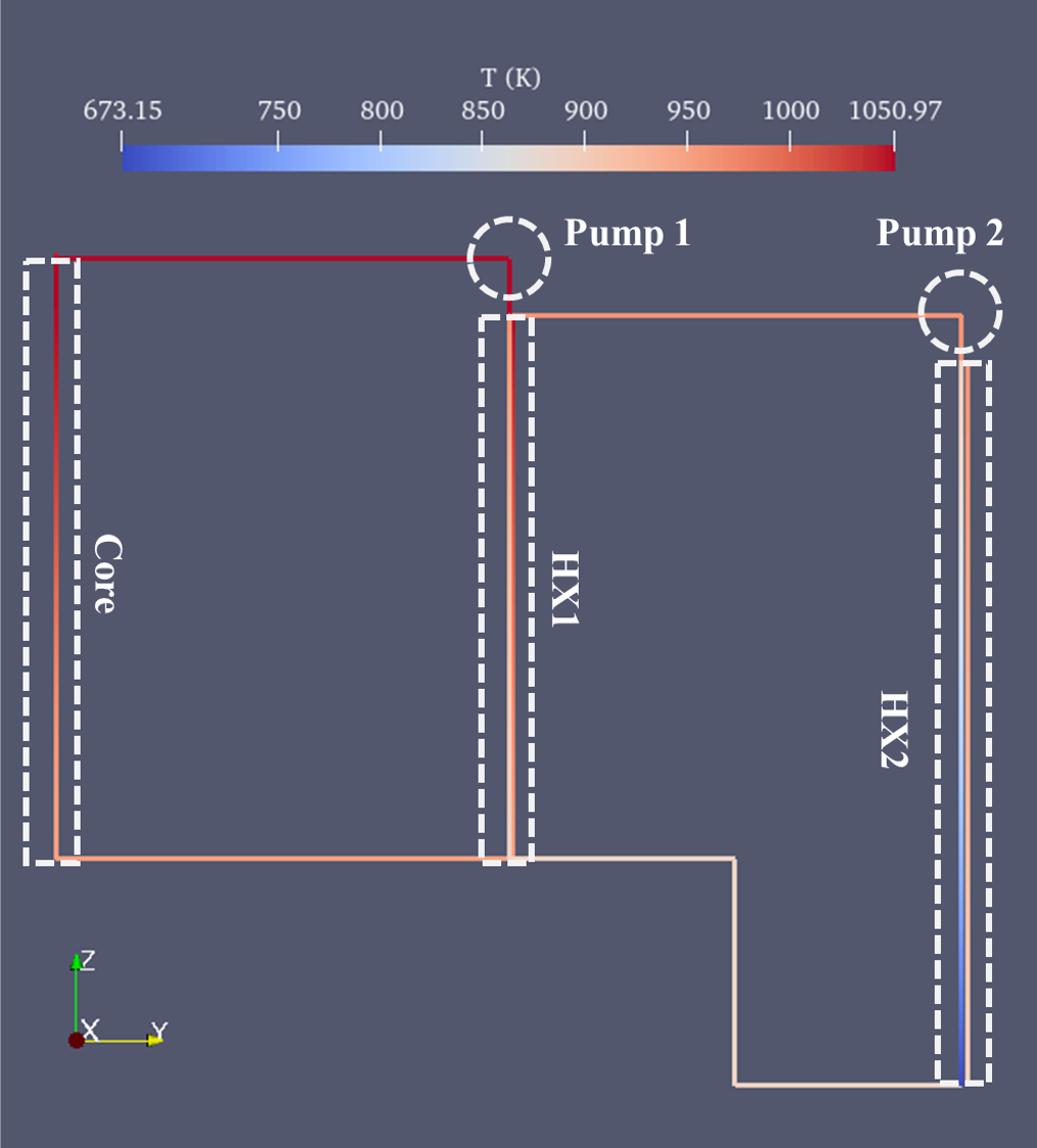
Figure 1: The steady-state temperature distribution in the 1-D MSRE primary loop (Pump1 and HX1 are primary pump and heat exchanger while Pump2 and HX2 are intermediate pump and heat exchanger).
Transient modeling
Two transient scenarios are considered here for the standalone 1-D MSFR SAM model:
pump head loss for the primary pump in ,
Total pump trip of the primary pump in .
The transient cases were restarted from the steady-state solutions, and the pump head change is initiated at . The neutronics response is modeled by the Point Kinetics Equations (PKE). As shown in Figure 2, right after the change in primary pump head, the fuel mass flow rate started to decrease. For the transient case of pump head loss, a new steady state was reached at the original mass flow rate. As for the case of total pump trip, the fuel mass flow rate drops significantly and the new converged mass flow rate is only the original value. Under the new steady-state after the pump trip, natural circulation becomes the dominant mechanism to drive the fuel circulation of primary circuit.
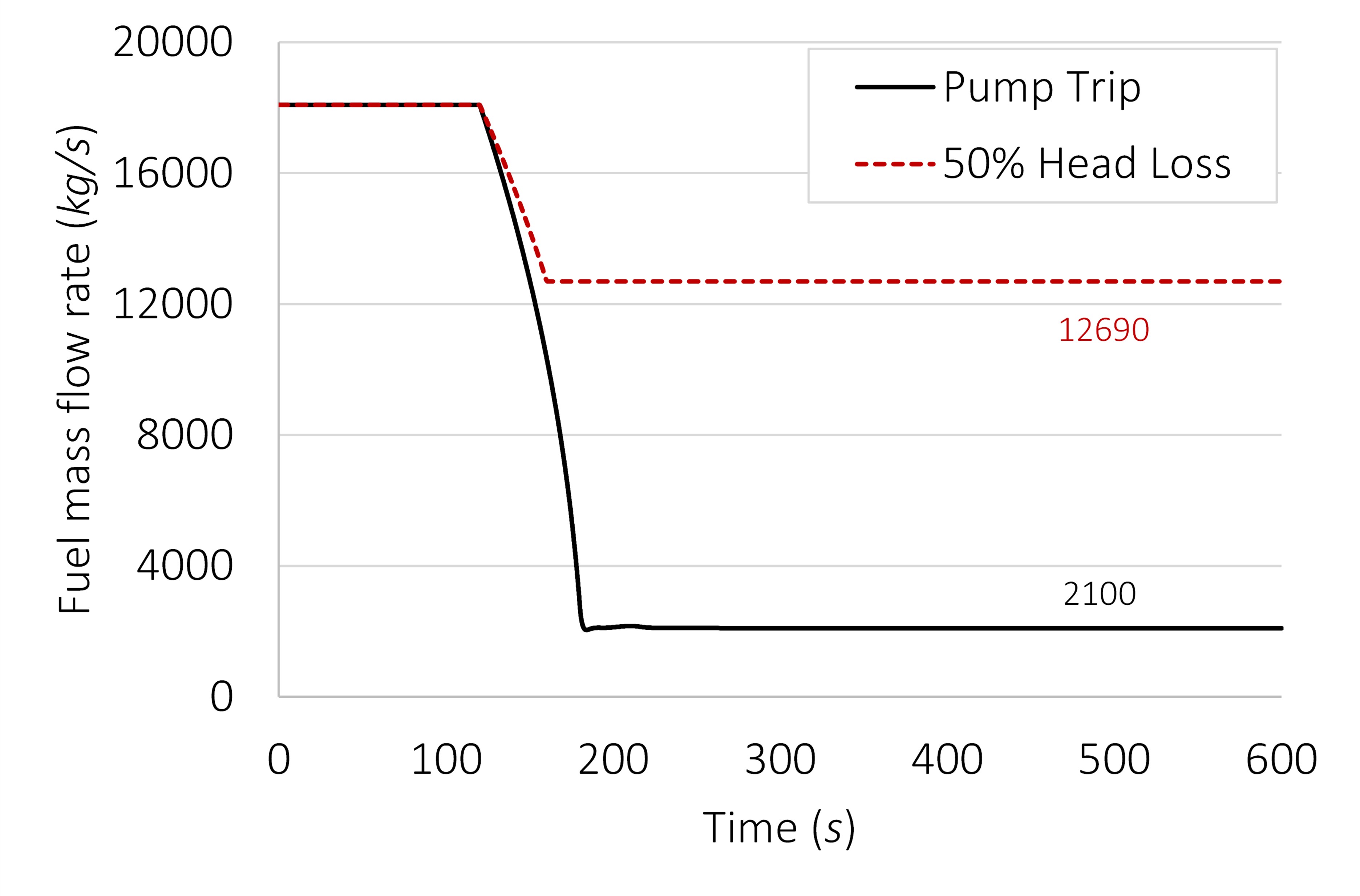
Figure 2: Evolution of fuel mass flow rates during the investigated transient scenarios.
Meanwhile, due to slower mass flow rate, the fuel is heated for longer period of time inside the core. As a result, the core outlet temperature started to rise after the pump head drop as shown in Figure 3. For the case of pump head loss, the core outlet temperature is observed to be higher than that with normal operating condition. While with the total pump trip, the core outlet temperature can be higher. Due to the negative temperature feedback coefficient, the reactor power decreases as the core temperature rises. As shown in Figure 4, the reactor power drops about when the primary pump loses half of its capacity, and about when the primary pump stops working. This well demonstrates the passive safety of MSFR design. The corresponding temperature rise along the core is for pump head loss scenario and for the pump trip case.
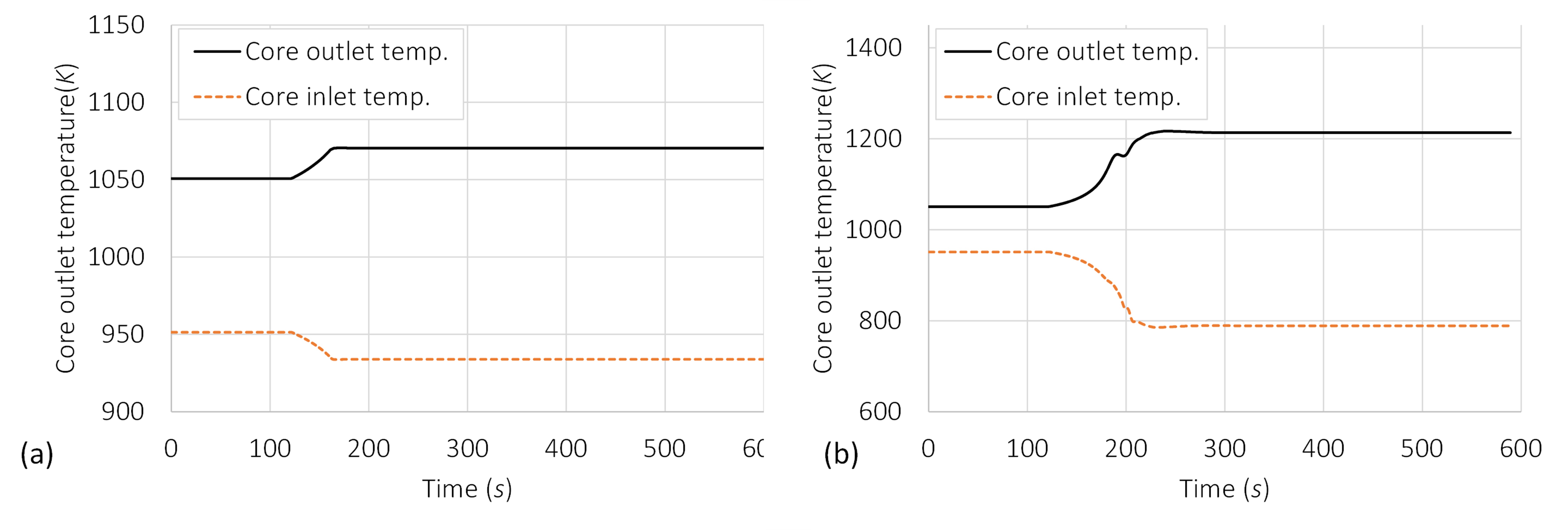
Figure 3: Evolution of core inlet and outlet temperatures during the investigated transient scenarios: (a) 50% pump head loss, (b) pump trip.
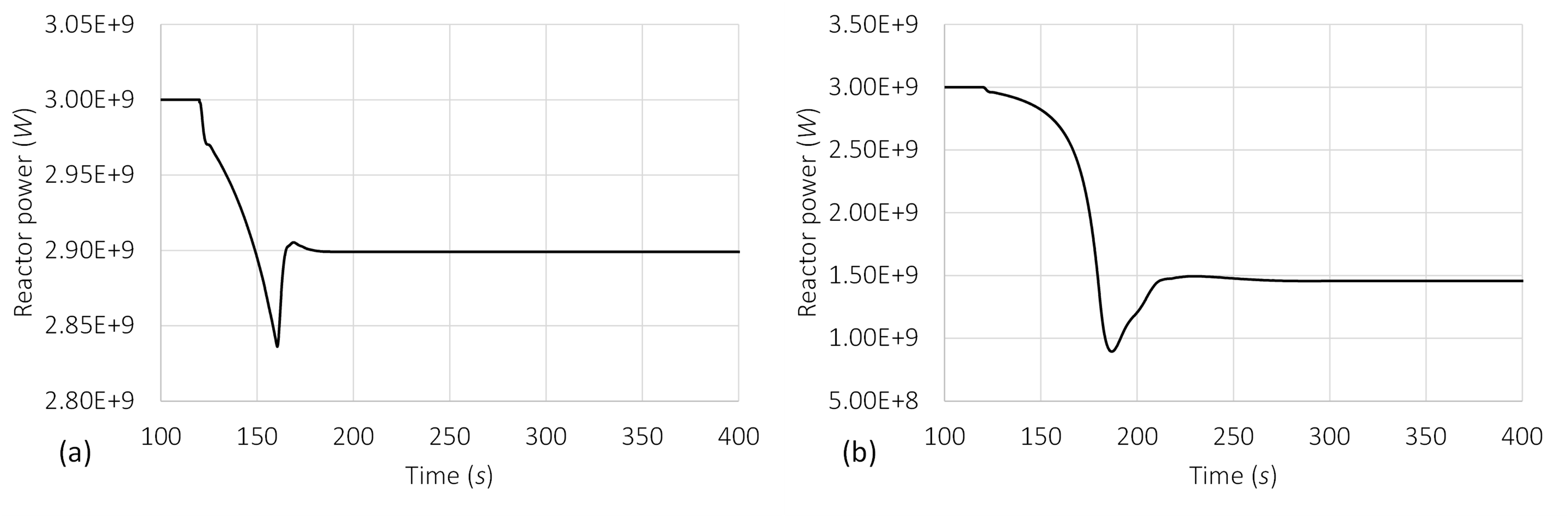
Figure 4: Evolution of reactor power during the investigated transient scenarios: (a) 50% pump head loss, (b) pump trip.
Input Description
The SAM input file adopts a block structured syntax, and each block contains the detailed settings of specific SAM components. In this section, we will go through all the important blocks in the input file and explain the key model specifications.
GlobalParams
This block contains the global parameters that are applied to all SAM components, such as the initial pressure, velocity, and temperature and the scaling for the solid temperature variables. A snippet is illustrated below:
  global_init_P = 1e5 # Initial pressure
  global_init_V = 0.01 # Initial velocity
  global_init_T = 898.15 # Initial temperature
  Tsolid_sf     = 1e-3 # Scaling factor for solid temperature variable
EOS (Equations of State)
This block specifies the material properties, such as the thermophysical properties. These ones include the fuel salt, intermediate loop salt, and pressurized helium in the secondary loop.
SAM supports both constants and user-defined functions for the thermophysical parameters in the EOS. The properties of common materials are implemented in the SAM repository, and can be readily used by simply referring to the material IDs, such as the air, or molten salt FLiBe.
[EOS]
  [fuel_salt_eos]
    type = PTFunctionsEOS
    rho = fuel_salt_rho_func
    cp = fuel_salt_cp_func
    mu = fuel_salt_mu_func
    k = fuel_salt_k_func
    T_max = 1200
    T_min = 800
    T_nodes = 21
    h_0 = 890400
  []
  [hx_salt_eos]
    type = SaltEquationOfState
    salt_type = Flibe
  []
  [Helium]
    type = HeEquationOfState
  []
[]
Components
This is the most important block that defines all the reactor components represented in the MSRE primary loop, such as the core, the heat exchanger, the pump, and all the connecting pipes. The Table below lists all the reactor components considered
Table 5: The reactor components represented in MSRE primary loop.
| Loop | Component | ID | Description |
|---|---|---|---|
| Primary Loop | Core | MSFR_core | The MSFR core |
| Primary Loop | Pipe 1 | pipe1 | Pipe from reactor core to primary heat excahnger |
| Primary Loop | Pipe 2 | pipe2 | Outlet pipe from the reactor core |
| Primary Loop | Pump 1 | pump | Primary loop pump |
| Primary Loop | HX1 | IHX1 | Primary-to-intermediate heat exchanger |
| Primary Loop | HX1 Primary Pipe | IHX1:primary_pipe | Pipe on the primary side of HX1 |
| Primary Loop | Pipe 3 | pipe3 | Pipe from HX1 output to reactor core inlet |
| Intermediate Loop | HX1 Secondary Pipe | IHX1:secondary_pipe | Pipe on the secondary side of HX1 |
| Intermediate Loop | Pipe 4 | pipe4 | Outlet pipe from HX1 on the secondary side |
| Primary Loop | Pump 2 | pump2 | Intermediate loop pump |
| Intermediate Loop | HX2 | IHX2 | Intermediate-to-secondary heat exchanger |
| Intermediate Loop | Pipe 5 | pipe5 | Admission pipe into HX2 |
| Intermediate Loop | HX2 Primary Pipe | IHX2:primary_pipe | Pipe on the primary side of HX2 |
| Intermediate Loop | Pipe 6 | pipe6 | Outlet pipe from HX2 on the primary side |
| Intermediate Loop | Pipe 7 | pipe7 | Pipe connecting pipe 6 and pipe 8 |
| Intermediate Loop | Pipe 8 | pipe8 | Admission pipe into HX1 on the secondary side |
| Secondary Loop | HX2 Secondary Pipe | IHX2:secondary_pipe | Pipe on the secondary side of HX2 |
As for the counter-flow, primary-to-intermediate shell-and-tube heat exchanger, both sides are modeled with 1-D channel components. The heat is exchanged through the 1-D wall coupling the shell and tube sides. A similar model is used for the secondary heat exchanger, except that pressurized Helium is used in the secondary side instead of salt.
[Components]
  [J_P2_IHX1]
    type = PBBranch
    inputs = 'pipe2(out)'
    outputs = 'IHX1(primary_in) '
    eos = fuel_salt_eos
    K = '1. 1.'
    Area = 2.24
  []
[]
[Components]
  [J_P5_IHX2]
    type = PBBranch
    inputs = 'pipe5(out)'
    outputs = 'IHX2(primary_in)'
    eos = hx_salt_eos
    K = '1. 1.'
    Area = 3.6
  []
[]
The primary pump is placed between between the outlet to the core and the primary heat exchanger. The input parameters for the primary and intermediate circuits pumps are specified here below:
[Components]
  [pump]
    type = PBPump
    Area = 2.24
    K = '0.15 0.1'
    eos = fuel_salt_eos
    inputs = 'pipe1(out)'
    outputs = 'pipe2(in)'
    initial_P = 1.0e5
    Head = 156010.45
  []
[]
[Components]
  [pump2]
    type = PBPump
    Area = 3.6
    K = '0.15 0.1'
    eos = hx_salt_eos
    inputs = 'pipe7(out)'
    outputs = 'pipe8(in)'
    initial_P = 1.0e5
    Head = 1.76e5
  []
[]
The detailed instructions of these SAM components can be found in the SAM user manual, which are not repeated here for brevity.
Postprocessors
The Postprocessors block is used to monitor the SAM solutions during the simulations, and quantities of interest can be printed out in the log file. For example, to check out the core outlet temperature, one can add the following snippet:
[Postprocessors]
  [Core_T_out]
    type = ComponentBoundaryVariableValue
    variable = temperature
    input = MSFR_core(out)
  []
[]
Preconditioning
This block describes the preconditioner used by the solver. New user can leave this block unchanged.
[Preconditioning]
  [SMP_PJFNK]
    type = SMP
    full = true
    solve_type = 'PJFNK'
    petsc_options_iname = '-pc_type -ksp_gmres_restart'
    petsc_options_value = 'lu 101'
    nl_sys = 'nl0'
  []
  [SMP_species]
    type = SMP
    full = true
    solve_type = 'PJFNK'
    petsc_options_iname = '-pc_type -ksp_gmres_restart'
    petsc_options_value = 'lu 101'
    nl_sys = 'species'
  []
[]Executioner
This block describes the calculation process flow. The user can specify the start time, end time, time step size for the simulation. Other inputs in this block include PETSc solver options, convergence tolerance, quadrature for elements, etc., which can be left unchanged.
[Executioner]
  type = SAMSegregatedTransient
  nl_systems_to_solve = 'nl0 species'
  [TimeStepper]
    type = FunctionDT
    function = TimeStepperFunc
    min_dt = 1e-3
  []
  nl_rel_tol = 1e-8
  nl_abs_tol = 1e-6
  nl_max_its = 25
  l_tol = 1e-6
  l_max_its = 200
  start_time = -1000
  end_time = 0.0
  num_steps = 20000
  [Quadrature]
    type = TRAP
    order = FIRST
  []
[]Modeling the transient conditions
Based upon the steady-state solutions, the transient simulations can be initiated by adjusting the primary pump head. A user defined function as shown below is used to linearly reduce the pump head from to in . Similar implementation is also applied in the pump trip modeling. Once the primary pump head changes, the MSFR SAM system model would start responding accordingly, and eventually new steady states are established with or original pump head.
[Functions]
  [head_func]
    # Dynamic pump head
    type = PiecewiseLinear
    x = '0   120 160  600'
    y = '1.0 1.0 0.5  0.5'
    scale_factor = 156010.45
  []
[][Components]
[pump]
type = PBPump
Area = 2.24
K = '0.15 0.1'
eos = fuel_salt_eos
inputs = 'pipe1(out)'
outputs = 'pipe2(in)'
initial_P = 1.0e5
Head = head_func
[]
[]Run Command
To run the related SAM system models, one can use the command below.
sam-opt -i msfr_1d_ss.i
The steady-state model has to be simulated before the transient modeling because the input files of transient models will use the checkpoint file from steady-state calculation as the initial condition.
References
- H. Rouch, O. Geoffroy, P. Rubiolo, A. Laureau, M. Brovchenko, D. Heuer, and E. Merle-Lucotte.
Preliminary thermal–hydraulic core design of the molten salt fast reactor (msfr).
Annals of Nuclear Energy, 64:449–456, 2014.
doi:10.1016/j.anucene.2013.09.012.[BibTeX]
@article{rouch2014,
    author = "Rouch, H. and Geoffroy, O. and Rubiolo, P. and Laureau, A. and Brovchenko, M. and Heuer, D. and Merle-Lucotte, E.",
    title = "Preliminary thermal–hydraulic core design of the Molten Salt Fast Reactor (MSFR)",
    journal = "Annals of Nuclear Energy",
    volume = "64",
    pages = "449-456",
    year = "2014",
    doi = "10.1016/j.anucene.2013.09.012"
}
(msr/msfr/plant/standalone_sam_model/msfr_1d_ss.i)
################################################################################
## Molten Salt Fast Reactor - Euratom EVOL + Rosatom MARS Design              ##
## SAM system modeling of the steady state condition                          ##
## Relaxation towards steady state balance of plant model                     ##
################################################################################

[GlobalParams]
  global_init_P = 1e5
  global_init_V = 0.01
  global_init_T = 898.15
  Tsolid_sf     = 1e-3
  scaling_factor_var = '1 1e-3 1e-6'
  species_system_name = 'species'
[]

[Problem]
  nl_sys_names = 'nl0 species'
[]

[Functions]
  [fuel_salt_rho_func] # Linear fitting used by Rouch et al. 2014
    type = PiecewiseLinear
    x = '800 1200'
    y = '4277.96 3925.16'
  []
  [fuel_salt_cp_func]
    type = PiecewiseLinear
    x = '800 1200'
    y = '1113.00 2225.00'
  []
  [fuel_salt_k_func]
    type = PiecewiseLinear
    x = '800 1200'
    y = '0.995200 1.028800'
  []
  [fuel_salt_mu_func] # Nonlinear fitting used by Rouch et al. 2014
    type = PiecewiseLinear
    x = '       800         820         840         860         880         900
                920         940         960         980        1000        1020
               1040        1060        1080        1100        1120        1140
               1160        1180        1200'
    y = '2.3887E-02  2.1258E-02  1.9020E-02  1.7102E-02  1.5449E-02  1.4015E-02
         1.2767E-02  1.1673E-02  1.0711E-02  9.8609E-03  9.1066E-03  8.4347E-03
         7.8340E-03  7.2951E-03  6.8099E-03  6.3719E-03  5.9751E-03  5.6147E-03
         5.2865E-03  4.9868E-03  4.7124E-03'
  []
  [TimeStepperFunc]
    type = PiecewiseLinear
    x = '-1000   -998   -995   -990   -980    -950   -500  0.0'
    y = ' 0.05    0.1    0.2    0.5    1.0     5.0   25.0 25.0'
  []
[]

[EOS]
  [fuel_salt_eos]
    type    = PTFunctionsEOS
    rho     = fuel_salt_rho_func
    cp      = fuel_salt_cp_func
    mu      = fuel_salt_mu_func
    k       = fuel_salt_k_func
    T_max   = 1200
    T_min   = 800
    T_nodes = 21
    h_0     = 890400
  []
  [hx_salt_eos]
    type      = SaltEquationOfState
    salt_type = Flibe
  []
  [Helium]
    type = HeEquationOfState
  []
[]

[MaterialProperties]
  [alloy-mat] # Based on Hastelloy N alloy
    type = SolidMaterialProps
    k    = 23.6
    Cp   = 578
    rho  = 8.86e3
  []
[]

[Components]
  [reactor]
    type          = ReactorPower
    initial_power = 3e9
    pke           = 'point_kinetics_basic'
  []

  [point_kinetics_basic] #DNP info is from Petterson, 2016
    type                       = PointKinetics
    LAMBDA                     = 3.46402e-7
    lambda                     = '1.33104E-02 3.05427E-02 1.15179E-01 3.01152E-01 8.79376E-01 2.91303E+00'
    betai                      = '8.42817E-05 6.84616E-04 4.79796E-04 1.03883E-03 5.49185E-04 1.84087E-04'
    Moving_DNP_bypass_channels = 'MSFR_core'
    feedback_components        = 'MSFR_core'
    feedback_start_time        = 0
  []

  [MSFR_core]
    type                                = PBMoltenSaltChannel
    eos                                 = fuel_salt_eos
    orientation                         = '0 0 1'
    position                            = '0 0 0'
    A                                   = 3.4636
    Dh                                  = 2.1
    length                              = 2.65
    n_elems                             = 20
    power_fraction                      = '1.0'
    coolant_density_reactivity_feedback = True
    n_layers_coolant                    = 20
    coolant_reactivity_coefficients     = -5.87554E-06
  []

  [Core_Out_Branch]
    type    = PBBranch
    inputs  = 'MSFR_core(out)'
    outputs = 'pipe1(in) loop_pbc(in)'
    eos     = fuel_salt_eos
    K       = '4.25 4.25 500.'
    Area    = 2.24
  []

  [pipe1] # Horizontal hot channel
    type        = PBOneDFluidComponent
    eos         = fuel_salt_eos
    position    = '0 0 2.65'
    orientation = '0 1 0'

    A           = 2.24
    Dh          = 1.6888
    length      = 2.0
    n_elems     = 12
  []

  [loop_pbc]
    type        = PBOneDFluidComponent
    eos         = fuel_salt_eos
    position    = '0 0 2.65'
    orientation = '0 0 1'

    A           = 2.24
    Dh          = 1.6888
    length      = 0.025
    n_elems     = 1
  []

  [TDV1]
    type        = PBTDV
    input       = 'loop_pbc(out)'
    eos         = fuel_salt_eos
    p_bc        = 1.0e5
  []

  #
  # ====== pump ======
  #

  [pump]
    type      = PBPump
    Area      = 2.24
    K         = '0.15 0.1'
    eos       = fuel_salt_eos
    inputs    = 'pipe1(out)'
    outputs   = 'pipe2(in)'
    initial_P = 1.0e5
    Head      = 156010.45
  []

  [pipe2] # Vertical hot channel from pump to HX
    type        = PBOneDFluidComponent
    eos         = fuel_salt_eos
    position    = '0 2.0 2.65'
    orientation = '0 0 -1'

    A           = 2.24
    Dh          = 1.6888
    length      = 0.25
    n_elems     = 3
  []

  [J_P2_IHX1]
    type    = PBBranch
    inputs  = 'pipe2(out)'
    outputs = 'IHX1(primary_in) '
    eos     = fuel_salt_eos
    K       = '1. 1.'
    Area    = 2.24
  []

  #
  # ====== Heat Exchanger ======
  #

  [IHX1]
    type                              = PBHeatExchanger
    eos                               = fuel_salt_eos
    eos_secondary                     = hx_salt_eos

    position                          = '0 2.0 2.4'
    orientation                       = '0 0 -1'
    A                                 = 2.24
    A_secondary                       = 3.60
    Dh                                = 0.02
    Dh_secondary                      = 0.0125
    length                            = 2.4
    n_elems                           = 24

    SC_HTC                            = 4
    HTC_geometry_type                 = Pipe
    HTC_geometry_type_secondary       = Pipe
    HT_surface_area_density           = 800.0
    HT_surface_area_density_secondary = 497.78

    initial_V_secondary               = -2.67
    Twall_init                        = 898.15
    wall_thickness                    = 0.001

    dim_wall                          = 1
    material_wall                     = alloy-mat
    n_wall_elems                      = 2
  []

  #
  # ====== Heat Exchanger Secondary Side ======
  #

  [IHX1_P3]
    type    = PBBranch
    inputs  = 'IHX1(primary_out)'
    outputs = 'pipe3(in) '
    eos     = fuel_salt_eos
    K       = '1. 1.'
    Area    = 2.24
  []

  [pipe3] # Horizontal cold channel
    type        = PBOneDFluidComponent
    eos         = fuel_salt_eos
    position    = '0 2.0 0.'
    orientation = '0 -1 0'

    A           = 2.24
    Dh          = 1.6888
    length      = 2.0
    n_elems     = 12
  []

  [Core_In_Branch]
    type    = PBBranch
    inputs  = 'pipe3(out)'
    outputs = 'MSFR_core(in)'
    eos     = fuel_salt_eos
    K       = '4.25 4.25'
    Area    = 2.24
  []

  #
  # ====== Intermediate circuit connected to HX1 ======
  #

  [IHX1_P4]
    type    = PBBranch
    inputs  = 'IHX1(secondary_out)'
    outputs = 'pipe4(in), loop2_pbc(in)'
    eos     = hx_salt_eos
    K       = '4.25 4.25 500.'
    Area    = 3.6
  []

  [loop2_pbc]
    type        = PBOneDFluidComponent
    eos         = hx_salt_eos
    position    = '0 2.0 2.4'
    orientation = '1 0 0'

    A           = 3.6
    Dh          = 2.14
    length      = 0.025
    n_elems     = 1
  []

  [loop2_TDV1]
    type        = PBTDV
    input       = 'loop2_pbc(out)'
    eos         = hx_salt_eos
    p_bc        = 1.0e5
  []

  [pipe4] # Horizontal intermediate hot leg
    type        = PBOneDFluidComponent
    eos         = hx_salt_eos
    position    = '0 2.0 2.4'
    orientation = '0 1 0'

    A           = 3.6
    Dh          = 2.14
    length      = 2.0
    n_elems     = 10
  []

  [J_P4_P5]
    type    = PBBranch
    inputs  = 'pipe4(out)'
    outputs = 'pipe5(in)'
    eos     = hx_salt_eos
    K       = '1. 1.'
    Area    = 3.6
  []

  [pipe5] # Vertical intermediate hot leg
    type        = PBOneDFluidComponent
    eos         = hx_salt_eos
    position    = '0 4.0 2.4'
    orientation = '0 0 -1'

    A           = 3.6
    Dh          = 2.14
    length      = 0.2
    n_elems     = 2
  []

  [J_P5_IHX2]
    type    = PBBranch
    inputs  = 'pipe5(out)'
    outputs = 'IHX2(primary_in)'
    eos     = hx_salt_eos
    K       = '1. 1.'
    Area    = 3.6
  []

  [IHX2]
    type                              = PBHeatExchanger
    eos                               = hx_salt_eos
    eos_secondary                     = Helium

    position                          = '0 4.0 2.2'
    orientation                       = '0 0 -1'
    A                                 = 2.4
    A_secondary                       = 7.2
    Dh                                = 0.04
    Dh_secondary                      = 0.01
    length                            = 3.2
    n_elems                           = 24

    SC_HTC                            = 4
    HTC_geometry_type                 = Pipe
    HTC_geometry_type_secondary       = Pipe
    HT_surface_area_density           = 510.0
    HT_surface_area_density_secondary = 170.0

    initial_V_secondary               = -50
    Twall_init                        = 900
    wall_thickness                    = 0.002

    dim_wall                          = 1
    material_wall                     = alloy-mat
    n_wall_elems                      = 2
  []

  [IHX2_S_In]
    type  = PBTDJ
    input = 'IHX2(secondary_in)'
    eos   = Helium
    v_bc  = -66.65
    T_bc  = 673.15
  []

  [IHX2_S_Out]
    type  = PBTDV
    input = 'IHX2(secondary_out)'
    eos   = Helium
    p_bc  = 7.5e6
  []

  [J_IHX2_P6]
    type    = PBBranch
    inputs  = 'IHX2(primary_out)'
    outputs = 'pipe6(in)'
    eos     = hx_salt_eos
    K       = '1. 1.'
    Area    = 3.6
  []

  [pipe6] # Intermediate cold leg
    type        = PBOneDFluidComponent
    eos         = hx_salt_eos
    position    = '0 4.0 -1.0'
    orientation = '0 -1 0'

    A           = 3.6
    Dh          = 2.14
    length      = 1.0
    n_elems     = 5
  []

  [J_P6_P7]
    type    = PBBranch
    inputs  = 'pipe6(out)'
    outputs = 'pipe7(in)'
    eos     = hx_salt_eos
    K       = '1. 1.'
    Area    = 3.6
  []

  [pipe7] # Intermediate cold leg
    type        = PBOneDFluidComponent
    eos         = hx_salt_eos
    position    = '0 3.0 -1.0'
    orientation = '0 0 1'

    A           = 3.6
    Dh          = 2.14
    length      = 1.0
    n_elems     = 5
  []

  [pump2]
    type      = PBPump
    Area      = 3.6
    K         = '0.15 0.1'
    eos       = hx_salt_eos
    inputs    = 'pipe7(out)'
    outputs   = 'pipe8(in)'
    initial_P = 1.0e5
    Head      = 1.76e5
  []

  [pipe8] # Intermediate cold leg
    type        = PBOneDFluidComponent
    eos         = hx_salt_eos
    position    = '0 3.0 0.0'
    orientation = '0 -1 0'

    A           = 3.6
    Dh          = 2.14
    length      = 1.0
    n_elems     = 5
  []

  [P8_IHX1]
    type    = PBBranch
    inputs  = 'pipe8(out)'
    outputs = 'IHX1(secondary_in)'
    eos     = hx_salt_eos
    K       = '1. 1.'
    Area    = 3.6
  []
[]

[Postprocessors]
  [Power]
    type = ScalarVariable
    variable = reactor:power
  []
  [Core_P_out]
    type     = ComponentBoundaryVariableValue
    variable = pressure
    input    = MSFR_core(out)
  []
  [Core_T_out]
    type     = ComponentBoundaryVariableValue
    variable = temperature
    input    = MSFR_core(out)
  []
  [Fuel_mass_flow] # Output mass flow rate at inlet of CH1
    type = ComponentBoundaryFlow
    input = MSFR_core(in)
  []
  [Core_T_in]
    type     = ComponentBoundaryVariableValue
    variable = temperature
    input    = MSFR_core(in)
  []
  [Core_P_in]
    type     = ComponentBoundaryVariableValue
    variable = pressure
    input    = MSFR_core(in)
  []

  [HX_Tin_p]
    type     = ComponentBoundaryVariableValue
    variable = temperature
    input    = IHX1(primary_in)
  []
  [HX_Tout_p]
    type     = ComponentBoundaryVariableValue
    variable = temperature
    input    = IHX1(primary_out)
  []
  [HX_Tout_s]
    type     = ComponentBoundaryVariableValue
    variable = temperature
    input    = IHX1(secondary_out)
  []
  [HX_Uout_s]
    type     = ComponentBoundaryVariableValue
    variable = velocity
    input    = IHX1(secondary_out)
  []
  [FliBe_mass_flow]
    type = ComponentBoundaryFlow
    input = IHX1(secondary_in)
  []
  [HX_Pin_s]
    type     = ComponentBoundaryVariableValue
    variable = pressure
    input    = IHX1(secondary_in)
  []

  [FliBe_mass_flow2]
    type = ComponentBoundaryFlow
    input = IHX2(primary_in)
  []
  [Gas_mass_flow]
    type = ComponentBoundaryFlow
    input = IHX2(secondary_in)
  []
  [HX2_Tin_p]
    type     = ComponentBoundaryVariableValue
    variable = temperature
    input    = IHX2(primary_in)
  []
  [HX2_Tout_p]
    type     = ComponentBoundaryVariableValue
    variable = temperature
    input    = IHX2(primary_out)
  []
  [HX2_Tout_s]
    type     = ComponentBoundaryVariableValue
    variable = temperature
    input    = IHX2(secondary_out)
  []
[]

[Preconditioning]
  [SMP_PJFNK]
    type                = SMP
    full                = true
    solve_type          = 'PJFNK'
    petsc_options_iname = '-pc_type -ksp_gmres_restart'
    petsc_options_value = 'lu 101'
    nl_sys              = 'nl0'
  []
  [SMP_species]
    type                = SMP
    full                = true
    solve_type          = 'PJFNK'
    petsc_options_iname = '-pc_type -ksp_gmres_restart'
    petsc_options_value = 'lu 101'
    nl_sys              = 'species'
  []
[]

[Executioner]
  type       = SAMSegregatedTransient
  nl_systems_to_solve = 'nl0 species'
  [TimeStepper]
    type     = FunctionDT
    function = TimeStepperFunc
    min_dt   = 1e-3
  []
  nl_rel_tol = 1e-8
  nl_abs_tol = 1e-6
  nl_max_its = 25
  l_tol      = 1e-6
  l_max_its  = 200
  start_time = -1000
  end_time   = 0.0
  num_steps  = 20000
  [Quadrature]
    type  = TRAP
    order = FIRST
  []
[]

[Outputs]
  print_linear_residuals = false
  perf_graph             = true
  [out_displaced]
    type          = Exodus
    use_displaced = true
    execute_on    = 'initial timestep_end'
    sequence      = false
  []
  [csv]
    type = CSV
    execute_scalars_on = 'none'
  []
  [checkpoint]
    type      = Checkpoint
    num_files = 1
  []
  [console]
    type               = Console
    execute_scalars_on = 'none'
  []
[]
(msr/msfr/plant/standalone_sam_model/msfr_1d_transient_01.i)
################################################################################
## Molten Salt Fast Reactor - Euratom EVOL + Rosatom MARS Design              ##
## SAM system modeling of 50% primary pump head loss                          ##
################################################################################

!include msfr_1d_ss.i

[Functions]
  [TimeStepperFunc]
    x := '0.0  100   120   160  200  240  300  600'
    y := '5.   5.    0.1   0.1    1.   1.   2.   2.'
  []
  [head_func] # Dynamic pump head
    type = PiecewiseLinear
    x    = '0   120 160  600'
    y    = '1.0 1.0 0.5  0.5'
    scale_factor = 156010.45
  []
[]

[Components]
  [point_kinetics_basic]
    feedback_start_time        := 120
  []

  [pump]
    Head   := head_func
  []
[]

[Problem]
  restart_file_base = msfr_1d_ss_checkpoint_cp/LATEST
[]

[Executioner]
  nl_max_its := 10
  start_time := 0.0
  end_time := 600
[]