Phase 2: Time-dependent Multiphysics Coupling
Description
This phase is composed of a sole task which aims to verify the multiphysics coupled transient calculations. The heat transfer coefficient is represented by a sinusoidal function of the following form (1) where is the reference volumetric heat transfer coefficient, and f is the frequency which results in a sinusoidal behavior of the reactor power. In the simulation, varying values of frequency used are 0.0125, 0.025, 0.05, 0.1, 0.2, 0.4, 0.8. The power gain in the reactor with the varying power can be calculated as a function of frequency according to the following equation
There are two coupled inputs for this stage. The first performs the neutronics calculations and the second performs the Navier-Stocks solution. The sinusoidal power behavior modeling is defined in the neutronics input as a function within the Functions module within the Navier-Stocks input.
[Functions]
  [alpha_val]
    type = ParsedFunction
    expression = '1.0e+6*(1.0 + 0.1*sin(2.0*pi*${frequency}*t))' #  'alpha_0*(1.0 + a*sin(fq*t))'
  []
[]For each frequency, 10 cycles are ran to obtain the asymptotic power wave. The last three cycles are used to obtain the power gain and phase shift. The problem is set to transient and the time step size is set inversely proportional to the frequency. This is requested in the Executioner block in the neutronics input as
[Executioner]
  type = Transient
  solve_type = PJFNK
  petsc_options_iname = '-pc_type -pc_factor_shift_type -pc_factor_mat_solver_package'
  petsc_options_value = 'lu NONZERO superlu_dist'

  start_time = 0.0
  dt = '${fparse max(0.005, 0.05*0.0125/frequency)}'
  end_time = '${fparse 10/frequency}'
  #[TimeStepper]
  #  type = IterationAdaptiveDT
  #  dt = 0.1
  #  growth_factor = 2
  #[]
  line_search = none #l2
  l_max_its = 200
  l_tol = 1e-3
  nl_max_its = 200
  nl_rel_tol = 1e-6
  nl_abs_tol = 1e-8

  # MultiApp iteration parameters
  fixed_point_min_its = 2
  fixed_point_max_its = 50
  fixed_point_rel_tol = 1e-6
  fixed_point_abs_tol = 1e-6
[]The rest of the transport solve input has a structure similar to that of the transport input in Step 1.3. The difference is in assigning a transient equation type instead of eigenvalue, and changing type input in Executioner block to Transient.
On the Navier-Stokes solve side, the problem is still executed as a transient solver. However, instead of running the problem for a long time to achieve steady state, the problem is defined as follows
[Executioner]
  type = Transient
  start_time = 0.0
  dt = '${fparse max(0.005, 0.05*0.0125/frequency)}'
  end_time = '${fparse 10/frequency}'
  #[TimeStepper]
  #  type = IterationAdaptiveDT
  #  dt = 0.1
  #  growth_factor = 2
  #[]
  solve_type = 'NEWTON'
  petsc_options_iname = '-pc_type -pc_factor_shift_type -pc_factor_mat_solver_package'
  petsc_options_value = 'lu NONZERO superlu_dist'
  line_search = l2 #'none'
  nl_rel_tol = 1e-6
  nl_abs_tol = 2e-8
  nl_max_its = 200
  l_max_its = 200
  automatic_scaling = true
[]Results
The results for this exercise report the power gain and the phase shift as a function of the frequency as defined above. The power gain decreases with increases the frequency, and the phase shift approaches 90 degrees with increasing the frequency. These results are displayed in Figure 1
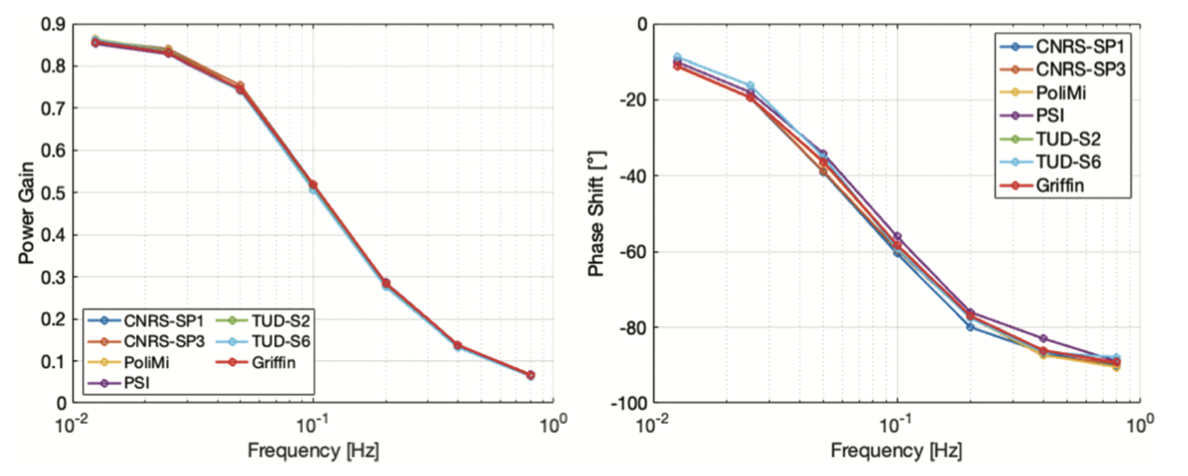
Figure 1: