HPMR-H_2 Reactor Results
Contact: Stefano Terlizzi sbt5572.at.psu.edu, Javier Ortensi javier.ortensi.at.inl.gov
Neutronics Verification
To verify the quality of the neutronics model, the Griffin and Serpent models are compared with a fixed temperature profiles (K, K, and ). With 1 polar and 3 azimuthal angles per octant (24 angles total), the Griffin eigenvalue error is 259 pcm and the relative error in power distributions for each assembly is given in Table 1 below.
Table 1: Error of power computed from Griffin vs. reference Serpent calculations for 20 axial layers and assemblies.
| Axial layer | Assembly 1 | Assembly 2 | Assembly 3 | Total |
|---|---|---|---|---|
| 1 | 0 | 0 | 0 | 0 |
| 2 | 0 | 0 | 0 | 0 |
| 3 | 2.87% | 3.33% | 2.40% | 2.89% |
| 4 | -2.63% | -2.96% | -3.80% | -3.10% |
| 5 | 0.58% | -0.45% | -1.34% | -0.35% |
| 6 | 0.61% | -0.55% | -1.38% | -0.39% |
| 7 | 0.93% | -0.50% | -1.38% | -0.26% |
| 8 | 1.21% | -0.37% | -1.38% | -0.11% |
| 9 | 1.36% | -0.24% | -1.37% | -0.01% |
| 10 | 1.47% | -0.22% | -1.18% | 0.09% |
| 11 | 1.56% | -0.23% | -1.18% | 0.12% |
| 12 | 1.43% | -0.11% | -1.15% | 0.12% |
| 13 | 1.56% | -0.11% | -1.18% | 0.16% |
| 14 | 1.38% | -0.19% | -1.26% | 0.04% |
| 15 | 1.23% | -0.12% | -1.19% | 0.04% |
| 16 | 1.22% | -0.01% | -1.11% | 0.11% |
| 18 | 3.10% | 2.79% | 1.55% | 2.54% |
| 19 | 0 | 0 | 0 | 0 |
| 20 | 0 | 0 | 0 | 0 |
| RMSE | 1.66% | 1.41% | 1.75% | 1.31% |
In that table, Assembly 1 is any of the center fuel assembly and Assemblies 2 and 3 correspond to any peripheral fuel assembly surrounded by 4 and 3 fuel assemblies, respectively. The relative errors in power are shown for each 10-cm thick axial layer of each assembly type and for all of them combined (Total), with axial layers 1 and 20 corresponding to the bottom and top of the core, respectively. The values are 0 for the top and bottom two layers because they do not contain any fissile material. The last row reports the Root Mean Square (RMSE) of the error in the corresponding assembly types.
Coupled Solution
Figure 1 (a) and (b) show the 3-D temperature and the stoichiometric ratio spatial distributions in the moderator pins, respectively. These figures reveal the stoichiometric ratio and moderator temperature to be inversely correlated. In fact, the hydrogen stoichiometric ratio increases when the moderator temperature decreases and vice-versa. This is further illustrated in Figure 1 (c), which reports the radially averaged moderator temperature and hydrogen concentration as a function of the distance from the bottom of the moderator pins.
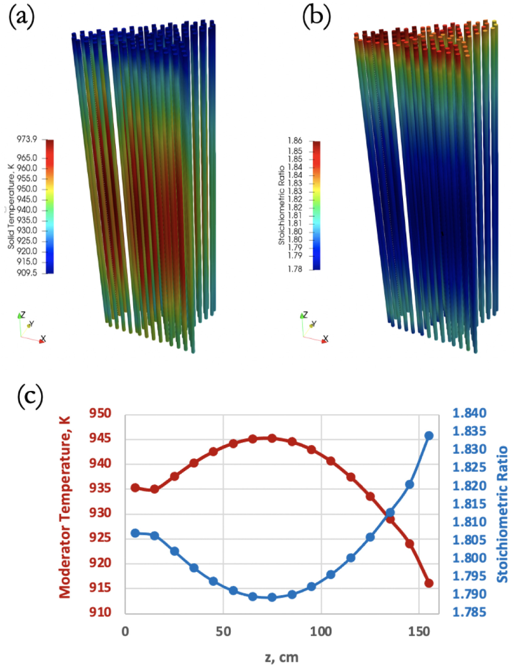
Figure 1: Three-dimensional temperature spatial distribution in the moderator pins, (b) 3-D hydrogen stoichiometric ratio spatial distribution, and (c) radially averaged moderator temperature and hydrogen stoichiometric ratio for 16 10-cm-high axial levels as a function of the distance from the bottom of the YHx moderator pins.
Table 2 reports the average, minimum, and maximum value for fuel temperature, denoted as , moderator temperature, , and, stoichiometric ratio, .
Table 2: Maximum, minimum, and average values for the fuel temperature, moderator temperature, and hydrogen stoichiometric ratio.
| Variable | Average | Minimum | Maximum |
|---|---|---|---|
| , K | 954.02 | 912.74 | 978.52 |
| , K | 947.83 | 911.11 | 973.84 |
| 1.8000 | 1.7769 | 1.8544 |
Table 3 below summarizes the global energy balance obtained with the model, showing a discrepancy of 0.04%.
Table 3: Summary of the global energy balance. The first three columns indicate the amount of the total power removed by the various boundaries. The last column reports the global energy balance discrepancy.
| Heat Pipe Condensers | Radial Boundary | Other Boundaries | Discrepancy |
|---|---|---|---|
| 98.00% | 2.03% | 0% | 0.04% |