Gas-cooled Microreactor Air Jacket: Nek5000 CFD Simulation

Contact: Anshuman Chaube (achaube.at.anl.gov), April Novak (anovak.at.anl.gov), Dillon Shaver (dshaver.at.anl.gov)

High Level Summary of Model

We have created a CFD model of a a gas-cooled microreactor air jacket cooling system that passively removes decay heat. The complex geometry and natural circulation-driven flow may be challenging to capture with systems-level codes without calibration from experiments or higher-fidelity thermal-fluid modelling. However, CFD is particularly well-suited to the task of modelling microreactor air jackets due to its ability to capture the effect of the complicated geometry on the flow with resolved boundary layers. We use Nek5000 to simulate flow through an industry-inspired prototypical geometry and predict heat transfer and flow characteristics. The boundary conditions given to us are representative of a reactor design in early stages of development. From these CFD simulations, it is possible to evaluate available models for bulk heat and momentum transfer that can be used in systems-level codes, and to develop modifications to those models specific to the proposed design. Given limited initial data, we can use CFD to fill in the gaps pertaining to systems-level quantities such as the friction factor, Nusselt number, the average heat flux, bulk temperature, and mean outlet temperature. The key idea here is to illustrate the utility of CFD in characterizing a newly developed system with greater accuracy than that achieved through systems-level codes and/or correlations-based analysis. We also aim to highlight the iterative improvement of the mass flow rate (varied as the Reynolds number) based on pressure and energy balance equations, which is the primary source of improvement over the results obtained using generic correlations. These equations in the workflow described below can be replaced by systems-levels tools or other software that can be used in conjunction with CFD in designing a microreactor.

We describe the geometry, the model setup, the fundamental equations used, and the boundary conditions of the CFD simulation. The results include the CFD solution as well as quantities of interest pertaining to systems-level modeling.

For our CFD simulations, we have used Nek5000 (ANL, 2019), which has been extensively validated and verified and used for many nuclear engineering applications. Nek5000 uses spectral element-based high-order spatial discretization, with second- and third-order time-stepping schemes available. It is highly scalable, and has capabilities for Direct Numerical Simulations, Large-Eddy Simulations, and unsteady Reynolds-Averaged Navier-Stokes (RANS) simulations.

Prerequisites

note

This tutorial assumes that you are familiar with the Nek5000 tutorial and have a general awareness of Nek5000's case structure, setup, and basic usage. You may ignore sections of the tutorial that focus on Nek5000's internal meshing utilities such as genbox, and instead use another meshing tool to generate a mesh in one of the two external formats supported by Nek5000 - an Exodus mesh (converted to Nek-supported .re2 using the exo2nek utility), or a Gmsh .msh mesh (converted to .re2 using gmsh2nek). Also consider skimming through the RANS Tutorial and the RANS example files to get better acquainted with the RANS models used in Nek5000.

Model Description, Theory, and Setup

Prior to explaining the workings of the CFD model, this section explains the theory underpinning our analysis. We discuss the advantages of using Nek5000 over conventional finite element CFD codes, followed by a look at the equations and the workflow we utilize in this analysis.

Nek5000 Theory

Nek5000 is a high-order CFD solver with its spatial discretization based on the Spectral Element Method(SEM) (Fischer and Tomboulides, 2023). The Nek5000 implementation of SEM uses high-order Legendre polynomials as basis functions and Gauss Lobatto Legendre points as SEM nodes. This allows for excellent convergence, stability, and low numerical dispersion. SEM offers key advantages over conventional finite-element solvers due to its ability to enable matrix-free forward operator evaluation using 1D stiffness matrices applied in succession, as opposed to forming full 2D or 3D stiffness matrices as in conventional finite-element solvers. This lowers floating-point operations and storage requirements for SEM significantly. For example, in 3D, the action of discrete operators can be evaluated with $var element = document.getElementById("moose-equation-da81596f-4f28-4bae-a01b-f03710fbab92");katex.render("O(EN^6)", element, {displayMode:false,throwOnError:false});$ work and using $var element = document.getElementById("moose-equation-e215f737-a4b5-406e-9db7-2fa1489321c2");katex.render("O(EN^3)", element, {displayMode:false,throwOnError:false});$ memory, which is respectively 2 and 1 order-of-magnitude lower than conventional finite elements (where $var element = document.getElementById("moose-equation-82b9ab2f-59f9-4e2d-807b-2212248ccd10");katex.render("E", element, {displayMode:false,throwOnError:false});$ is the number of elements, and $var element = document.getElementById("moose-equation-fa79b44e-b0d1-4c81-a6f4-4a137d780a85");katex.render("N", element, {displayMode:false,throwOnError:false});$ the number of unknowns in one dimension ).

This, however, limits the method to quadrilateral or hexahedral mesh elements, as 1D matrices need to be along clearly separable orthogonal axes for matrix-free forward operator evaluation. The trade off with using quad or hex elements is that care must be taken in meshing complex geometries to ensure elements conform well to non-linear features. Additionally, SEM's computational advantages come into play when one uses high-order elements. For that reason, Nek5000 runs best with elements of an order of at least 5, and ideally 7-11. Accordingly, if your prior experience is meshing for lower-order finite-elements, consider making a coarser mesh than usual and run the simulation at a high polynomial order, otherwise you are likely to end up with an over-resolved mesh, and any computational advantages of SEM will be nullified by the surplus degrees of freedom.

Nek5000 uses BDFk-EXTk solvers (Deville et al., 2002) that use extrapolation-based stabilization and implicit treatment of the advective term to provide second- to third-order time-stepping.

The main equations solved are

$(1)var element = document.getElementById("moose-equation-3770fe8e-3004-41d7-9318-f89eccde56f6");katex.render(" \\nabla\\cdot\\mathbf u=0", element, {displayMode:true,throwOnError:false});$

$(2)var element = document.getElementById("moose-equation-3b391737-01e5-447c-bdae-54959a120e36");katex.render(" \\rho_f\\left(\\frac{\\partial\\mathbf u}{\\partial t}+\\mathbf u\\cdot\\nabla\\mathbf u\\right)=-\\nabla P+\\nabla\\cdot\\tau+\\rho\\ \\mathbf f", element, {displayMode:true,throwOnError:false});$

$(3)var element = document.getElementById("moose-equation-02a6b502-5900-4ce7-bf44-135d41eed8c8");katex.render(" \\rho_f c_{p,f}\\left(\\frac{\\partial T_f}{\\partial t}+\\mathbf u\\cdot\\nabla T_f\\right)=\\nabla\\cdot\\left(k_f\\nabla T_f\\right)+\\dot{q}_f", element, {displayMode:true,throwOnError:false});$

Nek5000 is able to adjust its solver tolerances automatically and solve the equations above directly, working in what we refer to as the dimensional formulation. However, we often set up Nek5000 cases in the non-dimensional form, as Nek5000 solver tolerances are optimized for such a formulation.

The non-dimensionalised form of the Navier-Stokes equations is (Deville et al., 2002):

$(4)var element = document.getElementById("moose-equation-6670672d-998b-43f7-872b-305e608add55");katex.render(" \\tilde{\\nabla} \\cdot \\tilde{u} = 0 \\\\ \\frac{\\partial \\tilde{u}}{\\partial \\tilde{t}} + \\tilde{u} \\cdot \\tilde{\\nabla} \\tilde{u} = - \\tilde{\\nabla} \\tilde{p} + \\frac{1}{Re} \\tilde{\\nabla}^2 \\tilde{u} + \\tilde{F} \\\\ \\frac{\\partial \\theta}{\\partial \\tilde{t}} + \\tilde{u} \\cdot \\tilde{\\nabla} \\theta = \\frac{1}{Pe} \\tilde{\\nabla}^2 \\theta", element, {displayMode:true,throwOnError:false});$

where the non-dimensional temperature $var element = document.getElementById("moose-equation-2c06dbf2-b510-427e-b682-a38df88942f2");katex.render("\\theta", element, {displayMode:false,throwOnError:false});$ is based on a user-defined $var element = document.getElementById("moose-equation-00f10166-38b1-42c4-b342-6884b9843084");katex.render("T_0", element, {displayMode:false,throwOnError:false});$ and $var element = document.getElementById("moose-equation-c3314b41-6ca2-47c6-b201-901df4be43e9");katex.render("\\Delta T", element, {displayMode:false,throwOnError:false});$ : $(5)var element = document.getElementById("moose-equation-bad07ee5-86ba-4780-8c7c-75d68d2711d9");katex.render(" \\theta = \\frac{T-T_0}{\\Delta T}", element, {displayMode:true,throwOnError:false});$

note

When non-dimensionalizing, carefully consider the characteristic length-scale, characteristic velocity and reference temperatures based on estimated temperature and velocity values. Ideally, we want the maximum non-dimensional velocity and temperature to be as close to 1 as possible, and the respective minimum values to be 0.

To keep the computational costs for this tutorial accessible to as wide of a target audience as possible, we have used RANS to model turbulence. The RANS model used in our work is wall-resolved k- $var element = document.getElementById("moose-equation-5f91da60-a5fb-42f5-8df8-5d4bc0ecdf86");katex.render("\\tau", element, {displayMode:false,throwOnError:false});$ (Kok and Spekreijse, 2000). The advantages of $var element = document.getElementById("moose-equation-1babb3ed-fc93-4c77-b1ff-03193514d636");katex.render("k-\\tau", element, {displayMode:false,throwOnError:false});$ over $var element = document.getElementById("moose-equation-fa88bb43-11ea-4ade-8338-3b5b902dd38a");katex.render("k-\\epsilon", element, {displayMode:false,throwOnError:false});$ are similar to those of $var element = document.getElementById("moose-equation-bfaf08b1-7de0-4d45-ac68-07034fb9be19");katex.render("k-\\omega", element, {displayMode:false,throwOnError:false});$ , in that it is superior to $var element = document.getElementById("moose-equation-b0ac5c04-4ede-4642-929f-36263e858f58");katex.render("k-\\epsilon", element, {displayMode:false,throwOnError:false});$ in resolving the effects of near-wall behavior and the effects of streamwise pressure gradient. Additionally, it is more numerically stable than k- $var element = document.getElementById("moose-equation-0a609f2f-15bb-429f-957b-167a2f31ab40");katex.render("\\omega", element, {displayMode:false,throwOnError:false});$ as $var element = document.getElementById("moose-equation-6e7c8c12-52b1-4181-9eb8-d2530d719e76");katex.render("\\tau = 1/\\omega", element, {displayMode:false,throwOnError:false});$ , which simplifies wall boundary conditions to homogeneous Dirichlet conditions and creates well-bounded source terms for the $var element = document.getElementById("moose-equation-8dccdd86-686b-49cf-8e92-837d383fd5f2");katex.render("\\tau", element, {displayMode:false,throwOnError:false});$ scalar transport equation near the wall.

Air Jacket Geometry

The air jacket is a natural circulation driven passive heat removal component of a generic high-temperature gas-cooled microreactor. This "jacket" is the air gap between the reactor vessel and the shielding, as shown in Figure 1 (right). A wedge-shaped section of the fluid domain is shown in Figure 1 (left). The inner surface of the air gap is heated by the reactor vessel, whereas the outer surface is insulated. The inlet at the bottom supplies air at 50 $var element = document.getElementById("moose-equation-65c80425-b36c-46bc-a6ab-aace358c15f0");katex.render("^\\circ", element, {displayMode:false,throwOnError:false});$ C. The heated section, which is held at a constant temperature of 420 $var element = document.getElementById("moose-equation-01ebd855-3ba9-412b-ab01-30e4cf2db5e3");katex.render("^\\circ", element, {displayMode:false,throwOnError:false});$ C, drives the flow by natural circulation, causing the air to rise through the heated section before exiting at the exhaust at the top. The geometry that we have simulated is the 2D cross-section of a wedge-shaped slice of the air jacket.

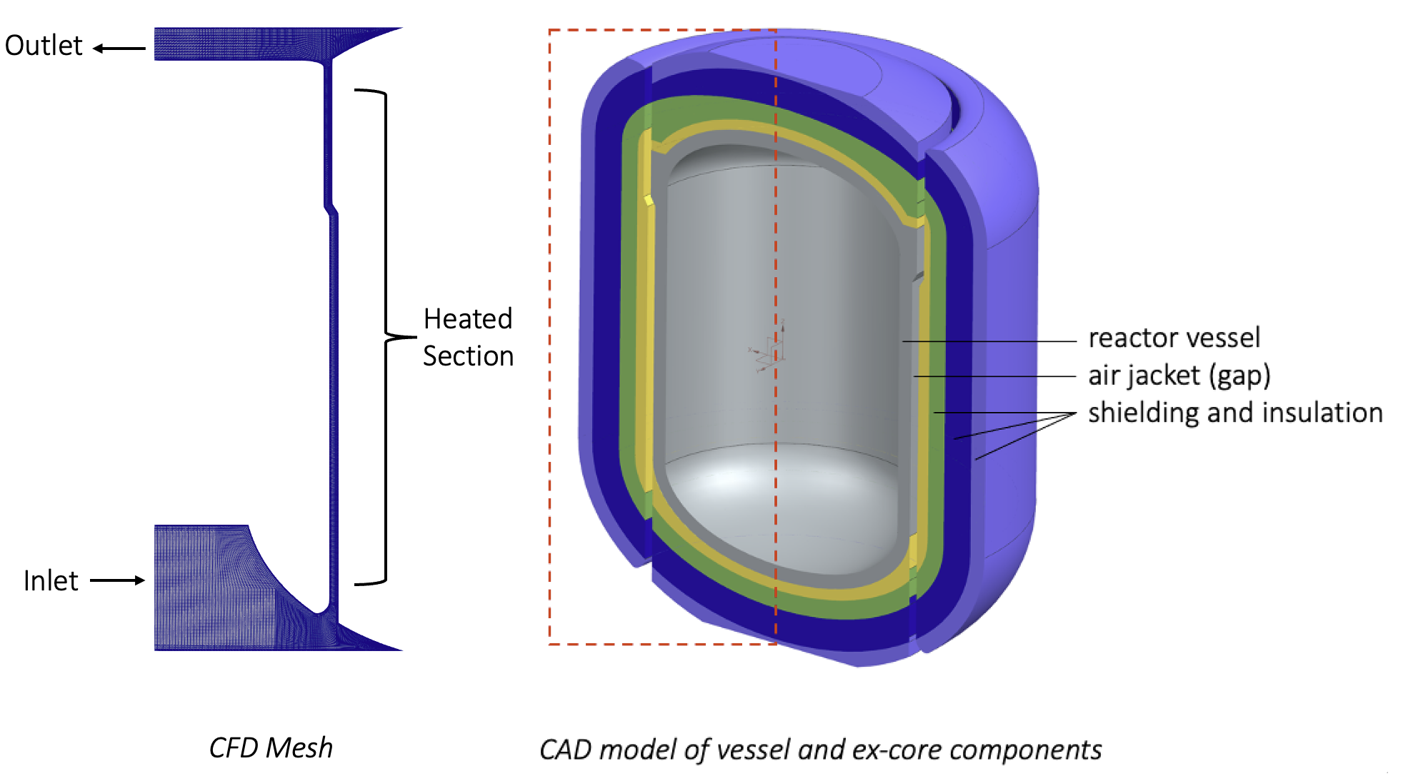
Figure 1: The microreactor core (right) and the air jacket geometry, meshed in 3D (left).

Pressure balance in natural circulation

A typical natural convection problem involves a closed loop with a heat source (usually heat flux boundary condition) and a heat sink. The problem here has an open loop that is representative of a nascent reactor design when the exact geometry is in flux and the heat sink and source are not precisely defined. Instead of a heat flux boundary condition, we are given a temperature Dirichlet condition which has a value equivalent to the maximum safe temperature of the hot wall, and we are asked to investigate the flow characteristics, friction factor, and heat transfer coefficient at said limiting condition.

The exact inlet boundary condition or the mass flow rate, and the outlet temperature are not known. However, based on the pressure balance expected for a natural convection problem, we can iteratively derive the mass flow rate, which can then be used to evaluate other quantities of interest.

To create a relatively inexpensive CFD model that is accessible to a wide range of users, we have chosen wall-resolved RANS as our turbulence model. The problem is essentially 2D in character, due to a lack of variation in CFD statistics in the azimuthal direction of the cylindrical air jacket domain after Reynolds-averaging. Hence a 2D simulation is adequate for the purposes of calculating flow and heat transfer characteristics for this geometry when using RANS. The problem is simulated in the axisymmetric mode to capture the cylindrical nature of the 3D geometry in relation to the 2D. The details of the axisymmetric mode setup are in the next section of the tutorial.

The effect of buoyancy is modeled using the simpler of two options available in Nek5000: the Boussinesq approximation, with air represented as an ideal gas, instead of the alternative, which is a low-Mach treatment with either ideal or real gas behavior (ANL, 2019). We are utilizing the simple gradient diffusion hypothesis to model the turbulent heat flux (Hsieh and Lien, 2004) with a turbulent Prandtl number of 0.85.

The density reduction as the air heats up in the air jacket creates the main buoyant pressure difference driving the natural circulation. The average density of air in the air jacket can be calculated during the simulation using the ideal gas law as a function of the mean temperature. Given temperature boundary conditions and dimensions, our main objective was to determine the friction factor and the Nusselt number ( $var element = document.getElementById("moose-equation-8c3c8009-2742-4b5e-93cb-2171e49591eb");katex.render("Nu", element, {displayMode:false,throwOnError:false});$ ). The pressure balance at the steady state is given by:

$(6)var element = document.getElementById("moose-equation-36e46058-8ab2-4209-a24d-5794be008ba9");katex.render(" \\Delta P_{int}= \\Delta P_{ext}", element, {displayMode:true,throwOnError:false});$

Assuming the inlet is at the ambient conditions, the external gravitational pressure drop is simply $var element = document.getElementById("moose-equation-9adf7eb4-b7cd-4bf4-a543-38471f456ecb");katex.render(" \\Delta P_{ext} = \\rho_0 g H", element, {displayMode:true,throwOnError:false});$ The total internal pressure drop includes the mean internal gravitational pressure drop and minor losses (with form and friction losses modeled with an effective friction factor) $var element = document.getElementById("moose-equation-d59acdbb-9130-4c2d-bb30-aaa75d49c874");katex.render(" \\Delta P_{int}= \\Delta P_{g}+\\Delta P_f", element, {displayMode:true,throwOnError:false});$ where the mean internal gravitational pressure drop (based on the mean weight of the air in the air jacket) and minor losses are modeled respectively as $(7)var element = document.getElementById("moose-equation-d4f6cf82-645b-4bcd-b759-4e266550a575");katex.render("\\Delta P_g = \\rho_m g H ", element, {displayMode:true,throwOnError:false});$ $var element = document.getElementById("moose-equation-ebd1132f-66f1-4bb4-879c-0ceabb69d86d");katex.render("\\Delta P_f = \\frac{1}{2} \\frac{f}{D} H \\rho_0 U_m ^2", element, {displayMode:true,throwOnError:false});$ Combining these with the total pressure balance given by Eq. (6) yields $var element = document.getElementById("moose-equation-87d7993d-ba8f-4c11-a7ac-5889e3366feb");katex.render(" \\frac{1}{2} \\frac{f}{D} H \\rho_0 U_m ^2+\\rho_m g H =\\rho_0 g H", element, {displayMode:true,throwOnError:false});$ $(8)var element = document.getElementById("moose-equation-2fefa2e8-129c-433d-af60-c4a738fe6b50");katex.render(" \\frac{1}{2} \\frac{f}{D} H \\rho_0 U_m ^2 =\\left(\\rho_0 -\\rho_m\\right) g H", element, {displayMode:true,throwOnError:false});$

Since the gravitational pressure drop is a hydrostatic quantity, we adopt "mean density" to imply volumetric mean (simple volumetric average) rather than bulk mean (velocity-weighted volumetric average). The mean density is then evaluated using the Boussinesq model and the ideal gas approximation ( $var element = document.getElementById("moose-equation-4ea0214b-d946-42af-8da7-e1f9d953a546");katex.render("\\beta_0 = 1/T_0)", element, {displayMode:false,throwOnError:false});$ . The general relationship for density is then given by $var element = document.getElementById("moose-equation-95c5d187-660b-4c47-895e-4eca0eebd930");katex.render(" \\rho - \\rho_0 = -\\rho_0\\beta_0\\left(T - T_0\\right)", element, {displayMode:true,throwOnError:false});$ Since this gives a linear relationship between density and temperature, we have $var element = document.getElementById("moose-equation-9ad923db-1cc1-4046-a544-8e2527fa9db5");katex.render(" \\rho_0 -\\rho_m = \\rho_0\\beta_0\\left(T_m-T_{in}\\right)", element, {displayMode:true,throwOnError:false});$ The pressure balance then becomes $(9)var element = document.getElementById("moose-equation-1f4ca14d-280d-4353-a382-3975c094402a");katex.render(" \\frac{1}{2} \\frac{f}{D} H \\rho_0 U_m ^2 =\\rho_0\\beta_0\\left(T_m-T_{in}\\right) g H", element, {displayMode:true,throwOnError:false});$

The friction factor can be obtained using $(10)var element = document.getElementById("moose-equation-c6df65d2-dfb0-4348-8830-54bfb32fdff5");katex.render(" f =\\frac{2Dg}{U_m ^2}\\beta_0\\left(T_m-T_0\\right)", element, {displayMode:true,throwOnError:false});$

Initial guess for velocity and mean temperature

Given the geometry, the inlet temperature, and the hot wall temperature, there are two main unknowns that we need to estimate: $var element = document.getElementById("moose-equation-c5be3359-4ad8-4d9e-81b5-bb2478f90041");katex.render("\\bar{U}", element, {displayMode:false,throwOnError:false});$ : the mean inlet velocity, which shall help us determine the Reynolds number of the simulation, and $var element = document.getElementById("moose-equation-0fb96ced-a16a-4d46-83c7-0447d5ae6221");katex.render("T_m", element, {displayMode:false,throwOnError:false});$ : the bulk temperature, that will help us understand the energy balance and define the Boussinesq acceleration term.

These two unknowns are coupled through pressure and energy balance equations. These equations involve the following quantities: $(11)var element = document.getElementById("moose-equation-aa7d25c1-1d7a-4a47-bf78-5e60c71924b8");katex.render(" T_{mean} = \\frac{1}{2} (T_o + T_{in})", element, {displayMode:true,throwOnError:false});$ $var element = document.getElementById("moose-equation-1d5b293e-ed25-40b1-bf2e-795cba088149");katex.render("\\rho_{mean} = \\frac{P_o M_{air}}{R T_{mean}}", element, {displayMode:true,throwOnError:false});$ $var element = document.getElementById("moose-equation-9d0384be-6ec9-42db-b7ea-8bc67e40d5b3");katex.render("Re = \\frac{\\rho_{mean} \\bar{U} D_h } {\\mu}", element, {displayMode:true,throwOnError:false});$ $var element = document.getElementById("moose-equation-104a5c98-e62b-46c7-a65e-982927785c9e");katex.render("f_D = 0.3164 Re^{-0.25}", element, {displayMode:true,throwOnError:false});$ $(12)var element = document.getElementById("moose-equation-98dbab1a-4e50-4d8d-a44e-8a91099dae85");katex.render("h = \\frac{k_f}{L} (0.023 Re^{0.8} Pr^{0.4}) ", element, {displayMode:true,throwOnError:false});$ where $var element = document.getElementById("moose-equation-73cd8f85-d291-477c-bd4a-7e42ddffc518");katex.render("P_o", element, {displayMode:false,throwOnError:false});$ is the atmospheric pressure, $var element = document.getElementById("moose-equation-d1e30313-bf9d-45fa-84b0-fcf12daf9957");katex.render("M_{air}", element, {displayMode:false,throwOnError:false});$ the molar mass of air (approx. 28 g mol $var element = document.getElementById("moose-equation-91ea88a2-42c1-4ad0-a7f1-c21c7ae777aa");katex.render("^{-1}", element, {displayMode:false,throwOnError:false});$ (Jones, 1978)), $var element = document.getElementById("moose-equation-801c8ed8-168b-4be7-9561-0de1ec1fd23a");katex.render("R", element, {displayMode:false,throwOnError:false});$ the gas constant, $var element = document.getElementById("moose-equation-afdccb20-da98-4787-bd47-a016893f01f6");katex.render("f_D", element, {displayMode:false,throwOnError:false});$ the Darcy friction factor, $var element = document.getElementById("moose-equation-13c4c6f2-a5fd-4a66-96dc-30dd44e86aef");katex.render("Re", element, {displayMode:false,throwOnError:false});$ the Reynolds number, and $var element = document.getElementById("moose-equation-7c86b0d6-276b-4db1-a972-a1cb28c6ed17");katex.render("Pr", element, {displayMode:false,throwOnError:false});$ the Prandtl number.

Note that we are assuming ideal gas behaviour, and are also neglecting the pressure differences within the domain relative to atmospheric pressure. The mean temperature is approximated as the mean of the inlet and outlet temperatures as an initial guess, and the outlet temperature is the independent unknown variable. The correlations for the friction factor and heat transfer coefficient assume turbulent flow. You may find other correlations to be more appropriate for your case, however the idea is to verify that the results obtained from the pressure and energy balance obtained later in this section are consistent with your assumptions and correlations. In this case, we will find that assuming the flow is not laminar is appropriate. Also note that the main unknowns are still $var element = document.getElementById("moose-equation-af717a38-3a66-449b-b138-2869a3519846");katex.render("\\bar{U}", element, {displayMode:false,throwOnError:false});$ and $var element = document.getElementById("moose-equation-d98f3e7d-6ffc-4d90-ac5a-664fb0da27d4");katex.render("T_m", element, {displayMode:false,throwOnError:false});$ or $var element = document.getElementById("moose-equation-e6f0c8d1-489d-4c47-811b-c59d67faa561");katex.render("T_o", element, {displayMode:false,throwOnError:false});$ , with Eq. (11)-Eq. (12) being secondary equations that will feed into our main pressure and energy balance equations.

The pressure balance equation has already been discussed (Eq. (9)). The energy balance is given by the balance between the convective heat transfer between the hot wall and the fluid bulk, and the heat advected into and out of the air jacket: $var element = document.getElementById("moose-equation-c5d053e2-5ddd-4152-bd19-83a687719caa");katex.render("q_{hot wall} = q_{advection}", element, {displayMode:true,throwOnError:false});$ $var element = document.getElementById("moose-equation-b9f2b7ad-e7fd-4a7d-a129-4396fb28f4ba");katex.render("A_{hw} h(T_{hot} - T_{mean}) = \\dot{m} C_p (T_o - T_{in})", element, {displayMode:true,throwOnError:false});$ $(13)var element = document.getElementById("moose-equation-80678e22-f1cd-4089-a0f8-e4e2cc002c3f");katex.render("A_{hw} h(T_{hot} - T_{mean}) = \\rho_{mean} \\bar{U} A_c C_p (T_o - T_{in}) ", element, {displayMode:true,throwOnError:false});$ where $var element = document.getElementById("moose-equation-175ac586-9262-4207-9606-4036f4620cfd");katex.render("A_{hw}", element, {displayMode:false,throwOnError:false});$ is the hot wall area, $var element = document.getElementById("moose-equation-e7e65bc9-facd-44e5-8580-01f95ac08ddf");katex.render("T_{hot}", element, {displayMode:false,throwOnError:false});$ the hot wall temperature, $var element = document.getElementById("moose-equation-4368bdb1-1575-4e1f-8547-1000ef082302");katex.render("A_c", element, {displayMode:false,throwOnError:false});$ the cross section area of the channel.

The main equations to be solved for $var element = document.getElementById("moose-equation-73795537-6843-4b43-852e-d7bb7b74c06a");katex.render("\\bar{U}", element, {displayMode:false,throwOnError:false});$ and $var element = document.getElementById("moose-equation-83953b33-58b3-4400-92e3-c24ad30cd0a6");katex.render("T_o", element, {displayMode:false,throwOnError:false});$ are Eq. (9) and Eq. (13). These are non-linear, and can be easily solved with symbolic mathematics software or iterative solver packages such as scipy.

def pqbalance(ubto):
    ub, to = ubto
    #turbulent:
    expr1 = (rho_amb*beta*(T_mean(to)-T_in)*g*H) - (fdturb(ub)*rho_amb*ub*ub*H/2.0/Dh)
    expr2 = (Ahot*htcoeff(ub)*(T_hot-T_mean(to))) - (rho_amb*ub*Aw*Cp*(to-T_in))

    return (expr1,expr2)

if (turbulent):
    #turbulent solve
    Ubar, Tout =  scp.optimize.fsolve(pqbalance, (1.0, 0.5*(T_hot+T_in)))

Approximations for $var element = document.getElementById("moose-equation-1bedb159-03bb-462e-86a1-6f5872f976d7");katex.render("T_m", element, {displayMode:false,throwOnError:false});$ (which require an approximate heat transfer coefficient $var element = document.getElementById("moose-equation-7455534d-399f-4b65-b1d2-5368cea13158");katex.render("h", element, {displayMode:false,throwOnError:false});$ ) and $var element = document.getElementById("moose-equation-6739d70c-36ff-43d0-aa48-2d7e038e65ea");katex.render("f", element, {displayMode:false,throwOnError:false});$ using conventional correlations (such as Dittus-Boelter and Blasius correlations, respectively) can be used for an initial guess, but as the simulation is run, values are calculated directly from the results. With these results, the correct $var element = document.getElementById("moose-equation-ad6951b4-aec3-4430-b96b-0885666cd348");katex.render("f", element, {displayMode:false,throwOnError:false});$ and $var element = document.getElementById("moose-equation-d78e07b0-af98-417e-9308-89a94d283486");katex.render("Nu", element, {displayMode:false,throwOnError:false});$ can be determined for a given $var element = document.getElementById("moose-equation-23fc6445-d63c-423b-b043-3c3647fe0843");katex.render("U_m", element, {displayMode:false,throwOnError:false});$ .

We have assumed uniform inlet ( $var element = document.getElementById("moose-equation-d72f220f-aaa0-4bfc-92eb-21ea75d2249a");katex.render("T_{in}", element, {displayMode:false,throwOnError:false});$ ) and hot-wall temperatures ( $var element = document.getElementById("moose-equation-3d46b251-0219-4c5c-913d-e460313643d8");katex.render("T_{wall}", element, {displayMode:false,throwOnError:false});$ ) based on simple data from limiting conditions, while all remaining walls have adiabatic boundary conditions applied to temperature due to insulating material.

The outlet was artificially extended by a few characteristic lengths and the Boussinesq acceleration term gradually ramped down to allow for the highly biased jet in the upper plenum to redistribute and flow outwards at the outlet uniformly in order to avoid any eddies that can cause numerical divergence-inducing backflow at the outlet. The gradual ramping down prevents any effect on the results upstream. Wall resolution was ensured by monitoring $var element = document.getElementById("moose-equation-ee00b970-642c-4977-b4be-f7408478f844");katex.render("y^+", element, {displayMode:false,throwOnError:false});$ 1 values at the first Gauss Lobatto Legendre point off the wall.

To capture the buoyant momentum source, we have applied the Boussinesq approximation. The Boussinesq term is a forcing term applied to the momentum Navier-Stokes Equation (Eq. (4)), which in non-dimensional terms, is expressed as $var element = document.getElementById("moose-equation-6db112b2-033e-4f74-a07a-dfe54d5669d6");katex.render("\\tilde{F} = \\frac{ \\beta_0 (T - T_0) g L}{U ^2} \\hat{z} = Ri \\: \\theta", element, {displayMode:true,throwOnError:false});$ where $var element = document.getElementById("moose-equation-8099e717-343a-40e0-9722-e837fe0821ea");katex.render("Ri", element, {displayMode:false,throwOnError:false});$ is the Richardson number, $var element = document.getElementById("moose-equation-af71c826-1a82-4623-800e-ac377e228ba2");katex.render("T", element, {displayMode:false,throwOnError:false});$ the dimensional local temperature, and $var element = document.getElementById("moose-equation-bfeded66-0c87-4cff-9c4d-779dbd3a9011");katex.render("\\theta", element, {displayMode:false,throwOnError:false});$ the non-dimensional local temperature.

The average Nusselt Number is calculated as $var element = document.getElementById("moose-equation-e28308f6-7c8d-4ea5-84b7-d86d5f29f6a7");katex.render("Nu = \\frac{hL}{k} = \\frac{L}{k} \\left( \\frac{k (\\nabla T |_{wall} \\cdot \\hat{n})}{T_w - T_b} \\right) = \\frac{\\tilde{\\nabla} \\theta | _{wall} \\cdot \\hat{n}}{\\theta _w - \\theta _b}", element, {displayMode:true,throwOnError:false});$ where $var element = document.getElementById("moose-equation-d59dfc9e-496a-41a7-ba8d-aefd3e9399a3");katex.render("\\tilde{\\nabla}\\theta | _{wall}", element, {displayMode:false,throwOnError:false});$ is the average non-dimensional temperature gradient at the hot wall, $var element = document.getElementById("moose-equation-443d97db-b246-4ce7-b677-598c6d3b3e87");katex.render("\\theta_w", element, {displayMode:false,throwOnError:false});$ the non-dimensional hot-wall temperature, and $var element = document.getElementById("moose-equation-6c6df564-4a09-484f-9ec1-19b7ffba690c");katex.render("\\theta_b", element, {displayMode:false,throwOnError:false});$ the non-dimensional fluid bulk temperature.

Once the simulation has attained a fully developed state, it is possible to compare the pressure drop calculated from the CFD simulation, say $var element = document.getElementById("moose-equation-5c5c2480-aab3-4575-9b7d-bfca72187791");katex.render("\\Delta P", element, {displayMode:false,throwOnError:false});$ , and compare it to the expected pressure drop based on Eq. (7), that is, zero (as the external pressure is balanced by the internal pressure at steady state). If the two pressure drops do not match, it is possible to iterate on the value of the mass flow rate by adjusting characteristic velocityu $var element = document.getElementById("moose-equation-386ebc5d-067f-4306-839f-81c26174c551");katex.render("U_m", element, {displayMode:false,throwOnError:false});$ , or in other words, the Reynolds number (Eq. (4)) until we arrive at the expected pressure drop, using the procedure described in Figure 2.

Figure 2: The iterative algorithm that can be used to derive the correct pressure drop according to Eq. (7).

Computational Model Description

The following section describes the input file and the model setup. Please note that the setup of the RANS model is identical to the Nek5000 RANS Channel tutorial mentioned in the introduction, and is therefore not repeated here for the sake of brevity.

Axisymmetric Mode Setup

In Nek5000, the axisymmetric mode requires the axis of symmetry to be the x-axis, which becomes the r-axis, while the y-axis becomes the vertical axis. Furthermore, the entire mesh must lie above the x-axis/r-axis, as there can be no negative r values. Your mesh needs to be oriented accordingly in your mesh generator. Mesh modifications can also be performed in Nek5000, in the usr file's usrdat2 function. For the air jacket mesh (Figure 1), the mesh needs to be rotated clockwise by 90 degrees to be aligned with the axis of symmetry. This is accomplished by the following code:

C     rescale the domain BEFORE calling rans_init

      theta = pi/2.0
      do i=1,n
        xx = xm1(i,1,1,1)
        yy = ym1(i,1,1,1)
        xm1(i,1,1,1) =  xx*cos(theta) + yy*sin(theta)
        ym1(i,1,1,1) = -xx*sin(theta) + yy*cos(theta)
      enddo

Once the mesh has the desired orientation, the axisymmetric mode can be turned on in the par file using the axiSymmetry = yes line in the [PROBLEMTYPE] block:

[PROBLEMTYPE]
equation = incompNS
axiSymmetry = yes

Boundary Conditions, Initial Conditions, Boussinesq approximation

Tying sidesets to a type of boundary condition can be accomplished through the par file. For each field, such as VELOCITY, sidesets starting from 1 can be assigned a boundary type using the boundaryTypeMap key:

[VELOCITY]
density = 1.0
viscosity = -3580.0
residualTol = 1e-6
boundaryTypeMap = v  ,O  ,W  ,W

A similar action can be accomplished in the usr file, in the usrdat2 routine, by modifying the cbc array. This is recommended when your sideset IDs have arbitrary numbers that do not start with 1

c     assign BCs to sidesets using cbc array
c      do e=1,nelv
c      do f=1,2*ndim
c        id_face = boundaryID(f,e)
c        if (id_face.eq.1) then        ! dirichlet (inlet)  BCs
c           cbc(f,e,1) = 'v  '
c           cbc(f,e,2) = 't  '
c        elseif (id_face.eq.2) then    ! Outlet
c           cbc(f,e,1) = 'O  '
c           cbc(f,e,2) = 'O  '
c        elseif (id_face.eq.3) then    ! Hot wall
c           cbc(f,e,1) = 'W  '
c           cbc(f,e,2) = 't  '
c        elseif (id_face.eq.4) then    ! Insulated wall
c           cbc(f,e,1) = 'W  '
c           cbc(f,e,2) = 'I  '
c        endif
c      enddo

The inlet boundary has a constant $var element = document.getElementById("moose-equation-2fb20e2f-4792-485f-955c-6c1751f0b111");katex.render("u_x", element, {displayMode:false,throwOnError:false});$ , $var element = document.getElementById("moose-equation-9594774a-113f-4205-965c-472ec639334c");katex.render("u_y", element, {displayMode:false,throwOnError:false});$ , $var element = document.getElementById("moose-equation-fc7311ad-ca2b-42d2-a82a-30a42a084eda");katex.render("k", element, {displayMode:false,throwOnError:false});$ , and $var element = document.getElementById("moose-equation-5114f9e8-5a05-477b-b1ae-005433756010");katex.render("\\tau", element, {displayMode:false,throwOnError:false});$ boundary condition, and temperature is set to 0 based on our nondimensionalization. The hot wall temperature is set to a constant value of 1 in nondimensional terms (420 $var element = document.getElementById("moose-equation-469efd3d-50b5-44c1-906e-f3462fb8df71");katex.render("^\\circ", element, {displayMode:false,throwOnError:false});$ C), that is implemented with a short, linear ramp near the base of the hot wall to avoid sharp gradients that create problems with resolution of scalars. The walls have zero Dirichlet conditions for $var element = document.getElementById("moose-equation-4f01b932-bed4-4443-a455-aa664925282b");katex.render("k", element, {displayMode:false,throwOnError:false});$ and $var element = document.getElementById("moose-equation-75e7faae-209b-4dc7-970d-18d4e3029430");katex.render("\\tau", element, {displayMode:false,throwOnError:false});$ . The outlet boundary condition is do-nothing, specified in the par file. The boundary conditions are specified in the usr file in the userbc subroutine:

      subroutine userbc(ix,iy,iz,iside,eg) ! set up boundary conditions
      implicit none
      include 'SIZE'
      include 'TOTAL'
      include 'NEKUSE'
c
c     NOTE ::: This subroutine MAY NOT be called by every process
c
      integer ix,iy,iz,iside,e,eg
    
C     U, TKE, and Omg are all zero on the wall 

      real xbnd1,xbnd2,xx,xhat,mx,cx

      real Re,mu0,rho0,Uc,T0,cp0,k0,Lc,L0,Thw
      common /props/ Re,mu0,rho0,Uc,T0,cp0,k0,Lc,L0,Thw

      e = gllel(eg)

      ux = 0.0 
      uy = -3.5630245817969738E-002 
      temp = 0.0

      if(cbc(iside,e,1).eq.'W  ') then           ! walls
        if(ifield.eq.3) temp = 0.0
        if(ifield.eq.4) temp = 0.0
      endif

      if(boundaryID(iside,e).eq.1) then           ! inlet
        if(ifield.eq.3) temp = 0.01! kibc(ix,iy,iz,e)
        if(ifield.eq.4) temp = 0.2 ! tauibc(ix,iy,iz,e)
      endif

      xbnd1 = -675.0/Lc
      xbnd2 = 824.9764/Lc
      xbnd2 = 0.1*(xbnd2-xbnd1) + xbnd1
      mx = 1.0/(xbnd2-xbnd1)
      cx = 1.0 - mx*xbnd2

      if(boundaryID(iside,e).eq.3.and.ifield.eq.2) then           ! hot wall
       xx = xm1(ix,iy,iz,e)
       if(xx.le.xbnd2) then       
        temp = mx*xx + cx
       else
        temp = 1.0
       endif
      endif

      return
      end

The initial conditions are specified in useric as follows

      subroutine useric(ix,iy,iz,eg) ! set up initial conditions
      implicit none
      include 'SIZE'
      include 'TOTAL'
      include 'NEKUSE'

      integer ix,iy,iz,e,eg
      real xx,xtop

      real Re,mu0,rho0,Uc,T0,cp0,k0,Lc,L0,Thw
      common /props/ Re,mu0,rho0,Uc,T0,cp0,k0,Lc,L0,Thw

      e = gllel(eg)
      xx = xm1(ix,iy,iz,e)
      xtop = 30.0

      ux   = 0.0001
      uy   = -0.0001
      if (xx.gt.xtop) uy = 0.0001
      uz   = 0.0
      temp = 0.0

      if(ifield.eq.3) temp = 0.01 !97662386491144943E-005
      if(ifield.eq.4) temp = 0.2  !6.8956997219801952

      return
      end

Note that these initial conditions are overwritten if the simulation is restarted from another run's output, using the startFrom option in the par file. A good initial condition is vital for stability and good convergence. Some tips for generating the initial condition for this simulation include running with a coarse mesh, turning off the axisymmetric mode, and using the obtained data to restart the simulation using the output obtained.

The Boussinesq approximation is applied as a forcing term in the userf routine. Note that the Richardson number is calculated in the userchk subroutine, and transferred to userf using a common block, as shown below. Complicated calculations that require global operations across all MPI ranks are best performed in userchk, as subroutines like userbc, useric, and userf are not called by every MPI process by design, as mentioned in the Nek5000 documentation and template .usr file (Nek5000/core/zero.usr). The Boussinesq term is gradually ramped down in the upper plenum, as we want the highly biased flow to redistribute and exit the domain cleanly, without causing backflow at the outlet, which can cause the simulation to diverge.

      subroutine userf(ix,iy,iz,eg) ! set acceleration term
      implicit none
      include 'SIZE'
      include 'TOTAL'
      include 'NEKUSE'
c
c     Note: this is an acceleration term, NOT a force!
c     Thus, ffx will subsequently be multiplied by rho(x,t).
c     userf is only called for velocity
c     temp is preloaded with t(ix,iy,iz,ie,1): see bdry.f:1181

      real Ri
      common /boussinesq/ Ri

      integer ix,iy,iz,eg,e
      real ybnd1,ybnd2, xx, yy, mb, cb,temp_mosdef

      real xmin,xmax,ymin,ymax,zmin,zmax
      common /dmn_size/ xmin,xmax,ymin,ymax,zmin,zmax

      ybnd1 = 0.6*ymax
      ybnd2 = 0.8*ymax
      mb = -1.0/(ybnd2-ybnd1)
      cb = -ybnd2*mb

      e = gllel(eg)
      xx = xm1(ix,iy,iz,e)
      yy = ym1(ix,iy,iz,e)

      ffz = 0.0
      ffy = 0.0
      ffx = Ri*temp
      if(yy.gt.ybnd1.and.yy.le.ybnd2.and.xx.gt.0.0) then ! ramping down gradually
        ffx = (mb*yy+cb)*Ri*temp
      endif
      if(yy.gt.ybnd2.and.xx.gt.0.0) then
        ffx = 0.0
      endif

      return
      end

Meshing

When meshing, we performed h-refinement in our meshing software (Cubit) by adding elements to areas of transition between the channel and the plena, and other regions where under-resolution was observed. Then the final mesh refinement was performed using p-refinement in Nek (using the lx1 parameter in the SIZE file), as is typical in spectral elements. Also of note are the boundary layers, which can have a relatively aggressive growth rate in spectral elements(Figure 3).

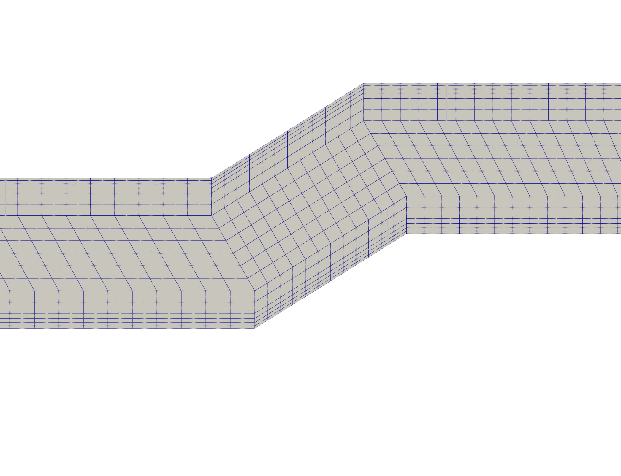
Figure 3: The boundary layers in the channel.

The mesh was created using Cubit and a stp file provided by the reactor designer. The file was exported to the Exodus format and converted to the Nek-supported .re2 using the utility exo2nek. If Nek5000/bin is added to the $PATH, exo2nek can be executed directly from the command line. The tool guides the user through the mesh conversion process. In this case, we recommend skipping the element right-handedness check for the mesh and proceeding with the mesh conversion process as suggested by the command line prompts.

Wall resolution can be verified by checking $var element = document.getElementById("moose-equation-872b23cf-94d4-44ef-9f1a-b2b54565dff3");katex.render("y+", element, {displayMode:false,throwOnError:false});$ values call the print_yplimits subroutine (provided in the extract_yp.f file) in userchk at whatever frequency is desired. The subroutine calculates $var element = document.getElementById("moose-equation-ddddac41-baff-4332-8c9f-72e2ef092537");katex.render("y+", element, {displayMode:false,throwOnError:false});$ values and outputs a variety of relevant metrics, the most important being the ratio of wall points with $var element = document.getElementById("moose-equation-3969d113-ee78-4699-b144-b171ee64cd37");katex.render("y+ \\leq 1", element, {displayMode:false,throwOnError:false});$ to the total number of wall points, outputted as ratio less than 1.0 is : in the logfile. Ideally, this ratio should be nearly 1.0. The $var element = document.getElementById("moose-equation-aa13b536-c6fe-464f-9195-4ad152fa521a");katex.render("y+", element, {displayMode:false,throwOnError:false});$ values can also be visualized using the output array from print_yplimits dumped into a Nek5000 output file using the outpost function.

Statistics at runtime and postprocessing

To iterate on the Reynolds number until the correct pressure drop of zero is obtained we need to calculate the pressure drop across the channel. We also need to calculate the Nusselt number, mean and outlet temperatures, and monitor a variety of other quantities for convergence. Our averaging code can monitor simulations as they run, using lines printed in the logfile. The basic idea behind our code is to construct masks or maps that identify the correct points or element faces based on coordinate ranges. We want to do this once, at the beginning of the simulation in usrdat2, to not have to waste computational time looking for the same elements at every time step (which is what would occur if the following code were placed in userchk instead of usrdat2). We create element maps/masks, that store local element and face IDs based on the element's centroid being between a certain coordinate range, and the face lying along a normal

c    element map of lower plane, close to inlet
      norm1  = (/0.0,1.0,0.0/)
      ptmin1 = (/-764.0,-1163.0,0.0/)
      ptmax1 = (/-723.0,-1157.0,0.0/)

      call emap_nsurf(emap_lo,exyzlo,norm1,ptmin1,ptmax1)
      call test_emap(emap_lo,'elo')

The above code will store zeros in the emap_lo array, indicating the local element ID corresponding to that index of emap_lo belongs to an element whose centroid does not lie in the specified range of x and y values. For elements that do lie within the specified coordinate range, the corresponding value of emap_lo at the index corresponding to the local element ID stores the face that has a normal closest to the normal specified. To verify the correct elements and faces have been selected, the test_emap function can be used. It will create a Nek output file with the name elo<casename>.nek5000, which can be opened in Paraview. Look at the x-velocity field - the element map emap_lo will be highlighted with values equal to 1.0 at each node on the face. The rest of the points will be zero.

Now that we have stored the element and face IDs that we need, we can average over faces using functions in the aravg.f file, that rely on Nek5000's internal functions facint_v and facint_a, which require element and face IDs as arguments. This will allow us to calculate area averages across the selected faces. Volumetric averages can be computed by constructing masks of nodes between a range of x and y values, using the following code

c     create masks for volumetric averages
      ptmin1 = (/-788.0,-1153.7,0.0/)
      ptmax1 = (/-720.0,1210.79,0.0/)
      call create_mask(msk_inout,ptmin1,ptmax1)

These element maps can be stored in a common block, so that they are accessible in userchk despite being created in usrdat2. To average any of the Nek5000 solution arrays over these element maps, simply call the following functions from aravg.f in userchk, such as

c     calculating averages of vx,vy,temp,k,tau

      uinav = emap_avg(vx,emap_in)
      vinav = emap_avg(vy,emap_in)
      tinav   = emap_avg(t(1,1,1,1,1),emap_in)
      kinav   = emap_avg(t(1,1,1,1,2),emap_in)
      tauinav = emap_avg(t(1,1,1,1,3),emap_in)

Bulk averages can be calculated similarly using the point masks and the bulkavg function. Weighted scalar averages or area integrals can be calculated using the emap_scalar_avg function. The variables can be saved, for example, using a common block, and the difference between their values at successive time-steps printed to monitor convergence. Gradients for calculating the Nusselt number are obtained using Nek5000's gradm1 subroutine, and the gradients are averaged over the hot-wall to obtain a heat flux using Nek5000's facint function.

Using these postprocessing functions, we can monitor the pressure drop across the channel at runtime by calculating the average pressure at the top and bottom of the channel, and iterating on the Reynolds number until the difference between the calculated pressure drop and the target pressure drop is below the solver tolerance.

c     pressure drop calculation
      pin = emap_avg(pr,emap_lo)
      pout = emap_avg(pr,emap_hi)
      dp = pin - pout

Input parameters

A list of miscellaneous input parameters is included in Table 1 for reproducibility.

Table 1: Simulation input parameters.

Parameter	Value	Unit
Inlet temperature	323.15	K
Hot wall temperature	693.15	K
Density	1.10342 (Lemmon et al., 2000)	kg m $var element = document.getElementById("moose-equation-e636d044-a200-4f76-b7ef-1a735c92fa3c");katex.render("^{-3}", element, {displayMode:false,throwOnError:false});$
Viscosity	1.951 $var element = document.getElementById("moose-equation-734f0c50-1b0e-4e9d-b61e-c27f368b4ef2");katex.render("\\times", element, {displayMode:false,throwOnError:false});$ 10 $var element = document.getElementById("moose-equation-d86dbbd5-80e0-41cc-a4ed-533cc173bb78");katex.render("^{-5}", element, {displayMode:false,throwOnError:false});$ (Kestin and Whitelaw, 1964)	Pa s
Thermal conductivity	0.02766 (Stephan and Laesecke, 1985)	W m $var element = document.getElementById("moose-equation-0be879a4-feee-49c4-8371-80f348da5dd4");katex.render("^{-1}", element, {displayMode:false,throwOnError:false});$ K $var element = document.getElementById("moose-equation-fe3e559b-17de-4254-af7e-9007ec5b9e67");katex.render("^{-1}", element, {displayMode:false,throwOnError:false});$
Specific Heat Capacity $var element = document.getElementById("moose-equation-fc4e011b-4a1c-4ccc-b4f9-e0023281d5e5");katex.render("c_p", element, {displayMode:false,throwOnError:false});$	1007.4333 (Lemmon et al., 2000)	J kg $var element = document.getElementById("moose-equation-4520c3bb-ff41-4654-bf6c-882b37f983ed");katex.render("^{-1}", element, {displayMode:false,throwOnError:false});$ K $var element = document.getElementById("moose-equation-1de979db-63ea-404a-ad18-21368ebf0f47");katex.render("^{-1}", element, {displayMode:false,throwOnError:false});$
Prandtl Number	0.710594	-
Characteristic length	40	mm
$var element = document.getElementById("moose-equation-4b9fc82c-2c0d-4aa9-8b54-b055b7bfbbfa");katex.render("T_0", element, {displayMode:false,throwOnError:false});$ (Eq. (5))	323.15	K
$var element = document.getElementById("moose-equation-9a7964ad-58f5-4e7c-b1a3-226a610cf16f");katex.render("\\Delta T", element, {displayMode:false,throwOnError:false});$ (Eq. (5))	370.0	K
Pressure solver tolerance	10 $var element = document.getElementById("moose-equation-dcddd4a0-4add-42a6-aa09-5571cf0f7b28");katex.render("^{-4}", element, {displayMode:false,throwOnError:false});$	-
Velocity solver tolerance	10 $var element = document.getElementById("moose-equation-ee6fcd5b-a5d7-4f03-ae48-9a53a3e9b027");katex.render("^{-6}", element, {displayMode:false,throwOnError:false});$	-
$var element = document.getElementById("moose-equation-c07ad7cd-9931-4494-b04b-ecd9ad81b671");katex.render("k", element, {displayMode:false,throwOnError:false});$ solver tolerance	10 $var element = document.getElementById("moose-equation-03ecaebc-5e01-4c80-bcd3-bc40441d90f7");katex.render("^{-8}", element, {displayMode:false,throwOnError:false});$	-
$var element = document.getElementById("moose-equation-50db9c2b-d202-43cd-b265-c8889583d15e");katex.render("\\tau", element, {displayMode:false,throwOnError:false});$ solver tolerance	10 $var element = document.getElementById("moose-equation-1eb0de6f-f45d-4df7-b800-8cc9755811d8");katex.render("^{-6}", element, {displayMode:false,throwOnError:false});$	-

Results

The velocity and temperature results obtained are shown in Figure 4 and Figure 5. The flow enters the domain from the bottom left in the lower plenum, and accelerates in the hot channel due to a narrowing of the cross-section and due to the Boussinesq acceleration term. The air leaves the heated channel and enters the upper plenum in a state biased entirely towards the top of the plenum. The gradual ramping down of the Boussinesq term in the upper plenum gradually redistributes this jet and allows it to exit the domain without any backflow at the outlet, while causing no impact on the results upstream. The relatively low Reynolds number in the hot channel (obtained both through correlations and our iterative analysis) does not promote significant mixing in the channel itself. For the purposes of visualization, the excess upper plenum outlet region has been clipped by about 50% to remove the region that exists only for allowing the flow to redistribute and exit the domain cleanly.

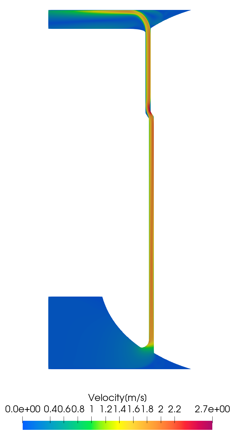
Figure 4: The velocity solution.

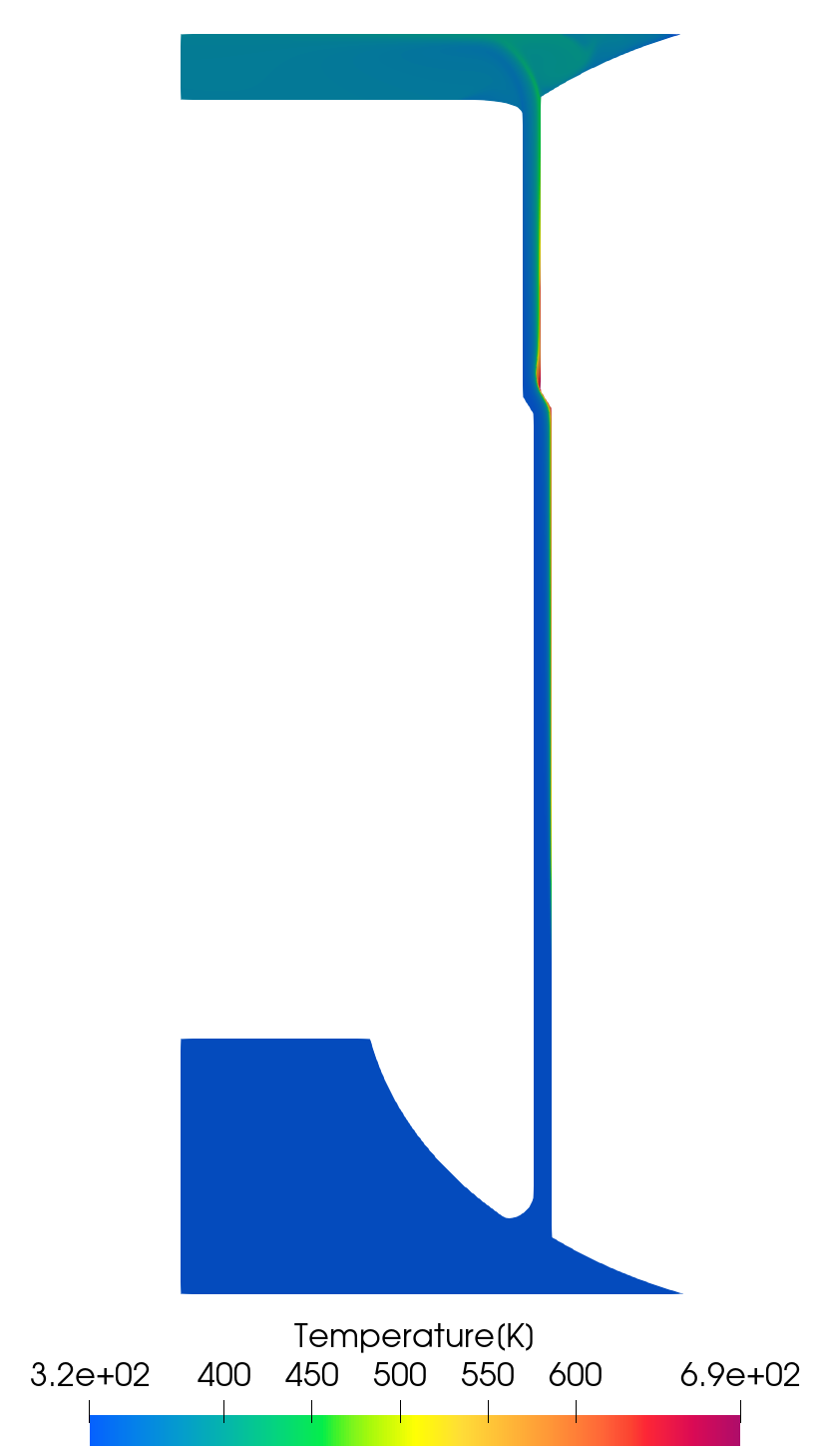
Figure 5: The temperature solution.

The quantities of interest calculated from steady state results are summarized in Table 2. Note that CFD also allows the estimation of certain data that cannot be reliably estimated from correlations alone without significant approximations and simplifications.

Table 2: Summary of results.

Parameter	Correlation-based estimate	CFD-based result	Units
Reynolds Number	3152.99	3580	-
Friction Factor	0.0409	0.028403	-
Nusselt Number	13.98	13.53	-
Bulk temperature	-	352.458	K
Outlet temperature	-	383.394	K
Heat flux	-	3.01 $var element = document.getElementById("moose-equation-7d88848b-4f42-4611-b55e-472a6a5fd69c");katex.render("\\times", element, {displayMode:false,throwOnError:false});$ 10 $var element = document.getElementById("moose-equation-b37ce46a-d699-4269-b89a-88c1b41db503");katex.render("^3", element, {displayMode:false,throwOnError:false});$	W m $var element = document.getElementById("moose-equation-08a99582-3914-4820-aa71-159d8db69b29");katex.render("^{-2}", element, {displayMode:false,throwOnError:false});$
Heat removed per second	-	2.072 $var element = document.getElementById("moose-equation-f847f60f-bf5d-460e-993e-72f22e84a61e");katex.render("\\times", element, {displayMode:false,throwOnError:false});$ 10 $var element = document.getElementById("moose-equation-9b465fcb-1f82-4d81-b5e9-085095f20991");katex.render("^4", element, {displayMode:false,throwOnError:false});$	W

Run Command

To generate an .ma2 file for your mesh (.re2), use genmap, as described in the Nek5000 tutorial. Adjust the mesh resolution and other parameters in the SIZE file, and compile using makenek <casename>. To run the case, execute


nekbmpi airjacket 144

which uses the script nekbmpi to internally call mpiexec. On some HPC systems, srun may be required instead.

References

ANL. Nek5000 Version 19.0. Argonne National Laboratory, Illinois, 2019. URL: https://nek5000.mcs.anl.gov.

@article{anl_nek5000_2019,
    author = "ANL",
    title = "Nek5000 {Version} 19.0",
    url = "https://nek5000.mcs.anl.gov",
    journal = "Argonne National Laboratory, Illinois",
    year = "2019"
}

M. O. Deville, P. F. Fischer, and E. H. Mund. High-Order Methods for Incompressible Fluid Flow. Cambridge Monographs on Applied and Computational Mathematics, August 2002. URL: /core/books/highorder-methods-for-incompressible-fluid-flow/D59381B3A2968E7ADED018C47201964C (visited on 2019-10-29), doi:10.1017/CBO9780511546792.

@book{deville_high-order_2002,
    author = "Deville, M. O. and Fischer, P. F. and Mund, E. H.",
    title = "High-{Order} {Methods} for {Incompressible} {Fluid} {Flow}",
    url = "/core/books/highorder-methods-for-incompressible-fluid-flow/D59381B3A2968E7ADED018C47201964C",
    urldate = "2019-10-29",
    publisher = "Cambridge Monographs on Applied and Computational Mathematics",
    month = "August",
    year = "2002",
    doi = "10.1017/CBO9780511546792"
}

Paul F. Fischer and Ananias G. Tomboulides. Chapter 3 - Spectral element methods for turbulence. In Robert D. Moser, editor, Numerical Methods in Turbulence Simulation, Numerical Methods in Turbulence, pages 95–137. Academic Press, January 2023. URL: https://www.sciencedirect.com/science/article/pii/B9780323911443000097 (visited on 2023-08-09), doi:10.1016/B978-0-32-391144-3.00009-7.

@incollection{fischer_chapter_2023,
    author = "Fischer, Paul F. and Tomboulides, Ananias G.",
    editor = "Moser, Robert D.",
    series = "Numerical {Methods} in {Turbulence}",
    title = "Chapter 3 - {Spectral} element methods for turbulence",
    isbn = "978-0-323-91144-3",
    url = "https://www.sciencedirect.com/science/article/pii/B9780323911443000097",
    language = "en",
    urldate = "2023-08-09",
    booktitle = "Numerical {Methods} in {Turbulence} {Simulation}",
    publisher = "Academic Press",
    month = "January",
    year = "2023",
    doi = "10.1016/B978-0-32-391144-3.00009-7",
    keywords = "High-order finite elements, Iterative solvers, Operator splitting, Spectral element methods, Turbulence, Unstructured domains",
    pages = "95--137"
}

K. J. Hsieh and F. S. Lien. Numerical modeling of buoyancy-driven turbulent flows in enclosures. International Journal of Heat and Fluid Flow, 25(4):659–670, August 2004. URL: https://www.sciencedirect.com/science/article/pii/S0142727X03001565 (visited on 2023-05-01), doi:10.1016/j.ijheatfluidflow.2003.11.023.

@article{hsieh_numerical_2004,
    author = "Hsieh, K. J. and Lien, F. S.",
    title = "Numerical modeling of buoyancy-driven turbulent flows in enclosures",
    volume = "25",
    issn = "0142-727X",
    url = "https://www.sciencedirect.com/science/article/pii/S0142727X03001565",
    doi = "10.1016/j.ijheatfluidflow.2003.11.023",
    language = "en",
    number = "4",
    urldate = "2023-05-01",
    journal = "International Journal of Heat and Fluid Flow",
    month = "August",
    year = "2004",
    keywords = "Natural convection, Non-linear – model, Unsteady RANS",
    pages = "659--670"
}

Frank E. Jones. The Air Density Equation and the Transfer of the Mass Unit. Journal of Research of the National Bureau of Standards, 83(5):419–428, 1978. URL: https://www.ncbi.nlm.nih.gov/pmc/articles/PMC6764509/ (visited on 2023-08-10), doi:10.6028/jres.083.028.

@article{jones_air_1978,
    author = "Jones, Frank E.",
    title = "The {Air} {Density} {Equation} and the {Transfer} of the {Mass} {Unit}",
    volume = "83",
    issn = "0160-1741",
    url = "https://www.ncbi.nlm.nih.gov/pmc/articles/PMC6764509/",
    doi = "10.6028/jres.083.028",
    number = "5",
    urldate = "2023-08-10",
    journal = "Journal of Research of the National Bureau of Standards",
    year = "1978",
    pmid = "34565996",
    pmcid = "PMC6764509",
    pages = "419--428"
}

J. Kestin and J. H. Whitelaw. The viscosity of dry and humid air. International Journal of Heat and Mass Transfer, 7(11):1245–1255, November 1964. URL: https://www.sciencedirect.com/science/article/pii/0017931064900663 (visited on 2023-08-10), doi:10.1016/0017-9310(64)90066-3.

@article{kestin_viscosity_1964,
    author = "Kestin, J. and Whitelaw, J. H.",
    title = "The viscosity of dry and humid air",
    volume = "7",
    issn = "0017-9310",
    url = "https://www.sciencedirect.com/science/article/pii/0017931064900663",
    doi = "10.1016/0017-9310(64)90066-3",
    language = "en",
    number = "11",
    urldate = "2023-08-10",
    journal = "International Journal of Heat and Mass Transfer",
    month = "November",
    year = "1964",
    pages = "1245--1255"
}

J. C. Kok and S. P. Spekreijse. Efficient and accurate implementation of the k-omega turbulence model in the NLR multi-block Navier-Stokes system. Technical Report, Nationaal Lucht- en Ruimtevaartlaboratorium, 2000. URL: https://reports.nlr.nl/handle/10921/822 (visited on 2021-04-21).

@TechReport{kok_efficient_2000,
    author = "Kok, J. C. and Spekreijse, S. P.",
    title = "Efficient and accurate implementation of the k-omega turbulence model in the {NLR} multi-block {Navier}-{Stokes} system",
    url = "https://reports.nlr.nl/handle/10921/822",
    institution = "Nationaal Lucht- en Ruimtevaartlaboratorium",
    urldate = "2021-04-21",
    year = "2000"
}

Eric W. Lemmon, Richard T Jacobsen, Steven G. Penoncello, and Daniel G. Friend. Thermodynamic Properties of Air and Mixtures of Nitrogen, Argon, and Oxygen From 60 to 2000 K at Pressures to 2000 MPa. Journal of Physical and Chemical Reference Data, 29(3):331–385, May 2000. URL: https://doi.org/10.1063/1.1285884 (visited on 2023-08-09), doi:10.1063/1.1285884.

@article{lemmon_thermodynamic_2000,
    author = "Lemmon, Eric W. and Jacobsen, Richard T and Penoncello, Steven G. and Friend, Daniel G.",
    title = "Thermodynamic {Properties} of {Air} and {Mixtures} of {Nitrogen}, {Argon}, and {Oxygen} {From} 60 to 2000 {K} at {Pressures} to 2000 {MPa}",
    volume = "29",
    issn = "0047-2689",
    url = "https://doi.org/10.1063/1.1285884",
    doi = "10.1063/1.1285884",
    number = "3",
    urldate = "2023-08-09",
    journal = "Journal of Physical and Chemical Reference Data",
    month = "May",
    year = "2000",
    pages = "331--385"
}

K. Stephan and A. Laesecke. The Thermal Conductivity of Fluid Air. Journal of Physical and Chemical Reference Data, 14(1):227–234, January 1985. URL: https://doi.org/10.1063/1.555749 (visited on 2023-08-09), doi:10.1063/1.555749.

@article{stephan_thermal_1985,
    author = "Stephan, K. and Laesecke, A.",
    title = "The {Thermal} {Conductivity} of {Fluid} {Air}",
    volume = "14",
    issn = "0047-2689",
    url = "https://doi.org/10.1063/1.555749",
    doi = "10.1063/1.555749",
    number = "1",
    urldate = "2023-08-09",
    journal = "Journal of Physical and Chemical Reference Data",
    month = "January",
    year = "1985",
    pages = "227--234"
}

(microreactors/gcmr/airjacket/re_estimate.py)

import scipy as scp
import numpy as np
import matplotlib.pyplot as plt

turbulent = 1# 0 implies laminar, >0 implies turbulent

#=======================================
# full mesh, 2D
#=======================================
H = 2.36368 #from channel base to top
Dh = 40./1000.
Aw = 30727.523993417268/1000.0/1000.0 # cross-section area of the channel
Ahot = 1095958.0485001195/1000.0/1000.0 #area of the hot wall

#material properties, temperature BCs

rho_amb = 1.103236458 # ambient density at 50 deg C
kelvin = 273.15
T_in = 50.0 + kelvin
T_hot = (420.0 + kelvin) #*0.6337 # sinusoid, can also comment out 0.6 for constant BC
mu = 0.00001951
M_air = 28.9647/1000.0 # kg/mol
k_fluid = 0.02766 #W/m/K
P_atm = 101325.0
Cp = 1007.433186
Rgc = 8.314 # gas constant
g = 9.80665
Pr = mu*Cp/k_fluid
beta = 1.0/T_in

#=======================================

def T_mean(tout):
    return 0.5*(tout+T_in)

def rho_mean(to):
    return P_atm*M_air/Rgc/T_mean(to)

def reno(ub):
    return rho_amb*ub*Dh/mu

def fdturb(ub):
    return 0.3164*(reno(ub))**(-0.25) #Blasius, turbulent friction factor

def fdlam(ub):
    return 64.0/reno(ub)

def htcoeff(ub):
    return (k_fluid/Dh)*(0.023 * (reno(ub)**(0.8)) * Pr**(0.4)) #Dittus-Boelter, turbulent

def htlam():
    return (k_fluid/Dh)*(3.66) #Incropera, laminar

def pqbalance_lam(ubto):
    ub, to = ubto
    expr1 = (rho_amb*beta*(T_mean(to)-T_in)*g*H) - (fdlam(ub)*rho_amb*ub*ub*H/2.0/Dh)  # P balance
    expr2 = (Ahot*htlam()*(T_hot-T_mean(to))) - (rho_amb*ub*Aw*Cp*(to-T_in))      # q balance
    return (expr1,expr2)

def richardson(ub):
    return g*beta*(T_hot-T_in)*Dh/ub/ub

def pqbalance(ubto):
    ub, to = ubto
    #turbulent:
    expr1 = (rho_amb*beta*(T_mean(to)-T_in)*g*H) - (fdturb(ub)*rho_amb*ub*ub*H/2.0/Dh)
    expr2 = (Ahot*htcoeff(ub)*(T_hot-T_mean(to))) - (rho_amb*ub*Aw*Cp*(to-T_in))

    return (expr1,expr2)

if (turbulent):
    #turbulent solve
    Ubar, Tout =  scp.optimize.fsolve(pqbalance, (1.0, 0.5*(T_hot+T_in)))
else:
    # laminar solve
    Ubar, Tout =  scp.optimize.fsolve(pqbalance_lam, (0.5, 0.5*(T_hot+T_in)))

print("Mean velocity, outlet temp:",Ubar," m/s ", Tout, " K")

if (turbulent):
    # print residuals for balance equations assuming turbulent flow:
    print("Residual of turbulent momentum, energy balance:",pqbalance((Ubar,Tout)))
else:
    # print residuals for balance equations assuming laminar flow:
    print("Residual of laminar momentum, energy balance:",pqbalance_lam((Ubar,Tout)))


print("Reynolds no.:",reno(Ubar))
print("Friction factor:",fdturb(Ubar))
print("Mean density:",rho_mean(Tout))
print("Bulk temperature:",T_mean(Tout))
print("Richardson number:",richardson(Ubar))

(microreactors/gcmr/airjacket/airjacket.usr)

c #include "experimental/rans_komg.f"

      include "rans_komg.f"
      include "extract_yp.f"
      include "aravg.f"
      include "limits.f"
      include "recycle.f"
      include "utilities.f"
c-----------------------------------------------------------------------
c  nek5000 user-file template
c
c  user specified routines:
c     - uservp  : variable properties
c     - userf   : local acceleration term for fluid
c     - userq   : local source term for scalars
c     - userbc  : boundary conditions
c     - useric  : initial conditions
c     - userchk : general purpose routine for checking errors etc.
c     - usrdat  : modify element vertices 
c     - usrdat2 : modify mesh coordinates
c     - usrdat3 : general purpose routine for initialization
c     
c-----------------------------------------------------------------------
      subroutine uservp(ix,iy,iz,eg) ! set variable properties
      implicit none
      include 'SIZE'
      include 'TOTAL'
      include 'NEKUSE'

      integer ix,iy,iz,e,eg
      real rans_mut,rans_mutsk,rans_mutso,rans_turbPrandtl
      real mu_t,Pr_t

      e = gllel(eg)

      Pr_t=rans_turbPrandtl()
      mu_t=rans_mut(ix,iy,iz,e)

      if(ifield.eq.1) then
        t(ix,iy,iz,e,4)=mu_t/cpfld(ifield,1) !store eddy viscosity for post processing
        udiff = cpfld(ifield,1)+mu_t
        utrans = cpfld(ifield,2)
      elseif(ifield.eq.2) then
        udiff = cpfld(ifield,1)+mu_t*cpfld(ifield,2)/(Pr_t*cpfld(1,2))
        utrans = cpfld(ifield,2)
      elseif(ifield.eq.3) then !use rho and mu from field 1
        udiff = cpfld(1,1)+rans_mutsk(ix,iy,iz,e)
        utrans = cpfld(1,2)
      elseif(ifield.eq.4) then !use rho and mu from field 1
        udiff = cpfld(1,1)+rans_mutso(ix,iy,iz,e)
        utrans = cpfld(1,2)
      endif

      return
      end
c-----------------------------------------------------------------------
      subroutine userf(ix,iy,iz,eg) ! set acceleration term
      implicit none
      include 'SIZE'
      include 'TOTAL'
      include 'NEKUSE'
c
c     Note: this is an acceleration term, NOT a force!
c     Thus, ffx will subsequently be multiplied by rho(x,t).
c     userf is only called for velocity
c     temp is preloaded with t(ix,iy,iz,ie,1): see bdry.f:1181

      real Ri
      common /boussinesq/ Ri

      integer ix,iy,iz,eg,e
      real ybnd1,ybnd2, xx, yy, mb, cb,temp_mosdef

      real xmin,xmax,ymin,ymax,zmin,zmax
      common /dmn_size/ xmin,xmax,ymin,ymax,zmin,zmax

      ybnd1 = 0.6*ymax
      ybnd2 = 0.8*ymax
      mb = -1.0/(ybnd2-ybnd1)
      cb = -ybnd2*mb

      e = gllel(eg)
      xx = xm1(ix,iy,iz,e)
      yy = ym1(ix,iy,iz,e)

      ffz = 0.0
      ffy = 0.0
      ffx = Ri*temp
      if(yy.gt.ybnd1.and.yy.le.ybnd2.and.xx.gt.0.0) then ! ramping down gradually
        ffx = (mb*yy+cb)*Ri*temp
      endif
      if(yy.gt.ybnd2.and.xx.gt.0.0) then
        ffx = 0.0
      endif

      return
      end
c-----------------------------------------------------------------------
      subroutine userq(ix,iy,iz,eg) ! set source term
      implicit none
      include 'SIZE'
      include 'TOTAL'
      include 'NEKUSE'

      integer ix,iy,iz,e,eg
      real rans_kSrc,rans_omgSrc
      real rans_kDiag,rans_omgDiag

      e = gllel(eg)

      if(ifield.eq.3) then
        qvol = rans_kSrc(ix,iy,iz,e)
        avol = rans_kDiag(ix,iy,iz,e)
      elseif(ifield.eq.4) then
        qvol = rans_omgSrc(ix,iy,iz,e)
        avol = rans_omgDiag(ix,iy,iz,e)
      else
        qvol = 0.0
      endif

      return
      end
c-----------------------------------------------------------------------
      subroutine userbc(ix,iy,iz,iside,eg) ! set up boundary conditions
      implicit none
      include 'SIZE'
      include 'TOTAL'
      include 'NEKUSE'
c
c     NOTE ::: This subroutine MAY NOT be called by every process
c
      integer ix,iy,iz,iside,e,eg
    
C     U, TKE, and Omg are all zero on the wall 

      real xbnd1,xbnd2,xx,xhat,mx,cx

      real Re,mu0,rho0,Uc,T0,cp0,k0,Lc,L0,Thw
      common /props/ Re,mu0,rho0,Uc,T0,cp0,k0,Lc,L0,Thw

      e = gllel(eg)

      ux = 0.0 
      uy = -3.5630245817969738E-002 
      temp = 0.0

      if(cbc(iside,e,1).eq.'W  ') then           ! walls
        if(ifield.eq.3) temp = 0.0
        if(ifield.eq.4) temp = 0.0
      endif

      if(boundaryID(iside,e).eq.1) then           ! inlet
        if(ifield.eq.3) temp = 0.01! kibc(ix,iy,iz,e)
        if(ifield.eq.4) temp = 0.2 ! tauibc(ix,iy,iz,e)
      endif

      xbnd1 = -675.0/Lc
      xbnd2 = 824.9764/Lc
      xbnd2 = 0.1*(xbnd2-xbnd1) + xbnd1
      mx = 1.0/(xbnd2-xbnd1)
      cx = 1.0 - mx*xbnd2

      if(boundaryID(iside,e).eq.3.and.ifield.eq.2) then           ! hot wall
       xx = xm1(ix,iy,iz,e)
       if(xx.le.xbnd2) then       
        temp = mx*xx + cx
       else
        temp = 1.0
       endif
      endif

      return
      end
c-----------------------------------------------------------------------
      subroutine useric(ix,iy,iz,eg) ! set up initial conditions
      implicit none
      include 'SIZE'
      include 'TOTAL'
      include 'NEKUSE'

      integer ix,iy,iz,e,eg
      real xx,xtop

      real Re,mu0,rho0,Uc,T0,cp0,k0,Lc,L0,Thw
      common /props/ Re,mu0,rho0,Uc,T0,cp0,k0,Lc,L0,Thw

      e = gllel(eg)
      xx = xm1(ix,iy,iz,e)
      xtop = 30.0

      ux   = 0.0001
      uy   = -0.0001
      if (xx.gt.xtop) uy = 0.0001
      uz   = 0.0
      temp = 0.0

      if(ifield.eq.3) temp = 0.01 !97662386491144943E-005
      if(ifield.eq.4) temp = 0.2  !6.8956997219801952

      return
      end
c-----------------------------------------------------------------------
      subroutine userchk()
      implicit none
      include 'SIZE'
      include 'TOTAL'
      include 'NEKUSE'

      integer ntot,e,f,i
      real ypout(lx1,ly1,lz1,lelt),wd(lx1,ly1,lz1,lelt)

      real uinav,vinav,tinav,kinav,tauinav,
     $  uhwav,vhwav,thwav,khwav,tauhwav,
     $  ucwav,vcwav,tcwav,kcwav,taucwav,
     $  uloav,vloav,tloav,kloav,tauloav,
     $  umiav,vmiav,tmiav,kmiav,taumiav,
     $  uhiav,vhiav,thiav,khiav,tauhiav

      real Ri
      common /boussinesq/ Ri

      real dp1, dp2, tm1, tm2, qav1, qav2
      common /residuals/ dp1, dp2, tm1, tm2, qav1, qav2

      real g,Tm
      real ones(lx1,ly1,lz1,lelv)
      real pin,pout,dp
      real nu,gradt_av,areahw,thw_ndim,Tb,qav,qin,qout
      real xx,yy,zz,xhw_lo,xhw_hi
      real dtx(lx1,ly1,lz1,lelv),dty(lx1,ly1,lz1,lelv),
     $ dtz(lx1,ly1,lz1,lelv)
      real tdim(lx1,ly1,lz1,lelt)

      real bulkavg, emap_avg, facint, glsum,
     $             emap_area,planar_ave_m1,emap_scalar_avg

      real fluxw(lx1,ly1,lz1,lelt)
      real fluxv(lx1,ly1,lz1,lelt)
      real fluxo(lx1,ly1,lz1,lelt)

      integer ierr
      real fmin,fmax,fmean
      real glmin,glmax,surf_integral

      real Re,mu0,rho0,Uc,T0,cp0,k0,Lc,L0,Thw
      common /props/ Re,mu0,rho0,Uc,T0,cp0,k0,Lc,L0,Thw

      integer  emap_lo(lelv),emap_cw(lelv),emap_in(lelv),
     $      emap_hi(lelv), emap_mi(lelv),emap_hw(lelv)
      real exyzlo(3), exyzhi(3), exyzmi(3)

      common /roi/ emap_lo,emap_cw,emap_in,emap_hi,
     $         emap_mi,emap_hw, exyzlo, exyzhi, exyzmi

      real msk_inout(lx1,ly1,lz1,lelv),msk_hw(lx1,ly1,lz1,lelv)
      common /masks/ msk_inout,msk_hw

      real xmin,xmax,ymin,ymax,zmin,zmax
      common /dmn_size/ xmin,xmax,ymin,ymax,zmin,zmax

      integer iglsum

c     if your new mesh differs significantly from the previous one
c     you can use gfldr to provide an initial condition using an 
c     output file based off of the old mesh

c      if (istep.eq.0) call gfldr('restart2.fld')

      ntot = lx1*ly1*lz1*nelt

c     calculating mean temperature, Richardson number - affects flow!
      call rone(ones,ntot)
      Tm = bulkavg(t(1,1,1,1,1),ones,msk_inout)
      Tm = (Tm*(Thw-T0)) + T0
      g = 9.8
      Ri = g * (1.0/T0)*(Thw-T0)*(Lc/1000.0)/Uc/Uc

c     The code below is entirely for post-processing

c     calculating averages of vx,vy,temp,k,tau

      uinav = emap_avg(vx,emap_in)
      vinav = emap_avg(vy,emap_in)
      tinav   = emap_avg(t(1,1,1,1,1),emap_in)
      kinav   = emap_avg(t(1,1,1,1,2),emap_in)
      tauinav = emap_avg(t(1,1,1,1,3),emap_in)

      uhwav = emap_avg(vx,emap_hw)
      vhwav = emap_avg(vy,emap_hw)
      thwav   = emap_avg(t(1,1,1,1,1),emap_hw)
      khwav   = emap_avg(t(1,1,1,1,2),emap_hw)
      tauhwav = emap_avg(t(1,1,1,1,3),emap_hw)

      ucwav = emap_avg(vx,emap_cw)
      vcwav = emap_avg(vy,emap_cw)
      tcwav   = emap_avg(t(1,1,1,1,1),emap_cw)
      kcwav   = emap_avg(t(1,1,1,1,2),emap_cw)
      taucwav = emap_avg(t(1,1,1,1,3),emap_cw)

      uloav = emap_avg(vx,emap_lo)
      vloav = emap_avg(vy,emap_lo)
      tloav   = emap_avg(t(1,1,1,1,1),emap_lo)
      kloav   = emap_avg(t(1,1,1,1,2),emap_lo)
      tauloav = emap_avg(t(1,1,1,1,3),emap_lo)

      umiav = emap_avg(vx,emap_mi)
      vmiav = emap_avg(vy,emap_mi)
      tmiav   = emap_avg(t(1,1,1,1,1),emap_mi)
      kmiav   = emap_avg(t(1,1,1,1,2),emap_mi)
      taumiav = emap_avg(t(1,1,1,1,3),emap_mi)

      uhiav = emap_avg(vx,emap_hi)
      vhiav = emap_avg(vy,emap_hi)
      thiav   = emap_avg(t(1,1,1,1,1),emap_hi)
      khiav   = emap_avg(t(1,1,1,1,2),emap_hi)
      tauhiav = emap_avg(t(1,1,1,1,3),emap_hi)

c     pressure drop calculation
      pin = emap_avg(pr,emap_lo)
      pout = emap_avg(pr,emap_hi)
      dp = pin - pout

c     heat flux calculation
      call gradm1(dtx,dty,dtz,t)

      gradt_av = 0.0

      do e=1,nelt
       do f=1,ndim*2
        if (boundaryID(f,e).eq.3) then
          gradt_av = gradt_av + facint(dtx,unx,area,f,e) +
     $              facint(dty,uny,area,f,e)
        endif
       enddo
      enddo

      gradt_av = glsum(gradt_av,1)
      areahw = emap_area(emap_hw)
      gradt_av = gradt_av/areahw

      thw_ndim = emap_avg(t,emap_hw)
      Tb = bulkavg(t,vx,msk_inout)
      nu = gradt_av/(thw_ndim-Tb)
      qav = gradt_av

      qin = emap_scalar_avg(t,vx,emap_lo,0)
      qin = qin + (gradt_av*areahw*cpfld(2,1))

      qout = emap_scalar_avg(t,vx,emap_hi,0)

      if (istep.eq.0) then
        dp2 = 0.
        tm2 = 0.
        qav2 = 0.
      endif

      dp1 = dp2
      dp2 = dp
      tm1 = tm2
      tm2 = Tm
      qav1 = qav2
      qav2 = qav

      if (nio.eq.0) then
       write(6,81) uinav,vinav,tinav,kinav,tauinav
       write(6,82) uhwav,vhwav,thwav,khwav,tauhwav
       write(6,83) ucwav,vcwav,tcwav,kcwav,taucwav
       write(6,84) uloav,vloav,tloav,kloav,tauloav
       write(6,85) umiav,vmiav,tmiav,kmiav,taumiav
       write(6,86) uhiav,vhiav,thiav,khiav,tauhiav

       write(6,87) dp,Tm,(dp2-dp1),(tm2-tm1)
       write(6,88) nu,qav,qin,qout,(qav2-qav1)
       write(6,89) Ri,Tm,areahw
      endif

c     prints y+ related info
      call print_yplimits(ypout,wd,1)

c     dumps y+ in the `x-velocity` field of yplairjacket.nek5000
c      call outpost(ypout,vy,vz,pr,t,'ypl')

81    format(1p5e16.8,': Inlet avg vx/vy/t/k/tau')
82    format(1p5e16.8,': HW avg vx/vy/t/k/tau')
83    format(1p5e16.8,': CW avg vx/vy/t/k/tau')
84    format(1p5e16.8,': Low avg vx/vy/t/k/tau')
85    format(1p5e16.8,': Mid avg vx/vy/t/k/tau')
86    format(1p5e16.8,': High avg vx/vy/t/k/tau')
87    format(1p4e16.8,': dP,Tm, res_dp,res_Tm')
88    format(1p5e16.8,': Nusselt no./avg heat flux[W/sq m]/'
     $                   'q in[-]/q out[-]/dq_av diff')
89    format(1p3e16.8,': Richardson number, mean temp[K],areahw')

      return
      end
c-----------------------------------------------------------------------
      subroutine usrdat()   ! This routine to modify element vertices
      implicit none
      include 'SIZE'
      include 'TOTAL'


      return
      end
c-----------------------------------------------------------------------
      subroutine usrdat2()  ! This routine to modify mesh coordinates
      implicit none
      include 'SIZE'
      include 'TOTAL'

      real wd
      common /walldist/ wd(lx1,ly1,lz1,lelv)

      integer n,iel,ifc,id_face

      integer ifld_k,ifld_t,m_id,w_id
      real coeffs(30) !array for passing custom coeffs to RANS model
      logical ifcoeffs !flag to use custom or default coeffs

      real Re,mu0,rho0,Uc,T0,cp0,k0,Lc,L0,Thw
      common /props/ Re,mu0,rho0,Uc,T0,cp0,k0,Lc,L0,Thw

      integer  emap_lo(lelv),emap_cw(lelv),emap_in(lelv),
     $      emap_hi(lelv), emap_mi(lelv),emap_hw(lelv)
      real exyzlo(3), exyzhi(3), exyzmi(3)

      common /roi/ emap_lo,emap_cw,emap_in,emap_hi,
     $         emap_mi,emap_hw, exyzlo, exyzhi, exyzmi

      real msk_inout(lx1,ly1,lz1,lelv),msk_hw(lx1,ly1,lz1,lelv)
      common /masks/ msk_inout,msk_hw
      real xmin,xmax,ymin,ymax,zmin,zmax

      integer e,f,i
      real ptmin1(3),ptmin2(3),ptmin3(3),ptmin4(3),ptmin5(3)
      real ptmax1(3),ptmax2(3),ptmax3(3),ptmax4(3),ptmax5(3)
      real norm1(3),norm2(3),norm3(3)

      real calc_dh,emap_area
      real area_hw, area_hi, area_in
      real xx, yy, theta

      n=nx1*ny1*nz1*nelv

c     build element/face maps for postproc

      call emap_sideset(emap_in,1,1)
      call test_emap(emap_in,'ein')

      call emap_sideset(emap_hw,3,3)
      call test_emap(emap_hw,'ehw')

      call emap_sideset(emap_cw,4,4)
      call test_emap(emap_cw,'ecw')

c    element map of lower plane, close to inlet
      norm1  = (/0.0,1.0,0.0/)
      ptmin1 = (/-764.0,-1163.0,0.0/)
      ptmax1 = (/-723.0,-1157.0,0.0/)

      call emap_nsurf(emap_lo,exyzlo,norm1,ptmin1,ptmax1)
      call test_emap(emap_lo,'elo')

c    element map of upper plane, close to inlet
      norm2  = (/0.0,1.0,0.0/)
      ptmin2 = (/-788.2,1205.0,0.0/)
      ptmax2 = (/-748.2,1210.8,0.0/)

      call emap_nsurf(emap_hi,exyzhi,norm2,ptmin2,ptmax2)
      call test_emap(emap_hi,'ehi')

c    element map of upper plane, close to inlet
      norm3  = (/0.0,1.0,0.0/)
      ptmin3 = (/-789.0,813.0,0.0/)
      ptmax3 = (/-747.0,819.0,0.0/)

      call emap_nsurf(emap_mi,exyzmi,norm3,ptmin3,ptmax3)
      call test_emap(emap_mi,'emi')

      call set_initial_properties()

c     create masks for volumetric averages
      ptmin1 = (/-788.0,-1153.7,0.0/)
      ptmax1 = (/-720.0,1210.79,0.0/)
      call create_mask(msk_inout,ptmin1,ptmax1)

      call domain_size(xmin,xmax,ymin,ymax,zmin,zmax)
      ptmin2(1) = xmin
      ptmax2(1) = xmax
      ptmin2(2) = ptmin1(2)
      ptmax2(2) = ptmax1(2)
      call create_mask(msk_hw,ptmin2,ptmax2)

      call outpost(msk_inout,vy,vz,pr,t,'mio')
      call outpost(msk_hw,vy,vz,pr,t,'mhw')

C     rescale the domain BEFORE calling rans_init

      theta = pi/2.0
      do i=1,n
        xx = xm1(i,1,1,1)
        yy = ym1(i,1,1,1)
        xm1(i,1,1,1) =  xx*cos(theta) + yy*sin(theta)
        ym1(i,1,1,1) = -xx*sin(theta) + yy*cos(theta)
      enddo

      call outpost(vx,vy,vz,pr,t,'rot')
      call cmult(xm1,1.0/Lc,n)
      call cmult(ym1,1.0/Lc,n)


c     assign BCs to sidesets using cbc array
c      do e=1,nelv
c      do f=1,2*ndim
c        id_face = boundaryID(f,e)
c        if (id_face.eq.1) then        ! dirichlet (inlet)  BCs
c           cbc(f,e,1) = 'v  '
c           cbc(f,e,2) = 't  '
c        elseif (id_face.eq.2) then    ! Outlet
c           cbc(f,e,1) = 'O  '
c           cbc(f,e,2) = 'O  '
c        elseif (id_face.eq.3) then    ! Hot wall
c           cbc(f,e,1) = 'W  '
c           cbc(f,e,2) = 't  '
c        elseif (id_face.eq.4) then    ! Insulated wall
c           cbc(f,e,1) = 'W  '
c           cbc(f,e,2) = 'I  '
c        endif
c      enddo
c      enddo

C     Setup RANS model, this MUST be done in usrdat2

      ifld_k = 3         !field number for tke, t(1,1,1,1,ifld_k-1)
      ifld_t = 4         !field number for omega/tau, t(1,1,1,1,ifld_t-1)
      ifcoeffs = .false. !set to true to pass custom coefficients
      m_id = 4 !standard k-tau
      w_id = 2 ! distf (coordinate difference, provides smoother function)
      call rans_init(ifld_k,ifld_t,ifcoeffs,coeffs,w_id,wd,m_id)

      return
      end
c-----------------------------------------------------------------------
      subroutine usrdat3()
      implicit none
      include 'SIZE'
      include 'TOTAL'

      real xmin,xmax,ymin,ymax,zmin,zmax
      common /dmn_size/ xmin,xmax,ymin,ymax,zmin,zmax

      call domain_size(xmin,xmax,ymin,ymax,zmin,zmax)

      return
      end
C-----------------------------------------------------------------------
      subroutine set_initial_properties()

      include 'SIZE'
      include 'TOTAL'

      real Re,mu0,rho0,Uc,T0,cp0,k0,Lc,L0,Thw
      common /props/ Re,mu0,rho0,Uc,T0,cp0,k0,Lc,L0,Thw

      Lc = 40.0 ! channel length
      L0 = 559.131 ! inlet length

      Re = cpfld(1,1)
      Re = 1.0/Re
      mu0 = 0.00001951
      rho0 = 1.103236458
      Uc = Re*mu0/rho0/(Lc/1000.0)
      T0 = 50.0 + 273.15
      Thw = (420.0 + 273.15)*0.950523599
      cp0 = 1007.433186
      k0 = 0.02766

      if(nio.eq.0) then
       write(*,*) "Setting the following initial properties:"
       write(6,21) Re
       write(6,22) mu0
       write(6,23) rho0
       write(6,24) Uc
       write(6,25) T0
       write(6,26) cp0
       write(6,27) k0
       write(6,28) Lc
       write(6,29) L0
      endif

21    format(1p1e16.8,': Reynolds number')
22    format(1p1e16.8,': mu0')
23    format(1p1e16.8,': rho0')
24    format(1p1e16.8,': Uc')
25    format(1p1e16.8,': T0')
26    format(1p1e16.8,': cp0')
27    format(1p1e16.8,': k0')
28    format(1p1e16.8,': Lc')
29    format(1p1e16.8,': L0')

      return
      end

c-----------------------------------------------------------------------

(microreactors/gcmr/airjacket/airjacket.par)

[GENERAL]
#startFrom = "restart_airjacket.fld" UPT
numSteps = 6800000
dt = 1.0e-3
writeInterval = 1e3
#variableDT=yes
#targetCFL = 0.5
#extrapolation = OIFS

[PROBLEMTYPE]
equation = incompNS
axiSymmetry = yes
variableProperties = yes
stressFormulation = yes

[MESH]
numberOfBCFields = 1

[PRESSURE]
residualTol = 1e-4
residualProj = yes

[VELOCITY]
density = 1.0
viscosity = -3580.0
residualTol = 1e-6
boundaryTypeMap = v  ,O  ,W  ,W  

[TEMPERATURE]
#solver = none
rhoCp = 1.0
conductivity = -2543.925409
residualTol = 1e-6
boundaryTypeMap = t  ,O  ,t  ,I  

[SCALAR01] # tke
density = 1.0
diffusivity = -3580.0
residualTol = 1e-8
residualProj = yes
#boundaryTypeMap = t  ,O  ,t  ,t  

[SCALAR02] # omega 
density = 1.0
diffusivity = -3580.0
residualTol = 1e-6
residualProj = yes
#boundaryTypeMap = t  ,O  ,t  ,t  

[SCALAR03] # eddy viscosity
solver = none
writeToFieldFile = yes

(microreactors/gcmr/airjacket/airjacket.par)

[GENERAL]
#startFrom = "restart_airjacket.fld" UPT
numSteps = 6800000
dt = 1.0e-3
writeInterval = 1e3
#variableDT=yes
#targetCFL = 0.5
#extrapolation = OIFS

[PROBLEMTYPE]
equation = incompNS
axiSymmetry = yes
variableProperties = yes
stressFormulation = yes

[MESH]
numberOfBCFields = 1

[PRESSURE]
residualTol = 1e-4
residualProj = yes

[VELOCITY]
density = 1.0
viscosity = -3580.0
residualTol = 1e-6
boundaryTypeMap = v  ,O  ,W  ,W  

[TEMPERATURE]
#solver = none
rhoCp = 1.0
conductivity = -2543.925409
residualTol = 1e-6
boundaryTypeMap = t  ,O  ,t  ,I  

[SCALAR01] # tke
density = 1.0
diffusivity = -3580.0
residualTol = 1e-8
residualProj = yes
#boundaryTypeMap = t  ,O  ,t  ,t  

[SCALAR02] # omega 
density = 1.0
diffusivity = -3580.0
residualTol = 1e-6
residualProj = yes
#boundaryTypeMap = t  ,O  ,t  ,t  

[SCALAR03] # eddy viscosity
solver = none
writeToFieldFile = yes

(microreactors/gcmr/airjacket/airjacket.usr)

c #include "experimental/rans_komg.f"

      include "rans_komg.f"
      include "extract_yp.f"
      include "aravg.f"
      include "limits.f"
      include "recycle.f"
      include "utilities.f"
c-----------------------------------------------------------------------
c  nek5000 user-file template
c
c  user specified routines:
c     - uservp  : variable properties
c     - userf   : local acceleration term for fluid
c     - userq   : local source term for scalars
c     - userbc  : boundary conditions
c     - useric  : initial conditions
c     - userchk : general purpose routine for checking errors etc.
c     - usrdat  : modify element vertices 
c     - usrdat2 : modify mesh coordinates
c     - usrdat3 : general purpose routine for initialization
c     
c-----------------------------------------------------------------------
      subroutine uservp(ix,iy,iz,eg) ! set variable properties
      implicit none
      include 'SIZE'
      include 'TOTAL'
      include 'NEKUSE'

      integer ix,iy,iz,e,eg
      real rans_mut,rans_mutsk,rans_mutso,rans_turbPrandtl
      real mu_t,Pr_t

      e = gllel(eg)

      Pr_t=rans_turbPrandtl()
      mu_t=rans_mut(ix,iy,iz,e)

      if(ifield.eq.1) then
        t(ix,iy,iz,e,4)=mu_t/cpfld(ifield,1) !store eddy viscosity for post processing
        udiff = cpfld(ifield,1)+mu_t
        utrans = cpfld(ifield,2)
      elseif(ifield.eq.2) then
        udiff = cpfld(ifield,1)+mu_t*cpfld(ifield,2)/(Pr_t*cpfld(1,2))
        utrans = cpfld(ifield,2)
      elseif(ifield.eq.3) then !use rho and mu from field 1
        udiff = cpfld(1,1)+rans_mutsk(ix,iy,iz,e)
        utrans = cpfld(1,2)
      elseif(ifield.eq.4) then !use rho and mu from field 1
        udiff = cpfld(1,1)+rans_mutso(ix,iy,iz,e)
        utrans = cpfld(1,2)
      endif

      return
      end
c-----------------------------------------------------------------------
      subroutine userf(ix,iy,iz,eg) ! set acceleration term
      implicit none
      include 'SIZE'
      include 'TOTAL'
      include 'NEKUSE'
c
c     Note: this is an acceleration term, NOT a force!
c     Thus, ffx will subsequently be multiplied by rho(x,t).
c     userf is only called for velocity
c     temp is preloaded with t(ix,iy,iz,ie,1): see bdry.f:1181

      real Ri
      common /boussinesq/ Ri

      integer ix,iy,iz,eg,e
      real ybnd1,ybnd2, xx, yy, mb, cb,temp_mosdef

      real xmin,xmax,ymin,ymax,zmin,zmax
      common /dmn_size/ xmin,xmax,ymin,ymax,zmin,zmax

      ybnd1 = 0.6*ymax
      ybnd2 = 0.8*ymax
      mb = -1.0/(ybnd2-ybnd1)
      cb = -ybnd2*mb

      e = gllel(eg)
      xx = xm1(ix,iy,iz,e)
      yy = ym1(ix,iy,iz,e)

      ffz = 0.0
      ffy = 0.0
      ffx = Ri*temp
      if(yy.gt.ybnd1.and.yy.le.ybnd2.and.xx.gt.0.0) then ! ramping down gradually
        ffx = (mb*yy+cb)*Ri*temp
      endif
      if(yy.gt.ybnd2.and.xx.gt.0.0) then
        ffx = 0.0
      endif

      return
      end
c-----------------------------------------------------------------------
      subroutine userq(ix,iy,iz,eg) ! set source term
      implicit none
      include 'SIZE'
      include 'TOTAL'
      include 'NEKUSE'

      integer ix,iy,iz,e,eg
      real rans_kSrc,rans_omgSrc
      real rans_kDiag,rans_omgDiag

      e = gllel(eg)

      if(ifield.eq.3) then
        qvol = rans_kSrc(ix,iy,iz,e)
        avol = rans_kDiag(ix,iy,iz,e)
      elseif(ifield.eq.4) then
        qvol = rans_omgSrc(ix,iy,iz,e)
        avol = rans_omgDiag(ix,iy,iz,e)
      else
        qvol = 0.0
      endif

      return
      end
c-----------------------------------------------------------------------
      subroutine userbc(ix,iy,iz,iside,eg) ! set up boundary conditions
      implicit none
      include 'SIZE'
      include 'TOTAL'
      include 'NEKUSE'
c
c     NOTE ::: This subroutine MAY NOT be called by every process
c
      integer ix,iy,iz,iside,e,eg
    
C     U, TKE, and Omg are all zero on the wall 

      real xbnd1,xbnd2,xx,xhat,mx,cx

      real Re,mu0,rho0,Uc,T0,cp0,k0,Lc,L0,Thw
      common /props/ Re,mu0,rho0,Uc,T0,cp0,k0,Lc,L0,Thw

      e = gllel(eg)

      ux = 0.0 
      uy = -3.5630245817969738E-002 
      temp = 0.0

      if(cbc(iside,e,1).eq.'W  ') then           ! walls
        if(ifield.eq.3) temp = 0.0
        if(ifield.eq.4) temp = 0.0
      endif

      if(boundaryID(iside,e).eq.1) then           ! inlet
        if(ifield.eq.3) temp = 0.01! kibc(ix,iy,iz,e)
        if(ifield.eq.4) temp = 0.2 ! tauibc(ix,iy,iz,e)
      endif

      xbnd1 = -675.0/Lc
      xbnd2 = 824.9764/Lc
      xbnd2 = 0.1*(xbnd2-xbnd1) + xbnd1
      mx = 1.0/(xbnd2-xbnd1)
      cx = 1.0 - mx*xbnd2

      if(boundaryID(iside,e).eq.3.and.ifield.eq.2) then           ! hot wall
       xx = xm1(ix,iy,iz,e)
       if(xx.le.xbnd2) then       
        temp = mx*xx + cx
       else
        temp = 1.0
       endif
      endif

      return
      end
c-----------------------------------------------------------------------
      subroutine useric(ix,iy,iz,eg) ! set up initial conditions
      implicit none
      include 'SIZE'
      include 'TOTAL'
      include 'NEKUSE'

      integer ix,iy,iz,e,eg
      real xx,xtop

      real Re,mu0,rho0,Uc,T0,cp0,k0,Lc,L0,Thw
      common /props/ Re,mu0,rho0,Uc,T0,cp0,k0,Lc,L0,Thw

      e = gllel(eg)
      xx = xm1(ix,iy,iz,e)
      xtop = 30.0

      ux   = 0.0001
      uy   = -0.0001
      if (xx.gt.xtop) uy = 0.0001
      uz   = 0.0
      temp = 0.0

      if(ifield.eq.3) temp = 0.01 !97662386491144943E-005
      if(ifield.eq.4) temp = 0.2  !6.8956997219801952

      return
      end
c-----------------------------------------------------------------------
      subroutine userchk()
      implicit none
      include 'SIZE'
      include 'TOTAL'
      include 'NEKUSE'

      integer ntot,e,f,i
      real ypout(lx1,ly1,lz1,lelt),wd(lx1,ly1,lz1,lelt)

      real uinav,vinav,tinav,kinav,tauinav,
     $  uhwav,vhwav,thwav,khwav,tauhwav,
     $  ucwav,vcwav,tcwav,kcwav,taucwav,
     $  uloav,vloav,tloav,kloav,tauloav,
     $  umiav,vmiav,tmiav,kmiav,taumiav,
     $  uhiav,vhiav,thiav,khiav,tauhiav

      real Ri
      common /boussinesq/ Ri

      real dp1, dp2, tm1, tm2, qav1, qav2
      common /residuals/ dp1, dp2, tm1, tm2, qav1, qav2

      real g,Tm
      real ones(lx1,ly1,lz1,lelv)
      real pin,pout,dp
      real nu,gradt_av,areahw,thw_ndim,Tb,qav,qin,qout
      real xx,yy,zz,xhw_lo,xhw_hi
      real dtx(lx1,ly1,lz1,lelv),dty(lx1,ly1,lz1,lelv),
     $ dtz(lx1,ly1,lz1,lelv)
      real tdim(lx1,ly1,lz1,lelt)

      real bulkavg, emap_avg, facint, glsum,
     $             emap_area,planar_ave_m1,emap_scalar_avg

      real fluxw(lx1,ly1,lz1,lelt)
      real fluxv(lx1,ly1,lz1,lelt)
      real fluxo(lx1,ly1,lz1,lelt)

      integer ierr
      real fmin,fmax,fmean
      real glmin,glmax,surf_integral

      real Re,mu0,rho0,Uc,T0,cp0,k0,Lc,L0,Thw
      common /props/ Re,mu0,rho0,Uc,T0,cp0,k0,Lc,L0,Thw

      integer  emap_lo(lelv),emap_cw(lelv),emap_in(lelv),
     $      emap_hi(lelv), emap_mi(lelv),emap_hw(lelv)
      real exyzlo(3), exyzhi(3), exyzmi(3)

      common /roi/ emap_lo,emap_cw,emap_in,emap_hi,
     $         emap_mi,emap_hw, exyzlo, exyzhi, exyzmi

      real msk_inout(lx1,ly1,lz1,lelv),msk_hw(lx1,ly1,lz1,lelv)
      common /masks/ msk_inout,msk_hw

      real xmin,xmax,ymin,ymax,zmin,zmax
      common /dmn_size/ xmin,xmax,ymin,ymax,zmin,zmax

      integer iglsum

c     if your new mesh differs significantly from the previous one
c     you can use gfldr to provide an initial condition using an 
c     output file based off of the old mesh

c      if (istep.eq.0) call gfldr('restart2.fld')

      ntot = lx1*ly1*lz1*nelt

c     calculating mean temperature, Richardson number - affects flow!
      call rone(ones,ntot)
      Tm = bulkavg(t(1,1,1,1,1),ones,msk_inout)
      Tm = (Tm*(Thw-T0)) + T0
      g = 9.8
      Ri = g * (1.0/T0)*(Thw-T0)*(Lc/1000.0)/Uc/Uc

c     The code below is entirely for post-processing

c     calculating averages of vx,vy,temp,k,tau

      uinav = emap_avg(vx,emap_in)
      vinav = emap_avg(vy,emap_in)
      tinav   = emap_avg(t(1,1,1,1,1),emap_in)
      kinav   = emap_avg(t(1,1,1,1,2),emap_in)
      tauinav = emap_avg(t(1,1,1,1,3),emap_in)

      uhwav = emap_avg(vx,emap_hw)
      vhwav = emap_avg(vy,emap_hw)
      thwav   = emap_avg(t(1,1,1,1,1),emap_hw)
      khwav   = emap_avg(t(1,1,1,1,2),emap_hw)
      tauhwav = emap_avg(t(1,1,1,1,3),emap_hw)

      ucwav = emap_avg(vx,emap_cw)
      vcwav = emap_avg(vy,emap_cw)
      tcwav   = emap_avg(t(1,1,1,1,1),emap_cw)
      kcwav   = emap_avg(t(1,1,1,1,2),emap_cw)
      taucwav = emap_avg(t(1,1,1,1,3),emap_cw)

      uloav = emap_avg(vx,emap_lo)
      vloav = emap_avg(vy,emap_lo)
      tloav   = emap_avg(t(1,1,1,1,1),emap_lo)
      kloav   = emap_avg(t(1,1,1,1,2),emap_lo)
      tauloav = emap_avg(t(1,1,1,1,3),emap_lo)

      umiav = emap_avg(vx,emap_mi)
      vmiav = emap_avg(vy,emap_mi)
      tmiav   = emap_avg(t(1,1,1,1,1),emap_mi)
      kmiav   = emap_avg(t(1,1,1,1,2),emap_mi)
      taumiav = emap_avg(t(1,1,1,1,3),emap_mi)

      uhiav = emap_avg(vx,emap_hi)
      vhiav = emap_avg(vy,emap_hi)
      thiav   = emap_avg(t(1,1,1,1,1),emap_hi)
      khiav   = emap_avg(t(1,1,1,1,2),emap_hi)
      tauhiav = emap_avg(t(1,1,1,1,3),emap_hi)

c     pressure drop calculation
      pin = emap_avg(pr,emap_lo)
      pout = emap_avg(pr,emap_hi)
      dp = pin - pout

c     heat flux calculation
      call gradm1(dtx,dty,dtz,t)

      gradt_av = 0.0

      do e=1,nelt
       do f=1,ndim*2
        if (boundaryID(f,e).eq.3) then
          gradt_av = gradt_av + facint(dtx,unx,area,f,e) +
     $              facint(dty,uny,area,f,e)
        endif
       enddo
      enddo

      gradt_av = glsum(gradt_av,1)
      areahw = emap_area(emap_hw)
      gradt_av = gradt_av/areahw

      thw_ndim = emap_avg(t,emap_hw)
      Tb = bulkavg(t,vx,msk_inout)
      nu = gradt_av/(thw_ndim-Tb)
      qav = gradt_av

      qin = emap_scalar_avg(t,vx,emap_lo,0)
      qin = qin + (gradt_av*areahw*cpfld(2,1))

      qout = emap_scalar_avg(t,vx,emap_hi,0)

      if (istep.eq.0) then
        dp2 = 0.
        tm2 = 0.
        qav2 = 0.
      endif

      dp1 = dp2
      dp2 = dp
      tm1 = tm2
      tm2 = Tm
      qav1 = qav2
      qav2 = qav

      if (nio.eq.0) then
       write(6,81) uinav,vinav,tinav,kinav,tauinav
       write(6,82) uhwav,vhwav,thwav,khwav,tauhwav
       write(6,83) ucwav,vcwav,tcwav,kcwav,taucwav
       write(6,84) uloav,vloav,tloav,kloav,tauloav
       write(6,85) umiav,vmiav,tmiav,kmiav,taumiav
       write(6,86) uhiav,vhiav,thiav,khiav,tauhiav

       write(6,87) dp,Tm,(dp2-dp1),(tm2-tm1)
       write(6,88) nu,qav,qin,qout,(qav2-qav1)
       write(6,89) Ri,Tm,areahw
      endif

c     prints y+ related info
      call print_yplimits(ypout,wd,1)

c     dumps y+ in the `x-velocity` field of yplairjacket.nek5000
c      call outpost(ypout,vy,vz,pr,t,'ypl')

81    format(1p5e16.8,': Inlet avg vx/vy/t/k/tau')
82    format(1p5e16.8,': HW avg vx/vy/t/k/tau')
83    format(1p5e16.8,': CW avg vx/vy/t/k/tau')
84    format(1p5e16.8,': Low avg vx/vy/t/k/tau')
85    format(1p5e16.8,': Mid avg vx/vy/t/k/tau')
86    format(1p5e16.8,': High avg vx/vy/t/k/tau')
87    format(1p4e16.8,': dP,Tm, res_dp,res_Tm')
88    format(1p5e16.8,': Nusselt no./avg heat flux[W/sq m]/'
     $                   'q in[-]/q out[-]/dq_av diff')
89    format(1p3e16.8,': Richardson number, mean temp[K],areahw')

      return
      end
c-----------------------------------------------------------------------
      subroutine usrdat()   ! This routine to modify element vertices
      implicit none
      include 'SIZE'
      include 'TOTAL'


      return
      end
c-----------------------------------------------------------------------
      subroutine usrdat2()  ! This routine to modify mesh coordinates
      implicit none
      include 'SIZE'
      include 'TOTAL'

      real wd
      common /walldist/ wd(lx1,ly1,lz1,lelv)

      integer n,iel,ifc,id_face

      integer ifld_k,ifld_t,m_id,w_id
      real coeffs(30) !array for passing custom coeffs to RANS model
      logical ifcoeffs !flag to use custom or default coeffs

      real Re,mu0,rho0,Uc,T0,cp0,k0,Lc,L0,Thw
      common /props/ Re,mu0,rho0,Uc,T0,cp0,k0,Lc,L0,Thw

      integer  emap_lo(lelv),emap_cw(lelv),emap_in(lelv),
     $      emap_hi(lelv), emap_mi(lelv),emap_hw(lelv)
      real exyzlo(3), exyzhi(3), exyzmi(3)

      common /roi/ emap_lo,emap_cw,emap_in,emap_hi,
     $         emap_mi,emap_hw, exyzlo, exyzhi, exyzmi

      real msk_inout(lx1,ly1,lz1,lelv),msk_hw(lx1,ly1,lz1,lelv)
      common /masks/ msk_inout,msk_hw
      real xmin,xmax,ymin,ymax,zmin,zmax

      integer e,f,i
      real ptmin1(3),ptmin2(3),ptmin3(3),ptmin4(3),ptmin5(3)
      real ptmax1(3),ptmax2(3),ptmax3(3),ptmax4(3),ptmax5(3)
      real norm1(3),norm2(3),norm3(3)

      real calc_dh,emap_area
      real area_hw, area_hi, area_in
      real xx, yy, theta

      n=nx1*ny1*nz1*nelv

c     build element/face maps for postproc

      call emap_sideset(emap_in,1,1)
      call test_emap(emap_in,'ein')

      call emap_sideset(emap_hw,3,3)
      call test_emap(emap_hw,'ehw')

      call emap_sideset(emap_cw,4,4)
      call test_emap(emap_cw,'ecw')

c    element map of lower plane, close to inlet
      norm1  = (/0.0,1.0,0.0/)
      ptmin1 = (/-764.0,-1163.0,0.0/)
      ptmax1 = (/-723.0,-1157.0,0.0/)

      call emap_nsurf(emap_lo,exyzlo,norm1,ptmin1,ptmax1)
      call test_emap(emap_lo,'elo')

c    element map of upper plane, close to inlet
      norm2  = (/0.0,1.0,0.0/)
      ptmin2 = (/-788.2,1205.0,0.0/)
      ptmax2 = (/-748.2,1210.8,0.0/)

      call emap_nsurf(emap_hi,exyzhi,norm2,ptmin2,ptmax2)
      call test_emap(emap_hi,'ehi')

c    element map of upper plane, close to inlet
      norm3  = (/0.0,1.0,0.0/)
      ptmin3 = (/-789.0,813.0,0.0/)
      ptmax3 = (/-747.0,819.0,0.0/)

      call emap_nsurf(emap_mi,exyzmi,norm3,ptmin3,ptmax3)
      call test_emap(emap_mi,'emi')

      call set_initial_properties()

c     create masks for volumetric averages
      ptmin1 = (/-788.0,-1153.7,0.0/)
      ptmax1 = (/-720.0,1210.79,0.0/)
      call create_mask(msk_inout,ptmin1,ptmax1)

      call domain_size(xmin,xmax,ymin,ymax,zmin,zmax)
      ptmin2(1) = xmin
      ptmax2(1) = xmax
      ptmin2(2) = ptmin1(2)
      ptmax2(2) = ptmax1(2)
      call create_mask(msk_hw,ptmin2,ptmax2)

      call outpost(msk_inout,vy,vz,pr,t,'mio')
      call outpost(msk_hw,vy,vz,pr,t,'mhw')

C     rescale the domain BEFORE calling rans_init

      theta = pi/2.0
      do i=1,n
        xx = xm1(i,1,1,1)
        yy = ym1(i,1,1,1)
        xm1(i,1,1,1) =  xx*cos(theta) + yy*sin(theta)
        ym1(i,1,1,1) = -xx*sin(theta) + yy*cos(theta)
      enddo

      call outpost(vx,vy,vz,pr,t,'rot')
      call cmult(xm1,1.0/Lc,n)
      call cmult(ym1,1.0/Lc,n)


c     assign BCs to sidesets using cbc array
c      do e=1,nelv
c      do f=1,2*ndim
c        id_face = boundaryID(f,e)
c        if (id_face.eq.1) then        ! dirichlet (inlet)  BCs
c           cbc(f,e,1) = 'v  '
c           cbc(f,e,2) = 't  '
c        elseif (id_face.eq.2) then    ! Outlet
c           cbc(f,e,1) = 'O  '
c           cbc(f,e,2) = 'O  '
c        elseif (id_face.eq.3) then    ! Hot wall
c           cbc(f,e,1) = 'W  '
c           cbc(f,e,2) = 't  '
c        elseif (id_face.eq.4) then    ! Insulated wall
c           cbc(f,e,1) = 'W  '
c           cbc(f,e,2) = 'I  '
c        endif
c      enddo
c      enddo

C     Setup RANS model, this MUST be done in usrdat2

      ifld_k = 3         !field number for tke, t(1,1,1,1,ifld_k-1)
      ifld_t = 4         !field number for omega/tau, t(1,1,1,1,ifld_t-1)
      ifcoeffs = .false. !set to true to pass custom coefficients
      m_id = 4 !standard k-tau
      w_id = 2 ! distf (coordinate difference, provides smoother function)
      call rans_init(ifld_k,ifld_t,ifcoeffs,coeffs,w_id,wd,m_id)

      return
      end
c-----------------------------------------------------------------------
      subroutine usrdat3()
      implicit none
      include 'SIZE'
      include 'TOTAL'

      real xmin,xmax,ymin,ymax,zmin,zmax
      common /dmn_size/ xmin,xmax,ymin,ymax,zmin,zmax

      call domain_size(xmin,xmax,ymin,ymax,zmin,zmax)

      return
      end
C-----------------------------------------------------------------------
      subroutine set_initial_properties()

      include 'SIZE'
      include 'TOTAL'

      real Re,mu0,rho0,Uc,T0,cp0,k0,Lc,L0,Thw
      common /props/ Re,mu0,rho0,Uc,T0,cp0,k0,Lc,L0,Thw

      Lc = 40.0 ! channel length
      L0 = 559.131 ! inlet length

      Re = cpfld(1,1)
      Re = 1.0/Re
      mu0 = 0.00001951
      rho0 = 1.103236458
      Uc = Re*mu0/rho0/(Lc/1000.0)
      T0 = 50.0 + 273.15
      Thw = (420.0 + 273.15)*0.950523599
      cp0 = 1007.433186
      k0 = 0.02766

      if(nio.eq.0) then
       write(*,*) "Setting the following initial properties:"
       write(6,21) Re
       write(6,22) mu0
       write(6,23) rho0
       write(6,24) Uc
       write(6,25) T0
       write(6,26) cp0
       write(6,27) k0
       write(6,28) Lc
       write(6,29) L0
      endif

21    format(1p1e16.8,': Reynolds number')
22    format(1p1e16.8,': mu0')
23    format(1p1e16.8,': rho0')
24    format(1p1e16.8,': Uc')
25    format(1p1e16.8,': T0')
26    format(1p1e16.8,': cp0')
27    format(1p1e16.8,': k0')
28    format(1p1e16.8,': Lc')
29    format(1p1e16.8,': L0')

      return
      end

c-----------------------------------------------------------------------

(microreactors/gcmr/airjacket/airjacket.usr)

c #include "experimental/rans_komg.f"

      include "rans_komg.f"
      include "extract_yp.f"
      include "aravg.f"
      include "limits.f"
      include "recycle.f"
      include "utilities.f"
c-----------------------------------------------------------------------
c  nek5000 user-file template
c
c  user specified routines:
c     - uservp  : variable properties
c     - userf   : local acceleration term for fluid
c     - userq   : local source term for scalars
c     - userbc  : boundary conditions
c     - useric  : initial conditions
c     - userchk : general purpose routine for checking errors etc.
c     - usrdat  : modify element vertices 
c     - usrdat2 : modify mesh coordinates
c     - usrdat3 : general purpose routine for initialization
c     
c-----------------------------------------------------------------------
      subroutine uservp(ix,iy,iz,eg) ! set variable properties
      implicit none
      include 'SIZE'
      include 'TOTAL'
      include 'NEKUSE'

      integer ix,iy,iz,e,eg
      real rans_mut,rans_mutsk,rans_mutso,rans_turbPrandtl
      real mu_t,Pr_t

      e = gllel(eg)

      Pr_t=rans_turbPrandtl()
      mu_t=rans_mut(ix,iy,iz,e)

      if(ifield.eq.1) then
        t(ix,iy,iz,e,4)=mu_t/cpfld(ifield,1) !store eddy viscosity for post processing
        udiff = cpfld(ifield,1)+mu_t
        utrans = cpfld(ifield,2)
      elseif(ifield.eq.2) then
        udiff = cpfld(ifield,1)+mu_t*cpfld(ifield,2)/(Pr_t*cpfld(1,2))
        utrans = cpfld(ifield,2)
      elseif(ifield.eq.3) then !use rho and mu from field 1
        udiff = cpfld(1,1)+rans_mutsk(ix,iy,iz,e)
        utrans = cpfld(1,2)
      elseif(ifield.eq.4) then !use rho and mu from field 1
        udiff = cpfld(1,1)+rans_mutso(ix,iy,iz,e)
        utrans = cpfld(1,2)
      endif

      return
      end
c-----------------------------------------------------------------------
      subroutine userf(ix,iy,iz,eg) ! set acceleration term
      implicit none
      include 'SIZE'
      include 'TOTAL'
      include 'NEKUSE'
c
c     Note: this is an acceleration term, NOT a force!
c     Thus, ffx will subsequently be multiplied by rho(x,t).
c     userf is only called for velocity
c     temp is preloaded with t(ix,iy,iz,ie,1): see bdry.f:1181

      real Ri
      common /boussinesq/ Ri

      integer ix,iy,iz,eg,e
      real ybnd1,ybnd2, xx, yy, mb, cb,temp_mosdef

      real xmin,xmax,ymin,ymax,zmin,zmax
      common /dmn_size/ xmin,xmax,ymin,ymax,zmin,zmax

      ybnd1 = 0.6*ymax
      ybnd2 = 0.8*ymax
      mb = -1.0/(ybnd2-ybnd1)
      cb = -ybnd2*mb

      e = gllel(eg)
      xx = xm1(ix,iy,iz,e)
      yy = ym1(ix,iy,iz,e)

      ffz = 0.0
      ffy = 0.0
      ffx = Ri*temp
      if(yy.gt.ybnd1.and.yy.le.ybnd2.and.xx.gt.0.0) then ! ramping down gradually
        ffx = (mb*yy+cb)*Ri*temp
      endif
      if(yy.gt.ybnd2.and.xx.gt.0.0) then
        ffx = 0.0
      endif

      return
      end
c-----------------------------------------------------------------------
      subroutine userq(ix,iy,iz,eg) ! set source term
      implicit none
      include 'SIZE'
      include 'TOTAL'
      include 'NEKUSE'

      integer ix,iy,iz,e,eg
      real rans_kSrc,rans_omgSrc
      real rans_kDiag,rans_omgDiag

      e = gllel(eg)

      if(ifield.eq.3) then
        qvol = rans_kSrc(ix,iy,iz,e)
        avol = rans_kDiag(ix,iy,iz,e)
      elseif(ifield.eq.4) then
        qvol = rans_omgSrc(ix,iy,iz,e)
        avol = rans_omgDiag(ix,iy,iz,e)
      else
        qvol = 0.0
      endif

      return
      end
c-----------------------------------------------------------------------
      subroutine userbc(ix,iy,iz,iside,eg) ! set up boundary conditions
      implicit none
      include 'SIZE'
      include 'TOTAL'
      include 'NEKUSE'
c
c     NOTE ::: This subroutine MAY NOT be called by every process
c
      integer ix,iy,iz,iside,e,eg
    
C     U, TKE, and Omg are all zero on the wall 

      real xbnd1,xbnd2,xx,xhat,mx,cx

      real Re,mu0,rho0,Uc,T0,cp0,k0,Lc,L0,Thw
      common /props/ Re,mu0,rho0,Uc,T0,cp0,k0,Lc,L0,Thw

      e = gllel(eg)

      ux = 0.0 
      uy = -3.5630245817969738E-002 
      temp = 0.0

      if(cbc(iside,e,1).eq.'W  ') then           ! walls
        if(ifield.eq.3) temp = 0.0
        if(ifield.eq.4) temp = 0.0
      endif

      if(boundaryID(iside,e).eq.1) then           ! inlet
        if(ifield.eq.3) temp = 0.01! kibc(ix,iy,iz,e)
        if(ifield.eq.4) temp = 0.2 ! tauibc(ix,iy,iz,e)
      endif

      xbnd1 = -675.0/Lc
      xbnd2 = 824.9764/Lc
      xbnd2 = 0.1*(xbnd2-xbnd1) + xbnd1
      mx = 1.0/(xbnd2-xbnd1)
      cx = 1.0 - mx*xbnd2

      if(boundaryID(iside,e).eq.3.and.ifield.eq.2) then           ! hot wall
       xx = xm1(ix,iy,iz,e)
       if(xx.le.xbnd2) then       
        temp = mx*xx + cx
       else
        temp = 1.0
       endif
      endif

      return
      end
c-----------------------------------------------------------------------
      subroutine useric(ix,iy,iz,eg) ! set up initial conditions
      implicit none
      include 'SIZE'
      include 'TOTAL'
      include 'NEKUSE'

      integer ix,iy,iz,e,eg
      real xx,xtop

      real Re,mu0,rho0,Uc,T0,cp0,k0,Lc,L0,Thw
      common /props/ Re,mu0,rho0,Uc,T0,cp0,k0,Lc,L0,Thw

      e = gllel(eg)
      xx = xm1(ix,iy,iz,e)
      xtop = 30.0

      ux   = 0.0001
      uy   = -0.0001
      if (xx.gt.xtop) uy = 0.0001
      uz   = 0.0
      temp = 0.0

      if(ifield.eq.3) temp = 0.01 !97662386491144943E-005
      if(ifield.eq.4) temp = 0.2  !6.8956997219801952

      return
      end
c-----------------------------------------------------------------------
      subroutine userchk()
      implicit none
      include 'SIZE'
      include 'TOTAL'
      include 'NEKUSE'

      integer ntot,e,f,i
      real ypout(lx1,ly1,lz1,lelt),wd(lx1,ly1,lz1,lelt)

      real uinav,vinav,tinav,kinav,tauinav,
     $  uhwav,vhwav,thwav,khwav,tauhwav,
     $  ucwav,vcwav,tcwav,kcwav,taucwav,
     $  uloav,vloav,tloav,kloav,tauloav,
     $  umiav,vmiav,tmiav,kmiav,taumiav,
     $  uhiav,vhiav,thiav,khiav,tauhiav

      real Ri
      common /boussinesq/ Ri

      real dp1, dp2, tm1, tm2, qav1, qav2
      common /residuals/ dp1, dp2, tm1, tm2, qav1, qav2

      real g,Tm
      real ones(lx1,ly1,lz1,lelv)
      real pin,pout,dp
      real nu,gradt_av,areahw,thw_ndim,Tb,qav,qin,qout
      real xx,yy,zz,xhw_lo,xhw_hi
      real dtx(lx1,ly1,lz1,lelv),dty(lx1,ly1,lz1,lelv),
     $ dtz(lx1,ly1,lz1,lelv)
      real tdim(lx1,ly1,lz1,lelt)

      real bulkavg, emap_avg, facint, glsum,
     $             emap_area,planar_ave_m1,emap_scalar_avg

      real fluxw(lx1,ly1,lz1,lelt)
      real fluxv(lx1,ly1,lz1,lelt)
      real fluxo(lx1,ly1,lz1,lelt)

      integer ierr
      real fmin,fmax,fmean
      real glmin,glmax,surf_integral

      real Re,mu0,rho0,Uc,T0,cp0,k0,Lc,L0,Thw
      common /props/ Re,mu0,rho0,Uc,T0,cp0,k0,Lc,L0,Thw

      integer  emap_lo(lelv),emap_cw(lelv),emap_in(lelv),
     $      emap_hi(lelv), emap_mi(lelv),emap_hw(lelv)
      real exyzlo(3), exyzhi(3), exyzmi(3)

      common /roi/ emap_lo,emap_cw,emap_in,emap_hi,
     $         emap_mi,emap_hw, exyzlo, exyzhi, exyzmi

      real msk_inout(lx1,ly1,lz1,lelv),msk_hw(lx1,ly1,lz1,lelv)
      common /masks/ msk_inout,msk_hw

      real xmin,xmax,ymin,ymax,zmin,zmax
      common /dmn_size/ xmin,xmax,ymin,ymax,zmin,zmax

      integer iglsum

c     if your new mesh differs significantly from the previous one
c     you can use gfldr to provide an initial condition using an 
c     output file based off of the old mesh

c      if (istep.eq.0) call gfldr('restart2.fld')

      ntot = lx1*ly1*lz1*nelt

c     calculating mean temperature, Richardson number - affects flow!
      call rone(ones,ntot)
      Tm = bulkavg(t(1,1,1,1,1),ones,msk_inout)
      Tm = (Tm*(Thw-T0)) + T0
      g = 9.8
      Ri = g * (1.0/T0)*(Thw-T0)*(Lc/1000.0)/Uc/Uc

c     The code below is entirely for post-processing

c     calculating averages of vx,vy,temp,k,tau

      uinav = emap_avg(vx,emap_in)
      vinav = emap_avg(vy,emap_in)
      tinav   = emap_avg(t(1,1,1,1,1),emap_in)
      kinav   = emap_avg(t(1,1,1,1,2),emap_in)
      tauinav = emap_avg(t(1,1,1,1,3),emap_in)

      uhwav = emap_avg(vx,emap_hw)
      vhwav = emap_avg(vy,emap_hw)
      thwav   = emap_avg(t(1,1,1,1,1),emap_hw)
      khwav   = emap_avg(t(1,1,1,1,2),emap_hw)
      tauhwav = emap_avg(t(1,1,1,1,3),emap_hw)

      ucwav = emap_avg(vx,emap_cw)
      vcwav = emap_avg(vy,emap_cw)
      tcwav   = emap_avg(t(1,1,1,1,1),emap_cw)
      kcwav   = emap_avg(t(1,1,1,1,2),emap_cw)
      taucwav = emap_avg(t(1,1,1,1,3),emap_cw)

      uloav = emap_avg(vx,emap_lo)
      vloav = emap_avg(vy,emap_lo)
      tloav   = emap_avg(t(1,1,1,1,1),emap_lo)
      kloav   = emap_avg(t(1,1,1,1,2),emap_lo)
      tauloav = emap_avg(t(1,1,1,1,3),emap_lo)

      umiav = emap_avg(vx,emap_mi)
      vmiav = emap_avg(vy,emap_mi)
      tmiav   = emap_avg(t(1,1,1,1,1),emap_mi)
      kmiav   = emap_avg(t(1,1,1,1,2),emap_mi)
      taumiav = emap_avg(t(1,1,1,1,3),emap_mi)

      uhiav = emap_avg(vx,emap_hi)
      vhiav = emap_avg(vy,emap_hi)
      thiav   = emap_avg(t(1,1,1,1,1),emap_hi)
      khiav   = emap_avg(t(1,1,1,1,2),emap_hi)
      tauhiav = emap_avg(t(1,1,1,1,3),emap_hi)

c     pressure drop calculation
      pin = emap_avg(pr,emap_lo)
      pout = emap_avg(pr,emap_hi)
      dp = pin - pout

c     heat flux calculation
      call gradm1(dtx,dty,dtz,t)

      gradt_av = 0.0

      do e=1,nelt
       do f=1,ndim*2
        if (boundaryID(f,e).eq.3) then
          gradt_av = gradt_av + facint(dtx,unx,area,f,e) +
     $              facint(dty,uny,area,f,e)
        endif
       enddo
      enddo

      gradt_av = glsum(gradt_av,1)
      areahw = emap_area(emap_hw)
      gradt_av = gradt_av/areahw

      thw_ndim = emap_avg(t,emap_hw)
      Tb = bulkavg(t,vx,msk_inout)
      nu = gradt_av/(thw_ndim-Tb)
      qav = gradt_av

      qin = emap_scalar_avg(t,vx,emap_lo,0)
      qin = qin + (gradt_av*areahw*cpfld(2,1))

      qout = emap_scalar_avg(t,vx,emap_hi,0)

      if (istep.eq.0) then
        dp2 = 0.
        tm2 = 0.
        qav2 = 0.
      endif

      dp1 = dp2
      dp2 = dp
      tm1 = tm2
      tm2 = Tm
      qav1 = qav2
      qav2 = qav

      if (nio.eq.0) then
       write(6,81) uinav,vinav,tinav,kinav,tauinav
       write(6,82) uhwav,vhwav,thwav,khwav,tauhwav
       write(6,83) ucwav,vcwav,tcwav,kcwav,taucwav
       write(6,84) uloav,vloav,tloav,kloav,tauloav
       write(6,85) umiav,vmiav,tmiav,kmiav,taumiav
       write(6,86) uhiav,vhiav,thiav,khiav,tauhiav

       write(6,87) dp,Tm,(dp2-dp1),(tm2-tm1)
       write(6,88) nu,qav,qin,qout,(qav2-qav1)
       write(6,89) Ri,Tm,areahw
      endif

c     prints y+ related info
      call print_yplimits(ypout,wd,1)

c     dumps y+ in the `x-velocity` field of yplairjacket.nek5000
c      call outpost(ypout,vy,vz,pr,t,'ypl')

81    format(1p5e16.8,': Inlet avg vx/vy/t/k/tau')
82    format(1p5e16.8,': HW avg vx/vy/t/k/tau')
83    format(1p5e16.8,': CW avg vx/vy/t/k/tau')
84    format(1p5e16.8,': Low avg vx/vy/t/k/tau')
85    format(1p5e16.8,': Mid avg vx/vy/t/k/tau')
86    format(1p5e16.8,': High avg vx/vy/t/k/tau')
87    format(1p4e16.8,': dP,Tm, res_dp,res_Tm')
88    format(1p5e16.8,': Nusselt no./avg heat flux[W/sq m]/'
     $                   'q in[-]/q out[-]/dq_av diff')
89    format(1p3e16.8,': Richardson number, mean temp[K],areahw')

      return
      end
c-----------------------------------------------------------------------
      subroutine usrdat()   ! This routine to modify element vertices
      implicit none
      include 'SIZE'
      include 'TOTAL'


      return
      end
c-----------------------------------------------------------------------
      subroutine usrdat2()  ! This routine to modify mesh coordinates
      implicit none
      include 'SIZE'
      include 'TOTAL'

      real wd
      common /walldist/ wd(lx1,ly1,lz1,lelv)

      integer n,iel,ifc,id_face

      integer ifld_k,ifld_t,m_id,w_id
      real coeffs(30) !array for passing custom coeffs to RANS model
      logical ifcoeffs !flag to use custom or default coeffs

      real Re,mu0,rho0,Uc,T0,cp0,k0,Lc,L0,Thw
      common /props/ Re,mu0,rho0,Uc,T0,cp0,k0,Lc,L0,Thw

      integer  emap_lo(lelv),emap_cw(lelv),emap_in(lelv),
     $      emap_hi(lelv), emap_mi(lelv),emap_hw(lelv)
      real exyzlo(3), exyzhi(3), exyzmi(3)

      common /roi/ emap_lo,emap_cw,emap_in,emap_hi,
     $         emap_mi,emap_hw, exyzlo, exyzhi, exyzmi

      real msk_inout(lx1,ly1,lz1,lelv),msk_hw(lx1,ly1,lz1,lelv)
      common /masks/ msk_inout,msk_hw
      real xmin,xmax,ymin,ymax,zmin,zmax

      integer e,f,i
      real ptmin1(3),ptmin2(3),ptmin3(3),ptmin4(3),ptmin5(3)
      real ptmax1(3),ptmax2(3),ptmax3(3),ptmax4(3),ptmax5(3)
      real norm1(3),norm2(3),norm3(3)

      real calc_dh,emap_area
      real area_hw, area_hi, area_in
      real xx, yy, theta

      n=nx1*ny1*nz1*nelv

c     build element/face maps for postproc

      call emap_sideset(emap_in,1,1)
      call test_emap(emap_in,'ein')

      call emap_sideset(emap_hw,3,3)
      call test_emap(emap_hw,'ehw')

      call emap_sideset(emap_cw,4,4)
      call test_emap(emap_cw,'ecw')

c    element map of lower plane, close to inlet
      norm1  = (/0.0,1.0,0.0/)
      ptmin1 = (/-764.0,-1163.0,0.0/)
      ptmax1 = (/-723.0,-1157.0,0.0/)

      call emap_nsurf(emap_lo,exyzlo,norm1,ptmin1,ptmax1)
      call test_emap(emap_lo,'elo')

c    element map of upper plane, close to inlet
      norm2  = (/0.0,1.0,0.0/)
      ptmin2 = (/-788.2,1205.0,0.0/)
      ptmax2 = (/-748.2,1210.8,0.0/)

      call emap_nsurf(emap_hi,exyzhi,norm2,ptmin2,ptmax2)
      call test_emap(emap_hi,'ehi')

c    element map of upper plane, close to inlet
      norm3  = (/0.0,1.0,0.0/)
      ptmin3 = (/-789.0,813.0,0.0/)
      ptmax3 = (/-747.0,819.0,0.0/)

      call emap_nsurf(emap_mi,exyzmi,norm3,ptmin3,ptmax3)
      call test_emap(emap_mi,'emi')

      call set_initial_properties()

c     create masks for volumetric averages
      ptmin1 = (/-788.0,-1153.7,0.0/)
      ptmax1 = (/-720.0,1210.79,0.0/)
      call create_mask(msk_inout,ptmin1,ptmax1)

      call domain_size(xmin,xmax,ymin,ymax,zmin,zmax)
      ptmin2(1) = xmin
      ptmax2(1) = xmax
      ptmin2(2) = ptmin1(2)
      ptmax2(2) = ptmax1(2)
      call create_mask(msk_hw,ptmin2,ptmax2)

      call outpost(msk_inout,vy,vz,pr,t,'mio')
      call outpost(msk_hw,vy,vz,pr,t,'mhw')

C     rescale the domain BEFORE calling rans_init

      theta = pi/2.0
      do i=1,n
        xx = xm1(i,1,1,1)
        yy = ym1(i,1,1,1)
        xm1(i,1,1,1) =  xx*cos(theta) + yy*sin(theta)
        ym1(i,1,1,1) = -xx*sin(theta) + yy*cos(theta)
      enddo

      call outpost(vx,vy,vz,pr,t,'rot')
      call cmult(xm1,1.0/Lc,n)
      call cmult(ym1,1.0/Lc,n)


c     assign BCs to sidesets using cbc array
c      do e=1,nelv
c      do f=1,2*ndim
c        id_face = boundaryID(f,e)
c        if (id_face.eq.1) then        ! dirichlet (inlet)  BCs
c           cbc(f,e,1) = 'v  '
c           cbc(f,e,2) = 't  '
c        elseif (id_face.eq.2) then    ! Outlet
c           cbc(f,e,1) = 'O  '
c           cbc(f,e,2) = 'O  '
c        elseif (id_face.eq.3) then    ! Hot wall
c           cbc(f,e,1) = 'W  '
c           cbc(f,e,2) = 't  '
c        elseif (id_face.eq.4) then    ! Insulated wall
c           cbc(f,e,1) = 'W  '
c           cbc(f,e,2) = 'I  '
c        endif
c      enddo
c      enddo

C     Setup RANS model, this MUST be done in usrdat2

      ifld_k = 3         !field number for tke, t(1,1,1,1,ifld_k-1)
      ifld_t = 4         !field number for omega/tau, t(1,1,1,1,ifld_t-1)
      ifcoeffs = .false. !set to true to pass custom coefficients
      m_id = 4 !standard k-tau
      w_id = 2 ! distf (coordinate difference, provides smoother function)
      call rans_init(ifld_k,ifld_t,ifcoeffs,coeffs,w_id,wd,m_id)

      return
      end
c-----------------------------------------------------------------------
      subroutine usrdat3()
      implicit none
      include 'SIZE'
      include 'TOTAL'

      real xmin,xmax,ymin,ymax,zmin,zmax
      common /dmn_size/ xmin,xmax,ymin,ymax,zmin,zmax

      call domain_size(xmin,xmax,ymin,ymax,zmin,zmax)

      return
      end
C-----------------------------------------------------------------------
      subroutine set_initial_properties()

      include 'SIZE'
      include 'TOTAL'

      real Re,mu0,rho0,Uc,T0,cp0,k0,Lc,L0,Thw
      common /props/ Re,mu0,rho0,Uc,T0,cp0,k0,Lc,L0,Thw

      Lc = 40.0 ! channel length
      L0 = 559.131 ! inlet length

      Re = cpfld(1,1)
      Re = 1.0/Re
      mu0 = 0.00001951
      rho0 = 1.103236458
      Uc = Re*mu0/rho0/(Lc/1000.0)
      T0 = 50.0 + 273.15
      Thw = (420.0 + 273.15)*0.950523599
      cp0 = 1007.433186
      k0 = 0.02766

      if(nio.eq.0) then
       write(*,*) "Setting the following initial properties:"
       write(6,21) Re
       write(6,22) mu0
       write(6,23) rho0
       write(6,24) Uc
       write(6,25) T0
       write(6,26) cp0
       write(6,27) k0
       write(6,28) Lc
       write(6,29) L0
      endif

21    format(1p1e16.8,': Reynolds number')
22    format(1p1e16.8,': mu0')
23    format(1p1e16.8,': rho0')
24    format(1p1e16.8,': Uc')
25    format(1p1e16.8,': T0')
26    format(1p1e16.8,': cp0')
27    format(1p1e16.8,': k0')
28    format(1p1e16.8,': Lc')
29    format(1p1e16.8,': L0')

      return
      end

c-----------------------------------------------------------------------

(microreactors/gcmr/airjacket/airjacket.usr)

c #include "experimental/rans_komg.f"

      include "rans_komg.f"
      include "extract_yp.f"
      include "aravg.f"
      include "limits.f"
      include "recycle.f"
      include "utilities.f"
c-----------------------------------------------------------------------
c  nek5000 user-file template
c
c  user specified routines:
c     - uservp  : variable properties
c     - userf   : local acceleration term for fluid
c     - userq   : local source term for scalars
c     - userbc  : boundary conditions
c     - useric  : initial conditions
c     - userchk : general purpose routine for checking errors etc.
c     - usrdat  : modify element vertices 
c     - usrdat2 : modify mesh coordinates
c     - usrdat3 : general purpose routine for initialization
c     
c-----------------------------------------------------------------------
      subroutine uservp(ix,iy,iz,eg) ! set variable properties
      implicit none
      include 'SIZE'
      include 'TOTAL'
      include 'NEKUSE'

      integer ix,iy,iz,e,eg
      real rans_mut,rans_mutsk,rans_mutso,rans_turbPrandtl
      real mu_t,Pr_t

      e = gllel(eg)

      Pr_t=rans_turbPrandtl()
      mu_t=rans_mut(ix,iy,iz,e)

      if(ifield.eq.1) then
        t(ix,iy,iz,e,4)=mu_t/cpfld(ifield,1) !store eddy viscosity for post processing
        udiff = cpfld(ifield,1)+mu_t
        utrans = cpfld(ifield,2)
      elseif(ifield.eq.2) then
        udiff = cpfld(ifield,1)+mu_t*cpfld(ifield,2)/(Pr_t*cpfld(1,2))
        utrans = cpfld(ifield,2)
      elseif(ifield.eq.3) then !use rho and mu from field 1
        udiff = cpfld(1,1)+rans_mutsk(ix,iy,iz,e)
        utrans = cpfld(1,2)
      elseif(ifield.eq.4) then !use rho and mu from field 1
        udiff = cpfld(1,1)+rans_mutso(ix,iy,iz,e)
        utrans = cpfld(1,2)
      endif

      return
      end
c-----------------------------------------------------------------------
      subroutine userf(ix,iy,iz,eg) ! set acceleration term
      implicit none
      include 'SIZE'
      include 'TOTAL'
      include 'NEKUSE'
c
c     Note: this is an acceleration term, NOT a force!
c     Thus, ffx will subsequently be multiplied by rho(x,t).
c     userf is only called for velocity
c     temp is preloaded with t(ix,iy,iz,ie,1): see bdry.f:1181

      real Ri
      common /boussinesq/ Ri

      integer ix,iy,iz,eg,e
      real ybnd1,ybnd2, xx, yy, mb, cb,temp_mosdef

      real xmin,xmax,ymin,ymax,zmin,zmax
      common /dmn_size/ xmin,xmax,ymin,ymax,zmin,zmax

      ybnd1 = 0.6*ymax
      ybnd2 = 0.8*ymax
      mb = -1.0/(ybnd2-ybnd1)
      cb = -ybnd2*mb

      e = gllel(eg)
      xx = xm1(ix,iy,iz,e)
      yy = ym1(ix,iy,iz,e)

      ffz = 0.0
      ffy = 0.0
      ffx = Ri*temp
      if(yy.gt.ybnd1.and.yy.le.ybnd2.and.xx.gt.0.0) then ! ramping down gradually
        ffx = (mb*yy+cb)*Ri*temp
      endif
      if(yy.gt.ybnd2.and.xx.gt.0.0) then
        ffx = 0.0
      endif

      return
      end
c-----------------------------------------------------------------------
      subroutine userq(ix,iy,iz,eg) ! set source term
      implicit none
      include 'SIZE'
      include 'TOTAL'
      include 'NEKUSE'

      integer ix,iy,iz,e,eg
      real rans_kSrc,rans_omgSrc
      real rans_kDiag,rans_omgDiag

      e = gllel(eg)

      if(ifield.eq.3) then
        qvol = rans_kSrc(ix,iy,iz,e)
        avol = rans_kDiag(ix,iy,iz,e)
      elseif(ifield.eq.4) then
        qvol = rans_omgSrc(ix,iy,iz,e)
        avol = rans_omgDiag(ix,iy,iz,e)
      else
        qvol = 0.0
      endif

      return
      end
c-----------------------------------------------------------------------
      subroutine userbc(ix,iy,iz,iside,eg) ! set up boundary conditions
      implicit none
      include 'SIZE'
      include 'TOTAL'
      include 'NEKUSE'
c
c     NOTE ::: This subroutine MAY NOT be called by every process
c
      integer ix,iy,iz,iside,e,eg
    
C     U, TKE, and Omg are all zero on the wall 

      real xbnd1,xbnd2,xx,xhat,mx,cx

      real Re,mu0,rho0,Uc,T0,cp0,k0,Lc,L0,Thw
      common /props/ Re,mu0,rho0,Uc,T0,cp0,k0,Lc,L0,Thw

      e = gllel(eg)

      ux = 0.0 
      uy = -3.5630245817969738E-002 
      temp = 0.0

      if(cbc(iside,e,1).eq.'W  ') then           ! walls
        if(ifield.eq.3) temp = 0.0
        if(ifield.eq.4) temp = 0.0
      endif

      if(boundaryID(iside,e).eq.1) then           ! inlet
        if(ifield.eq.3) temp = 0.01! kibc(ix,iy,iz,e)
        if(ifield.eq.4) temp = 0.2 ! tauibc(ix,iy,iz,e)
      endif

      xbnd1 = -675.0/Lc
      xbnd2 = 824.9764/Lc
      xbnd2 = 0.1*(xbnd2-xbnd1) + xbnd1
      mx = 1.0/(xbnd2-xbnd1)
      cx = 1.0 - mx*xbnd2

      if(boundaryID(iside,e).eq.3.and.ifield.eq.2) then           ! hot wall
       xx = xm1(ix,iy,iz,e)
       if(xx.le.xbnd2) then       
        temp = mx*xx + cx
       else
        temp = 1.0
       endif
      endif

      return
      end
c-----------------------------------------------------------------------
      subroutine useric(ix,iy,iz,eg) ! set up initial conditions
      implicit none
      include 'SIZE'
      include 'TOTAL'
      include 'NEKUSE'

      integer ix,iy,iz,e,eg
      real xx,xtop

      real Re,mu0,rho0,Uc,T0,cp0,k0,Lc,L0,Thw
      common /props/ Re,mu0,rho0,Uc,T0,cp0,k0,Lc,L0,Thw

      e = gllel(eg)
      xx = xm1(ix,iy,iz,e)
      xtop = 30.0

      ux   = 0.0001
      uy   = -0.0001
      if (xx.gt.xtop) uy = 0.0001
      uz   = 0.0
      temp = 0.0

      if(ifield.eq.3) temp = 0.01 !97662386491144943E-005
      if(ifield.eq.4) temp = 0.2  !6.8956997219801952

      return
      end
c-----------------------------------------------------------------------
      subroutine userchk()
      implicit none
      include 'SIZE'
      include 'TOTAL'
      include 'NEKUSE'

      integer ntot,e,f,i
      real ypout(lx1,ly1,lz1,lelt),wd(lx1,ly1,lz1,lelt)

      real uinav,vinav,tinav,kinav,tauinav,
     $  uhwav,vhwav,thwav,khwav,tauhwav,
     $  ucwav,vcwav,tcwav,kcwav,taucwav,
     $  uloav,vloav,tloav,kloav,tauloav,
     $  umiav,vmiav,tmiav,kmiav,taumiav,
     $  uhiav,vhiav,thiav,khiav,tauhiav

      real Ri
      common /boussinesq/ Ri

      real dp1, dp2, tm1, tm2, qav1, qav2
      common /residuals/ dp1, dp2, tm1, tm2, qav1, qav2

      real g,Tm
      real ones(lx1,ly1,lz1,lelv)
      real pin,pout,dp
      real nu,gradt_av,areahw,thw_ndim,Tb,qav,qin,qout
      real xx,yy,zz,xhw_lo,xhw_hi
      real dtx(lx1,ly1,lz1,lelv),dty(lx1,ly1,lz1,lelv),
     $ dtz(lx1,ly1,lz1,lelv)
      real tdim(lx1,ly1,lz1,lelt)

      real bulkavg, emap_avg, facint, glsum,
     $             emap_area,planar_ave_m1,emap_scalar_avg

      real fluxw(lx1,ly1,lz1,lelt)
      real fluxv(lx1,ly1,lz1,lelt)
      real fluxo(lx1,ly1,lz1,lelt)

      integer ierr
      real fmin,fmax,fmean
      real glmin,glmax,surf_integral

      real Re,mu0,rho0,Uc,T0,cp0,k0,Lc,L0,Thw
      common /props/ Re,mu0,rho0,Uc,T0,cp0,k0,Lc,L0,Thw

      integer  emap_lo(lelv),emap_cw(lelv),emap_in(lelv),
     $      emap_hi(lelv), emap_mi(lelv),emap_hw(lelv)
      real exyzlo(3), exyzhi(3), exyzmi(3)

      common /roi/ emap_lo,emap_cw,emap_in,emap_hi,
     $         emap_mi,emap_hw, exyzlo, exyzhi, exyzmi

      real msk_inout(lx1,ly1,lz1,lelv),msk_hw(lx1,ly1,lz1,lelv)
      common /masks/ msk_inout,msk_hw

      real xmin,xmax,ymin,ymax,zmin,zmax
      common /dmn_size/ xmin,xmax,ymin,ymax,zmin,zmax

      integer iglsum

c     if your new mesh differs significantly from the previous one
c     you can use gfldr to provide an initial condition using an 
c     output file based off of the old mesh

c      if (istep.eq.0) call gfldr('restart2.fld')

      ntot = lx1*ly1*lz1*nelt

c     calculating mean temperature, Richardson number - affects flow!
      call rone(ones,ntot)
      Tm = bulkavg(t(1,1,1,1,1),ones,msk_inout)
      Tm = (Tm*(Thw-T0)) + T0
      g = 9.8
      Ri = g * (1.0/T0)*(Thw-T0)*(Lc/1000.0)/Uc/Uc

c     The code below is entirely for post-processing

c     calculating averages of vx,vy,temp,k,tau

      uinav = emap_avg(vx,emap_in)
      vinav = emap_avg(vy,emap_in)
      tinav   = emap_avg(t(1,1,1,1,1),emap_in)
      kinav   = emap_avg(t(1,1,1,1,2),emap_in)
      tauinav = emap_avg(t(1,1,1,1,3),emap_in)

      uhwav = emap_avg(vx,emap_hw)
      vhwav = emap_avg(vy,emap_hw)
      thwav   = emap_avg(t(1,1,1,1,1),emap_hw)
      khwav   = emap_avg(t(1,1,1,1,2),emap_hw)
      tauhwav = emap_avg(t(1,1,1,1,3),emap_hw)

      ucwav = emap_avg(vx,emap_cw)
      vcwav = emap_avg(vy,emap_cw)
      tcwav   = emap_avg(t(1,1,1,1,1),emap_cw)
      kcwav   = emap_avg(t(1,1,1,1,2),emap_cw)
      taucwav = emap_avg(t(1,1,1,1,3),emap_cw)

      uloav = emap_avg(vx,emap_lo)
      vloav = emap_avg(vy,emap_lo)
      tloav   = emap_avg(t(1,1,1,1,1),emap_lo)
      kloav   = emap_avg(t(1,1,1,1,2),emap_lo)
      tauloav = emap_avg(t(1,1,1,1,3),emap_lo)

      umiav = emap_avg(vx,emap_mi)
      vmiav = emap_avg(vy,emap_mi)
      tmiav   = emap_avg(t(1,1,1,1,1),emap_mi)
      kmiav   = emap_avg(t(1,1,1,1,2),emap_mi)
      taumiav = emap_avg(t(1,1,1,1,3),emap_mi)

      uhiav = emap_avg(vx,emap_hi)
      vhiav = emap_avg(vy,emap_hi)
      thiav   = emap_avg(t(1,1,1,1,1),emap_hi)
      khiav   = emap_avg(t(1,1,1,1,2),emap_hi)
      tauhiav = emap_avg(t(1,1,1,1,3),emap_hi)

c     pressure drop calculation
      pin = emap_avg(pr,emap_lo)
      pout = emap_avg(pr,emap_hi)
      dp = pin - pout

c     heat flux calculation
      call gradm1(dtx,dty,dtz,t)

      gradt_av = 0.0

      do e=1,nelt
       do f=1,ndim*2
        if (boundaryID(f,e).eq.3) then
          gradt_av = gradt_av + facint(dtx,unx,area,f,e) +
     $              facint(dty,uny,area,f,e)
        endif
       enddo
      enddo

      gradt_av = glsum(gradt_av,1)
      areahw = emap_area(emap_hw)
      gradt_av = gradt_av/areahw

      thw_ndim = emap_avg(t,emap_hw)
      Tb = bulkavg(t,vx,msk_inout)
      nu = gradt_av/(thw_ndim-Tb)
      qav = gradt_av

      qin = emap_scalar_avg(t,vx,emap_lo,0)
      qin = qin + (gradt_av*areahw*cpfld(2,1))

      qout = emap_scalar_avg(t,vx,emap_hi,0)

      if (istep.eq.0) then
        dp2 = 0.
        tm2 = 0.
        qav2 = 0.
      endif

      dp1 = dp2
      dp2 = dp
      tm1 = tm2
      tm2 = Tm
      qav1 = qav2
      qav2 = qav

      if (nio.eq.0) then
       write(6,81) uinav,vinav,tinav,kinav,tauinav
       write(6,82) uhwav,vhwav,thwav,khwav,tauhwav
       write(6,83) ucwav,vcwav,tcwav,kcwav,taucwav
       write(6,84) uloav,vloav,tloav,kloav,tauloav
       write(6,85) umiav,vmiav,tmiav,kmiav,taumiav
       write(6,86) uhiav,vhiav,thiav,khiav,tauhiav

       write(6,87) dp,Tm,(dp2-dp1),(tm2-tm1)
       write(6,88) nu,qav,qin,qout,(qav2-qav1)
       write(6,89) Ri,Tm,areahw
      endif

c     prints y+ related info
      call print_yplimits(ypout,wd,1)

c     dumps y+ in the `x-velocity` field of yplairjacket.nek5000
c      call outpost(ypout,vy,vz,pr,t,'ypl')

81    format(1p5e16.8,': Inlet avg vx/vy/t/k/tau')
82    format(1p5e16.8,': HW avg vx/vy/t/k/tau')
83    format(1p5e16.8,': CW avg vx/vy/t/k/tau')
84    format(1p5e16.8,': Low avg vx/vy/t/k/tau')
85    format(1p5e16.8,': Mid avg vx/vy/t/k/tau')
86    format(1p5e16.8,': High avg vx/vy/t/k/tau')
87    format(1p4e16.8,': dP,Tm, res_dp,res_Tm')
88    format(1p5e16.8,': Nusselt no./avg heat flux[W/sq m]/'
     $                   'q in[-]/q out[-]/dq_av diff')
89    format(1p3e16.8,': Richardson number, mean temp[K],areahw')

      return
      end
c-----------------------------------------------------------------------
      subroutine usrdat()   ! This routine to modify element vertices
      implicit none
      include 'SIZE'
      include 'TOTAL'


      return
      end
c-----------------------------------------------------------------------
      subroutine usrdat2()  ! This routine to modify mesh coordinates
      implicit none
      include 'SIZE'
      include 'TOTAL'

      real wd
      common /walldist/ wd(lx1,ly1,lz1,lelv)

      integer n,iel,ifc,id_face

      integer ifld_k,ifld_t,m_id,w_id
      real coeffs(30) !array for passing custom coeffs to RANS model
      logical ifcoeffs !flag to use custom or default coeffs

      real Re,mu0,rho0,Uc,T0,cp0,k0,Lc,L0,Thw
      common /props/ Re,mu0,rho0,Uc,T0,cp0,k0,Lc,L0,Thw

      integer  emap_lo(lelv),emap_cw(lelv),emap_in(lelv),
     $      emap_hi(lelv), emap_mi(lelv),emap_hw(lelv)
      real exyzlo(3), exyzhi(3), exyzmi(3)

      common /roi/ emap_lo,emap_cw,emap_in,emap_hi,
     $         emap_mi,emap_hw, exyzlo, exyzhi, exyzmi

      real msk_inout(lx1,ly1,lz1,lelv),msk_hw(lx1,ly1,lz1,lelv)
      common /masks/ msk_inout,msk_hw
      real xmin,xmax,ymin,ymax,zmin,zmax

      integer e,f,i
      real ptmin1(3),ptmin2(3),ptmin3(3),ptmin4(3),ptmin5(3)
      real ptmax1(3),ptmax2(3),ptmax3(3),ptmax4(3),ptmax5(3)
      real norm1(3),norm2(3),norm3(3)

      real calc_dh,emap_area
      real area_hw, area_hi, area_in
      real xx, yy, theta

      n=nx1*ny1*nz1*nelv

c     build element/face maps for postproc

      call emap_sideset(emap_in,1,1)
      call test_emap(emap_in,'ein')

      call emap_sideset(emap_hw,3,3)
      call test_emap(emap_hw,'ehw')

      call emap_sideset(emap_cw,4,4)
      call test_emap(emap_cw,'ecw')

c    element map of lower plane, close to inlet
      norm1  = (/0.0,1.0,0.0/)
      ptmin1 = (/-764.0,-1163.0,0.0/)
      ptmax1 = (/-723.0,-1157.0,0.0/)

      call emap_nsurf(emap_lo,exyzlo,norm1,ptmin1,ptmax1)
      call test_emap(emap_lo,'elo')

c    element map of upper plane, close to inlet
      norm2  = (/0.0,1.0,0.0/)
      ptmin2 = (/-788.2,1205.0,0.0/)
      ptmax2 = (/-748.2,1210.8,0.0/)

      call emap_nsurf(emap_hi,exyzhi,norm2,ptmin2,ptmax2)
      call test_emap(emap_hi,'ehi')

c    element map of upper plane, close to inlet
      norm3  = (/0.0,1.0,0.0/)
      ptmin3 = (/-789.0,813.0,0.0/)
      ptmax3 = (/-747.0,819.0,0.0/)

      call emap_nsurf(emap_mi,exyzmi,norm3,ptmin3,ptmax3)
      call test_emap(emap_mi,'emi')

      call set_initial_properties()

c     create masks for volumetric averages
      ptmin1 = (/-788.0,-1153.7,0.0/)
      ptmax1 = (/-720.0,1210.79,0.0/)
      call create_mask(msk_inout,ptmin1,ptmax1)

      call domain_size(xmin,xmax,ymin,ymax,zmin,zmax)
      ptmin2(1) = xmin
      ptmax2(1) = xmax
      ptmin2(2) = ptmin1(2)
      ptmax2(2) = ptmax1(2)
      call create_mask(msk_hw,ptmin2,ptmax2)

      call outpost(msk_inout,vy,vz,pr,t,'mio')
      call outpost(msk_hw,vy,vz,pr,t,'mhw')

C     rescale the domain BEFORE calling rans_init

      theta = pi/2.0
      do i=1,n
        xx = xm1(i,1,1,1)
        yy = ym1(i,1,1,1)
        xm1(i,1,1,1) =  xx*cos(theta) + yy*sin(theta)
        ym1(i,1,1,1) = -xx*sin(theta) + yy*cos(theta)
      enddo

      call outpost(vx,vy,vz,pr,t,'rot')
      call cmult(xm1,1.0/Lc,n)
      call cmult(ym1,1.0/Lc,n)


c     assign BCs to sidesets using cbc array
c      do e=1,nelv
c      do f=1,2*ndim
c        id_face = boundaryID(f,e)
c        if (id_face.eq.1) then        ! dirichlet (inlet)  BCs
c           cbc(f,e,1) = 'v  '
c           cbc(f,e,2) = 't  '
c        elseif (id_face.eq.2) then    ! Outlet
c           cbc(f,e,1) = 'O  '
c           cbc(f,e,2) = 'O  '
c        elseif (id_face.eq.3) then    ! Hot wall
c           cbc(f,e,1) = 'W  '
c           cbc(f,e,2) = 't  '
c        elseif (id_face.eq.4) then    ! Insulated wall
c           cbc(f,e,1) = 'W  '
c           cbc(f,e,2) = 'I  '
c        endif
c      enddo
c      enddo

C     Setup RANS model, this MUST be done in usrdat2

      ifld_k = 3         !field number for tke, t(1,1,1,1,ifld_k-1)
      ifld_t = 4         !field number for omega/tau, t(1,1,1,1,ifld_t-1)
      ifcoeffs = .false. !set to true to pass custom coefficients
      m_id = 4 !standard k-tau
      w_id = 2 ! distf (coordinate difference, provides smoother function)
      call rans_init(ifld_k,ifld_t,ifcoeffs,coeffs,w_id,wd,m_id)

      return
      end
c-----------------------------------------------------------------------
      subroutine usrdat3()
      implicit none
      include 'SIZE'
      include 'TOTAL'

      real xmin,xmax,ymin,ymax,zmin,zmax
      common /dmn_size/ xmin,xmax,ymin,ymax,zmin,zmax

      call domain_size(xmin,xmax,ymin,ymax,zmin,zmax)

      return
      end
C-----------------------------------------------------------------------
      subroutine set_initial_properties()

      include 'SIZE'
      include 'TOTAL'

      real Re,mu0,rho0,Uc,T0,cp0,k0,Lc,L0,Thw
      common /props/ Re,mu0,rho0,Uc,T0,cp0,k0,Lc,L0,Thw

      Lc = 40.0 ! channel length
      L0 = 559.131 ! inlet length

      Re = cpfld(1,1)
      Re = 1.0/Re
      mu0 = 0.00001951
      rho0 = 1.103236458
      Uc = Re*mu0/rho0/(Lc/1000.0)
      T0 = 50.0 + 273.15
      Thw = (420.0 + 273.15)*0.950523599
      cp0 = 1007.433186
      k0 = 0.02766

      if(nio.eq.0) then
       write(*,*) "Setting the following initial properties:"
       write(6,21) Re
       write(6,22) mu0
       write(6,23) rho0
       write(6,24) Uc
       write(6,25) T0
       write(6,26) cp0
       write(6,27) k0
       write(6,28) Lc
       write(6,29) L0
      endif

21    format(1p1e16.8,': Reynolds number')
22    format(1p1e16.8,': mu0')
23    format(1p1e16.8,': rho0')
24    format(1p1e16.8,': Uc')
25    format(1p1e16.8,': T0')
26    format(1p1e16.8,': cp0')
27    format(1p1e16.8,': k0')
28    format(1p1e16.8,': Lc')
29    format(1p1e16.8,': L0')

      return
      end

c-----------------------------------------------------------------------

(microreactors/gcmr/airjacket/airjacket.usr)

c #include "experimental/rans_komg.f"

      include "rans_komg.f"
      include "extract_yp.f"
      include "aravg.f"
      include "limits.f"
      include "recycle.f"
      include "utilities.f"
c-----------------------------------------------------------------------
c  nek5000 user-file template
c
c  user specified routines:
c     - uservp  : variable properties
c     - userf   : local acceleration term for fluid
c     - userq   : local source term for scalars
c     - userbc  : boundary conditions
c     - useric  : initial conditions
c     - userchk : general purpose routine for checking errors etc.
c     - usrdat  : modify element vertices 
c     - usrdat2 : modify mesh coordinates
c     - usrdat3 : general purpose routine for initialization
c     
c-----------------------------------------------------------------------
      subroutine uservp(ix,iy,iz,eg) ! set variable properties
      implicit none
      include 'SIZE'
      include 'TOTAL'
      include 'NEKUSE'

      integer ix,iy,iz,e,eg
      real rans_mut,rans_mutsk,rans_mutso,rans_turbPrandtl
      real mu_t,Pr_t

      e = gllel(eg)

      Pr_t=rans_turbPrandtl()
      mu_t=rans_mut(ix,iy,iz,e)

      if(ifield.eq.1) then
        t(ix,iy,iz,e,4)=mu_t/cpfld(ifield,1) !store eddy viscosity for post processing
        udiff = cpfld(ifield,1)+mu_t
        utrans = cpfld(ifield,2)
      elseif(ifield.eq.2) then
        udiff = cpfld(ifield,1)+mu_t*cpfld(ifield,2)/(Pr_t*cpfld(1,2))
        utrans = cpfld(ifield,2)
      elseif(ifield.eq.3) then !use rho and mu from field 1
        udiff = cpfld(1,1)+rans_mutsk(ix,iy,iz,e)
        utrans = cpfld(1,2)
      elseif(ifield.eq.4) then !use rho and mu from field 1
        udiff = cpfld(1,1)+rans_mutso(ix,iy,iz,e)
        utrans = cpfld(1,2)
      endif

      return
      end
c-----------------------------------------------------------------------
      subroutine userf(ix,iy,iz,eg) ! set acceleration term
      implicit none
      include 'SIZE'
      include 'TOTAL'
      include 'NEKUSE'
c
c     Note: this is an acceleration term, NOT a force!
c     Thus, ffx will subsequently be multiplied by rho(x,t).
c     userf is only called for velocity
c     temp is preloaded with t(ix,iy,iz,ie,1): see bdry.f:1181

      real Ri
      common /boussinesq/ Ri

      integer ix,iy,iz,eg,e
      real ybnd1,ybnd2, xx, yy, mb, cb,temp_mosdef

      real xmin,xmax,ymin,ymax,zmin,zmax
      common /dmn_size/ xmin,xmax,ymin,ymax,zmin,zmax

      ybnd1 = 0.6*ymax
      ybnd2 = 0.8*ymax
      mb = -1.0/(ybnd2-ybnd1)
      cb = -ybnd2*mb

      e = gllel(eg)
      xx = xm1(ix,iy,iz,e)
      yy = ym1(ix,iy,iz,e)

      ffz = 0.0
      ffy = 0.0
      ffx = Ri*temp
      if(yy.gt.ybnd1.and.yy.le.ybnd2.and.xx.gt.0.0) then ! ramping down gradually
        ffx = (mb*yy+cb)*Ri*temp
      endif
      if(yy.gt.ybnd2.and.xx.gt.0.0) then
        ffx = 0.0
      endif

      return
      end
c-----------------------------------------------------------------------
      subroutine userq(ix,iy,iz,eg) ! set source term
      implicit none
      include 'SIZE'
      include 'TOTAL'
      include 'NEKUSE'

      integer ix,iy,iz,e,eg
      real rans_kSrc,rans_omgSrc
      real rans_kDiag,rans_omgDiag

      e = gllel(eg)

      if(ifield.eq.3) then
        qvol = rans_kSrc(ix,iy,iz,e)
        avol = rans_kDiag(ix,iy,iz,e)
      elseif(ifield.eq.4) then
        qvol = rans_omgSrc(ix,iy,iz,e)
        avol = rans_omgDiag(ix,iy,iz,e)
      else
        qvol = 0.0
      endif

      return
      end
c-----------------------------------------------------------------------
      subroutine userbc(ix,iy,iz,iside,eg) ! set up boundary conditions
      implicit none
      include 'SIZE'
      include 'TOTAL'
      include 'NEKUSE'
c
c     NOTE ::: This subroutine MAY NOT be called by every process
c
      integer ix,iy,iz,iside,e,eg
    
C     U, TKE, and Omg are all zero on the wall 

      real xbnd1,xbnd2,xx,xhat,mx,cx

      real Re,mu0,rho0,Uc,T0,cp0,k0,Lc,L0,Thw
      common /props/ Re,mu0,rho0,Uc,T0,cp0,k0,Lc,L0,Thw

      e = gllel(eg)

      ux = 0.0 
      uy = -3.5630245817969738E-002 
      temp = 0.0

      if(cbc(iside,e,1).eq.'W  ') then           ! walls
        if(ifield.eq.3) temp = 0.0
        if(ifield.eq.4) temp = 0.0
      endif

      if(boundaryID(iside,e).eq.1) then           ! inlet
        if(ifield.eq.3) temp = 0.01! kibc(ix,iy,iz,e)
        if(ifield.eq.4) temp = 0.2 ! tauibc(ix,iy,iz,e)
      endif

      xbnd1 = -675.0/Lc
      xbnd2 = 824.9764/Lc
      xbnd2 = 0.1*(xbnd2-xbnd1) + xbnd1
      mx = 1.0/(xbnd2-xbnd1)
      cx = 1.0 - mx*xbnd2

      if(boundaryID(iside,e).eq.3.and.ifield.eq.2) then           ! hot wall
       xx = xm1(ix,iy,iz,e)
       if(xx.le.xbnd2) then       
        temp = mx*xx + cx
       else
        temp = 1.0
       endif
      endif

      return
      end
c-----------------------------------------------------------------------
      subroutine useric(ix,iy,iz,eg) ! set up initial conditions
      implicit none
      include 'SIZE'
      include 'TOTAL'
      include 'NEKUSE'

      integer ix,iy,iz,e,eg
      real xx,xtop

      real Re,mu0,rho0,Uc,T0,cp0,k0,Lc,L0,Thw
      common /props/ Re,mu0,rho0,Uc,T0,cp0,k0,Lc,L0,Thw

      e = gllel(eg)
      xx = xm1(ix,iy,iz,e)
      xtop = 30.0

      ux   = 0.0001
      uy   = -0.0001
      if (xx.gt.xtop) uy = 0.0001
      uz   = 0.0
      temp = 0.0

      if(ifield.eq.3) temp = 0.01 !97662386491144943E-005
      if(ifield.eq.4) temp = 0.2  !6.8956997219801952

      return
      end
c-----------------------------------------------------------------------
      subroutine userchk()
      implicit none
      include 'SIZE'
      include 'TOTAL'
      include 'NEKUSE'

      integer ntot,e,f,i
      real ypout(lx1,ly1,lz1,lelt),wd(lx1,ly1,lz1,lelt)

      real uinav,vinav,tinav,kinav,tauinav,
     $  uhwav,vhwav,thwav,khwav,tauhwav,
     $  ucwav,vcwav,tcwav,kcwav,taucwav,
     $  uloav,vloav,tloav,kloav,tauloav,
     $  umiav,vmiav,tmiav,kmiav,taumiav,
     $  uhiav,vhiav,thiav,khiav,tauhiav

      real Ri
      common /boussinesq/ Ri

      real dp1, dp2, tm1, tm2, qav1, qav2
      common /residuals/ dp1, dp2, tm1, tm2, qav1, qav2

      real g,Tm
      real ones(lx1,ly1,lz1,lelv)
      real pin,pout,dp
      real nu,gradt_av,areahw,thw_ndim,Tb,qav,qin,qout
      real xx,yy,zz,xhw_lo,xhw_hi
      real dtx(lx1,ly1,lz1,lelv),dty(lx1,ly1,lz1,lelv),
     $ dtz(lx1,ly1,lz1,lelv)
      real tdim(lx1,ly1,lz1,lelt)

      real bulkavg, emap_avg, facint, glsum,
     $             emap_area,planar_ave_m1,emap_scalar_avg

      real fluxw(lx1,ly1,lz1,lelt)
      real fluxv(lx1,ly1,lz1,lelt)
      real fluxo(lx1,ly1,lz1,lelt)

      integer ierr
      real fmin,fmax,fmean
      real glmin,glmax,surf_integral

      real Re,mu0,rho0,Uc,T0,cp0,k0,Lc,L0,Thw
      common /props/ Re,mu0,rho0,Uc,T0,cp0,k0,Lc,L0,Thw

      integer  emap_lo(lelv),emap_cw(lelv),emap_in(lelv),
     $      emap_hi(lelv), emap_mi(lelv),emap_hw(lelv)
      real exyzlo(3), exyzhi(3), exyzmi(3)

      common /roi/ emap_lo,emap_cw,emap_in,emap_hi,
     $         emap_mi,emap_hw, exyzlo, exyzhi, exyzmi

      real msk_inout(lx1,ly1,lz1,lelv),msk_hw(lx1,ly1,lz1,lelv)
      common /masks/ msk_inout,msk_hw

      real xmin,xmax,ymin,ymax,zmin,zmax
      common /dmn_size/ xmin,xmax,ymin,ymax,zmin,zmax

      integer iglsum

c     if your new mesh differs significantly from the previous one
c     you can use gfldr to provide an initial condition using an 
c     output file based off of the old mesh

c      if (istep.eq.0) call gfldr('restart2.fld')

      ntot = lx1*ly1*lz1*nelt

c     calculating mean temperature, Richardson number - affects flow!
      call rone(ones,ntot)
      Tm = bulkavg(t(1,1,1,1,1),ones,msk_inout)
      Tm = (Tm*(Thw-T0)) + T0
      g = 9.8
      Ri = g * (1.0/T0)*(Thw-T0)*(Lc/1000.0)/Uc/Uc

c     The code below is entirely for post-processing

c     calculating averages of vx,vy,temp,k,tau

      uinav = emap_avg(vx,emap_in)
      vinav = emap_avg(vy,emap_in)
      tinav   = emap_avg(t(1,1,1,1,1),emap_in)
      kinav   = emap_avg(t(1,1,1,1,2),emap_in)
      tauinav = emap_avg(t(1,1,1,1,3),emap_in)

      uhwav = emap_avg(vx,emap_hw)
      vhwav = emap_avg(vy,emap_hw)
      thwav   = emap_avg(t(1,1,1,1,1),emap_hw)
      khwav   = emap_avg(t(1,1,1,1,2),emap_hw)
      tauhwav = emap_avg(t(1,1,1,1,3),emap_hw)

      ucwav = emap_avg(vx,emap_cw)
      vcwav = emap_avg(vy,emap_cw)
      tcwav   = emap_avg(t(1,1,1,1,1),emap_cw)
      kcwav   = emap_avg(t(1,1,1,1,2),emap_cw)
      taucwav = emap_avg(t(1,1,1,1,3),emap_cw)

      uloav = emap_avg(vx,emap_lo)
      vloav = emap_avg(vy,emap_lo)
      tloav   = emap_avg(t(1,1,1,1,1),emap_lo)
      kloav   = emap_avg(t(1,1,1,1,2),emap_lo)
      tauloav = emap_avg(t(1,1,1,1,3),emap_lo)

      umiav = emap_avg(vx,emap_mi)
      vmiav = emap_avg(vy,emap_mi)
      tmiav   = emap_avg(t(1,1,1,1,1),emap_mi)
      kmiav   = emap_avg(t(1,1,1,1,2),emap_mi)
      taumiav = emap_avg(t(1,1,1,1,3),emap_mi)

      uhiav = emap_avg(vx,emap_hi)
      vhiav = emap_avg(vy,emap_hi)
      thiav   = emap_avg(t(1,1,1,1,1),emap_hi)
      khiav   = emap_avg(t(1,1,1,1,2),emap_hi)
      tauhiav = emap_avg(t(1,1,1,1,3),emap_hi)

c     pressure drop calculation
      pin = emap_avg(pr,emap_lo)
      pout = emap_avg(pr,emap_hi)
      dp = pin - pout

c     heat flux calculation
      call gradm1(dtx,dty,dtz,t)

      gradt_av = 0.0

      do e=1,nelt
       do f=1,ndim*2
        if (boundaryID(f,e).eq.3) then
          gradt_av = gradt_av + facint(dtx,unx,area,f,e) +
     $              facint(dty,uny,area,f,e)
        endif
       enddo
      enddo

      gradt_av = glsum(gradt_av,1)
      areahw = emap_area(emap_hw)
      gradt_av = gradt_av/areahw

      thw_ndim = emap_avg(t,emap_hw)
      Tb = bulkavg(t,vx,msk_inout)
      nu = gradt_av/(thw_ndim-Tb)
      qav = gradt_av

      qin = emap_scalar_avg(t,vx,emap_lo,0)
      qin = qin + (gradt_av*areahw*cpfld(2,1))

      qout = emap_scalar_avg(t,vx,emap_hi,0)

      if (istep.eq.0) then
        dp2 = 0.
        tm2 = 0.
        qav2 = 0.
      endif

      dp1 = dp2
      dp2 = dp
      tm1 = tm2
      tm2 = Tm
      qav1 = qav2
      qav2 = qav

      if (nio.eq.0) then
       write(6,81) uinav,vinav,tinav,kinav,tauinav
       write(6,82) uhwav,vhwav,thwav,khwav,tauhwav
       write(6,83) ucwav,vcwav,tcwav,kcwav,taucwav
       write(6,84) uloav,vloav,tloav,kloav,tauloav
       write(6,85) umiav,vmiav,tmiav,kmiav,taumiav
       write(6,86) uhiav,vhiav,thiav,khiav,tauhiav

       write(6,87) dp,Tm,(dp2-dp1),(tm2-tm1)
       write(6,88) nu,qav,qin,qout,(qav2-qav1)
       write(6,89) Ri,Tm,areahw
      endif

c     prints y+ related info
      call print_yplimits(ypout,wd,1)

c     dumps y+ in the `x-velocity` field of yplairjacket.nek5000
c      call outpost(ypout,vy,vz,pr,t,'ypl')

81    format(1p5e16.8,': Inlet avg vx/vy/t/k/tau')
82    format(1p5e16.8,': HW avg vx/vy/t/k/tau')
83    format(1p5e16.8,': CW avg vx/vy/t/k/tau')
84    format(1p5e16.8,': Low avg vx/vy/t/k/tau')
85    format(1p5e16.8,': Mid avg vx/vy/t/k/tau')
86    format(1p5e16.8,': High avg vx/vy/t/k/tau')
87    format(1p4e16.8,': dP,Tm, res_dp,res_Tm')
88    format(1p5e16.8,': Nusselt no./avg heat flux[W/sq m]/'
     $                   'q in[-]/q out[-]/dq_av diff')
89    format(1p3e16.8,': Richardson number, mean temp[K],areahw')

      return
      end
c-----------------------------------------------------------------------
      subroutine usrdat()   ! This routine to modify element vertices
      implicit none
      include 'SIZE'
      include 'TOTAL'


      return
      end
c-----------------------------------------------------------------------
      subroutine usrdat2()  ! This routine to modify mesh coordinates
      implicit none
      include 'SIZE'
      include 'TOTAL'

      real wd
      common /walldist/ wd(lx1,ly1,lz1,lelv)

      integer n,iel,ifc,id_face

      integer ifld_k,ifld_t,m_id,w_id
      real coeffs(30) !array for passing custom coeffs to RANS model
      logical ifcoeffs !flag to use custom or default coeffs

      real Re,mu0,rho0,Uc,T0,cp0,k0,Lc,L0,Thw
      common /props/ Re,mu0,rho0,Uc,T0,cp0,k0,Lc,L0,Thw

      integer  emap_lo(lelv),emap_cw(lelv),emap_in(lelv),
     $      emap_hi(lelv), emap_mi(lelv),emap_hw(lelv)
      real exyzlo(3), exyzhi(3), exyzmi(3)

      common /roi/ emap_lo,emap_cw,emap_in,emap_hi,
     $         emap_mi,emap_hw, exyzlo, exyzhi, exyzmi

      real msk_inout(lx1,ly1,lz1,lelv),msk_hw(lx1,ly1,lz1,lelv)
      common /masks/ msk_inout,msk_hw
      real xmin,xmax,ymin,ymax,zmin,zmax

      integer e,f,i
      real ptmin1(3),ptmin2(3),ptmin3(3),ptmin4(3),ptmin5(3)
      real ptmax1(3),ptmax2(3),ptmax3(3),ptmax4(3),ptmax5(3)
      real norm1(3),norm2(3),norm3(3)

      real calc_dh,emap_area
      real area_hw, area_hi, area_in
      real xx, yy, theta

      n=nx1*ny1*nz1*nelv

c     build element/face maps for postproc

      call emap_sideset(emap_in,1,1)
      call test_emap(emap_in,'ein')

      call emap_sideset(emap_hw,3,3)
      call test_emap(emap_hw,'ehw')

      call emap_sideset(emap_cw,4,4)
      call test_emap(emap_cw,'ecw')

c    element map of lower plane, close to inlet
      norm1  = (/0.0,1.0,0.0/)
      ptmin1 = (/-764.0,-1163.0,0.0/)
      ptmax1 = (/-723.0,-1157.0,0.0/)

      call emap_nsurf(emap_lo,exyzlo,norm1,ptmin1,ptmax1)
      call test_emap(emap_lo,'elo')

c    element map of upper plane, close to inlet
      norm2  = (/0.0,1.0,0.0/)
      ptmin2 = (/-788.2,1205.0,0.0/)
      ptmax2 = (/-748.2,1210.8,0.0/)

      call emap_nsurf(emap_hi,exyzhi,norm2,ptmin2,ptmax2)
      call test_emap(emap_hi,'ehi')

c    element map of upper plane, close to inlet
      norm3  = (/0.0,1.0,0.0/)
      ptmin3 = (/-789.0,813.0,0.0/)
      ptmax3 = (/-747.0,819.0,0.0/)

      call emap_nsurf(emap_mi,exyzmi,norm3,ptmin3,ptmax3)
      call test_emap(emap_mi,'emi')

      call set_initial_properties()

c     create masks for volumetric averages
      ptmin1 = (/-788.0,-1153.7,0.0/)
      ptmax1 = (/-720.0,1210.79,0.0/)
      call create_mask(msk_inout,ptmin1,ptmax1)

      call domain_size(xmin,xmax,ymin,ymax,zmin,zmax)
      ptmin2(1) = xmin
      ptmax2(1) = xmax
      ptmin2(2) = ptmin1(2)
      ptmax2(2) = ptmax1(2)
      call create_mask(msk_hw,ptmin2,ptmax2)

      call outpost(msk_inout,vy,vz,pr,t,'mio')
      call outpost(msk_hw,vy,vz,pr,t,'mhw')

C     rescale the domain BEFORE calling rans_init

      theta = pi/2.0
      do i=1,n
        xx = xm1(i,1,1,1)
        yy = ym1(i,1,1,1)
        xm1(i,1,1,1) =  xx*cos(theta) + yy*sin(theta)
        ym1(i,1,1,1) = -xx*sin(theta) + yy*cos(theta)
      enddo

      call outpost(vx,vy,vz,pr,t,'rot')
      call cmult(xm1,1.0/Lc,n)
      call cmult(ym1,1.0/Lc,n)


c     assign BCs to sidesets using cbc array
c      do e=1,nelv
c      do f=1,2*ndim
c        id_face = boundaryID(f,e)
c        if (id_face.eq.1) then        ! dirichlet (inlet)  BCs
c           cbc(f,e,1) = 'v  '
c           cbc(f,e,2) = 't  '
c        elseif (id_face.eq.2) then    ! Outlet
c           cbc(f,e,1) = 'O  '
c           cbc(f,e,2) = 'O  '
c        elseif (id_face.eq.3) then    ! Hot wall
c           cbc(f,e,1) = 'W  '
c           cbc(f,e,2) = 't  '
c        elseif (id_face.eq.4) then    ! Insulated wall
c           cbc(f,e,1) = 'W  '
c           cbc(f,e,2) = 'I  '
c        endif
c      enddo
c      enddo

C     Setup RANS model, this MUST be done in usrdat2

      ifld_k = 3         !field number for tke, t(1,1,1,1,ifld_k-1)
      ifld_t = 4         !field number for omega/tau, t(1,1,1,1,ifld_t-1)
      ifcoeffs = .false. !set to true to pass custom coefficients
      m_id = 4 !standard k-tau
      w_id = 2 ! distf (coordinate difference, provides smoother function)
      call rans_init(ifld_k,ifld_t,ifcoeffs,coeffs,w_id,wd,m_id)

      return
      end
c-----------------------------------------------------------------------
      subroutine usrdat3()
      implicit none
      include 'SIZE'
      include 'TOTAL'

      real xmin,xmax,ymin,ymax,zmin,zmax
      common /dmn_size/ xmin,xmax,ymin,ymax,zmin,zmax

      call domain_size(xmin,xmax,ymin,ymax,zmin,zmax)

      return
      end
C-----------------------------------------------------------------------
      subroutine set_initial_properties()

      include 'SIZE'
      include 'TOTAL'

      real Re,mu0,rho0,Uc,T0,cp0,k0,Lc,L0,Thw
      common /props/ Re,mu0,rho0,Uc,T0,cp0,k0,Lc,L0,Thw

      Lc = 40.0 ! channel length
      L0 = 559.131 ! inlet length

      Re = cpfld(1,1)
      Re = 1.0/Re
      mu0 = 0.00001951
      rho0 = 1.103236458
      Uc = Re*mu0/rho0/(Lc/1000.0)
      T0 = 50.0 + 273.15
      Thw = (420.0 + 273.15)*0.950523599
      cp0 = 1007.433186
      k0 = 0.02766

      if(nio.eq.0) then
       write(*,*) "Setting the following initial properties:"
       write(6,21) Re
       write(6,22) mu0
       write(6,23) rho0
       write(6,24) Uc
       write(6,25) T0
       write(6,26) cp0
       write(6,27) k0
       write(6,28) Lc
       write(6,29) L0
      endif

21    format(1p1e16.8,': Reynolds number')
22    format(1p1e16.8,': mu0')
23    format(1p1e16.8,': rho0')
24    format(1p1e16.8,': Uc')
25    format(1p1e16.8,': T0')
26    format(1p1e16.8,': cp0')
27    format(1p1e16.8,': k0')
28    format(1p1e16.8,': Lc')
29    format(1p1e16.8,': L0')

      return
      end

c-----------------------------------------------------------------------

(microreactors/gcmr/airjacket/airjacket.usr)

c #include "experimental/rans_komg.f"

      include "rans_komg.f"
      include "extract_yp.f"
      include "aravg.f"
      include "limits.f"
      include "recycle.f"
      include "utilities.f"
c-----------------------------------------------------------------------
c  nek5000 user-file template
c
c  user specified routines:
c     - uservp  : variable properties
c     - userf   : local acceleration term for fluid
c     - userq   : local source term for scalars
c     - userbc  : boundary conditions
c     - useric  : initial conditions
c     - userchk : general purpose routine for checking errors etc.
c     - usrdat  : modify element vertices 
c     - usrdat2 : modify mesh coordinates
c     - usrdat3 : general purpose routine for initialization
c     
c-----------------------------------------------------------------------
      subroutine uservp(ix,iy,iz,eg) ! set variable properties
      implicit none
      include 'SIZE'
      include 'TOTAL'
      include 'NEKUSE'

      integer ix,iy,iz,e,eg
      real rans_mut,rans_mutsk,rans_mutso,rans_turbPrandtl
      real mu_t,Pr_t

      e = gllel(eg)

      Pr_t=rans_turbPrandtl()
      mu_t=rans_mut(ix,iy,iz,e)

      if(ifield.eq.1) then
        t(ix,iy,iz,e,4)=mu_t/cpfld(ifield,1) !store eddy viscosity for post processing
        udiff = cpfld(ifield,1)+mu_t
        utrans = cpfld(ifield,2)
      elseif(ifield.eq.2) then
        udiff = cpfld(ifield,1)+mu_t*cpfld(ifield,2)/(Pr_t*cpfld(1,2))
        utrans = cpfld(ifield,2)
      elseif(ifield.eq.3) then !use rho and mu from field 1
        udiff = cpfld(1,1)+rans_mutsk(ix,iy,iz,e)
        utrans = cpfld(1,2)
      elseif(ifield.eq.4) then !use rho and mu from field 1
        udiff = cpfld(1,1)+rans_mutso(ix,iy,iz,e)
        utrans = cpfld(1,2)
      endif

      return
      end
c-----------------------------------------------------------------------
      subroutine userf(ix,iy,iz,eg) ! set acceleration term
      implicit none
      include 'SIZE'
      include 'TOTAL'
      include 'NEKUSE'
c
c     Note: this is an acceleration term, NOT a force!
c     Thus, ffx will subsequently be multiplied by rho(x,t).
c     userf is only called for velocity
c     temp is preloaded with t(ix,iy,iz,ie,1): see bdry.f:1181

      real Ri
      common /boussinesq/ Ri

      integer ix,iy,iz,eg,e
      real ybnd1,ybnd2, xx, yy, mb, cb,temp_mosdef

      real xmin,xmax,ymin,ymax,zmin,zmax
      common /dmn_size/ xmin,xmax,ymin,ymax,zmin,zmax

      ybnd1 = 0.6*ymax
      ybnd2 = 0.8*ymax
      mb = -1.0/(ybnd2-ybnd1)
      cb = -ybnd2*mb

      e = gllel(eg)
      xx = xm1(ix,iy,iz,e)
      yy = ym1(ix,iy,iz,e)

      ffz = 0.0
      ffy = 0.0
      ffx = Ri*temp
      if(yy.gt.ybnd1.and.yy.le.ybnd2.and.xx.gt.0.0) then ! ramping down gradually
        ffx = (mb*yy+cb)*Ri*temp
      endif
      if(yy.gt.ybnd2.and.xx.gt.0.0) then
        ffx = 0.0
      endif

      return
      end
c-----------------------------------------------------------------------
      subroutine userq(ix,iy,iz,eg) ! set source term
      implicit none
      include 'SIZE'
      include 'TOTAL'
      include 'NEKUSE'

      integer ix,iy,iz,e,eg
      real rans_kSrc,rans_omgSrc
      real rans_kDiag,rans_omgDiag

      e = gllel(eg)

      if(ifield.eq.3) then
        qvol = rans_kSrc(ix,iy,iz,e)
        avol = rans_kDiag(ix,iy,iz,e)
      elseif(ifield.eq.4) then
        qvol = rans_omgSrc(ix,iy,iz,e)
        avol = rans_omgDiag(ix,iy,iz,e)
      else
        qvol = 0.0
      endif

      return
      end
c-----------------------------------------------------------------------
      subroutine userbc(ix,iy,iz,iside,eg) ! set up boundary conditions
      implicit none
      include 'SIZE'
      include 'TOTAL'
      include 'NEKUSE'
c
c     NOTE ::: This subroutine MAY NOT be called by every process
c
      integer ix,iy,iz,iside,e,eg
    
C     U, TKE, and Omg are all zero on the wall 

      real xbnd1,xbnd2,xx,xhat,mx,cx

      real Re,mu0,rho0,Uc,T0,cp0,k0,Lc,L0,Thw
      common /props/ Re,mu0,rho0,Uc,T0,cp0,k0,Lc,L0,Thw

      e = gllel(eg)

      ux = 0.0 
      uy = -3.5630245817969738E-002 
      temp = 0.0

      if(cbc(iside,e,1).eq.'W  ') then           ! walls
        if(ifield.eq.3) temp = 0.0
        if(ifield.eq.4) temp = 0.0
      endif

      if(boundaryID(iside,e).eq.1) then           ! inlet
        if(ifield.eq.3) temp = 0.01! kibc(ix,iy,iz,e)
        if(ifield.eq.4) temp = 0.2 ! tauibc(ix,iy,iz,e)
      endif

      xbnd1 = -675.0/Lc
      xbnd2 = 824.9764/Lc
      xbnd2 = 0.1*(xbnd2-xbnd1) + xbnd1
      mx = 1.0/(xbnd2-xbnd1)
      cx = 1.0 - mx*xbnd2

      if(boundaryID(iside,e).eq.3.and.ifield.eq.2) then           ! hot wall
       xx = xm1(ix,iy,iz,e)
       if(xx.le.xbnd2) then       
        temp = mx*xx + cx
       else
        temp = 1.0
       endif
      endif

      return
      end
c-----------------------------------------------------------------------
      subroutine useric(ix,iy,iz,eg) ! set up initial conditions
      implicit none
      include 'SIZE'
      include 'TOTAL'
      include 'NEKUSE'

      integer ix,iy,iz,e,eg
      real xx,xtop

      real Re,mu0,rho0,Uc,T0,cp0,k0,Lc,L0,Thw
      common /props/ Re,mu0,rho0,Uc,T0,cp0,k0,Lc,L0,Thw

      e = gllel(eg)
      xx = xm1(ix,iy,iz,e)
      xtop = 30.0

      ux   = 0.0001
      uy   = -0.0001
      if (xx.gt.xtop) uy = 0.0001
      uz   = 0.0
      temp = 0.0

      if(ifield.eq.3) temp = 0.01 !97662386491144943E-005
      if(ifield.eq.4) temp = 0.2  !6.8956997219801952

      return
      end
c-----------------------------------------------------------------------
      subroutine userchk()
      implicit none
      include 'SIZE'
      include 'TOTAL'
      include 'NEKUSE'

      integer ntot,e,f,i
      real ypout(lx1,ly1,lz1,lelt),wd(lx1,ly1,lz1,lelt)

      real uinav,vinav,tinav,kinav,tauinav,
     $  uhwav,vhwav,thwav,khwav,tauhwav,
     $  ucwav,vcwav,tcwav,kcwav,taucwav,
     $  uloav,vloav,tloav,kloav,tauloav,
     $  umiav,vmiav,tmiav,kmiav,taumiav,
     $  uhiav,vhiav,thiav,khiav,tauhiav

      real Ri
      common /boussinesq/ Ri

      real dp1, dp2, tm1, tm2, qav1, qav2
      common /residuals/ dp1, dp2, tm1, tm2, qav1, qav2

      real g,Tm
      real ones(lx1,ly1,lz1,lelv)
      real pin,pout,dp
      real nu,gradt_av,areahw,thw_ndim,Tb,qav,qin,qout
      real xx,yy,zz,xhw_lo,xhw_hi
      real dtx(lx1,ly1,lz1,lelv),dty(lx1,ly1,lz1,lelv),
     $ dtz(lx1,ly1,lz1,lelv)
      real tdim(lx1,ly1,lz1,lelt)

      real bulkavg, emap_avg, facint, glsum,
     $             emap_area,planar_ave_m1,emap_scalar_avg

      real fluxw(lx1,ly1,lz1,lelt)
      real fluxv(lx1,ly1,lz1,lelt)
      real fluxo(lx1,ly1,lz1,lelt)

      integer ierr
      real fmin,fmax,fmean
      real glmin,glmax,surf_integral

      real Re,mu0,rho0,Uc,T0,cp0,k0,Lc,L0,Thw
      common /props/ Re,mu0,rho0,Uc,T0,cp0,k0,Lc,L0,Thw

      integer  emap_lo(lelv),emap_cw(lelv),emap_in(lelv),
     $      emap_hi(lelv), emap_mi(lelv),emap_hw(lelv)
      real exyzlo(3), exyzhi(3), exyzmi(3)

      common /roi/ emap_lo,emap_cw,emap_in,emap_hi,
     $         emap_mi,emap_hw, exyzlo, exyzhi, exyzmi

      real msk_inout(lx1,ly1,lz1,lelv),msk_hw(lx1,ly1,lz1,lelv)
      common /masks/ msk_inout,msk_hw

      real xmin,xmax,ymin,ymax,zmin,zmax
      common /dmn_size/ xmin,xmax,ymin,ymax,zmin,zmax

      integer iglsum

c     if your new mesh differs significantly from the previous one
c     you can use gfldr to provide an initial condition using an 
c     output file based off of the old mesh

c      if (istep.eq.0) call gfldr('restart2.fld')

      ntot = lx1*ly1*lz1*nelt

c     calculating mean temperature, Richardson number - affects flow!
      call rone(ones,ntot)
      Tm = bulkavg(t(1,1,1,1,1),ones,msk_inout)
      Tm = (Tm*(Thw-T0)) + T0
      g = 9.8
      Ri = g * (1.0/T0)*(Thw-T0)*(Lc/1000.0)/Uc/Uc

c     The code below is entirely for post-processing

c     calculating averages of vx,vy,temp,k,tau

      uinav = emap_avg(vx,emap_in)
      vinav = emap_avg(vy,emap_in)
      tinav   = emap_avg(t(1,1,1,1,1),emap_in)
      kinav   = emap_avg(t(1,1,1,1,2),emap_in)
      tauinav = emap_avg(t(1,1,1,1,3),emap_in)

      uhwav = emap_avg(vx,emap_hw)
      vhwav = emap_avg(vy,emap_hw)
      thwav   = emap_avg(t(1,1,1,1,1),emap_hw)
      khwav   = emap_avg(t(1,1,1,1,2),emap_hw)
      tauhwav = emap_avg(t(1,1,1,1,3),emap_hw)

      ucwav = emap_avg(vx,emap_cw)
      vcwav = emap_avg(vy,emap_cw)
      tcwav   = emap_avg(t(1,1,1,1,1),emap_cw)
      kcwav   = emap_avg(t(1,1,1,1,2),emap_cw)
      taucwav = emap_avg(t(1,1,1,1,3),emap_cw)

      uloav = emap_avg(vx,emap_lo)
      vloav = emap_avg(vy,emap_lo)
      tloav   = emap_avg(t(1,1,1,1,1),emap_lo)
      kloav   = emap_avg(t(1,1,1,1,2),emap_lo)
      tauloav = emap_avg(t(1,1,1,1,3),emap_lo)

      umiav = emap_avg(vx,emap_mi)
      vmiav = emap_avg(vy,emap_mi)
      tmiav   = emap_avg(t(1,1,1,1,1),emap_mi)
      kmiav   = emap_avg(t(1,1,1,1,2),emap_mi)
      taumiav = emap_avg(t(1,1,1,1,3),emap_mi)

      uhiav = emap_avg(vx,emap_hi)
      vhiav = emap_avg(vy,emap_hi)
      thiav   = emap_avg(t(1,1,1,1,1),emap_hi)
      khiav   = emap_avg(t(1,1,1,1,2),emap_hi)
      tauhiav = emap_avg(t(1,1,1,1,3),emap_hi)

c     pressure drop calculation
      pin = emap_avg(pr,emap_lo)
      pout = emap_avg(pr,emap_hi)
      dp = pin - pout

c     heat flux calculation
      call gradm1(dtx,dty,dtz,t)

      gradt_av = 0.0

      do e=1,nelt
       do f=1,ndim*2
        if (boundaryID(f,e).eq.3) then
          gradt_av = gradt_av + facint(dtx,unx,area,f,e) +
     $              facint(dty,uny,area,f,e)
        endif
       enddo
      enddo

      gradt_av = glsum(gradt_av,1)
      areahw = emap_area(emap_hw)
      gradt_av = gradt_av/areahw

      thw_ndim = emap_avg(t,emap_hw)
      Tb = bulkavg(t,vx,msk_inout)
      nu = gradt_av/(thw_ndim-Tb)
      qav = gradt_av

      qin = emap_scalar_avg(t,vx,emap_lo,0)
      qin = qin + (gradt_av*areahw*cpfld(2,1))

      qout = emap_scalar_avg(t,vx,emap_hi,0)

      if (istep.eq.0) then
        dp2 = 0.
        tm2 = 0.
        qav2 = 0.
      endif

      dp1 = dp2
      dp2 = dp
      tm1 = tm2
      tm2 = Tm
      qav1 = qav2
      qav2 = qav

      if (nio.eq.0) then
       write(6,81) uinav,vinav,tinav,kinav,tauinav
       write(6,82) uhwav,vhwav,thwav,khwav,tauhwav
       write(6,83) ucwav,vcwav,tcwav,kcwav,taucwav
       write(6,84) uloav,vloav,tloav,kloav,tauloav
       write(6,85) umiav,vmiav,tmiav,kmiav,taumiav
       write(6,86) uhiav,vhiav,thiav,khiav,tauhiav

       write(6,87) dp,Tm,(dp2-dp1),(tm2-tm1)
       write(6,88) nu,qav,qin,qout,(qav2-qav1)
       write(6,89) Ri,Tm,areahw
      endif

c     prints y+ related info
      call print_yplimits(ypout,wd,1)

c     dumps y+ in the `x-velocity` field of yplairjacket.nek5000
c      call outpost(ypout,vy,vz,pr,t,'ypl')

81    format(1p5e16.8,': Inlet avg vx/vy/t/k/tau')
82    format(1p5e16.8,': HW avg vx/vy/t/k/tau')
83    format(1p5e16.8,': CW avg vx/vy/t/k/tau')
84    format(1p5e16.8,': Low avg vx/vy/t/k/tau')
85    format(1p5e16.8,': Mid avg vx/vy/t/k/tau')
86    format(1p5e16.8,': High avg vx/vy/t/k/tau')
87    format(1p4e16.8,': dP,Tm, res_dp,res_Tm')
88    format(1p5e16.8,': Nusselt no./avg heat flux[W/sq m]/'
     $                   'q in[-]/q out[-]/dq_av diff')
89    format(1p3e16.8,': Richardson number, mean temp[K],areahw')

      return
      end
c-----------------------------------------------------------------------
      subroutine usrdat()   ! This routine to modify element vertices
      implicit none
      include 'SIZE'
      include 'TOTAL'


      return
      end
c-----------------------------------------------------------------------
      subroutine usrdat2()  ! This routine to modify mesh coordinates
      implicit none
      include 'SIZE'
      include 'TOTAL'

      real wd
      common /walldist/ wd(lx1,ly1,lz1,lelv)

      integer n,iel,ifc,id_face

      integer ifld_k,ifld_t,m_id,w_id
      real coeffs(30) !array for passing custom coeffs to RANS model
      logical ifcoeffs !flag to use custom or default coeffs

      real Re,mu0,rho0,Uc,T0,cp0,k0,Lc,L0,Thw
      common /props/ Re,mu0,rho0,Uc,T0,cp0,k0,Lc,L0,Thw

      integer  emap_lo(lelv),emap_cw(lelv),emap_in(lelv),
     $      emap_hi(lelv), emap_mi(lelv),emap_hw(lelv)
      real exyzlo(3), exyzhi(3), exyzmi(3)

      common /roi/ emap_lo,emap_cw,emap_in,emap_hi,
     $         emap_mi,emap_hw, exyzlo, exyzhi, exyzmi

      real msk_inout(lx1,ly1,lz1,lelv),msk_hw(lx1,ly1,lz1,lelv)
      common /masks/ msk_inout,msk_hw
      real xmin,xmax,ymin,ymax,zmin,zmax

      integer e,f,i
      real ptmin1(3),ptmin2(3),ptmin3(3),ptmin4(3),ptmin5(3)
      real ptmax1(3),ptmax2(3),ptmax3(3),ptmax4(3),ptmax5(3)
      real norm1(3),norm2(3),norm3(3)

      real calc_dh,emap_area
      real area_hw, area_hi, area_in
      real xx, yy, theta

      n=nx1*ny1*nz1*nelv

c     build element/face maps for postproc

      call emap_sideset(emap_in,1,1)
      call test_emap(emap_in,'ein')

      call emap_sideset(emap_hw,3,3)
      call test_emap(emap_hw,'ehw')

      call emap_sideset(emap_cw,4,4)
      call test_emap(emap_cw,'ecw')

c    element map of lower plane, close to inlet
      norm1  = (/0.0,1.0,0.0/)
      ptmin1 = (/-764.0,-1163.0,0.0/)
      ptmax1 = (/-723.0,-1157.0,0.0/)

      call emap_nsurf(emap_lo,exyzlo,norm1,ptmin1,ptmax1)
      call test_emap(emap_lo,'elo')

c    element map of upper plane, close to inlet
      norm2  = (/0.0,1.0,0.0/)
      ptmin2 = (/-788.2,1205.0,0.0/)
      ptmax2 = (/-748.2,1210.8,0.0/)

      call emap_nsurf(emap_hi,exyzhi,norm2,ptmin2,ptmax2)
      call test_emap(emap_hi,'ehi')

c    element map of upper plane, close to inlet
      norm3  = (/0.0,1.0,0.0/)
      ptmin3 = (/-789.0,813.0,0.0/)
      ptmax3 = (/-747.0,819.0,0.0/)

      call emap_nsurf(emap_mi,exyzmi,norm3,ptmin3,ptmax3)
      call test_emap(emap_mi,'emi')

      call set_initial_properties()

c     create masks for volumetric averages
      ptmin1 = (/-788.0,-1153.7,0.0/)
      ptmax1 = (/-720.0,1210.79,0.0/)
      call create_mask(msk_inout,ptmin1,ptmax1)

      call domain_size(xmin,xmax,ymin,ymax,zmin,zmax)
      ptmin2(1) = xmin
      ptmax2(1) = xmax
      ptmin2(2) = ptmin1(2)
      ptmax2(2) = ptmax1(2)
      call create_mask(msk_hw,ptmin2,ptmax2)

      call outpost(msk_inout,vy,vz,pr,t,'mio')
      call outpost(msk_hw,vy,vz,pr,t,'mhw')

C     rescale the domain BEFORE calling rans_init

      theta = pi/2.0
      do i=1,n
        xx = xm1(i,1,1,1)
        yy = ym1(i,1,1,1)
        xm1(i,1,1,1) =  xx*cos(theta) + yy*sin(theta)
        ym1(i,1,1,1) = -xx*sin(theta) + yy*cos(theta)
      enddo

      call outpost(vx,vy,vz,pr,t,'rot')
      call cmult(xm1,1.0/Lc,n)
      call cmult(ym1,1.0/Lc,n)


c     assign BCs to sidesets using cbc array
c      do e=1,nelv
c      do f=1,2*ndim
c        id_face = boundaryID(f,e)
c        if (id_face.eq.1) then        ! dirichlet (inlet)  BCs
c           cbc(f,e,1) = 'v  '
c           cbc(f,e,2) = 't  '
c        elseif (id_face.eq.2) then    ! Outlet
c           cbc(f,e,1) = 'O  '
c           cbc(f,e,2) = 'O  '
c        elseif (id_face.eq.3) then    ! Hot wall
c           cbc(f,e,1) = 'W  '
c           cbc(f,e,2) = 't  '
c        elseif (id_face.eq.4) then    ! Insulated wall
c           cbc(f,e,1) = 'W  '
c           cbc(f,e,2) = 'I  '
c        endif
c      enddo
c      enddo

C     Setup RANS model, this MUST be done in usrdat2

      ifld_k = 3         !field number for tke, t(1,1,1,1,ifld_k-1)
      ifld_t = 4         !field number for omega/tau, t(1,1,1,1,ifld_t-1)
      ifcoeffs = .false. !set to true to pass custom coefficients
      m_id = 4 !standard k-tau
      w_id = 2 ! distf (coordinate difference, provides smoother function)
      call rans_init(ifld_k,ifld_t,ifcoeffs,coeffs,w_id,wd,m_id)

      return
      end
c-----------------------------------------------------------------------
      subroutine usrdat3()
      implicit none
      include 'SIZE'
      include 'TOTAL'

      real xmin,xmax,ymin,ymax,zmin,zmax
      common /dmn_size/ xmin,xmax,ymin,ymax,zmin,zmax

      call domain_size(xmin,xmax,ymin,ymax,zmin,zmax)

      return
      end
C-----------------------------------------------------------------------
      subroutine set_initial_properties()

      include 'SIZE'
      include 'TOTAL'

      real Re,mu0,rho0,Uc,T0,cp0,k0,Lc,L0,Thw
      common /props/ Re,mu0,rho0,Uc,T0,cp0,k0,Lc,L0,Thw

      Lc = 40.0 ! channel length
      L0 = 559.131 ! inlet length

      Re = cpfld(1,1)
      Re = 1.0/Re
      mu0 = 0.00001951
      rho0 = 1.103236458
      Uc = Re*mu0/rho0/(Lc/1000.0)
      T0 = 50.0 + 273.15
      Thw = (420.0 + 273.15)*0.950523599
      cp0 = 1007.433186
      k0 = 0.02766

      if(nio.eq.0) then
       write(*,*) "Setting the following initial properties:"
       write(6,21) Re
       write(6,22) mu0
       write(6,23) rho0
       write(6,24) Uc
       write(6,25) T0
       write(6,26) cp0
       write(6,27) k0
       write(6,28) Lc
       write(6,29) L0
      endif

21    format(1p1e16.8,': Reynolds number')
22    format(1p1e16.8,': mu0')
23    format(1p1e16.8,': rho0')
24    format(1p1e16.8,': Uc')
25    format(1p1e16.8,': T0')
26    format(1p1e16.8,': cp0')
27    format(1p1e16.8,': k0')
28    format(1p1e16.8,': Lc')
29    format(1p1e16.8,': L0')

      return
      end

c-----------------------------------------------------------------------

(microreactors/gcmr/airjacket/airjacket.usr)

c #include "experimental/rans_komg.f"

      include "rans_komg.f"
      include "extract_yp.f"
      include "aravg.f"
      include "limits.f"
      include "recycle.f"
      include "utilities.f"
c-----------------------------------------------------------------------
c  nek5000 user-file template
c
c  user specified routines:
c     - uservp  : variable properties
c     - userf   : local acceleration term for fluid
c     - userq   : local source term for scalars
c     - userbc  : boundary conditions
c     - useric  : initial conditions
c     - userchk : general purpose routine for checking errors etc.
c     - usrdat  : modify element vertices 
c     - usrdat2 : modify mesh coordinates
c     - usrdat3 : general purpose routine for initialization
c     
c-----------------------------------------------------------------------
      subroutine uservp(ix,iy,iz,eg) ! set variable properties
      implicit none
      include 'SIZE'
      include 'TOTAL'
      include 'NEKUSE'

      integer ix,iy,iz,e,eg
      real rans_mut,rans_mutsk,rans_mutso,rans_turbPrandtl
      real mu_t,Pr_t

      e = gllel(eg)

      Pr_t=rans_turbPrandtl()
      mu_t=rans_mut(ix,iy,iz,e)

      if(ifield.eq.1) then
        t(ix,iy,iz,e,4)=mu_t/cpfld(ifield,1) !store eddy viscosity for post processing
        udiff = cpfld(ifield,1)+mu_t
        utrans = cpfld(ifield,2)
      elseif(ifield.eq.2) then
        udiff = cpfld(ifield,1)+mu_t*cpfld(ifield,2)/(Pr_t*cpfld(1,2))
        utrans = cpfld(ifield,2)
      elseif(ifield.eq.3) then !use rho and mu from field 1
        udiff = cpfld(1,1)+rans_mutsk(ix,iy,iz,e)
        utrans = cpfld(1,2)
      elseif(ifield.eq.4) then !use rho and mu from field 1
        udiff = cpfld(1,1)+rans_mutso(ix,iy,iz,e)
        utrans = cpfld(1,2)
      endif

      return
      end
c-----------------------------------------------------------------------
      subroutine userf(ix,iy,iz,eg) ! set acceleration term
      implicit none
      include 'SIZE'
      include 'TOTAL'
      include 'NEKUSE'
c
c     Note: this is an acceleration term, NOT a force!
c     Thus, ffx will subsequently be multiplied by rho(x,t).
c     userf is only called for velocity
c     temp is preloaded with t(ix,iy,iz,ie,1): see bdry.f:1181

      real Ri
      common /boussinesq/ Ri

      integer ix,iy,iz,eg,e
      real ybnd1,ybnd2, xx, yy, mb, cb,temp_mosdef

      real xmin,xmax,ymin,ymax,zmin,zmax
      common /dmn_size/ xmin,xmax,ymin,ymax,zmin,zmax

      ybnd1 = 0.6*ymax
      ybnd2 = 0.8*ymax
      mb = -1.0/(ybnd2-ybnd1)
      cb = -ybnd2*mb

      e = gllel(eg)
      xx = xm1(ix,iy,iz,e)
      yy = ym1(ix,iy,iz,e)

      ffz = 0.0
      ffy = 0.0
      ffx = Ri*temp
      if(yy.gt.ybnd1.and.yy.le.ybnd2.and.xx.gt.0.0) then ! ramping down gradually
        ffx = (mb*yy+cb)*Ri*temp
      endif
      if(yy.gt.ybnd2.and.xx.gt.0.0) then
        ffx = 0.0
      endif

      return
      end
c-----------------------------------------------------------------------
      subroutine userq(ix,iy,iz,eg) ! set source term
      implicit none
      include 'SIZE'
      include 'TOTAL'
      include 'NEKUSE'

      integer ix,iy,iz,e,eg
      real rans_kSrc,rans_omgSrc
      real rans_kDiag,rans_omgDiag

      e = gllel(eg)

      if(ifield.eq.3) then
        qvol = rans_kSrc(ix,iy,iz,e)
        avol = rans_kDiag(ix,iy,iz,e)
      elseif(ifield.eq.4) then
        qvol = rans_omgSrc(ix,iy,iz,e)
        avol = rans_omgDiag(ix,iy,iz,e)
      else
        qvol = 0.0
      endif

      return
      end
c-----------------------------------------------------------------------
      subroutine userbc(ix,iy,iz,iside,eg) ! set up boundary conditions
      implicit none
      include 'SIZE'
      include 'TOTAL'
      include 'NEKUSE'
c
c     NOTE ::: This subroutine MAY NOT be called by every process
c
      integer ix,iy,iz,iside,e,eg
    
C     U, TKE, and Omg are all zero on the wall 

      real xbnd1,xbnd2,xx,xhat,mx,cx

      real Re,mu0,rho0,Uc,T0,cp0,k0,Lc,L0,Thw
      common /props/ Re,mu0,rho0,Uc,T0,cp0,k0,Lc,L0,Thw

      e = gllel(eg)

      ux = 0.0 
      uy = -3.5630245817969738E-002 
      temp = 0.0

      if(cbc(iside,e,1).eq.'W  ') then           ! walls
        if(ifield.eq.3) temp = 0.0
        if(ifield.eq.4) temp = 0.0
      endif

      if(boundaryID(iside,e).eq.1) then           ! inlet
        if(ifield.eq.3) temp = 0.01! kibc(ix,iy,iz,e)
        if(ifield.eq.4) temp = 0.2 ! tauibc(ix,iy,iz,e)
      endif

      xbnd1 = -675.0/Lc
      xbnd2 = 824.9764/Lc
      xbnd2 = 0.1*(xbnd2-xbnd1) + xbnd1
      mx = 1.0/(xbnd2-xbnd1)
      cx = 1.0 - mx*xbnd2

      if(boundaryID(iside,e).eq.3.and.ifield.eq.2) then           ! hot wall
       xx = xm1(ix,iy,iz,e)
       if(xx.le.xbnd2) then       
        temp = mx*xx + cx
       else
        temp = 1.0
       endif
      endif

      return
      end
c-----------------------------------------------------------------------
      subroutine useric(ix,iy,iz,eg) ! set up initial conditions
      implicit none
      include 'SIZE'
      include 'TOTAL'
      include 'NEKUSE'

      integer ix,iy,iz,e,eg
      real xx,xtop

      real Re,mu0,rho0,Uc,T0,cp0,k0,Lc,L0,Thw
      common /props/ Re,mu0,rho0,Uc,T0,cp0,k0,Lc,L0,Thw

      e = gllel(eg)
      xx = xm1(ix,iy,iz,e)
      xtop = 30.0

      ux   = 0.0001
      uy   = -0.0001
      if (xx.gt.xtop) uy = 0.0001
      uz   = 0.0
      temp = 0.0

      if(ifield.eq.3) temp = 0.01 !97662386491144943E-005
      if(ifield.eq.4) temp = 0.2  !6.8956997219801952

      return
      end
c-----------------------------------------------------------------------
      subroutine userchk()
      implicit none
      include 'SIZE'
      include 'TOTAL'
      include 'NEKUSE'

      integer ntot,e,f,i
      real ypout(lx1,ly1,lz1,lelt),wd(lx1,ly1,lz1,lelt)

      real uinav,vinav,tinav,kinav,tauinav,
     $  uhwav,vhwav,thwav,khwav,tauhwav,
     $  ucwav,vcwav,tcwav,kcwav,taucwav,
     $  uloav,vloav,tloav,kloav,tauloav,
     $  umiav,vmiav,tmiav,kmiav,taumiav,
     $  uhiav,vhiav,thiav,khiav,tauhiav

      real Ri
      common /boussinesq/ Ri

      real dp1, dp2, tm1, tm2, qav1, qav2
      common /residuals/ dp1, dp2, tm1, tm2, qav1, qav2

      real g,Tm
      real ones(lx1,ly1,lz1,lelv)
      real pin,pout,dp
      real nu,gradt_av,areahw,thw_ndim,Tb,qav,qin,qout
      real xx,yy,zz,xhw_lo,xhw_hi
      real dtx(lx1,ly1,lz1,lelv),dty(lx1,ly1,lz1,lelv),
     $ dtz(lx1,ly1,lz1,lelv)
      real tdim(lx1,ly1,lz1,lelt)

      real bulkavg, emap_avg, facint, glsum,
     $             emap_area,planar_ave_m1,emap_scalar_avg

      real fluxw(lx1,ly1,lz1,lelt)
      real fluxv(lx1,ly1,lz1,lelt)
      real fluxo(lx1,ly1,lz1,lelt)

      integer ierr
      real fmin,fmax,fmean
      real glmin,glmax,surf_integral

      real Re,mu0,rho0,Uc,T0,cp0,k0,Lc,L0,Thw
      common /props/ Re,mu0,rho0,Uc,T0,cp0,k0,Lc,L0,Thw

      integer  emap_lo(lelv),emap_cw(lelv),emap_in(lelv),
     $      emap_hi(lelv), emap_mi(lelv),emap_hw(lelv)
      real exyzlo(3), exyzhi(3), exyzmi(3)

      common /roi/ emap_lo,emap_cw,emap_in,emap_hi,
     $         emap_mi,emap_hw, exyzlo, exyzhi, exyzmi

      real msk_inout(lx1,ly1,lz1,lelv),msk_hw(lx1,ly1,lz1,lelv)
      common /masks/ msk_inout,msk_hw

      real xmin,xmax,ymin,ymax,zmin,zmax
      common /dmn_size/ xmin,xmax,ymin,ymax,zmin,zmax

      integer iglsum

c     if your new mesh differs significantly from the previous one
c     you can use gfldr to provide an initial condition using an 
c     output file based off of the old mesh

c      if (istep.eq.0) call gfldr('restart2.fld')

      ntot = lx1*ly1*lz1*nelt

c     calculating mean temperature, Richardson number - affects flow!
      call rone(ones,ntot)
      Tm = bulkavg(t(1,1,1,1,1),ones,msk_inout)
      Tm = (Tm*(Thw-T0)) + T0
      g = 9.8
      Ri = g * (1.0/T0)*(Thw-T0)*(Lc/1000.0)/Uc/Uc

c     The code below is entirely for post-processing

c     calculating averages of vx,vy,temp,k,tau

      uinav = emap_avg(vx,emap_in)
      vinav = emap_avg(vy,emap_in)
      tinav   = emap_avg(t(1,1,1,1,1),emap_in)
      kinav   = emap_avg(t(1,1,1,1,2),emap_in)
      tauinav = emap_avg(t(1,1,1,1,3),emap_in)

      uhwav = emap_avg(vx,emap_hw)
      vhwav = emap_avg(vy,emap_hw)
      thwav   = emap_avg(t(1,1,1,1,1),emap_hw)
      khwav   = emap_avg(t(1,1,1,1,2),emap_hw)
      tauhwav = emap_avg(t(1,1,1,1,3),emap_hw)

      ucwav = emap_avg(vx,emap_cw)
      vcwav = emap_avg(vy,emap_cw)
      tcwav   = emap_avg(t(1,1,1,1,1),emap_cw)
      kcwav   = emap_avg(t(1,1,1,1,2),emap_cw)
      taucwav = emap_avg(t(1,1,1,1,3),emap_cw)

      uloav = emap_avg(vx,emap_lo)
      vloav = emap_avg(vy,emap_lo)
      tloav   = emap_avg(t(1,1,1,1,1),emap_lo)
      kloav   = emap_avg(t(1,1,1,1,2),emap_lo)
      tauloav = emap_avg(t(1,1,1,1,3),emap_lo)

      umiav = emap_avg(vx,emap_mi)
      vmiav = emap_avg(vy,emap_mi)
      tmiav   = emap_avg(t(1,1,1,1,1),emap_mi)
      kmiav   = emap_avg(t(1,1,1,1,2),emap_mi)
      taumiav = emap_avg(t(1,1,1,1,3),emap_mi)

      uhiav = emap_avg(vx,emap_hi)
      vhiav = emap_avg(vy,emap_hi)
      thiav   = emap_avg(t(1,1,1,1,1),emap_hi)
      khiav   = emap_avg(t(1,1,1,1,2),emap_hi)
      tauhiav = emap_avg(t(1,1,1,1,3),emap_hi)

c     pressure drop calculation
      pin = emap_avg(pr,emap_lo)
      pout = emap_avg(pr,emap_hi)
      dp = pin - pout

c     heat flux calculation
      call gradm1(dtx,dty,dtz,t)

      gradt_av = 0.0

      do e=1,nelt
       do f=1,ndim*2
        if (boundaryID(f,e).eq.3) then
          gradt_av = gradt_av + facint(dtx,unx,area,f,e) +
     $              facint(dty,uny,area,f,e)
        endif
       enddo
      enddo

      gradt_av = glsum(gradt_av,1)
      areahw = emap_area(emap_hw)
      gradt_av = gradt_av/areahw

      thw_ndim = emap_avg(t,emap_hw)
      Tb = bulkavg(t,vx,msk_inout)
      nu = gradt_av/(thw_ndim-Tb)
      qav = gradt_av

      qin = emap_scalar_avg(t,vx,emap_lo,0)
      qin = qin + (gradt_av*areahw*cpfld(2,1))

      qout = emap_scalar_avg(t,vx,emap_hi,0)

      if (istep.eq.0) then
        dp2 = 0.
        tm2 = 0.
        qav2 = 0.
      endif

      dp1 = dp2
      dp2 = dp
      tm1 = tm2
      tm2 = Tm
      qav1 = qav2
      qav2 = qav

      if (nio.eq.0) then
       write(6,81) uinav,vinav,tinav,kinav,tauinav
       write(6,82) uhwav,vhwav,thwav,khwav,tauhwav
       write(6,83) ucwav,vcwav,tcwav,kcwav,taucwav
       write(6,84) uloav,vloav,tloav,kloav,tauloav
       write(6,85) umiav,vmiav,tmiav,kmiav,taumiav
       write(6,86) uhiav,vhiav,thiav,khiav,tauhiav

       write(6,87) dp,Tm,(dp2-dp1),(tm2-tm1)
       write(6,88) nu,qav,qin,qout,(qav2-qav1)
       write(6,89) Ri,Tm,areahw
      endif

c     prints y+ related info
      call print_yplimits(ypout,wd,1)

c     dumps y+ in the `x-velocity` field of yplairjacket.nek5000
c      call outpost(ypout,vy,vz,pr,t,'ypl')

81    format(1p5e16.8,': Inlet avg vx/vy/t/k/tau')
82    format(1p5e16.8,': HW avg vx/vy/t/k/tau')
83    format(1p5e16.8,': CW avg vx/vy/t/k/tau')
84    format(1p5e16.8,': Low avg vx/vy/t/k/tau')
85    format(1p5e16.8,': Mid avg vx/vy/t/k/tau')
86    format(1p5e16.8,': High avg vx/vy/t/k/tau')
87    format(1p4e16.8,': dP,Tm, res_dp,res_Tm')
88    format(1p5e16.8,': Nusselt no./avg heat flux[W/sq m]/'
     $                   'q in[-]/q out[-]/dq_av diff')
89    format(1p3e16.8,': Richardson number, mean temp[K],areahw')

      return
      end
c-----------------------------------------------------------------------
      subroutine usrdat()   ! This routine to modify element vertices
      implicit none
      include 'SIZE'
      include 'TOTAL'


      return
      end
c-----------------------------------------------------------------------
      subroutine usrdat2()  ! This routine to modify mesh coordinates
      implicit none
      include 'SIZE'
      include 'TOTAL'

      real wd
      common /walldist/ wd(lx1,ly1,lz1,lelv)

      integer n,iel,ifc,id_face

      integer ifld_k,ifld_t,m_id,w_id
      real coeffs(30) !array for passing custom coeffs to RANS model
      logical ifcoeffs !flag to use custom or default coeffs

      real Re,mu0,rho0,Uc,T0,cp0,k0,Lc,L0,Thw
      common /props/ Re,mu0,rho0,Uc,T0,cp0,k0,Lc,L0,Thw

      integer  emap_lo(lelv),emap_cw(lelv),emap_in(lelv),
     $      emap_hi(lelv), emap_mi(lelv),emap_hw(lelv)
      real exyzlo(3), exyzhi(3), exyzmi(3)

      common /roi/ emap_lo,emap_cw,emap_in,emap_hi,
     $         emap_mi,emap_hw, exyzlo, exyzhi, exyzmi

      real msk_inout(lx1,ly1,lz1,lelv),msk_hw(lx1,ly1,lz1,lelv)
      common /masks/ msk_inout,msk_hw
      real xmin,xmax,ymin,ymax,zmin,zmax

      integer e,f,i
      real ptmin1(3),ptmin2(3),ptmin3(3),ptmin4(3),ptmin5(3)
      real ptmax1(3),ptmax2(3),ptmax3(3),ptmax4(3),ptmax5(3)
      real norm1(3),norm2(3),norm3(3)

      real calc_dh,emap_area
      real area_hw, area_hi, area_in
      real xx, yy, theta

      n=nx1*ny1*nz1*nelv

c     build element/face maps for postproc

      call emap_sideset(emap_in,1,1)
      call test_emap(emap_in,'ein')

      call emap_sideset(emap_hw,3,3)
      call test_emap(emap_hw,'ehw')

      call emap_sideset(emap_cw,4,4)
      call test_emap(emap_cw,'ecw')

c    element map of lower plane, close to inlet
      norm1  = (/0.0,1.0,0.0/)
      ptmin1 = (/-764.0,-1163.0,0.0/)
      ptmax1 = (/-723.0,-1157.0,0.0/)

      call emap_nsurf(emap_lo,exyzlo,norm1,ptmin1,ptmax1)
      call test_emap(emap_lo,'elo')

c    element map of upper plane, close to inlet
      norm2  = (/0.0,1.0,0.0/)
      ptmin2 = (/-788.2,1205.0,0.0/)
      ptmax2 = (/-748.2,1210.8,0.0/)

      call emap_nsurf(emap_hi,exyzhi,norm2,ptmin2,ptmax2)
      call test_emap(emap_hi,'ehi')

c    element map of upper plane, close to inlet
      norm3  = (/0.0,1.0,0.0/)
      ptmin3 = (/-789.0,813.0,0.0/)
      ptmax3 = (/-747.0,819.0,0.0/)

      call emap_nsurf(emap_mi,exyzmi,norm3,ptmin3,ptmax3)
      call test_emap(emap_mi,'emi')

      call set_initial_properties()

c     create masks for volumetric averages
      ptmin1 = (/-788.0,-1153.7,0.0/)
      ptmax1 = (/-720.0,1210.79,0.0/)
      call create_mask(msk_inout,ptmin1,ptmax1)

      call domain_size(xmin,xmax,ymin,ymax,zmin,zmax)
      ptmin2(1) = xmin
      ptmax2(1) = xmax
      ptmin2(2) = ptmin1(2)
      ptmax2(2) = ptmax1(2)
      call create_mask(msk_hw,ptmin2,ptmax2)

      call outpost(msk_inout,vy,vz,pr,t,'mio')
      call outpost(msk_hw,vy,vz,pr,t,'mhw')

C     rescale the domain BEFORE calling rans_init

      theta = pi/2.0
      do i=1,n
        xx = xm1(i,1,1,1)
        yy = ym1(i,1,1,1)
        xm1(i,1,1,1) =  xx*cos(theta) + yy*sin(theta)
        ym1(i,1,1,1) = -xx*sin(theta) + yy*cos(theta)
      enddo

      call outpost(vx,vy,vz,pr,t,'rot')
      call cmult(xm1,1.0/Lc,n)
      call cmult(ym1,1.0/Lc,n)


c     assign BCs to sidesets using cbc array
c      do e=1,nelv
c      do f=1,2*ndim
c        id_face = boundaryID(f,e)
c        if (id_face.eq.1) then        ! dirichlet (inlet)  BCs
c           cbc(f,e,1) = 'v  '
c           cbc(f,e,2) = 't  '
c        elseif (id_face.eq.2) then    ! Outlet
c           cbc(f,e,1) = 'O  '
c           cbc(f,e,2) = 'O  '
c        elseif (id_face.eq.3) then    ! Hot wall
c           cbc(f,e,1) = 'W  '
c           cbc(f,e,2) = 't  '
c        elseif (id_face.eq.4) then    ! Insulated wall
c           cbc(f,e,1) = 'W  '
c           cbc(f,e,2) = 'I  '
c        endif
c      enddo
c      enddo

C     Setup RANS model, this MUST be done in usrdat2

      ifld_k = 3         !field number for tke, t(1,1,1,1,ifld_k-1)
      ifld_t = 4         !field number for omega/tau, t(1,1,1,1,ifld_t-1)
      ifcoeffs = .false. !set to true to pass custom coefficients
      m_id = 4 !standard k-tau
      w_id = 2 ! distf (coordinate difference, provides smoother function)
      call rans_init(ifld_k,ifld_t,ifcoeffs,coeffs,w_id,wd,m_id)

      return
      end
c-----------------------------------------------------------------------
      subroutine usrdat3()
      implicit none
      include 'SIZE'
      include 'TOTAL'

      real xmin,xmax,ymin,ymax,zmin,zmax
      common /dmn_size/ xmin,xmax,ymin,ymax,zmin,zmax

      call domain_size(xmin,xmax,ymin,ymax,zmin,zmax)

      return
      end
C-----------------------------------------------------------------------
      subroutine set_initial_properties()

      include 'SIZE'
      include 'TOTAL'

      real Re,mu0,rho0,Uc,T0,cp0,k0,Lc,L0,Thw
      common /props/ Re,mu0,rho0,Uc,T0,cp0,k0,Lc,L0,Thw

      Lc = 40.0 ! channel length
      L0 = 559.131 ! inlet length

      Re = cpfld(1,1)
      Re = 1.0/Re
      mu0 = 0.00001951
      rho0 = 1.103236458
      Uc = Re*mu0/rho0/(Lc/1000.0)
      T0 = 50.0 + 273.15
      Thw = (420.0 + 273.15)*0.950523599
      cp0 = 1007.433186
      k0 = 0.02766

      if(nio.eq.0) then
       write(*,*) "Setting the following initial properties:"
       write(6,21) Re
       write(6,22) mu0
       write(6,23) rho0
       write(6,24) Uc
       write(6,25) T0
       write(6,26) cp0
       write(6,27) k0
       write(6,28) Lc
       write(6,29) L0
      endif

21    format(1p1e16.8,': Reynolds number')
22    format(1p1e16.8,': mu0')
23    format(1p1e16.8,': rho0')
24    format(1p1e16.8,': Uc')
25    format(1p1e16.8,': T0')
26    format(1p1e16.8,': cp0')
27    format(1p1e16.8,': k0')
28    format(1p1e16.8,': Lc')
29    format(1p1e16.8,': L0')

      return
      end

c-----------------------------------------------------------------------

(microreactors/gcmr/airjacket/airjacket.usr)

c #include "experimental/rans_komg.f"

      include "rans_komg.f"
      include "extract_yp.f"
      include "aravg.f"
      include "limits.f"
      include "recycle.f"
      include "utilities.f"
c-----------------------------------------------------------------------
c  nek5000 user-file template
c
c  user specified routines:
c     - uservp  : variable properties
c     - userf   : local acceleration term for fluid
c     - userq   : local source term for scalars
c     - userbc  : boundary conditions
c     - useric  : initial conditions
c     - userchk : general purpose routine for checking errors etc.
c     - usrdat  : modify element vertices 
c     - usrdat2 : modify mesh coordinates
c     - usrdat3 : general purpose routine for initialization
c     
c-----------------------------------------------------------------------
      subroutine uservp(ix,iy,iz,eg) ! set variable properties
      implicit none
      include 'SIZE'
      include 'TOTAL'
      include 'NEKUSE'

      integer ix,iy,iz,e,eg
      real rans_mut,rans_mutsk,rans_mutso,rans_turbPrandtl
      real mu_t,Pr_t

      e = gllel(eg)

      Pr_t=rans_turbPrandtl()
      mu_t=rans_mut(ix,iy,iz,e)

      if(ifield.eq.1) then
        t(ix,iy,iz,e,4)=mu_t/cpfld(ifield,1) !store eddy viscosity for post processing
        udiff = cpfld(ifield,1)+mu_t
        utrans = cpfld(ifield,2)
      elseif(ifield.eq.2) then
        udiff = cpfld(ifield,1)+mu_t*cpfld(ifield,2)/(Pr_t*cpfld(1,2))
        utrans = cpfld(ifield,2)
      elseif(ifield.eq.3) then !use rho and mu from field 1
        udiff = cpfld(1,1)+rans_mutsk(ix,iy,iz,e)
        utrans = cpfld(1,2)
      elseif(ifield.eq.4) then !use rho and mu from field 1
        udiff = cpfld(1,1)+rans_mutso(ix,iy,iz,e)
        utrans = cpfld(1,2)
      endif

      return
      end
c-----------------------------------------------------------------------
      subroutine userf(ix,iy,iz,eg) ! set acceleration term
      implicit none
      include 'SIZE'
      include 'TOTAL'
      include 'NEKUSE'
c
c     Note: this is an acceleration term, NOT a force!
c     Thus, ffx will subsequently be multiplied by rho(x,t).
c     userf is only called for velocity
c     temp is preloaded with t(ix,iy,iz,ie,1): see bdry.f:1181

      real Ri
      common /boussinesq/ Ri

      integer ix,iy,iz,eg,e
      real ybnd1,ybnd2, xx, yy, mb, cb,temp_mosdef

      real xmin,xmax,ymin,ymax,zmin,zmax
      common /dmn_size/ xmin,xmax,ymin,ymax,zmin,zmax

      ybnd1 = 0.6*ymax
      ybnd2 = 0.8*ymax
      mb = -1.0/(ybnd2-ybnd1)
      cb = -ybnd2*mb

      e = gllel(eg)
      xx = xm1(ix,iy,iz,e)
      yy = ym1(ix,iy,iz,e)

      ffz = 0.0
      ffy = 0.0
      ffx = Ri*temp
      if(yy.gt.ybnd1.and.yy.le.ybnd2.and.xx.gt.0.0) then ! ramping down gradually
        ffx = (mb*yy+cb)*Ri*temp
      endif
      if(yy.gt.ybnd2.and.xx.gt.0.0) then
        ffx = 0.0
      endif

      return
      end
c-----------------------------------------------------------------------
      subroutine userq(ix,iy,iz,eg) ! set source term
      implicit none
      include 'SIZE'
      include 'TOTAL'
      include 'NEKUSE'

      integer ix,iy,iz,e,eg
      real rans_kSrc,rans_omgSrc
      real rans_kDiag,rans_omgDiag

      e = gllel(eg)

      if(ifield.eq.3) then
        qvol = rans_kSrc(ix,iy,iz,e)
        avol = rans_kDiag(ix,iy,iz,e)
      elseif(ifield.eq.4) then
        qvol = rans_omgSrc(ix,iy,iz,e)
        avol = rans_omgDiag(ix,iy,iz,e)
      else
        qvol = 0.0
      endif

      return
      end
c-----------------------------------------------------------------------
      subroutine userbc(ix,iy,iz,iside,eg) ! set up boundary conditions
      implicit none
      include 'SIZE'
      include 'TOTAL'
      include 'NEKUSE'
c
c     NOTE ::: This subroutine MAY NOT be called by every process
c
      integer ix,iy,iz,iside,e,eg
    
C     U, TKE, and Omg are all zero on the wall 

      real xbnd1,xbnd2,xx,xhat,mx,cx

      real Re,mu0,rho0,Uc,T0,cp0,k0,Lc,L0,Thw
      common /props/ Re,mu0,rho0,Uc,T0,cp0,k0,Lc,L0,Thw

      e = gllel(eg)

      ux = 0.0 
      uy = -3.5630245817969738E-002 
      temp = 0.0

      if(cbc(iside,e,1).eq.'W  ') then           ! walls
        if(ifield.eq.3) temp = 0.0
        if(ifield.eq.4) temp = 0.0
      endif

      if(boundaryID(iside,e).eq.1) then           ! inlet
        if(ifield.eq.3) temp = 0.01! kibc(ix,iy,iz,e)
        if(ifield.eq.4) temp = 0.2 ! tauibc(ix,iy,iz,e)
      endif

      xbnd1 = -675.0/Lc
      xbnd2 = 824.9764/Lc
      xbnd2 = 0.1*(xbnd2-xbnd1) + xbnd1
      mx = 1.0/(xbnd2-xbnd1)
      cx = 1.0 - mx*xbnd2

      if(boundaryID(iside,e).eq.3.and.ifield.eq.2) then           ! hot wall
       xx = xm1(ix,iy,iz,e)
       if(xx.le.xbnd2) then       
        temp = mx*xx + cx
       else
        temp = 1.0
       endif
      endif

      return
      end
c-----------------------------------------------------------------------
      subroutine useric(ix,iy,iz,eg) ! set up initial conditions
      implicit none
      include 'SIZE'
      include 'TOTAL'
      include 'NEKUSE'

      integer ix,iy,iz,e,eg
      real xx,xtop

      real Re,mu0,rho0,Uc,T0,cp0,k0,Lc,L0,Thw
      common /props/ Re,mu0,rho0,Uc,T0,cp0,k0,Lc,L0,Thw

      e = gllel(eg)
      xx = xm1(ix,iy,iz,e)
      xtop = 30.0

      ux   = 0.0001
      uy   = -0.0001
      if (xx.gt.xtop) uy = 0.0001
      uz   = 0.0
      temp = 0.0

      if(ifield.eq.3) temp = 0.01 !97662386491144943E-005
      if(ifield.eq.4) temp = 0.2  !6.8956997219801952

      return
      end
c-----------------------------------------------------------------------
      subroutine userchk()
      implicit none
      include 'SIZE'
      include 'TOTAL'
      include 'NEKUSE'

      integer ntot,e,f,i
      real ypout(lx1,ly1,lz1,lelt),wd(lx1,ly1,lz1,lelt)

      real uinav,vinav,tinav,kinav,tauinav,
     $  uhwav,vhwav,thwav,khwav,tauhwav,
     $  ucwav,vcwav,tcwav,kcwav,taucwav,
     $  uloav,vloav,tloav,kloav,tauloav,
     $  umiav,vmiav,tmiav,kmiav,taumiav,
     $  uhiav,vhiav,thiav,khiav,tauhiav

      real Ri
      common /boussinesq/ Ri

      real dp1, dp2, tm1, tm2, qav1, qav2
      common /residuals/ dp1, dp2, tm1, tm2, qav1, qav2

      real g,Tm
      real ones(lx1,ly1,lz1,lelv)
      real pin,pout,dp
      real nu,gradt_av,areahw,thw_ndim,Tb,qav,qin,qout
      real xx,yy,zz,xhw_lo,xhw_hi
      real dtx(lx1,ly1,lz1,lelv),dty(lx1,ly1,lz1,lelv),
     $ dtz(lx1,ly1,lz1,lelv)
      real tdim(lx1,ly1,lz1,lelt)

      real bulkavg, emap_avg, facint, glsum,
     $             emap_area,planar_ave_m1,emap_scalar_avg

      real fluxw(lx1,ly1,lz1,lelt)
      real fluxv(lx1,ly1,lz1,lelt)
      real fluxo(lx1,ly1,lz1,lelt)

      integer ierr
      real fmin,fmax,fmean
      real glmin,glmax,surf_integral

      real Re,mu0,rho0,Uc,T0,cp0,k0,Lc,L0,Thw
      common /props/ Re,mu0,rho0,Uc,T0,cp0,k0,Lc,L0,Thw

      integer  emap_lo(lelv),emap_cw(lelv),emap_in(lelv),
     $      emap_hi(lelv), emap_mi(lelv),emap_hw(lelv)
      real exyzlo(3), exyzhi(3), exyzmi(3)

      common /roi/ emap_lo,emap_cw,emap_in,emap_hi,
     $         emap_mi,emap_hw, exyzlo, exyzhi, exyzmi

      real msk_inout(lx1,ly1,lz1,lelv),msk_hw(lx1,ly1,lz1,lelv)
      common /masks/ msk_inout,msk_hw

      real xmin,xmax,ymin,ymax,zmin,zmax
      common /dmn_size/ xmin,xmax,ymin,ymax,zmin,zmax

      integer iglsum

c     if your new mesh differs significantly from the previous one
c     you can use gfldr to provide an initial condition using an 
c     output file based off of the old mesh

c      if (istep.eq.0) call gfldr('restart2.fld')

      ntot = lx1*ly1*lz1*nelt

c     calculating mean temperature, Richardson number - affects flow!
      call rone(ones,ntot)
      Tm = bulkavg(t(1,1,1,1,1),ones,msk_inout)
      Tm = (Tm*(Thw-T0)) + T0
      g = 9.8
      Ri = g * (1.0/T0)*(Thw-T0)*(Lc/1000.0)/Uc/Uc

c     The code below is entirely for post-processing

c     calculating averages of vx,vy,temp,k,tau

      uinav = emap_avg(vx,emap_in)
      vinav = emap_avg(vy,emap_in)
      tinav   = emap_avg(t(1,1,1,1,1),emap_in)
      kinav   = emap_avg(t(1,1,1,1,2),emap_in)
      tauinav = emap_avg(t(1,1,1,1,3),emap_in)

      uhwav = emap_avg(vx,emap_hw)
      vhwav = emap_avg(vy,emap_hw)
      thwav   = emap_avg(t(1,1,1,1,1),emap_hw)
      khwav   = emap_avg(t(1,1,1,1,2),emap_hw)
      tauhwav = emap_avg(t(1,1,1,1,3),emap_hw)

      ucwav = emap_avg(vx,emap_cw)
      vcwav = emap_avg(vy,emap_cw)
      tcwav   = emap_avg(t(1,1,1,1,1),emap_cw)
      kcwav   = emap_avg(t(1,1,1,1,2),emap_cw)
      taucwav = emap_avg(t(1,1,1,1,3),emap_cw)

      uloav = emap_avg(vx,emap_lo)
      vloav = emap_avg(vy,emap_lo)
      tloav   = emap_avg(t(1,1,1,1,1),emap_lo)
      kloav   = emap_avg(t(1,1,1,1,2),emap_lo)
      tauloav = emap_avg(t(1,1,1,1,3),emap_lo)

      umiav = emap_avg(vx,emap_mi)
      vmiav = emap_avg(vy,emap_mi)
      tmiav   = emap_avg(t(1,1,1,1,1),emap_mi)
      kmiav   = emap_avg(t(1,1,1,1,2),emap_mi)
      taumiav = emap_avg(t(1,1,1,1,3),emap_mi)

      uhiav = emap_avg(vx,emap_hi)
      vhiav = emap_avg(vy,emap_hi)
      thiav   = emap_avg(t(1,1,1,1,1),emap_hi)
      khiav   = emap_avg(t(1,1,1,1,2),emap_hi)
      tauhiav = emap_avg(t(1,1,1,1,3),emap_hi)

c     pressure drop calculation
      pin = emap_avg(pr,emap_lo)
      pout = emap_avg(pr,emap_hi)
      dp = pin - pout

c     heat flux calculation
      call gradm1(dtx,dty,dtz,t)

      gradt_av = 0.0

      do e=1,nelt
       do f=1,ndim*2
        if (boundaryID(f,e).eq.3) then
          gradt_av = gradt_av + facint(dtx,unx,area,f,e) +
     $              facint(dty,uny,area,f,e)
        endif
       enddo
      enddo

      gradt_av = glsum(gradt_av,1)
      areahw = emap_area(emap_hw)
      gradt_av = gradt_av/areahw

      thw_ndim = emap_avg(t,emap_hw)
      Tb = bulkavg(t,vx,msk_inout)
      nu = gradt_av/(thw_ndim-Tb)
      qav = gradt_av

      qin = emap_scalar_avg(t,vx,emap_lo,0)
      qin = qin + (gradt_av*areahw*cpfld(2,1))

      qout = emap_scalar_avg(t,vx,emap_hi,0)

      if (istep.eq.0) then
        dp2 = 0.
        tm2 = 0.
        qav2 = 0.
      endif

      dp1 = dp2
      dp2 = dp
      tm1 = tm2
      tm2 = Tm
      qav1 = qav2
      qav2 = qav

      if (nio.eq.0) then
       write(6,81) uinav,vinav,tinav,kinav,tauinav
       write(6,82) uhwav,vhwav,thwav,khwav,tauhwav
       write(6,83) ucwav,vcwav,tcwav,kcwav,taucwav
       write(6,84) uloav,vloav,tloav,kloav,tauloav
       write(6,85) umiav,vmiav,tmiav,kmiav,taumiav
       write(6,86) uhiav,vhiav,thiav,khiav,tauhiav

       write(6,87) dp,Tm,(dp2-dp1),(tm2-tm1)
       write(6,88) nu,qav,qin,qout,(qav2-qav1)
       write(6,89) Ri,Tm,areahw
      endif

c     prints y+ related info
      call print_yplimits(ypout,wd,1)

c     dumps y+ in the `x-velocity` field of yplairjacket.nek5000
c      call outpost(ypout,vy,vz,pr,t,'ypl')

81    format(1p5e16.8,': Inlet avg vx/vy/t/k/tau')
82    format(1p5e16.8,': HW avg vx/vy/t/k/tau')
83    format(1p5e16.8,': CW avg vx/vy/t/k/tau')
84    format(1p5e16.8,': Low avg vx/vy/t/k/tau')
85    format(1p5e16.8,': Mid avg vx/vy/t/k/tau')
86    format(1p5e16.8,': High avg vx/vy/t/k/tau')
87    format(1p4e16.8,': dP,Tm, res_dp,res_Tm')
88    format(1p5e16.8,': Nusselt no./avg heat flux[W/sq m]/'
     $                   'q in[-]/q out[-]/dq_av diff')
89    format(1p3e16.8,': Richardson number, mean temp[K],areahw')

      return
      end
c-----------------------------------------------------------------------
      subroutine usrdat()   ! This routine to modify element vertices
      implicit none
      include 'SIZE'
      include 'TOTAL'


      return
      end
c-----------------------------------------------------------------------
      subroutine usrdat2()  ! This routine to modify mesh coordinates
      implicit none
      include 'SIZE'
      include 'TOTAL'

      real wd
      common /walldist/ wd(lx1,ly1,lz1,lelv)

      integer n,iel,ifc,id_face

      integer ifld_k,ifld_t,m_id,w_id
      real coeffs(30) !array for passing custom coeffs to RANS model
      logical ifcoeffs !flag to use custom or default coeffs

      real Re,mu0,rho0,Uc,T0,cp0,k0,Lc,L0,Thw
      common /props/ Re,mu0,rho0,Uc,T0,cp0,k0,Lc,L0,Thw

      integer  emap_lo(lelv),emap_cw(lelv),emap_in(lelv),
     $      emap_hi(lelv), emap_mi(lelv),emap_hw(lelv)
      real exyzlo(3), exyzhi(3), exyzmi(3)

      common /roi/ emap_lo,emap_cw,emap_in,emap_hi,
     $         emap_mi,emap_hw, exyzlo, exyzhi, exyzmi

      real msk_inout(lx1,ly1,lz1,lelv),msk_hw(lx1,ly1,lz1,lelv)
      common /masks/ msk_inout,msk_hw
      real xmin,xmax,ymin,ymax,zmin,zmax

      integer e,f,i
      real ptmin1(3),ptmin2(3),ptmin3(3),ptmin4(3),ptmin5(3)
      real ptmax1(3),ptmax2(3),ptmax3(3),ptmax4(3),ptmax5(3)
      real norm1(3),norm2(3),norm3(3)

      real calc_dh,emap_area
      real area_hw, area_hi, area_in
      real xx, yy, theta

      n=nx1*ny1*nz1*nelv

c     build element/face maps for postproc

      call emap_sideset(emap_in,1,1)
      call test_emap(emap_in,'ein')

      call emap_sideset(emap_hw,3,3)
      call test_emap(emap_hw,'ehw')

      call emap_sideset(emap_cw,4,4)
      call test_emap(emap_cw,'ecw')

c    element map of lower plane, close to inlet
      norm1  = (/0.0,1.0,0.0/)
      ptmin1 = (/-764.0,-1163.0,0.0/)
      ptmax1 = (/-723.0,-1157.0,0.0/)

      call emap_nsurf(emap_lo,exyzlo,norm1,ptmin1,ptmax1)
      call test_emap(emap_lo,'elo')

c    element map of upper plane, close to inlet
      norm2  = (/0.0,1.0,0.0/)
      ptmin2 = (/-788.2,1205.0,0.0/)
      ptmax2 = (/-748.2,1210.8,0.0/)

      call emap_nsurf(emap_hi,exyzhi,norm2,ptmin2,ptmax2)
      call test_emap(emap_hi,'ehi')

c    element map of upper plane, close to inlet
      norm3  = (/0.0,1.0,0.0/)
      ptmin3 = (/-789.0,813.0,0.0/)
      ptmax3 = (/-747.0,819.0,0.0/)

      call emap_nsurf(emap_mi,exyzmi,norm3,ptmin3,ptmax3)
      call test_emap(emap_mi,'emi')

      call set_initial_properties()

c     create masks for volumetric averages
      ptmin1 = (/-788.0,-1153.7,0.0/)
      ptmax1 = (/-720.0,1210.79,0.0/)
      call create_mask(msk_inout,ptmin1,ptmax1)

      call domain_size(xmin,xmax,ymin,ymax,zmin,zmax)
      ptmin2(1) = xmin
      ptmax2(1) = xmax
      ptmin2(2) = ptmin1(2)
      ptmax2(2) = ptmax1(2)
      call create_mask(msk_hw,ptmin2,ptmax2)

      call outpost(msk_inout,vy,vz,pr,t,'mio')
      call outpost(msk_hw,vy,vz,pr,t,'mhw')

C     rescale the domain BEFORE calling rans_init

      theta = pi/2.0
      do i=1,n
        xx = xm1(i,1,1,1)
        yy = ym1(i,1,1,1)
        xm1(i,1,1,1) =  xx*cos(theta) + yy*sin(theta)
        ym1(i,1,1,1) = -xx*sin(theta) + yy*cos(theta)
      enddo

      call outpost(vx,vy,vz,pr,t,'rot')
      call cmult(xm1,1.0/Lc,n)
      call cmult(ym1,1.0/Lc,n)


c     assign BCs to sidesets using cbc array
c      do e=1,nelv
c      do f=1,2*ndim
c        id_face = boundaryID(f,e)
c        if (id_face.eq.1) then        ! dirichlet (inlet)  BCs
c           cbc(f,e,1) = 'v  '
c           cbc(f,e,2) = 't  '
c        elseif (id_face.eq.2) then    ! Outlet
c           cbc(f,e,1) = 'O  '
c           cbc(f,e,2) = 'O  '
c        elseif (id_face.eq.3) then    ! Hot wall
c           cbc(f,e,1) = 'W  '
c           cbc(f,e,2) = 't  '
c        elseif (id_face.eq.4) then    ! Insulated wall
c           cbc(f,e,1) = 'W  '
c           cbc(f,e,2) = 'I  '
c        endif
c      enddo
c      enddo

C     Setup RANS model, this MUST be done in usrdat2

      ifld_k = 3         !field number for tke, t(1,1,1,1,ifld_k-1)
      ifld_t = 4         !field number for omega/tau, t(1,1,1,1,ifld_t-1)
      ifcoeffs = .false. !set to true to pass custom coefficients
      m_id = 4 !standard k-tau
      w_id = 2 ! distf (coordinate difference, provides smoother function)
      call rans_init(ifld_k,ifld_t,ifcoeffs,coeffs,w_id,wd,m_id)

      return
      end
c-----------------------------------------------------------------------
      subroutine usrdat3()
      implicit none
      include 'SIZE'
      include 'TOTAL'

      real xmin,xmax,ymin,ymax,zmin,zmax
      common /dmn_size/ xmin,xmax,ymin,ymax,zmin,zmax

      call domain_size(xmin,xmax,ymin,ymax,zmin,zmax)

      return
      end
C-----------------------------------------------------------------------
      subroutine set_initial_properties()

      include 'SIZE'
      include 'TOTAL'

      real Re,mu0,rho0,Uc,T0,cp0,k0,Lc,L0,Thw
      common /props/ Re,mu0,rho0,Uc,T0,cp0,k0,Lc,L0,Thw

      Lc = 40.0 ! channel length
      L0 = 559.131 ! inlet length

      Re = cpfld(1,1)
      Re = 1.0/Re
      mu0 = 0.00001951
      rho0 = 1.103236458
      Uc = Re*mu0/rho0/(Lc/1000.0)
      T0 = 50.0 + 273.15
      Thw = (420.0 + 273.15)*0.950523599
      cp0 = 1007.433186
      k0 = 0.02766

      if(nio.eq.0) then
       write(*,*) "Setting the following initial properties:"
       write(6,21) Re
       write(6,22) mu0
       write(6,23) rho0
       write(6,24) Uc
       write(6,25) T0
       write(6,26) cp0
       write(6,27) k0
       write(6,28) Lc
       write(6,29) L0
      endif

21    format(1p1e16.8,': Reynolds number')
22    format(1p1e16.8,': mu0')
23    format(1p1e16.8,': rho0')
24    format(1p1e16.8,': Uc')
25    format(1p1e16.8,': T0')
26    format(1p1e16.8,': cp0')
27    format(1p1e16.8,': k0')
28    format(1p1e16.8,': Lc')
29    format(1p1e16.8,': L0')

      return
      end

c-----------------------------------------------------------------------

(microreactors/gcmr/airjacket/airjacket.usr)

c #include "experimental/rans_komg.f"

      include "rans_komg.f"
      include "extract_yp.f"
      include "aravg.f"
      include "limits.f"
      include "recycle.f"
      include "utilities.f"
c-----------------------------------------------------------------------
c  nek5000 user-file template
c
c  user specified routines:
c     - uservp  : variable properties
c     - userf   : local acceleration term for fluid
c     - userq   : local source term for scalars
c     - userbc  : boundary conditions
c     - useric  : initial conditions
c     - userchk : general purpose routine for checking errors etc.
c     - usrdat  : modify element vertices 
c     - usrdat2 : modify mesh coordinates
c     - usrdat3 : general purpose routine for initialization
c     
c-----------------------------------------------------------------------
      subroutine uservp(ix,iy,iz,eg) ! set variable properties
      implicit none
      include 'SIZE'
      include 'TOTAL'
      include 'NEKUSE'

      integer ix,iy,iz,e,eg
      real rans_mut,rans_mutsk,rans_mutso,rans_turbPrandtl
      real mu_t,Pr_t

      e = gllel(eg)

      Pr_t=rans_turbPrandtl()
      mu_t=rans_mut(ix,iy,iz,e)

      if(ifield.eq.1) then
        t(ix,iy,iz,e,4)=mu_t/cpfld(ifield,1) !store eddy viscosity for post processing
        udiff = cpfld(ifield,1)+mu_t
        utrans = cpfld(ifield,2)
      elseif(ifield.eq.2) then
        udiff = cpfld(ifield,1)+mu_t*cpfld(ifield,2)/(Pr_t*cpfld(1,2))
        utrans = cpfld(ifield,2)
      elseif(ifield.eq.3) then !use rho and mu from field 1
        udiff = cpfld(1,1)+rans_mutsk(ix,iy,iz,e)
        utrans = cpfld(1,2)
      elseif(ifield.eq.4) then !use rho and mu from field 1
        udiff = cpfld(1,1)+rans_mutso(ix,iy,iz,e)
        utrans = cpfld(1,2)
      endif

      return
      end
c-----------------------------------------------------------------------
      subroutine userf(ix,iy,iz,eg) ! set acceleration term
      implicit none
      include 'SIZE'
      include 'TOTAL'
      include 'NEKUSE'
c
c     Note: this is an acceleration term, NOT a force!
c     Thus, ffx will subsequently be multiplied by rho(x,t).
c     userf is only called for velocity
c     temp is preloaded with t(ix,iy,iz,ie,1): see bdry.f:1181

      real Ri
      common /boussinesq/ Ri

      integer ix,iy,iz,eg,e
      real ybnd1,ybnd2, xx, yy, mb, cb,temp_mosdef

      real xmin,xmax,ymin,ymax,zmin,zmax
      common /dmn_size/ xmin,xmax,ymin,ymax,zmin,zmax

      ybnd1 = 0.6*ymax
      ybnd2 = 0.8*ymax
      mb = -1.0/(ybnd2-ybnd1)
      cb = -ybnd2*mb

      e = gllel(eg)
      xx = xm1(ix,iy,iz,e)
      yy = ym1(ix,iy,iz,e)

      ffz = 0.0
      ffy = 0.0
      ffx = Ri*temp
      if(yy.gt.ybnd1.and.yy.le.ybnd2.and.xx.gt.0.0) then ! ramping down gradually
        ffx = (mb*yy+cb)*Ri*temp
      endif
      if(yy.gt.ybnd2.and.xx.gt.0.0) then
        ffx = 0.0
      endif

      return
      end
c-----------------------------------------------------------------------
      subroutine userq(ix,iy,iz,eg) ! set source term
      implicit none
      include 'SIZE'
      include 'TOTAL'
      include 'NEKUSE'

      integer ix,iy,iz,e,eg
      real rans_kSrc,rans_omgSrc
      real rans_kDiag,rans_omgDiag

      e = gllel(eg)

      if(ifield.eq.3) then
        qvol = rans_kSrc(ix,iy,iz,e)
        avol = rans_kDiag(ix,iy,iz,e)
      elseif(ifield.eq.4) then
        qvol = rans_omgSrc(ix,iy,iz,e)
        avol = rans_omgDiag(ix,iy,iz,e)
      else
        qvol = 0.0
      endif

      return
      end
c-----------------------------------------------------------------------
      subroutine userbc(ix,iy,iz,iside,eg) ! set up boundary conditions
      implicit none
      include 'SIZE'
      include 'TOTAL'
      include 'NEKUSE'
c
c     NOTE ::: This subroutine MAY NOT be called by every process
c
      integer ix,iy,iz,iside,e,eg
    
C     U, TKE, and Omg are all zero on the wall 

      real xbnd1,xbnd2,xx,xhat,mx,cx

      real Re,mu0,rho0,Uc,T0,cp0,k0,Lc,L0,Thw
      common /props/ Re,mu0,rho0,Uc,T0,cp0,k0,Lc,L0,Thw

      e = gllel(eg)

      ux = 0.0 
      uy = -3.5630245817969738E-002 
      temp = 0.0

      if(cbc(iside,e,1).eq.'W  ') then           ! walls
        if(ifield.eq.3) temp = 0.0
        if(ifield.eq.4) temp = 0.0
      endif

      if(boundaryID(iside,e).eq.1) then           ! inlet
        if(ifield.eq.3) temp = 0.01! kibc(ix,iy,iz,e)
        if(ifield.eq.4) temp = 0.2 ! tauibc(ix,iy,iz,e)
      endif

      xbnd1 = -675.0/Lc
      xbnd2 = 824.9764/Lc
      xbnd2 = 0.1*(xbnd2-xbnd1) + xbnd1
      mx = 1.0/(xbnd2-xbnd1)
      cx = 1.0 - mx*xbnd2

      if(boundaryID(iside,e).eq.3.and.ifield.eq.2) then           ! hot wall
       xx = xm1(ix,iy,iz,e)
       if(xx.le.xbnd2) then       
        temp = mx*xx + cx
       else
        temp = 1.0
       endif
      endif

      return
      end
c-----------------------------------------------------------------------
      subroutine useric(ix,iy,iz,eg) ! set up initial conditions
      implicit none
      include 'SIZE'
      include 'TOTAL'
      include 'NEKUSE'

      integer ix,iy,iz,e,eg
      real xx,xtop

      real Re,mu0,rho0,Uc,T0,cp0,k0,Lc,L0,Thw
      common /props/ Re,mu0,rho0,Uc,T0,cp0,k0,Lc,L0,Thw

      e = gllel(eg)
      xx = xm1(ix,iy,iz,e)
      xtop = 30.0

      ux   = 0.0001
      uy   = -0.0001
      if (xx.gt.xtop) uy = 0.0001
      uz   = 0.0
      temp = 0.0

      if(ifield.eq.3) temp = 0.01 !97662386491144943E-005
      if(ifield.eq.4) temp = 0.2  !6.8956997219801952

      return
      end
c-----------------------------------------------------------------------
      subroutine userchk()
      implicit none
      include 'SIZE'
      include 'TOTAL'
      include 'NEKUSE'

      integer ntot,e,f,i
      real ypout(lx1,ly1,lz1,lelt),wd(lx1,ly1,lz1,lelt)

      real uinav,vinav,tinav,kinav,tauinav,
     $  uhwav,vhwav,thwav,khwav,tauhwav,
     $  ucwav,vcwav,tcwav,kcwav,taucwav,
     $  uloav,vloav,tloav,kloav,tauloav,
     $  umiav,vmiav,tmiav,kmiav,taumiav,
     $  uhiav,vhiav,thiav,khiav,tauhiav

      real Ri
      common /boussinesq/ Ri

      real dp1, dp2, tm1, tm2, qav1, qav2
      common /residuals/ dp1, dp2, tm1, tm2, qav1, qav2

      real g,Tm
      real ones(lx1,ly1,lz1,lelv)
      real pin,pout,dp
      real nu,gradt_av,areahw,thw_ndim,Tb,qav,qin,qout
      real xx,yy,zz,xhw_lo,xhw_hi
      real dtx(lx1,ly1,lz1,lelv),dty(lx1,ly1,lz1,lelv),
     $ dtz(lx1,ly1,lz1,lelv)
      real tdim(lx1,ly1,lz1,lelt)

      real bulkavg, emap_avg, facint, glsum,
     $             emap_area,planar_ave_m1,emap_scalar_avg

      real fluxw(lx1,ly1,lz1,lelt)
      real fluxv(lx1,ly1,lz1,lelt)
      real fluxo(lx1,ly1,lz1,lelt)

      integer ierr
      real fmin,fmax,fmean
      real glmin,glmax,surf_integral

      real Re,mu0,rho0,Uc,T0,cp0,k0,Lc,L0,Thw
      common /props/ Re,mu0,rho0,Uc,T0,cp0,k0,Lc,L0,Thw

      integer  emap_lo(lelv),emap_cw(lelv),emap_in(lelv),
     $      emap_hi(lelv), emap_mi(lelv),emap_hw(lelv)
      real exyzlo(3), exyzhi(3), exyzmi(3)

      common /roi/ emap_lo,emap_cw,emap_in,emap_hi,
     $         emap_mi,emap_hw, exyzlo, exyzhi, exyzmi

      real msk_inout(lx1,ly1,lz1,lelv),msk_hw(lx1,ly1,lz1,lelv)
      common /masks/ msk_inout,msk_hw

      real xmin,xmax,ymin,ymax,zmin,zmax
      common /dmn_size/ xmin,xmax,ymin,ymax,zmin,zmax

      integer iglsum

c     if your new mesh differs significantly from the previous one
c     you can use gfldr to provide an initial condition using an 
c     output file based off of the old mesh

c      if (istep.eq.0) call gfldr('restart2.fld')

      ntot = lx1*ly1*lz1*nelt

c     calculating mean temperature, Richardson number - affects flow!
      call rone(ones,ntot)
      Tm = bulkavg(t(1,1,1,1,1),ones,msk_inout)
      Tm = (Tm*(Thw-T0)) + T0
      g = 9.8
      Ri = g * (1.0/T0)*(Thw-T0)*(Lc/1000.0)/Uc/Uc

c     The code below is entirely for post-processing

c     calculating averages of vx,vy,temp,k,tau

      uinav = emap_avg(vx,emap_in)
      vinav = emap_avg(vy,emap_in)
      tinav   = emap_avg(t(1,1,1,1,1),emap_in)
      kinav   = emap_avg(t(1,1,1,1,2),emap_in)
      tauinav = emap_avg(t(1,1,1,1,3),emap_in)

      uhwav = emap_avg(vx,emap_hw)
      vhwav = emap_avg(vy,emap_hw)
      thwav   = emap_avg(t(1,1,1,1,1),emap_hw)
      khwav   = emap_avg(t(1,1,1,1,2),emap_hw)
      tauhwav = emap_avg(t(1,1,1,1,3),emap_hw)

      ucwav = emap_avg(vx,emap_cw)
      vcwav = emap_avg(vy,emap_cw)
      tcwav   = emap_avg(t(1,1,1,1,1),emap_cw)
      kcwav   = emap_avg(t(1,1,1,1,2),emap_cw)
      taucwav = emap_avg(t(1,1,1,1,3),emap_cw)

      uloav = emap_avg(vx,emap_lo)
      vloav = emap_avg(vy,emap_lo)
      tloav   = emap_avg(t(1,1,1,1,1),emap_lo)
      kloav   = emap_avg(t(1,1,1,1,2),emap_lo)
      tauloav = emap_avg(t(1,1,1,1,3),emap_lo)

      umiav = emap_avg(vx,emap_mi)
      vmiav = emap_avg(vy,emap_mi)
      tmiav   = emap_avg(t(1,1,1,1,1),emap_mi)
      kmiav   = emap_avg(t(1,1,1,1,2),emap_mi)
      taumiav = emap_avg(t(1,1,1,1,3),emap_mi)

      uhiav = emap_avg(vx,emap_hi)
      vhiav = emap_avg(vy,emap_hi)
      thiav   = emap_avg(t(1,1,1,1,1),emap_hi)
      khiav   = emap_avg(t(1,1,1,1,2),emap_hi)
      tauhiav = emap_avg(t(1,1,1,1,3),emap_hi)

c     pressure drop calculation
      pin = emap_avg(pr,emap_lo)
      pout = emap_avg(pr,emap_hi)
      dp = pin - pout

c     heat flux calculation
      call gradm1(dtx,dty,dtz,t)

      gradt_av = 0.0

      do e=1,nelt
       do f=1,ndim*2
        if (boundaryID(f,e).eq.3) then
          gradt_av = gradt_av + facint(dtx,unx,area,f,e) +
     $              facint(dty,uny,area,f,e)
        endif
       enddo
      enddo

      gradt_av = glsum(gradt_av,1)
      areahw = emap_area(emap_hw)
      gradt_av = gradt_av/areahw

      thw_ndim = emap_avg(t,emap_hw)
      Tb = bulkavg(t,vx,msk_inout)
      nu = gradt_av/(thw_ndim-Tb)
      qav = gradt_av

      qin = emap_scalar_avg(t,vx,emap_lo,0)
      qin = qin + (gradt_av*areahw*cpfld(2,1))

      qout = emap_scalar_avg(t,vx,emap_hi,0)

      if (istep.eq.0) then
        dp2 = 0.
        tm2 = 0.
        qav2 = 0.
      endif

      dp1 = dp2
      dp2 = dp
      tm1 = tm2
      tm2 = Tm
      qav1 = qav2
      qav2 = qav

      if (nio.eq.0) then
       write(6,81) uinav,vinav,tinav,kinav,tauinav
       write(6,82) uhwav,vhwav,thwav,khwav,tauhwav
       write(6,83) ucwav,vcwav,tcwav,kcwav,taucwav
       write(6,84) uloav,vloav,tloav,kloav,tauloav
       write(6,85) umiav,vmiav,tmiav,kmiav,taumiav
       write(6,86) uhiav,vhiav,thiav,khiav,tauhiav

       write(6,87) dp,Tm,(dp2-dp1),(tm2-tm1)
       write(6,88) nu,qav,qin,qout,(qav2-qav1)
       write(6,89) Ri,Tm,areahw
      endif

c     prints y+ related info
      call print_yplimits(ypout,wd,1)

c     dumps y+ in the `x-velocity` field of yplairjacket.nek5000
c      call outpost(ypout,vy,vz,pr,t,'ypl')

81    format(1p5e16.8,': Inlet avg vx/vy/t/k/tau')
82    format(1p5e16.8,': HW avg vx/vy/t/k/tau')
83    format(1p5e16.8,': CW avg vx/vy/t/k/tau')
84    format(1p5e16.8,': Low avg vx/vy/t/k/tau')
85    format(1p5e16.8,': Mid avg vx/vy/t/k/tau')
86    format(1p5e16.8,': High avg vx/vy/t/k/tau')
87    format(1p4e16.8,': dP,Tm, res_dp,res_Tm')
88    format(1p5e16.8,': Nusselt no./avg heat flux[W/sq m]/'
     $                   'q in[-]/q out[-]/dq_av diff')
89    format(1p3e16.8,': Richardson number, mean temp[K],areahw')

      return
      end
c-----------------------------------------------------------------------
      subroutine usrdat()   ! This routine to modify element vertices
      implicit none
      include 'SIZE'
      include 'TOTAL'


      return
      end
c-----------------------------------------------------------------------
      subroutine usrdat2()  ! This routine to modify mesh coordinates
      implicit none
      include 'SIZE'
      include 'TOTAL'

      real wd
      common /walldist/ wd(lx1,ly1,lz1,lelv)

      integer n,iel,ifc,id_face

      integer ifld_k,ifld_t,m_id,w_id
      real coeffs(30) !array for passing custom coeffs to RANS model
      logical ifcoeffs !flag to use custom or default coeffs

      real Re,mu0,rho0,Uc,T0,cp0,k0,Lc,L0,Thw
      common /props/ Re,mu0,rho0,Uc,T0,cp0,k0,Lc,L0,Thw

      integer  emap_lo(lelv),emap_cw(lelv),emap_in(lelv),
     $      emap_hi(lelv), emap_mi(lelv),emap_hw(lelv)
      real exyzlo(3), exyzhi(3), exyzmi(3)

      common /roi/ emap_lo,emap_cw,emap_in,emap_hi,
     $         emap_mi,emap_hw, exyzlo, exyzhi, exyzmi

      real msk_inout(lx1,ly1,lz1,lelv),msk_hw(lx1,ly1,lz1,lelv)
      common /masks/ msk_inout,msk_hw
      real xmin,xmax,ymin,ymax,zmin,zmax

      integer e,f,i
      real ptmin1(3),ptmin2(3),ptmin3(3),ptmin4(3),ptmin5(3)
      real ptmax1(3),ptmax2(3),ptmax3(3),ptmax4(3),ptmax5(3)
      real norm1(3),norm2(3),norm3(3)

      real calc_dh,emap_area
      real area_hw, area_hi, area_in
      real xx, yy, theta

      n=nx1*ny1*nz1*nelv

c     build element/face maps for postproc

      call emap_sideset(emap_in,1,1)
      call test_emap(emap_in,'ein')

      call emap_sideset(emap_hw,3,3)
      call test_emap(emap_hw,'ehw')

      call emap_sideset(emap_cw,4,4)
      call test_emap(emap_cw,'ecw')

c    element map of lower plane, close to inlet
      norm1  = (/0.0,1.0,0.0/)
      ptmin1 = (/-764.0,-1163.0,0.0/)
      ptmax1 = (/-723.0,-1157.0,0.0/)

      call emap_nsurf(emap_lo,exyzlo,norm1,ptmin1,ptmax1)
      call test_emap(emap_lo,'elo')

c    element map of upper plane, close to inlet
      norm2  = (/0.0,1.0,0.0/)
      ptmin2 = (/-788.2,1205.0,0.0/)
      ptmax2 = (/-748.2,1210.8,0.0/)

      call emap_nsurf(emap_hi,exyzhi,norm2,ptmin2,ptmax2)
      call test_emap(emap_hi,'ehi')

c    element map of upper plane, close to inlet
      norm3  = (/0.0,1.0,0.0/)
      ptmin3 = (/-789.0,813.0,0.0/)
      ptmax3 = (/-747.0,819.0,0.0/)

      call emap_nsurf(emap_mi,exyzmi,norm3,ptmin3,ptmax3)
      call test_emap(emap_mi,'emi')

      call set_initial_properties()

c     create masks for volumetric averages
      ptmin1 = (/-788.0,-1153.7,0.0/)
      ptmax1 = (/-720.0,1210.79,0.0/)
      call create_mask(msk_inout,ptmin1,ptmax1)

      call domain_size(xmin,xmax,ymin,ymax,zmin,zmax)
      ptmin2(1) = xmin
      ptmax2(1) = xmax
      ptmin2(2) = ptmin1(2)
      ptmax2(2) = ptmax1(2)
      call create_mask(msk_hw,ptmin2,ptmax2)

      call outpost(msk_inout,vy,vz,pr,t,'mio')
      call outpost(msk_hw,vy,vz,pr,t,'mhw')

C     rescale the domain BEFORE calling rans_init

      theta = pi/2.0
      do i=1,n
        xx = xm1(i,1,1,1)
        yy = ym1(i,1,1,1)
        xm1(i,1,1,1) =  xx*cos(theta) + yy*sin(theta)
        ym1(i,1,1,1) = -xx*sin(theta) + yy*cos(theta)
      enddo

      call outpost(vx,vy,vz,pr,t,'rot')
      call cmult(xm1,1.0/Lc,n)
      call cmult(ym1,1.0/Lc,n)


c     assign BCs to sidesets using cbc array
c      do e=1,nelv
c      do f=1,2*ndim
c        id_face = boundaryID(f,e)
c        if (id_face.eq.1) then        ! dirichlet (inlet)  BCs
c           cbc(f,e,1) = 'v  '
c           cbc(f,e,2) = 't  '
c        elseif (id_face.eq.2) then    ! Outlet
c           cbc(f,e,1) = 'O  '
c           cbc(f,e,2) = 'O  '
c        elseif (id_face.eq.3) then    ! Hot wall
c           cbc(f,e,1) = 'W  '
c           cbc(f,e,2) = 't  '
c        elseif (id_face.eq.4) then    ! Insulated wall
c           cbc(f,e,1) = 'W  '
c           cbc(f,e,2) = 'I  '
c        endif
c      enddo
c      enddo

C     Setup RANS model, this MUST be done in usrdat2

      ifld_k = 3         !field number for tke, t(1,1,1,1,ifld_k-1)
      ifld_t = 4         !field number for omega/tau, t(1,1,1,1,ifld_t-1)
      ifcoeffs = .false. !set to true to pass custom coefficients
      m_id = 4 !standard k-tau
      w_id = 2 ! distf (coordinate difference, provides smoother function)
      call rans_init(ifld_k,ifld_t,ifcoeffs,coeffs,w_id,wd,m_id)

      return
      end
c-----------------------------------------------------------------------
      subroutine usrdat3()
      implicit none
      include 'SIZE'
      include 'TOTAL'

      real xmin,xmax,ymin,ymax,zmin,zmax
      common /dmn_size/ xmin,xmax,ymin,ymax,zmin,zmax

      call domain_size(xmin,xmax,ymin,ymax,zmin,zmax)

      return
      end
C-----------------------------------------------------------------------
      subroutine set_initial_properties()

      include 'SIZE'
      include 'TOTAL'

      real Re,mu0,rho0,Uc,T0,cp0,k0,Lc,L0,Thw
      common /props/ Re,mu0,rho0,Uc,T0,cp0,k0,Lc,L0,Thw

      Lc = 40.0 ! channel length
      L0 = 559.131 ! inlet length

      Re = cpfld(1,1)
      Re = 1.0/Re
      mu0 = 0.00001951
      rho0 = 1.103236458
      Uc = Re*mu0/rho0/(Lc/1000.0)
      T0 = 50.0 + 273.15
      Thw = (420.0 + 273.15)*0.950523599
      cp0 = 1007.433186
      k0 = 0.02766

      if(nio.eq.0) then
       write(*,*) "Setting the following initial properties:"
       write(6,21) Re
       write(6,22) mu0
       write(6,23) rho0
       write(6,24) Uc
       write(6,25) T0
       write(6,26) cp0
       write(6,27) k0
       write(6,28) Lc
       write(6,29) L0
      endif

21    format(1p1e16.8,': Reynolds number')
22    format(1p1e16.8,': mu0')
23    format(1p1e16.8,': rho0')
24    format(1p1e16.8,': Uc')
25    format(1p1e16.8,': T0')
26    format(1p1e16.8,': cp0')
27    format(1p1e16.8,': k0')
28    format(1p1e16.8,': Lc')
29    format(1p1e16.8,': L0')

      return
      end

c-----------------------------------------------------------------------

High Level Summary of Model
Model Description , Theory , and Setup
Computational Model Description
Results
Run Command
References