Griffin-BISON Multiphysics Steady State Model
KRUSTY Mesh Model
The KRUSTY mesh employed in the simulations was generated by using MOOSE mesh generator tools including ParsedCurveGenerator, XYDelaunayGenerator, CircularBoundaryCorrectionGenerator, and PeripheralTriangleMeshGenerator, etc. Combinations of these tools facilitate the formation of sophisticated meshes while maintaining their volume integrity. Figure 1 (A) shows the comprehensive core mesh from MOOSE, while a detailed 2D mesh sample from the core's center is provided in Figure 1 (B). An input example of combining ParsedCurveGenerator and XYDelaunayGenerator to generate a 2D mesh of irregular shape (blue mesh in Figure 1 (C), which is part of the 2D mesh of the KRUSTY fuel region (Figure 1 (B))) is shown in Listing 1.
The KRUSTY mesh is 1/4 angular symmetric and could be divided into half or quarter meshes using PlaneDeletionGenerator or CartesianMeshTrimmer objects. Figure 2 shows the quarter mesh generated following these steps. The quarter core mesh was adopted in the simulations.
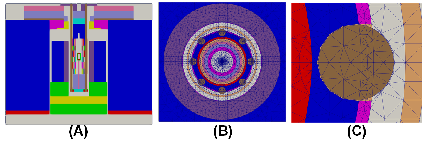
Figure 1: (A) KRUSTY model; (B) the 2D mesh of KRUSTY fuel region with heat pipes; (C) the enlarged framed area in (B).
Listing 1: Input to generate a 2D mesh of irregular shape.
[Mesh]
  [Region2]
    type = ParsedCurveGenerator
    x_formula = 't1:=t;
                 t2:=t-1;
                 t3:=t-2;
                 t4:=t-3;
                 x1:=r_hp_gap*cos(t1*(th1_end-th1_start)+th1_start)+hp_x;
                 x2:=r13*cos(t2*(th2_end-th2_start)+th2_start);
                 x3:=r_slot*cos(t3*(th3_end-th3_start)+th3_start)+hp_x;
                 x4:=r12*cos(t4*(th4_end-th4_start)+th4_start);
                 if(t<1,x1,if(t<2,x2,if(t<3,x3,x4)))'
    y_formula = 't1:=t;
                 t2:=t-1;
                 t3:=t-2;
                 t4:=t-3;
                 y1:=r_hp_gap*sin(t1*(th1_end-th1_start)+th1_start);
                 y2:=r13*sin(t2*(th2_end-th2_start)+th2_start);
                 y3:=r_slot*sin(t3*(th3_end-th3_start)+th3_start);
                 y4:=r12*sin(t4*(th4_end-th4_start)+th4_start);
                 if(t<1,y1,if(t<2,y2,if(t<3,y3,y4)))'
    section_bounding_t_values = '0 1 2 3 4'
    constant_names = 'pi              r12           r13            r_slot          r_hp_gap             hp_x       th1_start     th1_end        th2_start      th2_end           th3_start      th3_end        th4_start       th4_end'
    constant_expressions = '${fparse pi} ${fparse r12} ${fparse r13} ${fparse r_slot} ${fparse r_hp_gap} ${fparse hp_x}    ${fparse pi}  1.4983163888   0.12251793865   0.18118584459  1.5707963268     2.5324547478  0.12272974563       0'
    nums_segments = '4 2 4 4'
    is_closed_loop = true
    # show_info = true
  []
[]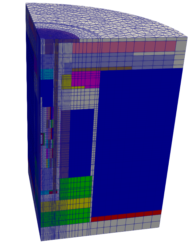
Figure 2: Quarter-core KRUSTY mesh generated using MOOSE
KRUSTY Cross Section Generation
KRUSTY is a small fast spectrum core with a significant amount of neutrons leaking out of the fuel region. The energy spectrum shifts due to neutron leakages and thermal neutrons returning from the reflectors. Therefore, the KRUSTY fuel region was divided into seven radial regions and six axial zones as shown in Figure 1 for applying different cross sections for different fuel regions.
Both Serpent and MC2-3 were used to prepare cross sections for modeling KRUSTY. Sensitivity analysis showed that MC2-3 provides better anisotropic scattering cross sections in the BeO reflector regions, and Serpent provides better cross sections in the fuel region for accounting for the fuel Doppler reactivity feedback. Therefore, a hybrid multigroup cross section set that used MC2-3 cross sections in the reflector region and used Serpent cross sections in other regions was prepared for modeling KRUSTY.
The MC2-3 calculation takes a two-step approach. The first step creates energy self-shielded cross sections and the number of energy-groups used is larger than 1000 groups. These cross sections are imported into an approximated RZ model of KRUSTY as shown in Figure 3. A neutron transport calculation was performed by TWODANT to solve the neutron fluxes in each material region in the RZ model. The neutron fluxes calculated by TWODANT have considered both the neutron leakage effects and spatial self-shielding effects and were imported into the MC2-3 second step. Multigroup cross sections were condensed based on the TWODANT fluxes in each material zone. Table 1 lists the 22-group structure used in the calculations. The MC2-3 input for the first step and the input for TWODANT are documented in mc_s1.in. The MC2-3 input for the second step calculation is similar to the input in the first step but has a different control block as shown in Listing 3.
Figure 3: KRUSTY RZ model for TWODANT calculation
Listing 2: MC2-3 input control block (step 1 calculation)
\$control
     c_group_structure       =ANL1041
     i_number_region         =64
     c_geometry_type         =mixture
     i_scattering_order      =5
     l_twodant               =T
     c_twodant_group         =BG
     l_pendf                 =T
/
Listing 3: MC2-3 input control block (step 2 calculation)
\$control
     c_group_structure       =USER
     i_number_region        =64
     c_geometry_type         =mixture
     c_externalspectrum_ufg  =rzmflx
/
Table 1: The 22-Energy Group Structure for Modeling KRUSTY
| Group # | Upper bond (MeV) | Group # | Upper bond (MeV) | Group # | Upper bond (MeV) |
|---|---|---|---|---|---|
| 1 | 1.4191E+01 | 9 | 1.5034E-02 | 17 | 8.3153E-06 |
| 2 | 1.0000E+01 | 10 | 5.5308E-03 | 18 | 3.9279E-06 |
| 3 | 6.0653E+00 | 11 | 2.0347E-03 | 19 | 1.8554E-06 |
| 4 | 2.2313E+00 | 12 | 7.4852E-04 | 20 | 1.1254E-06 |
| 5 | 8.2085E-01 | 13 | 2.7536E-04 | 21 | 8.7642E-07 |
| 6 | 3.0197E-01 | 14 | 7.8893E-05 | 22 | 4.1745E-07 |
| 7 | 1.1109E-01 | 15 | 3.7267E-05 | ||
| 8 | 4.0868E-02 | 16 | 1.3710E-05 |
Griffin Stand-Alone Neutronic Model
The standalone Griffin input for the neutronic model of KRUSTY is included. Listing 4 shows the mesh block of this input that was used to generate the unstructured file Griffin_mesh.e. The volume for each material region in the mesh file is preserved and made to be consistent with the KRUSTY Serpent reference model. All heat pipe locations are filled. The list in the subdomains block references block ids in the mesh file, and the extra_element_ids is the list of material ids filling the mesh block.
Listing 4: Griffin mesh block for subdomain element IDs assignment.
[Mesh]
 [fmg]
  type = FileMeshGenerator
  file = '../../gold/MESH/Griffin_mesh.e'
 []
 [rot]
  type = TransformGenerator
  input = fmg
  transform = ROTATE
  vector_value = '-90 0 0'
 []
 [id]
   type=SubdomainExtraElementIDGenerator
   input = rot
   subdomains = '1 2 3 4 5 6
                 64 71 72 73
                 8 9 10 11
                 12 1212
                 13 14 15 16 17 18 19
                 20 21 22 23 24
                 2081 2091 2101 2111 2121 2131 2141
                 2082 2092 2102 2112 2122 2132 2142
                 3081 3091 3101 3111 3121 3131 3141
                 3082 3092 3102 3112 3122 3132 3142
                 4081 4091 4101 4111 4121 4131 4141
                 4082 4092 4102 4112 4122 4132 4142'

   extra_element_id_names = 'material_id'
   extra_element_ids ='99 17 11 15 70 18
                       99 6 6 60
                       8 5 10 40
                       51 52
                       4 20 18 40 50 14 13
                       6 7 12 11 9
                       300  310  320  330  340  350  360
                       301  311  321  331  341  351  361
                       202  212  222  232  242  252  262
                       203  213  223  233  243  253  263
                       104  114  124  134  144  154  164
                       105  115  125  135  145  155  165'
  []
Listing 5: Griffin mesh block for coarse mesh definition for CMFD acceleration
  [coarse_mesh]
    type = GeneratedMeshGenerator
    dim= 3
    nx = 20   # about 2 cm may need to adjust
    ny = 20   # about 2 cm may need to adjust
    nz = 40   # about 5 cm may need to adjust to test convergence or performance
    xmin = -2
    xmax =  52
    ymin = -2
    ymax =  52
    zmin = -1
    zmax =  135
  []
   [assign_coarse_id]
     type = CoarseMeshExtraElementIDGenerator
     input = id
     coarse_mesh = coarse_mesh
     extra_element_id_name = coarse_element_id
   []
[]

[AuxVariables]
  [Tf]
    initial_condition = 300
    order = CONSTANT
    family = MONOMIAL
  []

  [Ts]
      initial_condition = 300
      order = CONSTANT
      family = MONOMIAL
  []
[]
[TransportSystems]
  particle = neutron
  equation_type = eigenvalue
  G =22
  VacuumBoundary = 'Core_top Core_bottom Core_outer_boundary'
  ReflectingBoundary = 'Mirror_X_surf Mirror_Y_surf'

  [sn]
    scheme = DFEM-SN
    family = MONOMIAL
    order = FIRST
    AQtype = Gauss-Chebyshev
    NPolar = 3
    NAzmthl = 5

    NA = 3
    sweep_type = asynchronous_parallel_sweeper
    using_array_variable = true
    collapse_scattering  = true
    n_delay_groups = 6
  []
[]

[PowerDensity]
  power = 1275.0
  power_density_variable = power_density
[]

[Executioner]
  type = SweepUpdate

  richardson_abs_tol = 1e-6
  richardson_rel_tol = 1e-20

  richardson_max_its = 1000
  inner_solve_type = GMRes # SI #GMRes

  cmfd_acceleration = true
  coarse_element_id = coarse_element_id
  max_diffusion_coefficient = 10.0
  diffusion_eigen_solver_type = newton
  diffusion_prec_type = lu
  prolongation_type = multiplicative

[]

[Materials]
 [all]
  type=CoupledFeedbackMatIDNeutronicsMaterial
  block='1 2 3 4 5 6
         64 71 72 73
         8 9 10 11
         12 1212
         13 14 15 16 17 18 19
         20 21 22 23 24
         2081 2091 2101 2111 2121 2131 2141
         2082 2092 2102 2112 2122 2132 2142
         3081 3091 3101 3111 3121 3131 3141
         3082 3092 3102 3112 3122 3132 3142
         4081 4091 4101 4111 4121 4131 4141
         4082 4092 4102 4112 4122 4132 4142'
  library_file = '../Serp_hbrid_reflector_updated.xml'
  library_name ='krusty_serpent_ANL_endf70_g22'
  isotopes = 'pseudo'
  densities = '1.0'
  grid_names = 'Tfuel Tsteel'
  grid_variables = 'Tf Ts'
  plus = 1
  is_meter = true
  dbgmat = false
 []
[]

[Outputs]
  csv = true
  exodus = true
  [pgraph]
    type = PerfGraphOutput
    level = 2
  []
[]
The KRUSTY mesh file has modeled 1/4th of the core with reflecting boundaries applied at the center-cut planes. Vacuum boundary conditions are applied on the KRUSTY top, bottom surface, as well as on its outermost radial surface as shown in Listing 6.
Listing 6: Boundary conditions of the Griffin neutronic model for KRUSTY.
[TransportSystems]
  particle = neutron
  equation_type = eigenvalue
  G =22
  VacuumBoundary = 'Core_top Core_bottom Core_outer_boundary'
  ReflectingBoundary = 'Mirror_X_surf Mirror_Y_surf'
Listing 7: Transport system defined in Griffin neutronic model for KRUSTY.
  [sn]
    scheme = DFEM-SN
    family = MONOMIAL
    order = FIRST
    AQtype = Gauss-Chebyshev
    NPolar = 3
    NAzmthl = 5

    NA = 3
    sweep_type = asynchronous_parallel_sweeper
    using_array_variable = true
    collapse_scattering  = true
    n_delay_groups = 6
  []
[]
The Griffin neutronic model solves the and the flux distributions at critical state. Listing 7 shows the transport system block. It used the DFEM-SN solver. Spatial variables are discretized by the DFEM method with shape functions from the first order MONOMIAL family. Angular variables are discretized by the SN method using the Gauss-Chebyshev quadratures. Sensitivity analysis were performed and results were included in Table 2 with different orders of anisotropic scattering terms and different number of angles used in discretizing the angular space. It showed that the calculated was converged after using NPolar=3 angles per octant in the polar direction and NAzmthl=5 angles per octant in the azimuthal direction. With scattering term NA=3, Griffin neutronic model provides better agreement to the Serpent reference among these cases. Including higher scattering order terms may further improve the accuracy of the neutronic results but will require a lot more computational resources. In the Multiphysics model, the neutronic model used NA=3, NPolar=2 and NAzmthl=3 in order to further reduce computational time. As shown in Listing 7, six groups of delayed neutron group families were considered in the numerical calculations. Six delayed neutron data were obtained using Serpent and the values for each group were included in the ISOXML cross section file.
Table 2: Results comparison of different orders of anisotropic scattering terms and different number of angles used in discretizing the angular space.
| Serpent | Griffin (NA=1) | Griffin (NA=2) | Griffin (NA=3) | ||||||
|---|---|---|---|---|---|---|---|---|---|
| SN(1,3) | SN(2,3) | SN(2,5) | SN(3,5) | SN(3,7) | SN(3,5) | SN(3,5) | SN(2,3) | ||
| 1.00592 | 0.99434 | 0.99750 | 0.99751 | 0.99853 | 0.99854 | 1.01125 | 1.00815 | 1.00703 | |
| (pcm) = | 1158 | 842 | 841 | 749 | 738 | -533 | -223 | -111 |
Listing 8 shows the executioner block in the Griffin input where the maximum number of allowed iterations and convergence criteria are specified. The SweepUpdate executioner unique for DFEM-SN was used. The Coarse-Mesh Finite Difference (CMFD) method was deployed to accelerate the DFEM-SN solver. The coarse mesh for the low-order diffusion calculation was a regular mesh that was generated in the mesh block as shown in Listing 5. The maximum diffusion coefficient was set to 10.0, as a limit value facilitating convergence in problems that contain void regions. It can be adjusted and will not significantly affect the accuracy of the results. Newton’s method was used to solve the low-order diffusion equation. Another option to use is the krylovshur method. It was found that it is important to use preconditioners for solving the diffusion equation in order to converge the DFEM-SN solver with CMFD acceleration. In this case, the LU decomposition was used and was found to be effective. The multiplicative prolongation was chosen to update all transport flux moments after solving the low-order diffusion calculation.
Listing 8: Griffin executioner block with options for CMFD acceleration.
[Executioner]
  type = SweepUpdate

  richardson_abs_tol = 1e-6
  richardson_rel_tol = 1e-20

  richardson_max_its = 1000
  inner_solve_type = GMRes # SI #GMRes

  cmfd_acceleration = true
  coarse_element_id = coarse_element_id
  max_diffusion_coefficient = 10.0
  diffusion_eigen_solver_type = newton
  diffusion_prec_type = lu
  prolongation_type = multiplicative
[]Listing 9: The Materials block of the input file
[Materials]
  [all]
    type = CoupledFeedbackMatIDNeutronicsMaterial
    block = '1 2 3 4 5 6
         64 71 72 73
         8 9 10 11
         12 1212
         13 14 15 16 17 18 19
         20 21 22 23 24
         2081 2091 2101 2111 2121 2131 2141
         2082 2092 2102 2112 2122 2132 2142
         3081 3091 3101 3111 3121 3131 3141
         3082 3092 3102 3112 3122 3132 3142
         4081 4091 4101 4111 4121 4131 4141
         4082 4092 4102 4112 4122 4132 4142'
    library_file = '../Serp_hbrid_reflector_updated.xml'
    library_name = 'krusty_serpent_ANL_endf70_g22'
    isotopes = 'pseudo'
    densities = '1.0'
    grid_names = 'Tfuel Tsteel'
    grid_variables = 'Tf Ts'
    plus = 1
    is_meter = true
    dbgmat = false
  []
[]Listing 10: AuxVariables defined for cross section grid indices in Griffin neutronic model for KRUSTY
[AuxVariables]
  [Tf]
    initial_condition = 300
    order = CONSTANT
    family = MONOMIAL
  []

  [Ts]
    initial_condition = 300
    order = CONSTANT
    family = MONOMIAL
  []
[]Listing 9 shows the material block in the Griffin input. The CoupledFeedbackMatIDNeutronicsMaterial, which interpolates multigroup cross sections on-the-fly among a tabulated cross section set, was used for multiphysics simulation. The material ID was read from the mesh block. The hybrid cross section set that was generated from Serpent and MC2-3 was used. The cross sections within the file are zone-averaged macroscopic cross sections. Therefore, the isotopes were assigned to be ‘pseudo’ and its density was 1.0.
The cross section set included a 2-D cross section table. The indices to lookup the 2-D table were the fuel temperature “Tf” and the structure temperature “Ts” that covers all other nonfuel regions. The state temperature points include fuel at 300 K, 600 K, 800 K, 1000 K and 1200 K and the structure material at 300 K, 600 K, 800 K and 1000 K, respectively. Listing 10 shows how different fuel and structure temperatures can be specified in the stand-alone neutronic calculations.
Finally, Listing 11 shows the steps to tally the axial power distribution in the KRUSTY innermost (“r1”) layer. To integrate the fission power within each fuel layer (seven radial layers), an AuxVariable in MOOSE that can be processed by the VectorPostprocessor was first defined to hold the layer-integrated total fission power for the axial regions within that layer as shown in the first block of Listing 11. A UserObject as shown in the second block of Listing 11 was necessary to perform the actual integration among the different axial layers. The integrated values were then placed into the AuxVariable as shown in the third block of Listing 11 and were printed out by the VectorPostprocessor as shown in the fourth block of Listing 11.
Listing 11: Output blocks in Griffin neutronic model for KRUSTY to tally the power density in one of the fuel region: AuxVariable block; UserObject block; AuxKernel block; VectorPostprocessor block
[AuxVariables]
  [axial_r1_z]
    order = FIRST
    family = MONOMIAL
  []
[]
[UserObjects]
  [axial_r1_z]
    type = LayeredIntegral
    variable = power_density
    direction = z
    bounds = '35 36 37 38 39 40.083435 41.16687 42.250305 43.33374 43.97763
              44.62152 44.85012 45.11512 45.38012 46.19006 47 48.09006 49.18012
              49.71012 49.95142 50.80945 51.66748 52.50061 53.33374 54.16687
              55 55.8416779 56.6833558 57.5250337 58.3667116 59.1839658 60.00122'
    block = '2081 2082 3081 3082 4081 4082'
  []
[]
[AuxKernels]
  [axial_r1_z]
    type = SpatialUserObjectAux
    variable = axial_r1_z
    execute_on = timestep_end
    user_object = axial_r1_z
  []
[]
[VectorPostprocessors]
  [axial_r1_z_elm]
    type = ElementValueSampler
    variable = axial_r1_z
    sort_by = z
    execute_on = timestep_end
  []
[]
BISON Thermal-Mechanical Model
BISON was utilized to conduct thermo-mechanical simulations. In KRUSTY, the fuel disk and its radial shield hung down from the top stainless-steel plates. The bottom and radial reflectors sat on a movable platen below the fuel disk and were pushed up into the radial shield region to reach criticality. With very good insulation of the fuel disk, the top and bottom plates were about room temperature. Therefore, the reactor core was modeled between the fixed top and bottom surfaces with no total displacement in the axial direction but allowing radial thermal expansion or contraction. The top and bottom parts of KRUSTY were connected by “soft materials” to represent the vacuum and air region surrounding the fuel disk. In the KRUSTY thermo-mechanical model, the radial reflector expands upward into the “soft material” region when the fission power increases, and the fuel expansion is downward resulting in more part of fuel covered by the reflectors. Convective heat flux boundary conditions (h=5 W/m²·K) were applied to the top, bottom, and side surfaces of the core.
For a thermo-mechanical model, thermophysical properties (i.e., thermal conductivity, density, specific heat, and thermal expansion coefficient) and mechanical properties (i.e., elastic modulus) of all the involved components are needed. Table 3 lists the BISON/MOOSE models used for thermo-mechanical simulations. BISON doesn't include models for KRUSTY’s U-7.65Mo fuel material, so the thermal conductivity of U-10Mo and specific heat of U-8Mo are currently applied. Other thermal and mechanical attributes for U-7.65Mo and B4C were sourced from the open literature or based on certain assumptions. The displacements in the “soft materials” regions are not solved using MOOSE’s solid mechanics solver as the solid components. Instead, simple diffusion is used for these regions to simply propagate the deformation of the solid components.
Table 3: Thermophysical and Elasticity Models Used for Thermo-Mechanical Simulation
| BISON/MOOSE models | Materials | Description |
|---|---|---|
| HeatConductionMaterial | UMo | Thermal properties of UMo (Parida et al., 2001; Burkes et al., 2010) |
| BeOThermal | BeO | Thermal properties of BeO |
| BeOElasticityTensor | BeO | Young's modulus and Poisson's ratio for BeO |
| BeOThermalExpansionEigenstrain | BeO | Computation of eigenstrain due to thermal expansion in BeO |
| SS316Thermal | SS | Thermal properties of SS-316 |
| SS316ElasticityTensor | SS | Young's modulus and Poisson's ratio for SS-316 |
| SS316ThermalExpansion Eigenstrain | SS | Computation of eigenstrain due to thermal expansion in SS316 |
As mentioned above, in the KRUSTY design, a thin insulation layer is used to thermally isolate the fuel from other components to reduce the loss of energy through heat transfer from fuel to reactor external surface. In order to simulate the thermal behavior of this thin insulation layer, MOOSE’s interface kernel is adopted to model the thermal resistance of the insulation layer without the need to explicitly mesh the thin structure. The thermal resistance of the insulation layer is tuned to match the reported behavior of KRUSTY (i.e., 30 W power leading to 200ºC fuel temperature).
MOOSE Multiphysics Coupling
In KRUSTY warm critical experiments, the power excursion transient was initiated by shifting the radial reflector of KRUSTY upward to insert positive reactivity when the reactor was in a cold/critical state (Poston et al., 2020). This VTB model includes the multiphysics model prepared for modeling this reactivity insertion test. A two-level MOOSE MultiApps hierarchy which tightly couples the aforementioned Griffin neutronics model and BISON thermo-mechanical model has been developed to simulate the KRUSTY warm critical tests. Griffin is set as the parent (main) application and uses the DFEM-SN(2,3) solver with CMFD acceleration and NA=3 (anisotropic scattering order), while BISON is set as the child application.
The power density profile, initially calculated by Griffin, is then transferred to BISON. In BISON, thermo-mechanical computations take place, allowing for the determination of temperature distribution within all solid components. This subsequently leads to the calculation of thermal expansion. Both the fuel temperature profile and displacement field are then sent back to Griffin as feedback for the neutronics simulation. The coupling of these two applications occurs through fixed point iteration. Notably, in this calculation, all heat is passively removed through the external boundary of the reactor, as no heat pipes are involved.
The movement of the axial reflector to insert the reactivity was modeled by forcing a Dirichlet boundary condition on the bottom of the solid assembly that includes the axial reflector to allow BISON to calculate the consequent displacement field through solving solid mechanics equations. Two steady-state eigenvalue calculations were included in the VTB model. These calculations were performed to confirm that an adequate amount of external reactivity was introduced for initiating the transient. The first one corresponds to the initial steady state for future transient simulation, and the second steady state corresponds to the first step of the transient after the reflector is shifted upward. In this calculation, the bias in the axial direction was set in the BISON input as shown in Listing 12 to generate the displacement in the mesh. The displacements were passed to Griffin neutronic for calculating the total reactivity inserted into the reactor using the MultiApp coupling framework.
Listing 12: Bison inputs for modeling the movement of the axial reflectors in KRUSTY warm critical experiments
reflector_disp = 0.0 # use 1.48e-3 for reactivity insertion
[BCs]
  [BottomSSFixZ]
    type = DirichletBC
    variable = disp_z
    boundary = 'ss_bot'
    value = ${reflector_disp}
  []
[]
References
- Douglas E Burkes, Cynthia A Papesch, Andrew P Maddison, Thomas Hartmann, and Francine J Rice.
Thermo-physical properties of du–10 wt.% mo alloys.
Journal of Nuclear Materials, 403(1-3):160–166, 2010.[BibTeX]
@article{Burkes2010, author = "Burkes, Douglas E and Papesch, Cynthia A and Maddison, Andrew P and Hartmann, Thomas and Rice, Francine J", title = "Thermo-physical properties of DU--10 wt.\\% Mo alloys", journal = "Journal of Nuclear Materials", volume = "403", number = "1-3", pages = "160--166", year = "2010", publisher = "Elsevier" } - SC Parida, Sonali Dash, Z Singh, R Prasad, and V Venugopal.
Thermodynamic studies on uranium–molybdenum alloys.
Journal of Physics and Chemistry of Solids, 62(3):585–597, 2001.[BibTeX]
@article{Parida2001, author = "Parida, SC and Dash, Sonali and Singh, Z and Prasad, R and Venugopal, V", title = "Thermodynamic studies on uranium--molybdenum alloys", journal = "Journal of Physics and Chemistry of Solids", volume = "62", number = "3", pages = "585--597", year = "2001", publisher = "Elsevier" } - David I Poston, Marc A Gibson, Patrick R McClure, and Rene G Sanchez.
Results of the krusty warm critical experiments.
Nuclear Technology, 206(sup1):S78–S88, 2020.[BibTeX]
@article{Poston2020_1,
    author = "Poston, David I and Gibson, Marc A and McClure, Patrick R and Sanchez, Rene G",
    title = "Results of the KRUSTY warm critical experiments",
    journal = "Nuclear Technology",
    volume = "206",
    number = "sup1",
    pages = "S78--S88",
    year = "2020",
    publisher = "Taylor \\& Francis"
}
(microreactors/KRUSTY/MESH/KRUSTY_mesh_gen_griffin.i)
################################################################################
## NEAMS Micro-Reactor Application Driver ##
## KRUSTY Mesh Generation ##
## Input File Using MOOSE Framework/Reactor Module Mesh Generators ##
## Original Mesh for Griffin ##
## Please contact the authors for mesh generation issues: ##
## - Dr. Kun Mo ([email protected]) ##
## - Dr. Soon Kyu Lee ([email protected]) ##
################################################################################
################################################################################
# Geometry Info.
################################################################################
# Radii used in parsed curve generators to model different component geometries.
################################################################################
r1 = 0.33655
r2 = 0.559435
r3 = 0.69
r5 = 1.0033
r6 = 1.412875
r7 = 1.9939
r8 = 2.6
r9 = 3.175
r10 = 3.6
r11 = 4.1
r12 = 4.45168
r13 = 5.285907
r14 = 5.4991
r15 = 6.0325
r16 = 6.35
r17 = 7.049135
r18 = 7.140575
r19 = 7.3025
r20 = 7.874
r21 = 10.4775
r22 = 12.7
r23 = 15.22413
r24 = 19.05
r25 = 19.84375
r26 = 20.48002
r27 = 50.96002
################################################################################
# Top Plate Parameters:
################################################################################
plate_wirth_half = 31.75
plate_length_half = 38.1
################################################################################
# Top Bar Parameters:
################################################################################
bar_length_half = 46.99
################################################################################
# Heat Pipe Parameters:
################################################################################
r_hp = 0.635
r_hp_gap = 0.6477
hp_x = 5.19938
r_slot = 0.9525
################################################################################
# Component Hights
# (h is the distance of H(x)-H(x-1); for example, h2 = -27.935-(-35)):
################################################################################
# h --------------- Height # Notes
# h1 =0 #1 -35
h2 =7.065 #2 -27.935
# h3 =0 #3 -27.935
h4 =2.3774 #4 -25.5576
h5 =0.1626 #5 -25.395
h6 =4.9174 #6 -20.4776
h7 =5.08 #7 -15.3976
h8 =1.2625 #8 -14.1351
h9 =2.0701 #9 -12.065
h10=1.27 #10 -10.795
h11=0.635 #11 -10.16
h12=4.9224 #12 -5.2376
h13=5.08012 #13 -0.15748
h14=0.15748 #14 0 # Fuel Zone Start
h15=4 #15 4
h16=4.33374 #16 8.33374 # Bottom Fuel Zone End & Middle Fuel Zone Start
h17=1.28778 #17 9.62152
h18=0.2286 #18 9.85012
h19=0.53 #19 10.38012
h20=1.61988 #20 12
h21=2.18012 #21 14.18012
h22=0.53 #22 14.71012
h23=0.2413 #23 14.95142
h24=1.71606 #24 16.66748 # Middle Fuel Zone End & Top Fuel Zone Start
h25=3.33252 #25 20
h26=3.36671 #26 23.36671
h27=1.63451 #27 25.00122 # Top Fuel Zone End
h28=3.8354 #28 28.83662
h29=2.52468 #29 31.3613
h30=0.96266 #30 32.32396
h31=2.83726 #31 35.16122
h32=1.60774 #32 36.76896
h33=0.94234 #33 37.7113
h34=1.25992 #34 38.97122
h35=1.905 #35 40.87622
h36=1.91508 #36 42.7913
h37=1.27 #37 44.0613
h38=3.81008 #38 47.87138
h39=1.27 #39 49.14138
################################################################################
# Block ID Information
fuel_all = '2081 2082 2091 2092 2101 2102 2111 2112 2121 2122 2131 2132 2141 2142 3081 3082 3091 3092 3101 3102 3111 3112 3121 3122 3131 3132 3141 3142 4081 4082 4091 4092 4101 4102 4111 4112 4121 4122 4131 4132 4141 4142'
Be_all = '14'
Al_all = '11 13 16'
hp_all = '10'
beo_all = '12 1212 17 9'
ss_all = '2 3 4 6 71 72 73 8 15 18 19 20 22 23 24'
b4c_all = '5 21'
air_all = '1'
hp_fuel_gap_all = '64'
################################################################################
################################################################################
# Starting of the Mesh Input Block
################################################################################
[Mesh]
# final_generator=Extrude
################################################################################
# 2D Component Generation Near the Heat Pipe (Region1-26)
# Due to the complex geometries of the Krusty components, various Regions are
# outlined with the ParsedCurveGenerator and meshed with the XYDelaunayGenerator.
# Each region holds multiple components when axially extruded.
#
# The following key components are comprised of these Regions:
# Fuel: Region 1, 2, 3, 11, 12, 13
# Heat Pipe (HP): Region 8, 9, 10
# HP and Fuel Gap: Region 5, 6, 7
# BeO Reflector: Region 18, 19, 20, 24, 25, 26
################################################################################
[Region1]
type = ParsedCurveGenerator
x_formula = 't1:=t;
t2:=t-1;
x1:=r12*cos(t1*(th1_end-th1_start)+th1_start);
x2:=r_slot*cos(t2*(th2_end-th2_start)+th2_start)+hp_x;
if(t<1,x1,x2)'
y_formula = 't1:=t;
t2:=t-1;
y1:=r12*sin(t1*(th1_end-th1_start)+th1_start);
y2:=r_slot*sin(t2*(th2_end-th2_start)+th2_start);
if(t<1,y1,y2)'
section_bounding_t_values = '0 1 2'
constant_names = 'pi r12 r_slot hp_x th1_start th1_end th2_start th2_end'
constant_expressions = '${fparse pi} ${fparse r12} ${fparse r_slot} ${fparse hp_x} 0 0.12272974563 2.5324547478 ${fparse pi}'
nums_segments = '4 4'
is_closed_loop = true
[]
[Region1_mesh]
type = XYDelaunayGenerator
boundary = 'Region1'
# add_nodes_per_boundary_segment = 2
refine_boundary = false
desired_area = 0.1
output_boundary = 9527
output_subdomain_name = 101
[]
[Region2]
type = ParsedCurveGenerator
x_formula = 't1:=t;
t2:=t-1;
t3:=t-2;
t4:=t-3;
x1:=r_hp_gap*cos(t1*(th1_end-th1_start)+th1_start)+hp_x;
x2:=r13*cos(t2*(th2_end-th2_start)+th2_start);
x3:=r_slot*cos(t3*(th3_end-th3_start)+th3_start)+hp_x;
x4:=r12*cos(t4*(th4_end-th4_start)+th4_start);
if(t<1,x1,if(t<2,x2,if(t<3,x3,x4)))'
y_formula = 't1:=t;
t2:=t-1;
t3:=t-2;
t4:=t-3;
y1:=r_hp_gap*sin(t1*(th1_end-th1_start)+th1_start);
y2:=r13*sin(t2*(th2_end-th2_start)+th2_start);
y3:=r_slot*sin(t3*(th3_end-th3_start)+th3_start);
y4:=r12*sin(t4*(th4_end-th4_start)+th4_start);
if(t<1,y1,if(t<2,y2,if(t<3,y3,y4)))'
section_bounding_t_values = '0 1 2 3 4'
constant_names = 'pi r12 r13 r_slot r_hp_gap hp_x th1_start th1_end th2_start th2_end th3_start th3_end th4_start th4_end'
constant_expressions = '${fparse pi} ${fparse r12} ${fparse r13} ${fparse r_slot} ${fparse r_hp_gap} ${fparse hp_x} ${fparse pi} 1.4983163888 0.12251793865 0.18118584459 1.5707963268 2.5324547478 0.12272974563 0'
nums_segments = '4 2 4 4'
is_closed_loop = true
# show_info = true
[]
[Region2_mesh]
type = XYDelaunayGenerator
boundary = 'Region2'
# add_nodes_per_boundary_segment = 2
refine_boundary = false
desired_area = 0.1
output_boundary=9527
output_subdomain_name = 102
[]
[Region3]
type = ParsedCurveGenerator
x_formula = 'tm:=if(t=4,0,t);
t1:=tm;
t2:=tm-1;
t3:=tm-2;
t4:=tm-3;
x1:=r_hp_gap*cos(t1*(th1_end-th1_start)+th1_start)+hp_x;
x2:=r14*cos(t2*(th2_end-th2_start)+th2_start);
x3:=t3*(th3_end-th3_start)+th3_start;
x4:=r13*cos(t4*(th4_end-th4_start)+th4_start);
if(tm<1,x1,if(tm<2,x2,if(tm<3,x3,x4)))'
y_formula = 'tm:=if(t=4,0,t);
t1:=tm;
t2:=tm-1;
t3:=tm-2;
t4:=tm-3;
y1:=r_hp_gap*sin(t1*(th1_end-th1_start)+th1_start);
y2:=r14*sin(t2*(th2_end-th2_start)+th2_start);
y3:=r_slot;
y4:=r13*sin(t4*(th4_end-th4_start)+th4_start);
if(tm<1,y1,if(tm<2,y2,if(tm<3,y3,y4)))'
section_bounding_t_values = '0 1 2 3 4'
constant_names = 'pi r12 r13 r14 r15 r_slot r_hp_gap hp_x th1_start th1_end th2_start th2_end th3_start th3_end th4_start th4_end'
constant_expressions = '${fparse pi} ${fparse r12} ${fparse r13} ${fparse r14} ${fparse r15} ${fparse r_slot} ${fparse r_hp_gap} ${fparse hp_x} 1.4983163888 1.14417605 0.1074325051 0.1740881695 5.41598048 5.19938 0.18118584 0.12251793'
nums_segments = '2 2 2 2'
is_closed_loop = true
[]
[Region3_mesh]
type = XYDelaunayGenerator
boundary = 'Region3'
# add_nodes_per_boundary_segment = 2
refine_boundary = false
desired_area = 0.01
output_boundary=9527
output_subdomain_name = 103
[]
[Region4]
type = ParsedCurveGenerator
x_formula = 't1:=t;
t2:=t-1;
t3:=t-2;
t4:=t-3;
x1:=r15*cos(t1*(th1_end-th1_start)+th1_start);
x2:=t2*(th2_end-th2_start)+th2_start;
x3:=r14*cos(t3*(th3_end-th3_start)+th3_start);
x4:=r_hp_gap*cos(t4*(th4_end-th4_start)+th4_start)+hp_x;
if(t<1,x1,if(t<2,x2,if(t<3,x3,x4)))'
y_formula = 't1:=t;
t2:=t-1;
t3:=t-2;
t4:=t-3;
y1:=r15*sin(t1*(th1_end-th1_start)+th1_start);
y2:=r_slot;
y3:=r14*sin(t3*(th3_end-th3_start)+th3_start);
y4:=r_hp_gap*sin(t4*(th4_end-th4_start)+th4_start);
if(t<1,y1,if(t<2,y2,if(t<3,y3,y4)))'
section_bounding_t_values = '0 1 2 3 4'
constant_names = 'pi r12 r13 r14 r15 r_slot r_hp_gap hp_x th1_start th1_end th2_start th2_end th3_start th3_end th4_start th4_end'
constant_expressions = '${fparse pi} ${fparse r12} ${fparse r13} ${fparse r14} ${fparse r15} ${fparse r_slot} ${fparse r_hp_gap} ${fparse hp_x} 0 0.15855828 5.9568280 5.41598048 0.1740881695 0.1074325051 1.14417605 0 '
nums_segments = '3 2 2 4'
is_closed_loop = true
[]
[Region4_mesh]
type = XYDelaunayGenerator
boundary = 'Region4'
# add_nodes_per_boundary_segment = 2
refine_boundary = false
desired_area = 0.1
output_boundary = 9527
output_subdomain_name = 104
[]
[Region21]
type = ParsedCurveGenerator
x_formula = 'tm:=if(t=4,0,t);
t1:=tm;
t2:=tm-1;
t3:=tm-2;
t4:=tm-3;
x1:=r16*cos(t1*(th1_end-th1_start)+th1_start);
x2:=t2*(th2_end-th2_start)+th2_start;
x3:=r15*cos(t3*(th3_end-th3_start)+th3_start);
x4:=t4*(th4_end-th4_start)+th4_start;
if(tm<1,x1,if(tm<2,x2,if(tm<3,x3,x4)))'
y_formula = 'tm:=if(t=4,0,t);
t1:=tm;
t2:=tm-1;
t3:=tm-2;
t4:=tm-3;
y1:=r16*sin(t1*(th1_end-th1_start)+th1_start);
y2:=r_slot;
y3:=r15*sin(t3*(th3_end-th3_start)+th3_start);
y4:=0;
if(tm<1,y1,if(tm<2,y2,if(tm<3,y3,y4)))'
section_bounding_t_values = '0 1 2 3 4'
constant_names = 'pi r12 r13 r14 r15 r16 r17 r18 r19 r20 r21 r_slot r_hp r_hp_gap hp_x th1_start th1_end th2_start th2_end th3_start th3_end th4_start th4_end'
constant_expressions = '${fparse pi} ${fparse r12} ${fparse r13} ${fparse r14} ${fparse r15} ${fparse r16} ${fparse r17} ${fparse r18} ${fparse r19} ${fparse r20} ${fparse r21} ${fparse r_slot} ${fparse r_hp} ${fparse r_hp_gap} ${fparse hp_x} 0 ${fparse asin(r_slot/r16)} ${fparse sqrt(r16^2-r_slot^2)} ${fparse sqrt(r15^2-r_slot^2)} ${fparse asin(r_slot/r15)} 0 ${fparse r15} ${fparse r16}'
nums_segments = '3 1 3 1'
is_closed_loop = true
[]
[Region21_mesh]
type = XYDelaunayGenerator
boundary = 'Region21'
# add_nodes_per_boundary_segment = 2
refine_boundary = false
desired_area = 0.3
output_boundary = 9527
output_subdomain_name = 121
[]
[Region22]
type = ParsedCurveGenerator
x_formula = 'tm:=if(t=4,0,t);
t1:=tm;
t2:=tm-1;
t3:=tm-2;
t4:=tm-3;
x1:=r17*cos(t1*(th1_end-th1_start)+th1_start);
x2:=t2*(th2_end-th2_start)+th2_start;
x3:=r16*cos(t3*(th3_end-th3_start)+th3_start);
x4:=t4*(th4_end-th4_start)+th4_start;
if(tm<1,x1,if(tm<2,x2,if(tm<3,x3,x4)))'
y_formula = 'tm:=if(t=4,0,t);
t1:=tm;
t2:=tm-1;
t3:=tm-2;
t4:=tm-3;
y1:=r17*sin(t1*(th1_end-th1_start)+th1_start);
y2:=r_slot;
y3:=r16*sin(t3*(th3_end-th3_start)+th3_start);
y4:=0;
if(tm<1,y1,if(tm<2,y2,if(tm<3,y3,y4)))'
section_bounding_t_values = '0 1 2 3 4'
constant_names = 'pi r12 r13 r14 r15 r16 r17 r18 r19 r20 r21 r_slot r_hp r_hp_gap hp_x th1_start th1_end th2_start th2_end th3_start th3_end th4_start th4_end'
constant_expressions = '${fparse pi} ${fparse r12} ${fparse r13} ${fparse r14} ${fparse r15} ${fparse r16} ${fparse r17} ${fparse r18} ${fparse r19} ${fparse r20} ${fparse r21} ${fparse r_slot} ${fparse r_hp} ${fparse r_hp_gap} ${fparse hp_x} 0 ${fparse asin(r_slot/r17)} ${fparse sqrt(r17^2-r_slot^2)} ${fparse sqrt(r16^2-r_slot^2)} ${fparse asin(r_slot/r16)} 0 ${fparse r16} ${fparse r17}'
nums_segments = '3 2 3 2'
is_closed_loop = true
[]
[Region22_mesh]
type = XYDelaunayGenerator
boundary = 'Region22'
# add_nodes_per_boundary_segment = 2
refine_boundary = false
desired_area = 0.3
output_boundary = 9527
output_subdomain_name = 122
[]
[Region23]
type = ParsedCurveGenerator
x_formula = 'tm:=if(t=4,0,t);
t1:=tm;
t2:=tm-1;
t3:=tm-2;
t4:=tm-3;
x1:=r18*cos(t1*(th1_end-th1_start)+th1_start);
x2:=t2*(th2_end-th2_start)+th2_start;
x3:=r17*cos(t3*(th3_end-th3_start)+th3_start);
x4:=t4*(th4_end-th4_start)+th4_start;
if(tm<1,x1,if(tm<2,x2,if(tm<3,x3,x4)))'
y_formula = 'tm:=if(t=4,0,t);
t1:=tm;
t2:=tm-1;
t3:=tm-2;
t4:=tm-3;
y1:=r18*sin(t1*(th1_end-th1_start)+th1_start);
y2:=r_slot;
y3:=r17*sin(t3*(th3_end-th3_start)+th3_start);
y4:=0;
if(tm<1,y1,if(tm<2,y2,if(tm<3,y3,y4)))'
section_bounding_t_values = '0 1 2 3 4'
constant_names = 'pi r12 r13 r14 r15 r16 r17 r18 r19 r20 r21 r_slot r_hp r_hp_gap hp_x th1_start th1_end th2_start th2_end th3_start th3_end th4_start th4_end'
constant_expressions = '${fparse pi} ${fparse r12} ${fparse r13} ${fparse r14} ${fparse r15} ${fparse r16} ${fparse r17} ${fparse r18} ${fparse r19} ${fparse r20} ${fparse r21} ${fparse r_slot} ${fparse r_hp} ${fparse r_hp_gap} ${fparse hp_x} 0 ${fparse asin(r_slot/r18)} ${fparse sqrt(r18^2-r_slot^2)} ${fparse sqrt(r17^2-r_slot^2)} ${fparse asin(r_slot/r17)} 0 ${fparse r17} ${fparse r18}'
nums_segments = '3 1 3 1'
is_closed_loop = true
[]
[Region23_mesh]
type = XYDelaunayGenerator
boundary = 'Region23'
# add_nodes_per_boundary_segment = 2
refine_boundary = false
desired_area = 0.1
output_boundary = 9527
output_subdomain_name = 123
[]
[Region24]
type = ParsedCurveGenerator
x_formula = 'tm:=if(t=4,0,t);
t1:=tm;
t2:=tm-1;
t3:=tm-2;
t4:=tm-3;
x1:=r19*cos(t1*(th1_end-th1_start)+th1_start);
x2:=t2*(th2_end-th2_start)+th2_start;
x3:=r18*cos(t3*(th3_end-th3_start)+th3_start);
x4:=t4*(th4_end-th4_start)+th4_start;
if(tm<1,x1,if(tm<2,x2,if(tm<3,x3,x4)))'
y_formula = 'tm:=if(t=4,0,t);
t1:=tm;
t2:=tm-1;
t3:=tm-2;
t4:=tm-3;
y1:=r19*sin(t1*(th1_end-th1_start)+th1_start);
y2:=r_slot;
y3:=r18*sin(t3*(th3_end-th3_start)+th3_start);
y4:=0;
if(tm<1,y1,if(tm<2,y2,if(tm<3,y3,y4)))'
section_bounding_t_values = '0 1 2 3 4'
constant_names = 'pi r12 r13 r14 r15 r16 r17 r18 r19 r20 r21 r_slot r_hp r_hp_gap hp_x th1_start th1_end th2_start th2_end th3_start th3_end th4_start th4_end'
constant_expressions = '${fparse pi} ${fparse r12} ${fparse r13} ${fparse r14} ${fparse r15} ${fparse r16} ${fparse r17} ${fparse r18} ${fparse r19} ${fparse r20} ${fparse r21} ${fparse r_slot} ${fparse r_hp} ${fparse r_hp_gap} ${fparse hp_x} 0 ${fparse asin(r_slot/r19)} ${fparse sqrt(r19^2-r_slot^2)} ${fparse sqrt(r18^2-r_slot^2)} ${fparse asin(r_slot/r18)} 0 ${fparse r18} ${fparse r19}'
nums_segments = '3 1 3 1'
is_closed_loop = true
[]
[Region24_mesh]
type = XYDelaunayGenerator
boundary = 'Region24'
# add_nodes_per_boundary_segment = 2
refine_boundary = false
desired_area = 0.1
output_boundary = 9527
output_subdomain_name = 124
[]
[Region25]
type = ParsedCurveGenerator
x_formula = 'tm:=if(t=4,0,t);
t1:=tm;
t2:=tm-1;
t3:=tm-2;
t4:=tm-3;
x1:=r20*cos(t1*(th1_end-th1_start)+th1_start);
x2:=t2*(th2_end-th2_start)+th2_start;
x3:=r19*cos(t3*(th3_end-th3_start)+th3_start);
x4:=t4*(th4_end-th4_start)+th4_start;
if(tm<1,x1,if(tm<2,x2,if(tm<3,x3,x4)))'
y_formula = 'tm:=if(t=4,0,t);
t1:=tm;
t2:=tm-1;
t3:=tm-2;
t4:=tm-3;
y1:=r20*sin(t1*(th1_end-th1_start)+th1_start);
y2:=r_slot;
y3:=r19*sin(t3*(th3_end-th3_start)+th3_start);
y4:=0;
if(tm<1,y1,if(tm<2,y2,if(tm<3,y3,y4)))'
section_bounding_t_values = '0 1 2 3 4'
constant_names = 'pi r12 r13 r14 r15 r16 r17 r18 r19 r20 r21 r_slot r_hp r_hp_gap hp_x th1_start th1_end th2_start th2_end th3_start th3_end th4_start th4_end'
constant_expressions = '${fparse pi} ${fparse r12} ${fparse r13} ${fparse r14} ${fparse r15} ${fparse r16} ${fparse r17} ${fparse r18} ${fparse r19} ${fparse r20} ${fparse r21} ${fparse r_slot} ${fparse r_hp} ${fparse r_hp_gap} ${fparse hp_x} 0 ${fparse asin(r_slot/r20)} ${fparse sqrt(r20^2-r_slot^2)} ${fparse sqrt(r19^2-r_slot^2)} ${fparse asin(r_slot/r19)} 0 ${fparse r19} ${fparse r20}'
nums_segments = '3 2 3 2'
is_closed_loop = true
[]
[Region25_mesh]
type = XYDelaunayGenerator
boundary = 'Region25'
# add_nodes_per_boundary_segment = 2
refine_boundary = false
desired_area = 0.3
output_boundary = 9527
output_subdomain_name = 125
[]
[Region26]
type = ParsedCurveGenerator
x_formula = 'tm:=if(t=4,0,t);
t1:=tm;
t2:=tm-1;
t3:=tm-2;
t4:=tm-3;
x1:=r21*cos(t1*(th1_end-th1_start)+th1_start);
x2:=t2*(th2_end-th2_start)+th2_start;
x3:=r20*cos(t3*(th3_end-th3_start)+th3_start);
x4:=t4*(th4_end-th4_start)+th4_start;
if(tm<1,x1,if(tm<2,x2,if(tm<3,x3,x4)))'
y_formula = 'tm:=if(t=4,0,t);
t1:=tm;
t2:=tm-1;
t3:=tm-2;
t4:=tm-3;
y1:=r21*sin(t1*(th1_end-th1_start)+th1_start);
y2:=r_slot;
y3:=r20*sin(t3*(th3_end-th3_start)+th3_start);
y4:=0;
if(tm<1,y1,if(tm<2,y2,if(tm<3,y3,y4)))'
section_bounding_t_values = '0 1 2 3 4'
constant_names = 'pi r12 r13 r14 r15 r16 r17 r18 r19 r20 r21 r_slot r_hp r_hp_gap hp_x th1_start th1_end th2_start th2_end th3_start th3_end th4_start th4_end'
constant_expressions = '${fparse pi} ${fparse r12} ${fparse r13} ${fparse r14} ${fparse r15} ${fparse r16} ${fparse r17} ${fparse r18} ${fparse r19} ${fparse r20} ${fparse r21} ${fparse r_slot} ${fparse r_hp} ${fparse r_hp_gap} ${fparse hp_x} 0 ${fparse asin(r_slot/r21)} ${fparse sqrt(r21^2-r_slot^2)} ${fparse sqrt(r20^2-r_slot^2)} ${fparse asin(r_slot/r20)} 0 ${fparse r20} ${fparse r21}'
nums_segments = '3 6 3 6'
is_closed_loop = true
[]
[Region26_mesh]
type = XYDelaunayGenerator
boundary = 'Region26'
# add_nodes_per_boundary_segment = 2
refine_boundary = false
desired_area = 0.2
output_boundary = 9527
output_subdomain_name = 126
[]
[Stitch_Region1_to_4_and_21_to_26]
type = StitchedMeshGenerator
inputs = 'Region1_mesh Region2_mesh Region3_mesh Region4_mesh Region21_mesh Region22_mesh Region23_mesh Region24_mesh Region25_mesh Region26_mesh'
clear_stitched_boundary_ids = true
prevent_boundary_ids_overlap =false
stitch_boundaries_pairs = '9527 9527; 9527 9527; 9527 9527; 9527 9527; 9527 9527; 9527 9527; 9527 9527; 9527 9527; 9527 9527'
subdomain_remapping = false # see idaholab/moose#30802
[]
[Region5]
type = ParsedCurveGenerator
x_formula = 't1:=t;
t2:=t-1;
t3:=t-2;
x1:=r_hp*cos(t1*(th1_end-th1_start)+th1_start)+hp_x;
x2:=r13*cos(t2*(th2_end-th2_start)+th2_start);
x3:=r_hp_gap*cos(t3*(th3_end-th3_start)+th3_start)+hp_x;
if(t<1,x1,if(t<2,x2,x3))'
y_formula = 't1:=t;
t2:=t-1;
t3:=t-2;
y1:=r_hp*sin(t1*(th1_end-th1_start)+th1_start);
y2:=r13*sin(t2*(th2_end-th2_start)+th2_start);
y3:=r_hp_gap*sin(t3*(th3_end-th3_start)+th3_start);
if(t<1,y1,if(t<2,y2,y3))'
section_bounding_t_values = '0 1 2 3'
constant_names = 'pi r12 r13 r14 r15 r_slot r_hp r_hp_gap hp_x th1_start th1_end th2_start th2_end th3_start th3_end'
constant_expressions = '${fparse pi} ${fparse r12} ${fparse r13} ${fparse r14} ${fparse r15} ${fparse r_slot} ${fparse r_hp} ${fparse r_hp_gap} ${fparse hp_x} ${fparse pi} 1.494390157 0.120068556 0.12251793865 1.4983163888 ${fparse pi}'
nums_segments = '4 1 4'
is_closed_loop = true
[]
[Region5_mesh]
type = XYDelaunayGenerator
boundary = 'Region5'
# add_nodes_per_boundary_segment = 2
refine_boundary = false
desired_area = 0.1
output_boundary = 9527
output_subdomain_name = 105
[]
[Region6]
type = ParsedCurveGenerator
x_formula = 'tm:=if(t=4,0,t);
t1:=tm;
t2:=tm-1;
t3:=tm-2;
t4:=tm-3;
x1:=r_hp*cos(t1*(th1_end-th1_start)+th1_start)+hp_x;
x2:=r14*cos(t2*(th2_end-th2_start)+th2_start);
x3:=r_hp_gap*cos(t3*(th3_end-th3_start)+th3_start)+hp_x;
x4:=r13*cos(t4*(th4_end-th4_start)+th4_start);
if(tm<1,x1,if(tm<2,x2,if(tm<3,x3,x4)))'
y_formula = 'tm:=if(t=4,0,t);
t1:=tm;
t2:=tm-1;
t3:=tm-2;
t4:=tm-3;
y1:=r_hp*sin(t1*(th1_end-th1_start)+th1_start);
y2:=r14*sin(t2*(th2_end-th2_start)+th2_start);
y3:=r_hp_gap*sin(t3*(th3_end-th3_start)+th3_start);
y4:=r13*sin(t4*(th4_end-th4_start)+th4_start);
if(tm<1,y1,if(tm<2,y2,if(tm<3,y3,y4)))'
section_bounding_t_values = '0 1 2 3 4'
constant_names = 'pi r12 r13 r14 r15 r_slot r_hp r_hp_gap hp_x th1_start th1_end th2_start th2_end th3_start th3_end th4_start th4_end'
constant_expressions = '${fparse pi} ${fparse r12} ${fparse r13} ${fparse r14} ${fparse r15} ${fparse r_slot} ${fparse r_hp} ${fparse r_hp_gap} ${fparse hp_x} 1.494390157 1.1323433 0.1047421651 0.1074325051 1.14417605 1.4983163888 0.12251793865 0.120068556'
nums_segments = '2 1 2 1'
is_closed_loop = true
[]
[Region6_mesh]
type = XYDelaunayGenerator
boundary = 'Region6'
# add_nodes_per_boundary_segment = 2
refine_boundary = false
desired_area = 0.1
output_boundary = 9527
output_subdomain_name = 106
[]
[Region7]
type = ParsedCurveGenerator
x_formula = 't1:=t;
t2:=t-1;
t3:=t-2;
x1:=r_hp_gap*cos(t1*(th1_end-th1_start)+th1_start)+hp_x;
x2:=r14*cos(t2*(th2_end-th2_start)+th2_start);
x3:=r_hp*cos(t3*(th3_end-th3_start)+th3_start)+hp_x;
if(t<1,x1,if(t<2,x2,x3))'
y_formula = 't1:=t;
t2:=t-1;
t3:=t-2;
y1:=r_hp_gap*sin(t1*(th1_end-th1_start)+th1_start);
y2:=r14*sin(t2*(th2_end-th2_start)+th2_start);
y3:=r_hp*sin(t3*(th3_end-th3_start)+th3_start);
if(t<1,y1,if(t<2,y2,y3))'
section_bounding_t_values = '0 1 2 3'
constant_names = 'pi r12 r13 r14 r15 r_slot r_hp r_hp_gap hp_x th1_start th1_end th2_start th2_end th3_start th3_end '
constant_expressions = '${fparse pi} ${fparse r12} ${fparse r13} ${fparse r14} ${fparse r15} ${fparse r_slot} ${fparse r_hp} ${fparse r_hp_gap} ${fparse hp_x} 0 1.14417605 0.1074325051 0.1047421651 1.1323433 0'
nums_segments = '4 1 4'
is_closed_loop = true
[]
[Region7_mesh]
type = XYDelaunayGenerator
boundary = 'Region7'
# add_nodes_per_boundary_segment = 2
refine_boundary = false
desired_area = 0.1
output_boundary = 9527
output_subdomain_name = 107
[]
[Stitch_Region5_6_7]
type = StitchedMeshGenerator
inputs = 'Region5_mesh Region6_mesh Region7_mesh'
clear_stitched_boundary_ids = true
prevent_boundary_ids_overlap =false
stitch_boundaries_pairs = '9527 9527; 9527 9527'
subdomain_remapping = false # see idaholab/moose#30802
[]
[Region8]
type = ParsedCurveGenerator
x_formula = 'tm:=if(t=4,0,t);
t1:=tm;
t2:=tm-1;
t3:=tm-2;
x1:=r13*cos(t1*(th1_end-th1_start)+th1_start);
x2:=r_hp*cos(t2*(th2_end-th2_start)+th2_start)+hp_x;
x3:=t3*(th3_end-th3_start)+th3_start;
if(tm<1,x1,if(tm<2,x2,x3))'
y_formula = 'tm:=if(t=4,0,t);
t1:=tm;
t2:=tm-1;
t3:=tm-2;
y1:=r13*sin(t1*(th1_end-th1_start)+th1_start);
y2:=r_hp*sin(t2*(th2_end-th2_start)+th2_start);
y3:=0;
if(tm<1,y1,if(tm<2,y2,y3))'
section_bounding_t_values = '0 1 2 3'
constant_names = 'pi r12 r13 r14 r15 r_slot r_hp r_hp_gap hp_x th1_start th1_end th2_start th2_end th3_start th3_end '
constant_expressions = '${fparse pi} ${fparse r12} ${fparse r13} ${fparse r14} ${fparse r15} ${fparse r_slot} ${fparse r_hp} ${fparse r_hp_gap} ${fparse hp_x} 0 0.120068556 1.494390157 ${fparse pi} 4.56438 ${fparse r13}'
nums_segments = '4 4 4'
is_closed_loop = true
[]
[Region8_mesh]
type = XYDelaunayGenerator
boundary = 'Region8'
# add_nodes_per_boundary_segment = 2
refine_boundary = false
desired_area = 0.1
output_boundary = 9527
output_subdomain_name = 108
[]
[Region9]
type = ParsedCurveGenerator
x_formula = 't1:=t;
t2:=t-1;
t3:=t-2;
x1:=r14*cos(t1*(th1_end-th1_start)+th1_start);
x2:=r_hp*cos(t2*(th2_end-th2_start)+th2_start)+hp_x;
x3:=r13*cos(t3*(th3_end-th3_start)+th3_start);
if(t<1,x1,if(t<2,x2,x3))'
y_formula = 't1:=t;
t2:=t-1;
t3:=t-2;
y1:=r14*sin(t1*(th1_end-th1_start)+th1_start);
y2:=r_hp*sin(t2*(th2_end-th2_start)+th2_start);
y3:=r13*sin(t3*(th3_end-th3_start)+th3_start);
if(t<1,y1,if(t<2,y2,y3))'
section_bounding_t_values = '0 1 2 3'
constant_names = 'pi r12 r13 r14 r15 r_slot r_hp r_hp_gap hp_x th1_start th1_end th2_start th2_end th3_start th3_end '
constant_expressions = '${fparse pi} ${fparse r12} ${fparse r13} ${fparse r14} ${fparse r15} ${fparse r_slot} ${fparse r_hp} ${fparse r_hp_gap} ${fparse hp_x} 0 0.1047421651 1.1323433 1.494390157 0.120068556 0'
nums_segments = '3 2 4'
is_closed_loop = true
forced_closing_num_segments = 2
[]
[Region9_mesh]
type = XYDelaunayGenerator
boundary = 'Region9'
# add_nodes_per_boundary_segment = 2
refine_boundary = false
desired_area = 0.01
output_boundary = 9527
output_subdomain_name = 109
[]
[Region10]
type = ParsedCurveGenerator
x_formula = 'tm:=if(t=4,0,t);
t1:=tm;
t2:=tm-1;
t3:=tm-2;
x1:=r_hp*cos(t1*(th1_end-th1_start)+th1_start)+hp_x;
x2:=r14*cos(t2*(th2_end-th2_start)+th2_start);
x3:=t3*(th3_end-th3_start)+th3_start;
if(tm<1,x1,if(tm<2,x2,x3))'
y_formula = 'tm:=if(t=4,0,t);
t1:=tm;
t2:=tm-1;
t3:=tm-2;
y1:=r_hp*sin(t1*(th1_end-th1_start)+th1_start);
y2:=r14*sin(t2*(th2_end-th2_start)+th2_start);
y3:=0;
if(tm<1,y1,if(tm<2,y2,y3))'
section_bounding_t_values = '0 1 2 3'
constant_names = 'pi r12 r13 r14 r15 r_slot r_hp r_hp_gap hp_x th1_start th1_end th2_start th2_end th3_start th3_end '
constant_expressions = '${fparse pi} ${fparse r12} ${fparse r13} ${fparse r14} ${fparse r15} ${fparse r_slot} ${fparse r_hp} ${fparse r_hp_gap} ${fparse hp_x} 0 1.1323433 0.104742165 0 ${fparse r14} 5.83438'
nums_segments = '4 3 2'
is_closed_loop = true
[]
[Region10_mesh]
type = XYDelaunayGenerator
boundary = 'Region10'
# add_nodes_per_boundary_segment = 2
refine_boundary = false
desired_area = 0.1
output_boundary = 9527
output_subdomain_name = 110
[]
[Stitch_Region8_9_10]
type = StitchedMeshGenerator
inputs = 'Region8_mesh Region9_mesh Region10_mesh'
clear_stitched_boundary_ids = true
prevent_boundary_ids_overlap =false
stitch_boundaries_pairs = '9527 9527; 9527 9527'
subdomain_remapping = false # see idaholab/moose#30802
[]
[Region11]
type = ParsedCurveGenerator
x_formula = 't1:=t;
t2:=t-1;
t3:=t-2;
t4:=t-3;
x1:=r_slot*cos(t1*(th1_end-th1_start)+th1_start)+hp_x;
x2:=r12*cos(t2*(th2_end-th2_start)+th2_start);
x3:=t3*(th3_x_end-th3_x_start)+th3_x_start;
x4:=r11*cos(t4*(th4_end-th4_start)+th4_start);
if(t<1,x1,if(t<2,x2,if(t<3,x3,x4)))'
y_formula = 't1:=t;
t2:=t-1;
t3:=t-2;
t4:=t-3;
y1:=r_slot*sin(t1*(th1_end-th1_start)+th1_start);
y2:=r12*sin(t2*(th2_end-th2_start)+th2_start);
y3:=t3*(th3_y_end-th3_y_start)+th3_y_start;
y4:=r11*sin(t4*(th4_end-th4_start)+th4_start);
if(t<1,y1,if(t<2,y2,if(t<3,y3,y4)))'
section_bounding_t_values = '0 1 2 3 4'
constant_names = 'pi r11 r12 r13 r14 r15 r_slot r_hp_gap hp_x th1_start th1_end th2_start th2_end th3_x_start th3_x_end th3_y_start th3_y_end th4_start th4_end'
constant_expressions = '${fparse pi} ${fparse r11} ${fparse r12} ${fparse r13} ${fparse r14} ${fparse r15} ${fparse r_slot} ${fparse r_hp_gap} ${fparse hp_x} ${fparse pi} 2.5324547478 0.12272974563 ${fparse pi/8} ${fparse cos(pi/8)*r12} ${fparse cos(pi/8)*r11} ${fparse sin(pi/8)*r12} ${fparse sin(pi/8)*r11} ${fparse pi/8} 0'
nums_segments = '4 3 2 4'
is_closed_loop = true
[]
[Region11_mesh]
type = XYDelaunayGenerator
boundary = 'Region11'
# add_nodes_per_boundary_segment = 2
refine_boundary = false
# desired_area = 0.03 can make the mesh evenly distributed; but may be expensive for compuation
#desired_area = 0.03
desired_area = 0.1
output_boundary = 9527
output_subdomain_name = 111
[]
[Region12]
type = ParsedCurveGenerator
x_formula = 'tm:=if(t=4,0,t);
t1:=tm;
t2:=tm-1;
t3:=tm-2;
t4:=tm-3;
x1:=r_slot*cos(t1*(th1_end-th1_start)+th1_start)+hp_x;
x2:=r13*cos(t2*(th2_end-th2_start)+th2_start);
x3:=t3*(th3_x_end-th3_x_start)+th3_x_start;
x4:=r12*cos(t4*(th4_end-th4_start)+th4_start);
if(tm<1,x1,if(tm<2,x2,if(tm<3,x3,x4)))'
y_formula = 'tm:=if(t=4,0,t);
t1:=tm;
t2:=tm-1;
t3:=tm-2;
t4:=tm-3;
y1:=r_slot*sin(t1*(th1_end-th1_start)+th1_start);
y2:=r13*sin(t2*(th2_end-th2_start)+th2_start);
y3:=t3*(th3_y_end-th3_y_start)+th3_y_start;
y4:=r12*sin(t4*(th4_end-th4_start)+th4_start);
if(tm<1,y1,if(tm<2,y2,if(tm<3,y3,y4)))'
section_bounding_t_values = '0 1 2 3 4'
constant_names = 'pi r12 r13 r14 r15 r_slot r_hp r_hp_gap hp_x th1_start th1_end th2_start th2_end th3_x_start th3_x_end th3_y_start th3_y_end th4_start th4_end'
constant_expressions = '${fparse pi} ${fparse r12} ${fparse r13} ${fparse r14} ${fparse r15} ${fparse r_slot} ${fparse r_hp} ${fparse r_hp_gap} ${fparse hp_x} 2.5324547478 1.5707963268 0.18118584459 ${fparse pi/8} ${fparse cos(pi/8)*r13} ${fparse cos(pi/8)*r12} ${fparse sin(pi/8)*r13} ${fparse sin(pi/8)*r12} ${fparse pi/8} 0.12272974563 '
nums_segments = '4 3 4 3'
is_closed_loop = true
[]
[Region12_mesh]
type = XYDelaunayGenerator
boundary = 'Region12'
# add_nodes_per_boundary_segment = 2
refine_boundary = false
desired_area = 0.1
output_boundary = 9527
output_subdomain_name = 112
[]
[Region13]
type = ParsedCurveGenerator
x_formula = 'tm:=if(t=4,0,t);
t1:=tm;
t2:=tm-1;
t3:=tm-2;
t4:=tm-3;
x1:=r14*cos(t1*(th1_end-th1_start)+th1_start);
x2:=t2*(th2_x_end-th2_x_start)+th2_x_start;
x3:=r13*cos(t3*(th3_end-th3_start)+th3_start);
x4:=t4*(th4_end-th4_start)+th4_start;
if(tm<1,x1,if(tm<2,x2,if(tm<3,x3,x4)))'
y_formula = 'tm:=if(t=4,0,t);
t1:=tm;
t2:=tm-1;
t3:=tm-2;
t4:=tm-3;
y1:=r14*sin(t1*(th1_end-th1_start)+th1_start);
y2:=t2*(th2_y_end-th2_y_start)+th2_y_start;
y3:=r13*sin(t3*(th3_end-th3_start)+th3_start);
y4:=r_slot;
if(tm<1,y1,if(tm<2,y2,if(tm<3,y3,y4)))'
section_bounding_t_values = '0 1 2 3 4'
constant_names = 'pi r12 r13 r14 r15 r_slot r_hp r_hp_gap hp_x th1_start th1_end th2_x_start th2_x_end th2_y_start th2_y_end th3_start th3_end th4_start th4_end'
constant_expressions = '${fparse pi} ${fparse r12} ${fparse r13} ${fparse r14} ${fparse r15} ${fparse r_slot} ${fparse r_hp} ${fparse r_hp_gap} ${fparse hp_x} ${fparse asin(r_slot/r14)} ${fparse pi/8} ${fparse cos(pi/8)*r14} ${fparse cos(pi/8)*r13} ${fparse sin(pi/8)*r14} ${fparse sin(pi/8)*r13} ${fparse pi/8} ${fparse asin(r_slot/r13)} ${fparse sqrt(r13^2-r_slot^2)} ${fparse sqrt(r14^2-r_slot^2)}'
nums_segments = '3 2 3 2'
is_closed_loop = true
[]
[Region13_mesh]
type = XYDelaunayGenerator
boundary = 'Region13'
# add_nodes_per_boundary_segment = 2
refine_boundary = false
desired_area = 0.03
output_boundary = 9527
output_subdomain_name = 113
[]
[Region14]
type = ParsedCurveGenerator
x_formula = 'tm:=if(t=4,0,t);
t1:=tm;
t2:=tm-1;
t3:=tm-2;
t4:=tm-3;
x1:=r15*cos(t1*(th1_end-th1_start)+th1_start);
x2:=t2*(th2_x_end-th2_x_start)+th2_x_start;
x3:=r14*cos(t3*(th3_end-th3_start)+th3_start);
x4:=t4*(th4_end-th4_start)+th4_start;
if(tm<1,x1,if(tm<2,x2,if(tm<3,x3,x4)))'
y_formula = 'tm:=if(t=4,0,t);
t1:=tm;
t2:=tm-1;
t3:=tm-2;
t4:=tm-3;
y1:=r15*sin(t1*(th1_end-th1_start)+th1_start);
y2:=t2*(th2_y_end-th2_y_start)+th2_y_start;
y3:=r14*sin(t3*(th3_end-th3_start)+th3_start);
y4:=r_slot;
if(tm<1,y1,if(tm<2,y2,if(tm<3,y3,y4)))'
section_bounding_t_values = '0 1 2 3 4'
constant_names = 'pi r12 r13 r14 r15 r_slot r_hp r_hp_gap hp_x th1_start th1_end th2_x_start th2_x_end th2_y_start th2_y_end th3_start th3_end th4_start th4_end'
constant_expressions = '${fparse pi} ${fparse r12} ${fparse r13} ${fparse r14} ${fparse r15} ${fparse r_slot} ${fparse r_hp} ${fparse r_hp_gap} ${fparse hp_x} ${fparse asin(r_slot/r15)} ${fparse pi/8} ${fparse cos(pi/8)*r15} ${fparse cos(pi/8)*r14} ${fparse sin(pi/8)*r15} ${fparse sin(pi/8)*r14} ${fparse pi/8} ${fparse asin(r_slot/r14)} ${fparse sqrt(r14^2-r_slot^2)} ${fparse sqrt(r15^2-r_slot^2)}'
nums_segments = '3 2 3 2'
is_closed_loop = true
[]
[Region14_mesh]
type = XYDelaunayGenerator
boundary = 'Region14'
# add_nodes_per_boundary_segment = 2
refine_boundary = false
desired_area = 0.1
output_boundary = 9527
output_subdomain_name = 114
[]
[Region15]
type = ParsedCurveGenerator
x_formula = 'tm:=if(t=4,0,t);
t1:=tm;
t2:=tm-1;
t3:=tm-2;
t4:=tm-3;
x1:=r16*cos(t1*(th1_end-th1_start)+th1_start);
x2:=t2*(th2_x_end-th2_x_start)+th2_x_start;
x3:=r15*cos(t3*(th3_end-th3_start)+th3_start);
x4:=t4*(th4_end-th4_start)+th4_start;
if(tm<1,x1,if(tm<2,x2,if(tm<3,x3,x4)))'
y_formula = 'tm:=if(t=4,0,t);
t1:=tm;
t2:=tm-1;
t3:=tm-2;
t4:=tm-3;
y1:=r16*sin(t1*(th1_end-th1_start)+th1_start);
y2:=t2*(th2_y_end-th2_y_start)+th2_y_start;
y3:=r15*sin(t3*(th3_end-th3_start)+th3_start);
y4:=r_slot;
if(tm<1,y1,if(tm<2,y2,if(tm<3,y3,y4)))'
section_bounding_t_values = '0 1 2 3 4'
constant_names = 'pi r12 r13 r14 r15 r16 r_slot r_hp r_hp_gap hp_x th1_start th1_end th2_x_start th2_x_end th2_y_start th2_y_end th3_start th3_end th4_start th4_end'
constant_expressions = '${fparse pi} ${fparse r12} ${fparse r13} ${fparse r14} ${fparse r15} ${fparse r16} ${fparse r_slot} ${fparse r_hp} ${fparse r_hp_gap} ${fparse hp_x} ${fparse asin(r_slot/r16)} ${fparse pi/8} ${fparse cos(pi/8)*r16} ${fparse cos(pi/8)*r15} ${fparse sin(pi/8)*r16} ${fparse sin(pi/8)*r15} ${fparse pi/8} ${fparse asin(r_slot/r15)} ${fparse sqrt(r15^2-r_slot^2)} ${fparse sqrt(r16^2-r_slot^2)}'
nums_segments = '3 1 3 1'
is_closed_loop = true
[]
[Region15_mesh]
type = XYDelaunayGenerator
boundary = 'Region15'
# add_nodes_per_boundary_segment = 2
refine_boundary = false
desired_area = 0.1
output_boundary = 9527
output_subdomain_name = 115
[]
[Region16]
type = ParsedCurveGenerator
x_formula = 'tm:=if(t=4,0,t);
t1:=tm;
t2:=tm-1;
t3:=tm-2;
t4:=tm-3;
x1:=r17*cos(t1*(th1_end-th1_start)+th1_start);
x2:=t2*(th2_x_end-th2_x_start)+th2_x_start;
x3:=r16*cos(t3*(th3_end-th3_start)+th3_start);
x4:=t4*(th4_end-th4_start)+th4_start;
if(tm<1,x1,if(tm<2,x2,if(tm<3,x3,x4)))'
y_formula = 'tm:=if(t=4,0,t);
t1:=tm;
t2:=tm-1;
t3:=tm-2;
t4:=tm-3;
y1:=r17*sin(t1*(th1_end-th1_start)+th1_start);
y2:=t2*(th2_y_end-th2_y_start)+th2_y_start;
y3:=r16*sin(t3*(th3_end-th3_start)+th3_start);
y4:=r_slot;
if(tm<1,y1,if(tm<2,y2,if(tm<3,y3,y4)))'
section_bounding_t_values = '0 1 2 3 4'
constant_names = 'pi r12 r13 r14 r15 r16 r17 r18 r19 r20 r21 r_slot r_hp r_hp_gap hp_x th1_start th1_end th2_x_start th2_x_end th2_y_start th2_y_end th3_start th3_end th4_start th4_end'
constant_expressions = '${fparse pi} ${fparse r12} ${fparse r13} ${fparse r14} ${fparse r15} ${fparse r16} ${fparse r17} ${fparse r18} ${fparse r19} ${fparse r20} ${fparse r21} ${fparse r_slot} ${fparse r_hp} ${fparse r_hp_gap} ${fparse hp_x} ${fparse asin(r_slot/r17)} ${fparse pi/8} ${fparse cos(pi/8)*r17} ${fparse cos(pi/8)*r16} ${fparse sin(pi/8)*r17} ${fparse sin(pi/8)*r16} ${fparse pi/8} ${fparse asin(r_slot/r16)} ${fparse sqrt(r16^2-r_slot^2)} ${fparse sqrt(r17^2-r_slot^2)}'
nums_segments = '3 2 3 2'
is_closed_loop = true
[]
[Region16_mesh]
type = XYDelaunayGenerator
boundary = 'Region16'
# add_nodes_per_boundary_segment = 2
refine_boundary = false
desired_area = 0.3
output_boundary = 9527
output_subdomain_name = 116
[]
[Region17]
type = ParsedCurveGenerator
x_formula = 'tm:=if(t=4,0,t);
t1:=tm;
t2:=tm-1;
t3:=tm-2;
t4:=tm-3;
x1:=r18*cos(t1*(th1_end-th1_start)+th1_start);
x2:=t2*(th2_x_end-th2_x_start)+th2_x_start;
x3:=r17*cos(t3*(th3_end-th3_start)+th3_start);
x4:=t4*(th4_end-th4_start)+th4_start;
if(tm<1,x1,if(tm<2,x2,if(tm<3,x3,x4)))'
y_formula = 'tm:=if(t=4,0,t);
t1:=tm;
t2:=tm-1;
t3:=tm-2;
t4:=tm-3;
y1:=r18*sin(t1*(th1_end-th1_start)+th1_start);
y2:=t2*(th2_y_end-th2_y_start)+th2_y_start;
y3:=r17*sin(t3*(th3_end-th3_start)+th3_start);
y4:=r_slot;
if(tm<1,y1,if(tm<2,y2,if(tm<3,y3,y4)))'
section_bounding_t_values = '0 1 2 3 4'
constant_names = 'pi r12 r13 r14 r15 r16 r17 r18 r19 r20 r21 r_slot r_hp r_hp_gap hp_x th1_start th1_end th2_x_start th2_x_end th2_y_start th2_y_end th3_start th3_end th4_start th4_end'
constant_expressions = '${fparse pi} ${fparse r12} ${fparse r13} ${fparse r14} ${fparse r15} ${fparse r16} ${fparse r17} ${fparse r18} ${fparse r19} ${fparse r20} ${fparse r21} ${fparse r_slot} ${fparse r_hp} ${fparse r_hp_gap} ${fparse hp_x} ${fparse asin(r_slot/r18)} ${fparse pi/8} ${fparse cos(pi/8)*r18} ${fparse cos(pi/8)*r17} ${fparse sin(pi/8)*r18} ${fparse sin(pi/8)*r17} ${fparse pi/8} ${fparse asin(r_slot/r17)} ${fparse sqrt(r17^2-r_slot^2)} ${fparse sqrt(r18^2-r_slot^2)}'
nums_segments = '3 1 3 1'
is_closed_loop = true
[]
[Region17_mesh]
type = XYDelaunayGenerator
boundary = 'Region17'
# add_nodes_per_boundary_segment = 2
refine_boundary = false
desired_area = 0.1
output_boundary = 9527
output_subdomain_name = 117
[]
[Region18]
type = ParsedCurveGenerator
x_formula = 'tm:=if(t=4,0,t);
t1:=tm;
t2:=tm-1;
t3:=tm-2;
t4:=tm-3;
x1:=r19*cos(t1*(th1_end-th1_start)+th1_start);
x2:=t2*(th2_x_end-th2_x_start)+th2_x_start;
x3:=r18*cos(t3*(th3_end-th3_start)+th3_start);
x4:=t4*(th4_end-th4_start)+th4_start;
if(tm<1,x1,if(tm<2,x2,if(tm<3,x3,x4)))'
y_formula = 'tm:=if(t=4,0,t);
t1:=tm;
t2:=tm-1;
t3:=tm-2;
t4:=tm-3;
y1:=r19*sin(t1*(th1_end-th1_start)+th1_start);
y2:=t2*(th2_y_end-th2_y_start)+th2_y_start;
y3:=r18*sin(t3*(th3_end-th3_start)+th3_start);
y4:=r_slot;
if(tm<1,y1,if(tm<2,y2,if(tm<3,y3,y4)))'
section_bounding_t_values = '0 1 2 3 4'
constant_names = 'pi r12 r13 r14 r15 r16 r17 r18 r19 r20 r21 r_slot r_hp r_hp_gap hp_x th1_start th1_end th2_x_start th2_x_end th2_y_start th2_y_end th3_start th3_end th4_start th4_end'
constant_expressions = '${fparse pi} ${fparse r12} ${fparse r13} ${fparse r14} ${fparse r15} ${fparse r16} ${fparse r17} ${fparse r18} ${fparse r19} ${fparse r20} ${fparse r21} ${fparse r_slot} ${fparse r_hp} ${fparse r_hp_gap} ${fparse hp_x} ${fparse asin(r_slot/r19)} ${fparse pi/8} ${fparse cos(pi/8)*r19} ${fparse cos(pi/8)*r18} ${fparse sin(pi/8)*r19} ${fparse sin(pi/8)*r18} ${fparse pi/8} ${fparse asin(r_slot/r18)} ${fparse sqrt(r18^2-r_slot^2)} ${fparse sqrt(r19^2-r_slot^2)}'
nums_segments = '3 1 3 1'
is_closed_loop = true
[]
[Region18_mesh]
type = XYDelaunayGenerator
boundary = 'Region18'
# add_nodes_per_boundary_segment = 2
refine_boundary = false
desired_area = 0.1
output_boundary = 9527
output_subdomain_name = 118
[]
[Region19]
type = ParsedCurveGenerator
x_formula = 'tm:=if(t=4,0,t);
t1:=tm;
t2:=tm-1;
t3:=tm-2;
t4:=tm-3;
x1:=r20*cos(t1*(th1_end-th1_start)+th1_start);
x2:=t2*(th2_x_end-th2_x_start)+th2_x_start;
x3:=r19*cos(t3*(th3_end-th3_start)+th3_start);
x4:=t4*(th4_end-th4_start)+th4_start;
if(tm<1,x1,if(tm<2,x2,if(tm<3,x3,x4)))'
y_formula = 'tm:=if(t=4,0,t);
t1:=tm;
t2:=tm-1;
t3:=tm-2;
t4:=tm-3;
y1:=r20*sin(t1*(th1_end-th1_start)+th1_start);
y2:=t2*(th2_y_end-th2_y_start)+th2_y_start;
y3:=r19*sin(t3*(th3_end-th3_start)+th3_start);
y4:=r_slot;
if(tm<1,y1,if(tm<2,y2,if(tm<3,y3,y4)))'
section_bounding_t_values = '0 1 2 3 4'
constant_names = 'pi r12 r13 r14 r15 r16 r17 r18 r19 r20 r21 r_slot r_hp r_hp_gap hp_x th1_start th1_end th2_x_start th2_x_end th2_y_start th2_y_end th3_start th3_end th4_start th4_end'
constant_expressions = '${fparse pi} ${fparse r12} ${fparse r13} ${fparse r14} ${fparse r15} ${fparse r16} ${fparse r17} ${fparse r18} ${fparse r19} ${fparse r20} ${fparse r21} ${fparse r_slot} ${fparse r_hp} ${fparse r_hp_gap} ${fparse hp_x} ${fparse asin(r_slot/r20)} ${fparse pi/8} ${fparse cos(pi/8)*r20} ${fparse cos(pi/8)*r19} ${fparse sin(pi/8)*r20} ${fparse sin(pi/8)*r19} ${fparse pi/8} ${fparse asin(r_slot/r19)} ${fparse sqrt(r19^2-r_slot^2)} ${fparse sqrt(r20^2-r_slot^2)}'
nums_segments = '3 2 3 2'
is_closed_loop = true
[]
[Region19_mesh]
type = XYDelaunayGenerator
boundary = 'Region19'
# add_nodes_per_boundary_segment = 2
refine_boundary = false
desired_area = 0.3
output_boundary = 9527
output_subdomain_name = 119
[]
[Region20]
type = ParsedCurveGenerator
x_formula = 'tm:=if(t=4,0,t);
t1:=tm;
t2:=tm-1;
t3:=tm-2;
t4:=tm-3;
x1:=r21*cos(t1*(th1_end-th1_start)+th1_start);
x2:=t2*(th2_x_end-th2_x_start)+th2_x_start;
x3:=r20*cos(t3*(th3_end-th3_start)+th3_start);
x4:=t4*(th4_end-th4_start)+th4_start;
if(tm<1,x1,if(tm<2,x2,if(tm<3,x3,x4)))'
y_formula = 'tm:=if(t=4,0,t);
t1:=tm;
t2:=tm-1;
t3:=tm-2;
t4:=tm-3;
y1:=r21*sin(t1*(th1_end-th1_start)+th1_start);
y2:=t2*(th2_y_end-th2_y_start)+th2_y_start;
y3:=r20*sin(t3*(th3_end-th3_start)+th3_start);
y4:=r_slot;
if(tm<1,y1,if(tm<2,y2,if(tm<3,y3,y4)))'
section_bounding_t_values = '0 1 2 3 4'
constant_names = 'pi r12 r13 r14 r15 r16 r17 r18 r19 r20 r21 r_slot r_hp r_hp_gap hp_x th1_start th1_end th2_x_start th2_x_end th2_y_start th2_y_end th3_start th3_end th4_start th4_end'
constant_expressions = '${fparse pi} ${fparse r12} ${fparse r13} ${fparse r14} ${fparse r15} ${fparse r16} ${fparse r17} ${fparse r18} ${fparse r19} ${fparse r20} ${fparse r21} ${fparse r_slot} ${fparse r_hp} ${fparse r_hp_gap} ${fparse hp_x} ${fparse asin(r_slot/r21)} ${fparse pi/8} ${fparse cos(pi/8)*r21} ${fparse cos(pi/8)*r20} ${fparse sin(pi/8)*r21} ${fparse sin(pi/8)*r20} ${fparse pi/8} ${fparse asin(r_slot/r20)} ${fparse sqrt(r20^2-r_slot^2)} ${fparse sqrt(r21^2-r_slot^2)}'
nums_segments = '3 6 3 6'
is_closed_loop = true
[]
[Region20_mesh]
type = XYDelaunayGenerator
boundary = 'Region20'
# add_nodes_per_boundary_segment = 2
refine_boundary = false
desired_area = 0.3
output_boundary = 9527
output_subdomain_name = 120
[]
[Stitch_Region11_to_20]
type = StitchedMeshGenerator
inputs = 'Region11_mesh Region12_mesh Region13_mesh Region14_mesh Region15_mesh Region16_mesh Region17_mesh Region18_mesh Region19_mesh Region20_mesh'
clear_stitched_boundary_ids = true
prevent_boundary_ids_overlap =false
stitch_boundaries_pairs = '9527 9527; 9527 9527; 9527 9527; 9527 9527; 9527 9527; 9527 9527; 9527 9527; 9527 9527; 9527 9527'
subdomain_remapping = false # see idaholab/moose#30802
[]
[Stitch_Region_1_to_26]
type = StitchedMeshGenerator
inputs = 'Stitch_Region8_9_10 Stitch_Region5_6_7 Stitch_Region1_to_4_and_21_to_26 Stitch_Region11_to_20'
clear_stitched_boundary_ids = true
prevent_boundary_ids_overlap =false
stitch_boundaries_pairs = '9527 9527; 9527 9527 ; 9527 9527'
subdomain_remapping = false # see idaholab/moose#30802
[]
[mirror_x]
type = TransformGenerator
input = Stitch_Region_1_to_26
transform = ROTATE
vector_value = '0 180 0'
[]
[Stitch_mirror]
type = StitchedMeshGenerator
inputs = 'Stitch_Region_1_to_26 mirror_x'
clear_stitched_boundary_ids = true
prevent_boundary_ids_overlap =false
stitch_boundaries_pairs = '9527 9527'
subdomain_remapping = false # see idaholab/moose#30802
[]
################################################################################
# 2D Circular Boundary Correction
# Due to the polygonization effect, the area within a 2D circular interface
# are actually smaller than the real circle with the same radius. Here, interface
# boundaries between circular blocks are generated in order to use the
# CircularBoundaryCorrectionGenerator to preserve a correct circular area.
################################################################################
# Generating interface boundary between blocks in order to use CCG
################################################################################
[interface_r_hp_1]
type = SideSetsBetweenSubdomainsGenerator
input = Stitch_mirror
primary_block = '108'
paired_block = '105'
new_boundary = 1945
[]
[interface_r_hp_2]
type = SideSetsBetweenSubdomainsGenerator
input = interface_r_hp_1
primary_block = '109'
paired_block = '106'
new_boundary = 1945
[]
[interface_r_hp_3]
type = SideSetsBetweenSubdomainsGenerator
input = interface_r_hp_2
primary_block = '110'
paired_block = '107'
new_boundary = 1945
[]
[interface_r_hp_gap_1]
type = SideSetsBetweenSubdomainsGenerator
input = interface_r_hp_3
primary_block = '105'
paired_block = '102'
new_boundary = 1946
[]
[interface_r_hp_gap_2]
type = SideSetsBetweenSubdomainsGenerator
input = interface_r_hp_gap_1
primary_block = '106'
paired_block = '103'
new_boundary = 1946
[]
[interface_r_hp_gap_3]
type = SideSetsBetweenSubdomainsGenerator
input = interface_r_hp_gap_2
primary_block = '107'
paired_block = '104'
new_boundary = 1946
[]
[interface_r_slot_1]
type = SideSetsBetweenSubdomainsGenerator
input = interface_r_hp_gap_3
primary_block = '101'
paired_block = '111'
new_boundary = 1947
[]
[interface_r_slot_2]
type = SideSetsBetweenSubdomainsGenerator
input = interface_r_slot_1
primary_block = '102'
paired_block = '112'
new_boundary = 1947
[]
[ccg_hp_gap_slot]
type = CircularBoundaryCorrectionGenerator
input = interface_r_slot_2
input_mesh_circular_boundaries = '1945 1946 1947'
custom_circular_tolerance = 1e-8
transition_layer_ratios='0.0001 0.0001 0.001'
[]
################################################################################
# Complete the circular correction for heat pipe, heat pipe gaps and slots.
################################################################################
[rotate_part_to_add_1]
type = TransformGenerator
input = ccg_hp_gap_slot
transform = ROTATE
vector_value = '0 0 45'
[]
[rename_blocks_hp_pipe_zone]
type = RenameBlockGenerator
input = rotate_part_to_add_1
old_block = '101 102 103 104 105 106 107 108 109 110'
new_block = '301 302 303 304 305 306 307 308 309 310'
[]
[Stitch_rotation_parts_1]
type = StitchedMeshGenerator
inputs = 'rename_blocks_hp_pipe_zone ccg_hp_gap_slot'
clear_stitched_boundary_ids = true
prevent_boundary_ids_overlap =false
stitch_boundaries_pairs = '9527 9527'
subdomain_remapping = false # see idaholab/moose#30802
[]
[rotate_part_to_add_2]
type = TransformGenerator
input = Stitch_rotation_parts_1
transform = ROTATE
vector_value = '0 0 90'
[]
[Stitch_rotation_parts_2]
type = StitchedMeshGenerator
inputs = 'rotate_part_to_add_2 Stitch_rotation_parts_1'
clear_stitched_boundary_ids = true
prevent_boundary_ids_overlap =false
stitch_boundaries_pairs = '9527 9527'
subdomain_remapping = false # see idaholab/moose#30802
[]
[rotate_part_to_add_3]
type = TransformGenerator
input = Stitch_rotation_parts_2
transform = ROTATE
vector_value = '0 0 180'
[]
[Stitch_rotation_parts_final]
type = StitchedMeshGenerator
inputs = 'rotate_part_to_add_3 Stitch_rotation_parts_2'
clear_stitched_boundary_ids = true
prevent_boundary_ids_overlap =false
stitch_boundaries_pairs = '9527 9527'
subdomain_remapping = false # see idaholab/moose#30802
[]
#############################################################################################
# 2D Inner and Outer Ring-Shaped Component Generation
# Inner Ring Region: Ring r1 - r11
# Outer Ring Region: Ring r22 - r26
# Center circle (r1) is generated with the PolygonConcentricCircleMeshGenerator.
# Inner peripheral ring layers (r2-r11) are added using the PeripheralTriangleMeshGenerator.
# Outer ring layers (r22-r26) are initially created for the 1/8th portion, then mirrored
# to form the 1/4th portion. These are delineated with the ParsedCurveGenerator and meshed
# using the XYDelaunayGenerator.
#
# The following key components are comprised of these Rings:
# Fuel: Ring r8, 9, 10, 11
# BeO Reflector: Ring r22, 23, 24
#############################################################################################
[r1_ring_prep]
type = PolygonConcentricCircleMeshGenerator
num_sides = 16
num_sectors_per_side = '4 4 4 4 4 4 4 4 4 4 4 4 4 4 4 4'
background_intervals = 1
ring_radii = ${fparse r1}
ring_intervals = 1
ring_block_ids = '201'
# ring_block_names = 'center_tri center'
background_block_ids = 147
# background_block_names = background
polygon_size = 5.0
preserve_volumes = on
[]
[r1_ring]
type = BlockDeletionGenerator
input = r1_ring_prep
block = '147'
new_boundary = 1985
[]
[r2_ring]
type = PeripheralTriangleMeshGenerator
input = r1_ring
peripheral_ring_radius = ${fparse r2}
peripheral_ring_num_segments = 64
desired_area = 0.005
peripheral_ring_block_name = 202
external_boundary_name = 1002
[]
[r3_ring]
type = PeripheralTriangleMeshGenerator
input = r2_ring
peripheral_ring_radius = ${fparse r3}
peripheral_ring_num_segments = 64
desired_area = 0.005
peripheral_ring_block_name =203
external_boundary_name = 1003
[]
[r5_ring]
type = PeripheralTriangleMeshGenerator
input = r3_ring
peripheral_ring_radius = ${fparse r5}
peripheral_ring_num_segments = 64
desired_area = 0.015
peripheral_ring_block_name =205
external_boundary_name = 1005
[]
[r6_ring]
type = PeripheralTriangleMeshGenerator
input = r5_ring
peripheral_ring_radius = ${fparse r6}
peripheral_ring_num_segments = 64
desired_area = 0.025
peripheral_ring_block_name =206
external_boundary_name = 1006
[]
[r7_ring]
type = PeripheralTriangleMeshGenerator
input = r6_ring
peripheral_ring_radius = ${fparse r7}
peripheral_ring_num_segments = 64
desired_area = 0.05
peripheral_ring_block_name =207
external_boundary_name = 1007
[]
[r8_ring]
type = PeripheralTriangleMeshGenerator
input = r7_ring
peripheral_ring_radius = ${fparse r8}
peripheral_ring_num_segments = 64
desired_area = 0.05
peripheral_ring_block_name =208
external_boundary_name = 1008
[]
[r9_ring]
type = PeripheralTriangleMeshGenerator
input = r8_ring
peripheral_ring_radius = ${fparse r9}
peripheral_ring_num_segments = 64
desired_area = 0.05
peripheral_ring_block_name =209
external_boundary_name = 1009
[]
[r10_ring]
type = PeripheralTriangleMeshGenerator
input = r9_ring
peripheral_ring_radius = ${fparse r10}
peripheral_ring_num_segments = 64
desired_area = 0.05
peripheral_ring_block_name =210
external_boundary_name = 1010
[]
[r11_ring]
type = PeripheralTriangleMeshGenerator
input = r10_ring
peripheral_ring_radius = ${fparse r11}
peripheral_ring_num_segments = 64
desired_area = 0.05
peripheral_ring_block_name =211
external_boundary_name = 9527
[]
[Stitch_internal_rings]
type = StitchedMeshGenerator
inputs = 'r11_ring Stitch_rotation_parts_final'
clear_stitched_boundary_ids = true
prevent_boundary_ids_overlap =false
stitch_boundaries_pairs = '9527 9527'
subdomain_remapping = false # see idaholab/moose#30802
[]
################################################################################
# Complete the inner ring. Below is the outer ring part.
################################################################################
[r22_ring_prep]
type = ParsedCurveGenerator
x_formula = 'tm:=if(t=6,0,t);
t1:=tm;
t2:=tm-1;
t3:=tm-2;
t4:=tm-3;
t5:=tm-4;
t6:=tm-5;
x1:=r22*cos(t1*(th1_end-th1_start)+th1_start);
x2:=t2*(th2_x_end-th2_x_start)+th2_x_start;
x3:=r21*cos(t3*(th3_end-th3_start)+th3_start);
x4:=r21*cos(t4*(th4_end-th4_start)+th4_start);
x5:=r21*cos(t5*(th5_end-th5_start)+th5_start);
x6:=t6*(th6_end-th6_start)+th6_start;
if(tm<1,x1,if(tm<2,x2,if(tm<3,x3,if(tm<4,x4,if(tm<5,x5,x6)))))'
y_formula = 'tm:=if(t=6,0,t);
t1:=tm;
t2:=tm-1;
t3:=tm-2;
t4:=tm-3;
t5:=tm-4;
t6:=tm-5;
y1:=r22*sin(t1*(th1_end-th1_start)+th1_start);
y2:=t2*(th2_y_end-th2_y_start)+th2_y_start;
y3:=r21*sin(t3*(th3_end-th3_start)+th3_start);
y4:=r21*sin(t4*(th4_end-th4_start)+th4_start);
y5:=r21*sin(t5*(th5_end-th5_start)+th5_start);
y6:=0;
if(tm<1,y1,if(tm<2,y2,if(tm<3,y3,if(tm<4,y4,if(tm<5,y5,y6)))))'
section_bounding_t_values = '0 1 2 3 4 5 6'
constant_names = 'pi r12 r13 r14 r15 r16 r17 r18 r19 r20 r21 r22 r_slot r_hp r_hp_gap hp_x th1_start th1_end th2_x_start th2_x_end th2_y_start th2_y_end th3_start th3_end th4_start th4_end th5_start th5_end th6_start th6_end'
constant_expressions = '${fparse pi} ${fparse r12} ${fparse r13} ${fparse r14} ${fparse r15} ${fparse r16} ${fparse r17} ${fparse r18} ${fparse r19} ${fparse r20} ${fparse r21} ${fparse r22} ${fparse r_slot} ${fparse r_hp} ${fparse r_hp_gap} ${fparse hp_x} 0 ${fparse pi/4} ${fparse cos(pi/4)*r22} ${fparse cos(pi/4)*r21} ${fparse sin(pi/4)*r22} ${fparse sin(pi/4)*r21} ${fparse pi/4} ${fparse asin(6.704514/r21)} ${fparse asin(6.704514 /r21)} ${fparse asin(r_slot /r21)} ${fparse asin(r_slot /r21)} 0 ${fparse r21} ${fparse r22}'
nums_segments = '6 2 3 6 3 2'
is_closed_loop = true
[]
[r22_ring_mesh]
type = XYDelaunayGenerator
boundary = 'r22_ring_prep'
# add_nodes_per_boundary_segment = 2
#refine_boundary = true
desired_area = 1
output_boundary = 9527
output_subdomain_name = 222
[]
[r23_ring_prep]
type = ParsedCurveGenerator
x_formula = 'tm:=if(t=4,0,t);
t1:=tm;
t2:=tm-1;
t3:=tm-2;
t4:=tm-3;
x1:=r23*cos(t1*(th1_end-th1_start)+th1_start);
x2:=t2*(th2_x_end-th2_x_start)+th2_x_start;
x3:=r22*cos(t3*(th3_end-th3_start)+th3_start);
x4:=t4*(th4_end-th4_start)+th4_start;
if(tm<1,x1,if(tm<2,x2,if(tm<3,x3,x4)))'
y_formula = 'tm:=if(t=4,0,t);
t1:=tm;
t2:=tm-1;
t3:=tm-2;
t4:=tm-3;
y1:=r23*sin(t1*(th1_end-th1_start)+th1_start);
y2:=t2*(th2_y_end-th2_y_start)+th2_y_start;
y3:=r22*sin(t3*(th3_end-th3_start)+th3_start);
y4:=0;
if(tm<1,y1,if(tm<2,y2,if(tm<3,y3,y4)))'
section_bounding_t_values = '0 1 2 3 4'
constant_names = 'pi r12 r13 r14 r15 r16 r17 r18 r19 r20 r21 r22 r23 r24 r25 r26 r27 r_slot r_hp r_hp_gap hp_x th1_start th1_end th2_x_start th2_x_end th2_y_start th2_y_end th3_start th3_end th4_start th4_end '
constant_expressions = '${fparse pi} ${fparse r12} ${fparse r13} ${fparse r14} ${fparse r15} ${fparse r16} ${fparse r17} ${fparse r18} ${fparse r19} ${fparse r20} ${fparse r21} ${fparse r22} ${fparse r23} ${fparse r24} ${fparse r25} ${fparse r26} ${fparse r27} ${fparse r_slot} ${fparse r_hp} ${fparse r_hp_gap} ${fparse hp_x} 0 ${fparse pi/4} ${fparse cos(pi/4)*r23} ${fparse cos(pi/4)*r22} ${fparse sin(pi/4)*r23} ${fparse sin(pi/4)*r22} ${fparse pi/4} 0 ${fparse r22} ${fparse r23}'
nums_segments = '6 2 6 2'
is_closed_loop = true
[]
[r23_ring_mesh]
type = XYDelaunayGenerator
boundary = 'r23_ring_prep'
# add_nodes_per_boundary_segment = 2
#refine_boundary = true
desired_area = 1.5
output_boundary = 9527
output_subdomain_name = 223
[]
[r24_ring_prep]
type = ParsedCurveGenerator
x_formula = 'tm:=if(t=4,0,t);
t1:=tm;
t2:=tm-1;
t3:=tm-2;
t4:=tm-3;
x1:=r24*cos(t1*(th1_end-th1_start)+th1_start);
x2:=t2*(th2_x_end-th2_x_start)+th2_x_start;
x3:=r23*cos(t3*(th3_end-th3_start)+th3_start);
x4:=t4*(th4_end-th4_start)+th4_start;
if(tm<1,x1,if(tm<2,x2,if(tm<3,x3,x4)))'
y_formula = 'tm:=if(t=4,0,t);
t1:=tm;
t2:=tm-1;
t3:=tm-2;
t4:=tm-3;
y1:=r24*sin(t1*(th1_end-th1_start)+th1_start);
y2:=t2*(th2_y_end-th2_y_start)+th2_y_start;
y3:=r23*sin(t3*(th3_end-th3_start)+th3_start);
y4:=0;
if(tm<1,y1,if(tm<2,y2,if(tm<3,y3,y4)))'
section_bounding_t_values = '0 1 2 3 4'
constant_names = 'pi r12 r13 r14 r15 r16 r17 r18 r19 r20 r21 r22 r23 r24 r25 r26 r27 r_slot r_hp r_hp_gap hp_x th1_start th1_end th2_x_start th2_x_end th2_y_start th2_y_end th3_start th3_end th4_start th4_end '
constant_expressions = '${fparse pi} ${fparse r12} ${fparse r13} ${fparse r14} ${fparse r15} ${fparse r16} ${fparse r17} ${fparse r18} ${fparse r19} ${fparse r20} ${fparse r21} ${fparse r22} ${fparse r23} ${fparse r24} ${fparse r25} ${fparse r26} ${fparse r27} ${fparse r_slot} ${fparse r_hp} ${fparse r_hp_gap} ${fparse hp_x} 0 ${fparse pi/4} ${fparse cos(pi/4)*r24} ${fparse cos(pi/4)*r23} ${fparse sin(pi/4)*r24} ${fparse sin(pi/4)*r23} ${fparse pi/4} 0 ${fparse r23} ${fparse r24}'
nums_segments = '6 2 6 2'
is_closed_loop = true
[]
[r24_ring_mesh]
type = XYDelaunayGenerator
boundary = 'r24_ring_prep'
# add_nodes_per_boundary_segment = 2
#refine_boundary = true
desired_area = 3
output_boundary = 9527
output_subdomain_name = 224
[]
[r25_ring_prep]
type = ParsedCurveGenerator
x_formula = 'tm:=if(t=4,0,t);
t1:=tm;
t2:=tm-1;
t3:=tm-2;
t4:=tm-3;
x1:=r25*cos(t1*(th1_end-th1_start)+th1_start);
x2:=t2*(th2_x_end-th2_x_start)+th2_x_start;
x3:=r24*cos(t3*(th3_end-th3_start)+th3_start);
x4:=t4*(th4_end-th4_start)+th4_start;
if(tm<1,x1,if(tm<2,x2,if(tm<3,x3,x4)))'
y_formula = 'tm:=if(t=4,0,t);
t1:=tm;
t2:=tm-1;
t3:=tm-2;
t4:=tm-3;
y1:=r25*sin(t1*(th1_end-th1_start)+th1_start);
y2:=t2*(th2_y_end-th2_y_start)+th2_y_start;
y3:=r24*sin(t3*(th3_end-th3_start)+th3_start);
y4:=0;
if(tm<1,y1,if(tm<2,y2,if(tm<3,y3,y4)))'
section_bounding_t_values = '0 1 2 3 4'
constant_names = 'pi r12 r13 r14 r15 r16 r17 r18 r19 r20 r21 r22 r23 r24 r25 r26 r27 r_slot r_hp r_hp_gap hp_x th1_start th1_end th2_x_start th2_x_end th2_y_start th2_y_end th3_start th3_end th4_start th4_end '
constant_expressions = '${fparse pi} ${fparse r12} ${fparse r13} ${fparse r14} ${fparse r15} ${fparse r16} ${fparse r17} ${fparse r18} ${fparse r19} ${fparse r20} ${fparse r21} ${fparse r22} ${fparse r23} ${fparse r24} ${fparse r25} ${fparse r26} ${fparse r27} ${fparse r_slot} ${fparse r_hp} ${fparse r_hp_gap} ${fparse hp_x} 0 ${fparse pi/4} ${fparse cos(pi/4)*r25} ${fparse cos(pi/4)*r24} ${fparse sin(pi/4)*r25} ${fparse sin(pi/4)*r24} ${fparse pi/4} 0 ${fparse r24} ${fparse r25}'
nums_segments = '6 1 6 1'
is_closed_loop = true
[]
[r25_ring_mesh]
type = XYDelaunayGenerator
boundary = 'r25_ring_prep'
# add_nodes_per_boundary_segment = 2
#refine_boundary = true
desired_area = 3
output_boundary = 9527
output_subdomain_name = 225
[]
[r26_ring_prep]
type = ParsedCurveGenerator
x_formula = 'tm:=if(t=4,0,t);
t1:=tm;
t2:=tm-1;
t3:=tm-2;
t4:=tm-3;
x1:=r26*cos(t1*(th1_end-th1_start)+th1_start);
x2:=t2*(th2_x_end-th2_x_start)+th2_x_start;
x3:=r25*cos(t3*(th3_end-th3_start)+th3_start);
x4:=t4*(th4_end-th4_start)+th4_start;
if(tm<1,x1,if(tm<2,x2,if(tm<3,x3,x4)))'
y_formula = 'tm:=if(t=4,0,t);
t1:=tm;
t2:=tm-1;
t3:=tm-2;
t4:=tm-3;
y1:=r26*sin(t1*(th1_end-th1_start)+th1_start);
y2:=t2*(th2_y_end-th2_y_start)+th2_y_start;
y3:=r25*sin(t3*(th3_end-th3_start)+th3_start);
y4:=0;
if(tm<1,y1,if(tm<2,y2,if(tm<3,y3,y4)))'
section_bounding_t_values = '0 1 2 3 4'
constant_names = 'pi r12 r13 r14 r15 r16 r17 r18 r19 r20 r21 r22 r23 r24 r25 r26 r27 r_slot r_hp r_hp_gap hp_x th1_start th1_end th2_x_start th2_x_end th2_y_start th2_y_end th3_start th3_end th4_start th4_end '
constant_expressions = '${fparse pi} ${fparse r12} ${fparse r13} ${fparse r14} ${fparse r15} ${fparse r16} ${fparse r17} ${fparse r18} ${fparse r19} ${fparse r20} ${fparse r21} ${fparse r22} ${fparse r23} ${fparse r24} ${fparse r25} ${fparse r26} ${fparse r27} ${fparse r_slot} ${fparse r_hp} ${fparse r_hp_gap} ${fparse hp_x} 0 ${fparse pi/4} ${fparse cos(pi/4)*r26} ${fparse cos(pi/4)*r25} ${fparse sin(pi/4)*r26} ${fparse sin(pi/4)*r25} ${fparse pi/4} 0 ${fparse r25} ${fparse r26}'
nums_segments = '6 1 6 1'
is_closed_loop = true
[]
[r26_ring_mesh]
type = XYDelaunayGenerator
boundary = 'r26_ring_prep'
# add_nodes_per_boundary_segment = 2
#refine_boundary = true
desired_area = 3
output_boundary = 9527
output_subdomain_name = 226
[]
[Stitch_r22_ring]
type = StitchedMeshGenerator
inputs = 'r22_ring_mesh r23_ring_mesh r24_ring_mesh r25_ring_mesh r26_ring_mesh'
clear_stitched_boundary_ids = true
prevent_boundary_ids_overlap =false
stitch_boundaries_pairs = '9527 9527; 9527 9527; 9527 9527; 9527 9527'
subdomain_remapping = false # see idaholab/moose#30802
[]
[rotate_r22_ring_mesh_1]
type = TransformGenerator
input = Stitch_r22_ring
transform = ROTATE
vector_value = '0 0 45'
[]
[Stitch_r22_ring_quarter]
type = StitchedMeshGenerator
inputs = 'Stitch_r22_ring rotate_r22_ring_mesh_1'
clear_stitched_boundary_ids = true
prevent_boundary_ids_overlap =false
stitch_boundaries_pairs = '9527 9527'
subdomain_remapping = false # see idaholab/moose#30802
[]
####################################################################################
# 2D Most Outer Shield Component Generation (Region 27-30)
# The most outer shielding components comprised of stainless steel (SS) and B4C are
# are initially created for the 1/4th portion. These are delineated with the
# ParsedCurveGenerator and meshed using the XYDelaunayGenerator.
####################################################################################
[Region27_prep]
type = ParsedCurveGenerator
x_formula = 'tm:=if(t=5,0,t);
t1:=tm;
t2:=tm-1;
t3:=tm-2;
t4:=tm-3;
t5:=tm-4;
x1:=plate_length_half;
x2:=t2*(th2_end-th2_start)+th2_start;
x3:=0;
x4:=r26*cos(t4*(th4_end-th4_start)+th4_start);
x5:=t5*(th5_end-th5_start)+th5_start;
if(tm<1,x1,if(tm<2,x2,if(tm<3,x3,if(tm<4,x4,x5))))'
y_formula = 'tm:=if(t=5,0,t);
t1:=tm;
t2:=tm-1;
t3:=tm-2;
t4:=tm-3;
t5:=tm-4;
y1:=t1*(th1_end-th1_start)+th1_start;
y2:=plate_wirth_half;
y3:=t3*(th3_end-th3_start)+th3_start;
y4:=r26*sin(t4*(th4_end-th4_start)+th4_start);
y5:=0;
if(tm<1,y1,if(tm<2,y2,if(tm<3,y3,if(tm<4,y4,y5))))'
section_bounding_t_values = '0 1 2 3 4 5'
constant_names = 'pi r12 r13 r14 r15 r16 r17 r18 r19 r20 r21 r22 r23 r24 r25 r26 r27 r_slot r_hp r_hp_gap hp_x plate_wirth_half plate_length_half th1_start th1_end th2_start th2_end th3_start th3_end th4_start th4_end th5_start th5_end '
constant_expressions = '${fparse pi} ${fparse r12} ${fparse r13} ${fparse r14} ${fparse r15} ${fparse r16} ${fparse r17} ${fparse r18} ${fparse r19} ${fparse r20} ${fparse r21} ${fparse r22} ${fparse r23} ${fparse r24} ${fparse r25} ${fparse r26} ${fparse r27} ${fparse r_slot} ${fparse r_hp} ${fparse r_hp_gap} ${fparse hp_x} ${fparse plate_wirth_half} ${fparse plate_length_half} 0 ${fparse plate_wirth_half} ${fparse plate_length_half} 0 ${fparse plate_wirth_half} ${fparse r26} ${fparse pi/2} 0 ${fparse r26} ${fparse plate_length_half} '
nums_segments = '12 12 4 12 6'
is_closed_loop = true
[]
[Region27_mesh]
type = XYDelaunayGenerator
boundary = 'Region27_prep'
# add_nodes_per_boundary_segment = 2
refine_boundary = false
desired_area = 5
output_boundary = 9527
output_subdomain_name = 127
[]
[Region28_prep]
type = ParsedCurveGenerator
x_formula = 't1:=t;
t2:=t-1;
t3:=t-2;
t4:=t-3;
x1:=r27*cos(t1*(th1_end-th1_start)+th1_start);
x2:=t2*(th2_end-th2_start)+th2_start;
x3:=0;
x4:=t4*(th4_end-th4_start)+th4_start;
if(t<1,x1,if(t<2,x2,if(t<3,x3,x4)))'
y_formula = 't1:=t;
t2:=t-1;
t3:=t-2;
t4:=t-3;
y1:=r27*sin(t1*(th1_end-th1_start)+th1_start);
y2:=bar_length_half;
y3:=t3*(th3_end-th3_start)+th3_start;
y4:=plate_wirth_half;
if(t<1,y1,if(t<2,y2,if(t<3,y3,y4)))'
section_bounding_t_values = '0 1 2 3 4'
constant_names = 'pi r12 r13 r14 r15 r16 r17 r18 r19 r20 r21 r22 r23 r24 r25 r26 r27 r_slot r_hp r_hp_gap hp_x plate_wirth_half plate_length_half bar_length_half th1_start th1_end th2_start th2_end th3_start th3_end th4_start th4_end '
constant_expressions = '${fparse pi} ${fparse r12} ${fparse r13} ${fparse r14} ${fparse r15} ${fparse r16} ${fparse r17} ${fparse r18} ${fparse r19} ${fparse r20} ${fparse r21} ${fparse r22} ${fparse r23} ${fparse r24} ${fparse r25} ${fparse r26} ${fparse r27} ${fparse r_slot} ${fparse r_hp} ${fparse r_hp_gap} ${fparse hp_x} ${fparse plate_wirth_half} ${fparse plate_length_half} ${fparse bar_length_half} ${fparse acos(plate_length_half/r27)} ${fparse pi/2-acos(bar_length_half/r27)} ${fparse r27*sin(acos(bar_length_half/r27))} 0 ${fparse bar_length_half} ${fparse plate_wirth_half} 0 ${fparse plate_length_half} '
nums_segments = '6 6 4 12'
is_closed_loop = true
[]
[Region28_mesh]
type = XYDelaunayGenerator
boundary = 'Region28_prep'
# add_nodes_per_boundary_segment = 2
refine_boundary = false
desired_area = 5
output_boundary = 9527
output_subdomain_name = 128
[]
[Region29_prep]
type = ParsedCurveGenerator
x_formula = 't1:=t;
t2:=t-1;
x1:=t1*(th1_end-th1_start)+th1_start;
x2:=r27*cos(t2*(th2_end-th2_start)+th2_start);
if(t<1,x1,x2)'
y_formula = 't1:=t;
t2:=t-1;
y1:=bar_length_half;
y2:=r27*sin(t2*(th2_end-th2_start)+th2_start);
if(t<1,y1,y2)'
section_bounding_t_values = '0 1 2'
constant_names = 'pi r12 r13 r14 r15 r16 r17 r18 r19 r20 r21 r22 r23 r24 r25 r26 r27 r_slot r_hp r_hp_gap hp_x plate_wirth_half plate_length_half bar_length_half th1_start th1_end th2_start th2_end '
constant_expressions = '${fparse pi} ${fparse r12} ${fparse r13} ${fparse r14} ${fparse r15} ${fparse r16} ${fparse r17} ${fparse r18} ${fparse r19} ${fparse r20} ${fparse r21} ${fparse r22} ${fparse r23} ${fparse r24} ${fparse r25} ${fparse r26} ${fparse r27} ${fparse r_slot} ${fparse r_hp} ${fparse r_hp_gap} ${fparse hp_x} ${fparse plate_wirth_half} ${fparse plate_length_half} ${fparse bar_length_half} 0 ${fparse r27*sin(acos(bar_length_half/r27))} ${fparse pi/2-acos(bar_length_half/r27)} ${fparse pi/2} '
nums_segments = '6 6'
is_closed_loop = true
[]
[Region29_mesh]
type = XYDelaunayGenerator
boundary = 'Region29_prep'
# add_nodes_per_boundary_segment = 2
refine_boundary = false
desired_area = 5
output_boundary = 9527
output_subdomain_name = 129
[]
[Region30_prep]
type = ParsedCurveGenerator
x_formula = 't1:=t;
t2:=t-1;
t3:=t-2;
x1:=plate_length_half;
x2:=t2*(th2_end-th2_start)+th2_start;
x3:=r27*cos(t3*(th3_end-th3_start)+th3_start);
if(t<1,x1,if(t<2,x2,x3))'
y_formula = 't1:=t;
t2:=t-1;
t3:=t-2;
y1:=t1*(th1_end-th1_start)+th1_start;
y2:=0;
y3:=r27*sin(t3*(th3_end-th3_start)+th3_start);
if(t<1,y1,if(t<2,y2,y3))'
section_bounding_t_values = '0 1 2 3'
constant_names = 'pi r12 r13 r14 r15 r16 r17 r18 r19 r20 r21 r22 r23 r24 r25 r26 r27 r_slot r_hp r_hp_gap hp_x plate_wirth_half plate_length_half bar_length_half th1_start th1_end th2_start th2_end th3_start th3_end '
constant_expressions = '${fparse pi} ${fparse r12} ${fparse r13} ${fparse r14} ${fparse r15} ${fparse r16} ${fparse r17} ${fparse r18} ${fparse r19} ${fparse r20} ${fparse r21} ${fparse r22} ${fparse r23} ${fparse r24} ${fparse r25} ${fparse r26} ${fparse r27} ${fparse r_slot} ${fparse r_hp} ${fparse r_hp_gap} ${fparse hp_x} ${fparse plate_wirth_half} ${fparse plate_length_half} ${fparse bar_length_half} ${fparse plate_wirth_half} 0 ${fparse plate_length_half} ${fparse r27} 0 ${fparse acos(plate_length_half/r27)} '
nums_segments = '12 4 12'
is_closed_loop = true
[]
[Region30_mesh]
type = XYDelaunayGenerator
boundary = 'Region30_prep'
# add_nodes_per_boundary_segment = 2
refine_boundary = false
desired_area = 5
output_boundary = 9527
output_subdomain_name = 130
[]
[Stitch_r22_ring_27_28_29]
type = StitchedMeshGenerator
inputs = 'Stitch_r22_ring_quarter Region27_mesh Region28_mesh Region29_mesh'
clear_stitched_boundary_ids = true
prevent_boundary_ids_overlap =false
stitch_boundaries_pairs = '9527 9527; 9527 9527; 9527 9527'
subdomain_remapping = false # see idaholab/moose#30802
[]
[Stitch_r22_ring_27_to_30]
type = StitchedMeshGenerator
inputs = 'Stitch_r22_ring_27_28_29 Region30_mesh'
clear_stitched_boundary_ids = true
prevent_boundary_ids_overlap =false
stitch_boundaries_pairs = '9527 9527'
subdomain_remapping = false # see idaholab/moose#30802
[]
[mirror_outer_zone_1]
type = TransformGenerator
input = Stitch_r22_ring_27_to_30
transform = ROTATE
vector_value = '0 180 0'
[]
[Stitch_mirror_outer_zone_1]
type = StitchedMeshGenerator
inputs = 'Stitch_r22_ring_27_to_30 mirror_outer_zone_1'
clear_stitched_boundary_ids = true
prevent_boundary_ids_overlap =false
stitch_boundaries_pairs = '9527 9527'
subdomain_remapping = false # see idaholab/moose#30802
[]
[mirror_outer_zone_2]
type = TransformGenerator
input = Stitch_mirror_outer_zone_1
transform = ROTATE
vector_value = '0 0 180'
[]
[Stitch_mirror_outer_zone_2]
type = StitchedMeshGenerator
inputs = 'Stitch_mirror_outer_zone_1 mirror_outer_zone_2'
clear_stitched_boundary_ids = true
prevent_boundary_ids_overlap =false
stitch_boundaries_pairs = '9527 9527'
subdomain_remapping = false # see idaholab/moose#30802
[]
[Stitch_inner_outer]
type = StitchedMeshGenerator
inputs = 'Stitch_internal_rings Stitch_mirror_outer_zone_2'
clear_stitched_boundary_ids = true
prevent_boundary_ids_overlap =false
stitch_boundaries_pairs = '9527 9527'
subdomain_remapping = false # see idaholab/moose#30802
[]
################################################################################
# Generating interface boundary between blocks in order to use CCG
################################################################################
[interface_r_11]
type = SideSetsBetweenSubdomainsGenerator
input = Stitch_inner_outer
primary_block = '211'
paired_block = '111'
new_boundary = 1011
[]
[interface_r_12_1]
type = SideSetsBetweenSubdomainsGenerator
input = interface_r_11
primary_block = '301'
paired_block = '302'
new_boundary = 1012
[]
[interface_r_12_2]
type = SideSetsBetweenSubdomainsGenerator
input = interface_r_12_1
primary_block = '101'
paired_block = '102'
new_boundary = 1012
[]
[interface_r_12_3]
type = SideSetsBetweenSubdomainsGenerator
input = interface_r_12_2
primary_block = '111'
paired_block = '112'
new_boundary = 1012
[]
[interface_r_13_1]
type = SideSetsBetweenSubdomainsGenerator
input = interface_r_12_3
primary_block = '102'
paired_block = '103'
new_boundary = 1013
[]
[interface_r_13_2]
type = SideSetsBetweenSubdomainsGenerator
input = interface_r_13_1
primary_block = '105'
paired_block = '106'
new_boundary = 1013
[]
[interface_r_13_3]
type = SideSetsBetweenSubdomainsGenerator
input = interface_r_13_2
primary_block = '108'
paired_block = '109'
new_boundary = 1013
[]
[interface_r_13_4]
type = SideSetsBetweenSubdomainsGenerator
input = interface_r_13_3
primary_block = '302'
paired_block = '303'
new_boundary = 1013
[]
[interface_r_13_5]
type = SideSetsBetweenSubdomainsGenerator
input = interface_r_13_4
primary_block = '305'
paired_block = '306'
new_boundary = 1013
[]
[interface_r_13_6]
type = SideSetsBetweenSubdomainsGenerator
input = interface_r_13_5
primary_block = '308'
paired_block = '309'
new_boundary = 1013
[]
[interface_r_13_7]
type = SideSetsBetweenSubdomainsGenerator
input = interface_r_13_6
primary_block = '112'
paired_block = '113'
new_boundary = 1013
[]
[interface_r_14_1]
type = SideSetsBetweenSubdomainsGenerator
input = interface_r_13_7
primary_block = '103'
paired_block = '104'
new_boundary = 1014
[]
[interface_r_14_2]
type = SideSetsBetweenSubdomainsGenerator
input = interface_r_14_1
primary_block = '106'
paired_block = '107'
new_boundary = 1014
[]
[interface_r_14_3]
type = SideSetsBetweenSubdomainsGenerator
input = interface_r_14_2
primary_block = '109'
paired_block = '110'
new_boundary = 1014
[]
[interface_r_14_4]
type = SideSetsBetweenSubdomainsGenerator
input = interface_r_14_3
primary_block = '303'
paired_block = '304'
new_boundary = 1014
[]
[interface_r_14_5]
type = SideSetsBetweenSubdomainsGenerator
input = interface_r_14_4
primary_block = '306'
paired_block = '307'
new_boundary = 1014
[]
[interface_r_14_6]
type = SideSetsBetweenSubdomainsGenerator
input = interface_r_14_5
primary_block = '309'
paired_block = '310'
new_boundary = 1014
[]
[interface_r_14_7]
type = SideSetsBetweenSubdomainsGenerator
input = interface_r_14_6
primary_block = '113'
paired_block = '114'
new_boundary = 1014
[]
[interface_r_15_1]
type = SideSetsBetweenSubdomainsGenerator
input = interface_r_14_7
primary_block = '104'
paired_block = '121'
new_boundary = 1015
[]
[interface_r_15_2]
type = SideSetsBetweenSubdomainsGenerator
input = interface_r_15_1
primary_block = '114'
paired_block = '115'
new_boundary = 1015
[]
[interface_r_15_3]
type = SideSetsBetweenSubdomainsGenerator
input = interface_r_15_2
primary_block = '304'
paired_block = '121'
new_boundary = 1015
[]
[interface_r_16_1]
type = SideSetsBetweenSubdomainsGenerator
input = interface_r_15_3
primary_block = '121'
paired_block = '122'
new_boundary = 1016
[]
[interface_r_16_2]
type = SideSetsBetweenSubdomainsGenerator
input = interface_r_16_1
primary_block = '115'
paired_block = '116'
new_boundary = 1016
[]
[interface_r_17_1]
type = SideSetsBetweenSubdomainsGenerator
input = interface_r_16_2
primary_block = '122'
paired_block = '123'
new_boundary = 1017
[]
[interface_r_17_2]
type = SideSetsBetweenSubdomainsGenerator
input = interface_r_17_1
primary_block = '116'
paired_block = '117'
new_boundary = 1017
[]
[interface_r_18_1]
type = SideSetsBetweenSubdomainsGenerator
input = interface_r_17_2
primary_block = '123'
paired_block = '124'
new_boundary = 1018
[]
[interface_r_18_2]
type = SideSetsBetweenSubdomainsGenerator
input = interface_r_18_1
primary_block = '117'
paired_block = '118'
new_boundary = 1018
[]
[interface_r_19_1]
type = SideSetsBetweenSubdomainsGenerator
input = interface_r_18_2
primary_block = '124'
paired_block = '125'
new_boundary = 1019
[]
[interface_r_19_2]
type = SideSetsBetweenSubdomainsGenerator
input = interface_r_19_1
primary_block = '118'
paired_block = '119'
new_boundary = 1019
[]
[interface_r_20_1]
type = SideSetsBetweenSubdomainsGenerator
input = interface_r_19_2
primary_block = '125'
paired_block = '126'
new_boundary = 1020
[]
[interface_r_20_2]
type = SideSetsBetweenSubdomainsGenerator
input = interface_r_20_1
primary_block = '119'
paired_block = '120'
new_boundary = 1020
[]
[interface_r_21_1]
type = SideSetsBetweenSubdomainsGenerator
input = interface_r_20_2
primary_block = '126'
paired_block = '222'
new_boundary = 1021
[]
[interface_r_21_2]
type = SideSetsBetweenSubdomainsGenerator
input = interface_r_21_1
primary_block = '120'
paired_block = '222'
new_boundary = 1021
[]
[interface_r_22_1]
type = SideSetsBetweenSubdomainsGenerator
input = interface_r_21_2
primary_block = '222'
paired_block = '223'
new_boundary = 1022
[]
[interface_r_23_1]
type = SideSetsBetweenSubdomainsGenerator
input = interface_r_22_1
primary_block = '223'
paired_block = '224'
new_boundary = 1023
[]
[interface_r_24_1]
type = SideSetsBetweenSubdomainsGenerator
input = interface_r_23_1
primary_block = '224'
paired_block = '225'
new_boundary = 1024
[]
[interface_r_25_1]
type = SideSetsBetweenSubdomainsGenerator
input = interface_r_24_1
primary_block = '225'
paired_block = '226'
new_boundary = 1025
[]
[interface_r_26_1]
type = SideSetsBetweenSubdomainsGenerator
input = interface_r_25_1
primary_block = '226'
paired_block = '127'
new_boundary = 1026
[]
[ccg_r1_r26]
type = CircularBoundaryCorrectionGenerator
input = interface_r_26_1
input_mesh_circular_boundaries = '1002 1003 1005 1006 1007 1008 1009 1010 1011 1012 1013 1014 1015 1016 1017 1018 1019 1020 1021 1022 1023 1024 1025 1026 9527'
transition_layer_ratios='0.01 0.01 0.01 0.01 0.01 0.01 0.01 0.01 0.01 0.01 0.01 0.01 0.01 0.01 0.01 0.01 0.01 0.01 0.01 0.01 0.01 0.01 0.01 0.01 0.01'
custom_circular_tolerance = 1e-2
[]
################################################################################
# Complete the circular correction.
# Moving the nodes to generate the real gap widths outside the HP.
################################################################################
[Move_Nodes_gap_1]
type = MoveNodeGenerator
input = ccg_r1_r26
node_id = '3082 3216 3081 3215'
new_position = '5.4630653 0.652762 0.0
5.4630653 -0.652762 0.0
5.36098 0.652762 0.0
5.36098 -0.652762 0.0'
[]
[Rotate_gap_2]
type = TransformGenerator
input = Move_Nodes_gap_1
transform = ROTATE
vector_value = '0 0 45'
[]
[Move_Nodes_gap_2]
type = MoveNodeGenerator
input = Rotate_gap_2
node_id = '1071 1228 1070 1227'
new_position = '5.4630653 0.652762 0.0
5.4630653 -0.652762 0.0
5.36098 0.652762 0.0
5.36098 -0.652762 0.0'
[]
[Rotate_gap_3]
type = TransformGenerator
input = Move_Nodes_gap_2
transform = ROTATE
vector_value = '0 0 45'
[]
[Move_Nodes_gap_3]
type = MoveNodeGenerator
input = Rotate_gap_3
node_id = '1378 1512 1377 1511'
new_position = '5.4630653 0.652762 0.0
5.4630653 -0.652762 0.0
5.36098 0.652762 0.0
5.36098 -0.652762 0.0'
[]
[Rotate_gap_4]
type = TransformGenerator
input = Move_Nodes_gap_3
transform = ROTATE
vector_value = '0 0 45'
[]
[Move_Nodes_gap_4]
type = MoveNodeGenerator
input = Rotate_gap_4
node_id = '1662 1796 1661 1795'
new_position = '5.4630653 0.652762 0.0
5.4630653 -0.652762 0.0
5.36098 0.652762 0.0
5.36098 -0.652762 0.0'
[]
[Rotate_gap_5]
type = TransformGenerator
input = Move_Nodes_gap_4
transform = ROTATE
vector_value = '0 0 45'
[]
[Move_Nodes_gap_5]
type = MoveNodeGenerator
input = Rotate_gap_5
node_id = '1946 2080 1945 2079'
new_position = '5.4630653 0.652762 0.0
5.4630653 -0.652762 0.0
5.36098 0.652762 0.0
5.36098 -0.652762 0.0'
[]
[Rotate_gap_6]
type = TransformGenerator
input = Move_Nodes_gap_5
transform = ROTATE
vector_value = '0 0 45'
[]
[Move_Nodes_gap_6]
type = MoveNodeGenerator
input = Rotate_gap_6
node_id = '2230 2364 2229 2363'
new_position = '5.4630653 0.652762 0.0
5.4630653 -0.652762 0.0
5.36098 0.652762 0.0
5.36098 -0.652762 0.0'
[]
[Rotate_gap_7]
type = TransformGenerator
input = Move_Nodes_gap_6
transform = ROTATE
vector_value = '0 0 45'
[]
[Move_Nodes_gap_7]
type = MoveNodeGenerator
input = Rotate_gap_7
node_id = '2514 2648 2513 2647'
new_position = '5.4630653 0.652762 0.0
5.4630653 -0.652762 0.0
5.36098 0.652762 0.0
5.36098 -0.652762 0.0'
[]
[Rotate_gap_8]
type = TransformGenerator
input = Move_Nodes_gap_7
transform = ROTATE
vector_value = '0 0 45'
[]
[Move_Nodes_gap_8]
type = MoveNodeGenerator
input = Rotate_gap_8
node_id = '2798 2932 2797 2931'
new_position = '5.4630653 0.652762 0.0
5.4630653 -0.652762 0.0
5.36098 0.652762 0.0
5.36098 -0.652762 0.0'
[]
[Rotate_gap_1]
type = TransformGenerator
input = Move_Nodes_gap_8
transform = ROTATE
vector_value = '0 0 45'
[]
[Add_mega_data_to_trim_1]
type = AddMetaDataGenerator
input = Rotate_gap_1
boolean_scalar_metadata_names = 'square_center_trimmability square_peripheral_trimmability'
boolean_scalar_metadata_values = ' true true'
[]
[Trim_1]
type = CartesianMeshTrimmer
input = Add_mega_data_to_trim_1
center_trim_ending_index = 4
center_trim_starting_index = 0
center_trimming_section_boundary = 1982
[]
[Add_mega_data_to_trim_2]
type = AddMetaDataGenerator
input = Trim_1
boolean_scalar_metadata_names = 'square_center_trimmability square_peripheral_trimmability'
boolean_scalar_metadata_values = ' true true'
[]
[Trim_2]
type = CartesianMeshTrimmer
input = Add_mega_data_to_trim_2
center_trim_ending_index = 4
center_trim_starting_index = 2
center_trimming_section_boundary = 1983
[]
################################################################################
# Extruding 2D mesh in z-direction with the AdvancedExtruderGenerator
# Generating and naming sidesets
################################################################################
[Extrude]
type = AdvancedExtruderGenerator
input = Trim_2
heights = '${h2} ${h4} ${h5} ${h6} ${h7} ${h8} ${h9} ${h10} ${h11} ${h12} ${h13} ${h14} ${h15} ${h16} ${h17} ${h18} ${h19} ${h20} ${h21} ${h22} ${h23} ${h24} ${h25} ${h26} ${h27} ${h28} ${h29} ${h30} ${h31} ${h32} ${h33} ${h34} ${h35} ${h36} ${h37} ${h38} ${h39} '
num_layers = '2 1 1 2 2 2 1 1 1 2 2 1 4 4 2 1 2 2 2 1 1 2 4 4 2 2 2 1 1 2 1 1 1 1 1 1 1 '
direction = '0 0 1'
subdomain_swaps ='101 1 102 1 103 1 104 1 105 1 106 1 107 1 108 1 109 1 110 1 111 1 112 1 113 1 114 1 115 1 116 1 117 1 118 1 119 1 120 1 121 1 122 1 123 1 124 1 125 1 126 1 127 1 128 1 129 1 130 1 201 1 202 1 203 1 205 1 206 1 207 1 208 1 209 1 210 1 211 1 222 1 223 1 224 1 225 1 226 1 301 1 302 1 303 1 304 1 305 1 306 1 307 1 308 1 309 1 310 1 ;
101 3 102 3 103 3 104 3 105 3 106 3 107 3 108 3 109 3 110 3 111 3 112 3 113 3 114 3 115 3 116 3 117 3 118 3 119 3 120 3 121 3 122 3 123 3 124 3 125 3 126 3 127 2 128 2 129 2 130 2 201 3 202 3 203 3 205 3 206 3 207 3 208 3 209 3 210 3 211 3 222 3 223 3 224 3 225 3 226 1 301 3 302 3 303 3 304 3 305 3 306 3 307 3 308 3 309 3 310 3 ;
101 3 102 3 103 3 104 3 105 3 106 3 107 3 108 3 109 3 110 3 111 3 112 3 113 3 114 3 115 3 116 3 117 3 118 3 119 3 120 3 121 3 122 3 123 3 124 3 125 3 126 3 127 2 128 2 129 2 130 2 201 3 202 3 203 3 205 3 206 3 207 3 208 3 209 3 210 3 211 3 222 3 223 3 224 3 225 3 226 1 301 3 302 3 303 3 304 3 305 3 306 3 307 3 308 3 309 3 310 3 ;
101 3 102 3 103 3 104 3 105 3 106 3 107 3 108 3 109 3 110 3 111 3 112 3 113 3 114 3 115 3 116 3 117 3 118 3 119 3 120 3 121 3 122 3 123 3 124 3 125 3 126 3 127 4 128 4 129 4 130 4 201 3 202 3 203 3 205 3 206 3 207 3 208 3 209 3 210 3 211 3 222 3 223 3 224 3 225 3 226 1 301 3 302 3 303 3 304 3 305 3 306 3 307 3 308 3 309 3 310 3 ;
101 5 102 5 103 5 104 5 105 5 106 5 107 5 108 5 109 5 110 5 111 5 112 5 113 5 114 5 115 5 116 5 117 5 118 5 119 5 120 5 121 5 122 5 123 5 124 5 125 5 126 5 127 4 128 4 129 4 130 4 201 5 202 5 203 5 205 5 206 5 207 5 208 5 209 5 210 5 211 5 222 5 223 5 224 5 225 5 226 1 301 5 302 5 303 5 304 5 305 5 306 5 307 5 308 5 309 5 310 5 ;
101 1 102 1 103 1 104 1 105 1 106 1 107 1 108 1 109 1 110 1 111 1 112 1 113 1 114 1 115 1 116 1 117 6 118 3 119 3 120 3 121 1 122 1 123 6 124 3 125 3 126 3 127 4 128 4 129 4 130 4 201 1 202 1 203 1 205 1 206 1 207 1 208 1 209 1 210 1 211 1 222 3 223 3 224 3 225 3 226 1 301 1 302 1 303 1 304 1 305 1 306 1 307 1 308 1 309 1 310 1 ;
101 71 102 71 103 71 104 71 105 71 106 71 107 71 108 71 109 71 110 71 111 71 112 71 113 71 114 71 115 71 116 1 117 6 118 3 119 3 120 3 121 71 122 1 123 6 124 3 125 3 126 3 127 4 128 4 129 4 130 4 201 71 202 71 203 71 205 71 206 71 207 71 208 71 209 71 210 71 211 71 222 3 223 3 224 3 225 3 226 1 301 71 302 71 303 71 304 71 305 71 306 71 307 71 308 71 309 71 310 71;
101 72 102 72 103 72 104 72 105 72 106 72 107 72 108 10 109 10 110 10 111 72 112 72 113 72 114 72 115 72 116 1 117 6 118 3 119 3 120 3 121 72 122 1 123 6 124 3 125 3 126 3 127 4 128 4 129 4 130 4 201 8 202 8 203 8 205 8 206 8 207 8 208 8 209 8 210 72 211 72 222 3 223 3 224 3 225 3 226 1 301 72 302 72 303 72 304 72 305 72 306 72 307 72 308 10 309 10 310 10;
101 73 102 73 103 73 104 73 105 73 106 73 107 73 108 10 109 10 110 10 111 73 112 73 113 73 114 73 115 73 116 1 117 6 118 3 119 3 120 3 121 73 122 1 123 6 124 3 125 3 126 3 127 4 128 4 129 4 130 4 201 8 202 8 203 8 205 8 206 8 207 8 208 8 209 8 210 73 211 73 222 3 223 3 224 3 225 3 226 1 301 73 302 73 303 73 304 73 305 73 306 73 307 73 308 10 309 10 310 10;
101 1 102 1 103 1 104 1 105 64 106 64 107 1 108 10 109 10 110 10 111 9 112 9 113 9 114 9 115 9 116 1 117 6 118 3 119 3 120 3 121 1 122 1 123 6 124 3 125 3 126 3 127 4 128 4 129 4 130 4 201 11 202 9 203 9 205 9 206 9 207 9 208 9 209 9 210 9 211 9 222 3 223 3 224 3 225 3 226 1 301 1 302 1 303 1 304 1 305 64 306 64 307 1 308 10 309 10 310 10;
101 1 102 1 103 1 104 1 105 64 106 64 107 1 108 10 109 10 110 10 111 9 112 9 113 9 114 9 115 9 116 1 117 6 118 12 119 12 120 12 121 1 122 1 123 6 124 12 125 12 126 12 127 4 128 4 129 4 130 4 201 11 202 9 203 9 205 9 206 9 207 9 208 9 209 9 210 9 211 9 222 1212 223 1212 224 1212 225 1 226 1 301 1 302 1 303 1 304 1 305 64 306 64 307 1 308 10 309 10 310 10;
101 1 102 1 103 1 104 1 105 64 106 64 107 1 108 10 109 10 110 10 111 9 112 9 113 9 114 9 115 9 116 1 117 6 118 12 119 12 120 12 121 1 122 1 123 6 124 12 125 12 126 12 127 4 128 4 129 4 130 4 201 11 202 1 203 1 205 1 206 1 207 1 208 1 209 1 210 9 211 9 222 1212 223 1212 224 1212 225 1 226 1 301 1 302 1 303 1 304 1 305 64 306 64 307 1 308 10 309 10 310 10;
101 2121 102 2131 103 2141 104 1 105 64 106 64 107 1 108 10 109 10 110 10 111 2121 112 2131 113 2141 114 1 115 13 116 1 117 6 118 12 119 12 120 12 121 13 122 1 123 6 124 12 125 12 126 12 127 4 128 4 129 4 130 4 201 11 202 1 203 1 205 1 206 1 207 1 208 2081 209 2091 210 2101 211 2111 222 1212 223 1212 224 1212 225 1 226 1 301 2121 302 2131 303 2141 304 1 305 64 306 64 307 1 308 10 309 10 310 10;
101 2122 102 2132 103 2142 104 1 105 64 106 64 107 1 108 10 109 10 110 10 111 2122 112 2132 113 2142 114 1 115 13 116 1 117 6 118 12 119 12 120 12 121 13 122 1 123 6 124 12 125 12 126 12 127 4 128 4 129 4 130 4 201 11 202 1 203 1 205 1 206 1 207 1 208 2082 209 2092 210 2102 211 2112 222 1212 223 1212 224 1212 225 1 226 1 301 2122 302 2132 303 2142 304 1 305 64 306 64 307 1 308 10 309 10 310 10;
101 3121 102 3131 103 3141 104 1 105 64 106 64 107 1 108 10 109 10 110 10 111 3121 112 3131 113 3141 114 1 115 13 116 1 117 6 118 12 119 12 120 12 121 13 122 1 123 6 124 12 125 12 126 12 127 4 128 4 129 4 130 4 201 11 202 1 203 1 205 1 206 1 207 1 208 3081 209 3091 210 3101 211 3111 222 1212 223 1212 224 1212 225 1 226 1 301 3121 302 3131 303 3141 304 1 305 64 306 64 307 1 308 10 309 10 310 10;
101 3121 102 3131 103 3141 104 1 105 64 106 64 107 1 108 10 109 10 110 10 111 3121 112 3131 113 3141 114 1 115 13 116 1 117 6 118 12 119 12 120 12 121 13 122 1 123 6 124 12 125 12 126 12 127 4 128 4 129 4 130 4 201 16 202 16 203 16 205 16 206 16 207 1 208 3081 209 3091 210 3101 211 3111 222 1212 223 1212 224 1212 225 1 226 1 301 3121 302 3131 303 3141 304 1 305 64 306 64 307 1 308 10 309 10 310 10;
101 3121 102 3131 103 3141 104 1 105 64 106 64 107 1 108 10 109 10 110 10 111 3121 112 3131 113 3141 114 1 115 13 116 1 117 6 118 12 119 12 120 12 121 13 122 1 123 6 124 12 125 12 126 12 127 4 128 4 129 4 130 4 201 15 202 15 203 15 205 15 206 16 207 1 208 3081 209 3091 210 3101 211 3111 222 1212 223 1212 224 1212 225 1 226 1 301 3121 302 3131 303 3141 304 1 305 64 306 64 307 1 308 10 309 10 310 10;
101 3121 102 3131 103 3141 104 1 105 64 106 64 107 1 108 10 109 10 110 10 111 3121 112 3131 113 3141 114 1 115 13 116 1 117 6 118 12 119 12 120 12 121 13 122 1 123 6 124 12 125 12 126 12 127 4 128 4 129 4 130 4 201 14 202 14 203 14 205 15 206 16 207 1 208 3081 209 3091 210 3101 211 3111 222 1212 223 1212 224 1212 225 1 226 1 301 3121 302 3131 303 3141 304 1 305 64 306 64 307 1 308 10 309 10 310 10;
101 3122 102 3132 103 3142 104 1 105 64 106 64 107 1 108 10 109 10 110 10 111 3122 112 3132 113 3142 114 1 115 13 116 1 117 6 118 12 119 12 120 12 121 13 122 1 123 6 124 12 125 12 126 12 127 4 128 4 129 4 130 4 201 14 202 14 203 14 205 15 206 16 207 1 208 3082 209 3092 210 3102 211 3112 222 1212 223 1212 224 1212 225 1 226 1 301 3122 302 3132 303 3142 304 1 305 64 306 64 307 1 308 10 309 10 310 10;
101 3122 102 3132 103 3142 104 1 105 64 106 64 107 1 108 10 109 10 110 10 111 3122 112 3132 113 3142 114 1 115 13 116 1 117 6 118 12 119 12 120 12 121 13 122 1 123 6 124 12 125 12 126 12 127 4 128 4 129 4 130 4 201 15 202 15 203 15 205 15 206 16 207 1 208 3082 209 3092 210 3102 211 3112 222 1212 223 1212 224 1212 225 1 226 1 301 3122 302 3132 303 3142 304 1 305 64 306 64 307 1 308 10 309 10 310 10;
101 3122 102 3132 103 3142 104 1 105 64 106 64 107 1 108 10 109 10 110 10 111 3122 112 3132 113 3142 114 1 115 13 116 1 117 6 118 12 119 12 120 12 121 13 122 1 123 6 124 12 125 12 126 12 127 4 128 4 129 4 130 4 201 16 202 16 203 16 205 16 206 16 207 1 208 3082 209 3092 210 3102 211 3112 222 1212 223 1212 224 1212 225 1 226 1 301 3122 302 3132 303 3142 304 1 305 64 306 64 307 1 308 10 309 10 310 10;
101 3122 102 3132 103 3142 104 1 105 64 106 64 107 1 108 10 109 10 110 10 111 3122 112 3132 113 3142 114 1 115 13 116 1 117 6 118 12 119 12 120 12 121 13 122 1 123 6 124 12 125 12 126 12 127 4 128 4 129 4 130 4 201 1 202 1 203 1 205 1 206 1 207 1 208 3082 209 3092 210 3102 211 3112 222 1212 223 1212 224 1212 225 1 226 1 301 3122 302 3132 303 3142 304 1 305 64 306 64 307 1 308 10 309 10 310 10;
101 4121 102 4131 103 4141 104 1 105 64 106 64 107 1 108 10 109 10 110 10 111 4121 112 4131 113 4141 114 1 115 13 116 1 117 6 118 12 119 12 120 12 121 13 122 1 123 6 124 12 125 12 126 12 127 4 128 4 129 4 130 4 201 1 202 1 203 1 205 1 206 1 207 1 208 4081 209 4091 210 4101 211 4111 222 1212 223 1212 224 1212 225 1 226 1 301 4121 302 4131 303 4141 304 1 305 64 306 64 307 1 308 10 309 10 310 10;
101 4122 102 4132 103 4142 104 1 105 64 106 64 107 1 108 10 109 10 110 10 111 4122 112 4132 113 4142 114 1 115 13 116 1 117 6 118 12 119 12 120 12 121 13 122 1 123 6 124 12 125 12 126 12 127 4 128 4 129 4 130 4 201 1 202 1 203 1 205 1 206 1 207 1 208 4082 209 4092 210 4102 211 4112 222 1212 223 1212 224 1212 225 1 226 1 301 4122 302 4132 303 4142 304 1 305 64 306 64 307 1 308 10 309 10 310 10;
101 4122 102 4132 103 4142 104 1 105 64 106 64 107 1 108 10 109 10 110 10 111 4122 112 4132 113 4142 114 1 115 13 116 1 117 6 118 1 119 1 120 1 121 13 122 1 123 6 124 1 125 1 126 1 127 4 128 4 129 4 130 4 201 1 202 1 203 1 205 1 206 1 207 1 208 4082 209 4092 210 4102 211 4112 222 1 223 1 224 1 225 1 226 1 301 4122 302 4132 303 4142 304 1 305 64 306 64 307 1 308 10 309 10 310 10;
101 1 102 1 103 1 104 1 105 64 106 64 107 1 108 10 109 10 110 10 111 17 112 17 113 17 114 17 115 17 116 1 117 1 118 1 119 1 120 1 121 1 122 1 123 1 124 1 125 1 126 1 127 4 128 4 129 4 130 4 201 1 202 1 203 17 205 17 206 17 207 17 208 17 209 17 210 17 211 17 222 1 223 1 224 1 225 1 226 1 301 1 302 1 303 1 304 1 305 64 306 64 307 1 308 10 309 10 310 10;
101 1 102 1 103 1 104 1 105 64 106 64 107 1 108 10 109 10 110 10 111 17 112 17 113 17 114 17 115 17 116 1 117 1 118 1 119 1 120 1 121 1 122 1 123 1 124 1 125 1 126 1 127 4 128 4 129 4 130 4 201 17 202 17 203 17 205 17 206 17 207 17 208 17 209 17 210 17 211 17 222 1 223 1 224 1 225 1 226 1 301 1 302 1 303 1 304 1 305 64 306 64 307 1 308 10 309 10 310 10;
101 1 102 1 103 1 104 1 105 64 106 64 107 1 108 10 109 10 110 10 111 17 112 17 113 17 114 17 115 17 116 1 117 18 118 18 119 18 120 18 121 1 122 1 123 18 124 18 125 18 126 18 127 4 128 4 129 4 130 4 201 17 202 17 203 17 205 17 206 17 207 17 208 17 209 17 210 17 211 17 222 18 223 18 224 19 225 19 226 19 301 1 302 1 303 1 304 1 305 64 306 64 307 1 308 10 309 10 310 10;
101 1 102 1 103 1 104 1 105 64 106 64 107 1 108 10 109 10 110 10 111 17 112 17 113 17 114 17 115 17 116 1 117 18 118 18 119 18 120 18 121 1 122 1 123 18 124 18 125 18 126 18 127 4 128 4 129 4 130 4 201 17 202 17 203 17 205 17 206 17 207 17 208 17 209 17 210 17 211 17 222 19 223 19 224 19 225 19 226 19 301 1 302 1 303 1 304 1 305 64 306 64 307 1 308 10 309 10 310 10;
101 1 102 1 103 1 104 1 105 64 106 64 107 1 108 10 109 10 110 10 111 20 112 20 113 20 114 20 115 20 116 1 117 18 118 18 119 18 120 18 121 1 122 1 123 18 124 18 125 18 126 18 127 4 128 4 129 4 130 4 201 20 202 20 203 20 205 20 206 20 207 20 208 20 209 20 210 20 211 20 222 19 223 19 224 19 225 19 226 19 301 1 302 1 303 1 304 1 305 64 306 64 307 1 308 10 309 10 310 10;
101 1 102 1 103 1 104 1 105 64 106 64 107 1 108 10 109 10 110 10 111 20 112 20 113 20 114 20 115 20 116 1 117 1 118 1 119 1 120 21 121 1 122 1 123 1 124 1 125 1 126 21 127 4 128 4 129 4 130 4 201 20 202 20 203 20 205 20 206 20 207 20 208 20 209 20 210 20 211 20 222 19 223 19 224 19 225 19 226 19 301 1 302 1 303 1 304 1 305 64 306 64 307 1 308 10 309 10 310 10;
101 1 102 1 103 1 104 1 105 64 106 64 107 1 108 10 109 10 110 10 111 20 112 20 113 20 114 20 115 20 116 1 117 1 118 1 119 1 120 21 121 1 122 1 123 1 124 1 125 1 126 21 127 22 128 21 129 1 130 1 201 20 202 20 203 20 205 20 206 20 207 20 208 20 209 20 210 20 211 20 222 22 223 22 224 22 225 22 226 22 301 1 302 1 303 1 304 1 305 64 306 64 307 1 308 10 309 10 310 10;
101 1 102 1 103 1 104 1 105 64 106 64 107 1 108 10 109 10 110 10 111 21 112 21 113 21 114 21 115 21 116 1 117 1 118 1 119 1 120 21 121 1 122 1 123 1 124 1 125 1 126 21 127 21 128 21 129 1 130 1 201 21 202 21 203 21 205 21 206 21 207 21 208 21 209 21 210 21 211 21 222 21 223 21 224 21 225 21 226 21 301 1 302 1 303 1 304 1 305 64 306 64 307 1 308 10 309 10 310 10;
101 1 102 1 103 1 104 1 105 64 106 64 107 1 108 10 109 10 110 10 111 21 112 21 113 21 114 21 115 21 116 1 117 1 118 1 119 1 120 1 121 1 122 1 123 1 124 1 125 1 126 1 127 21 128 21 129 1 130 1 201 21 202 21 203 21 205 21 206 21 207 21 208 21 209 21 210 21 211 21 222 21 223 21 224 21 225 21 226 21 301 1 302 1 303 1 304 1 305 64 306 64 307 1 308 10 309 10 310 10;
101 1 102 1 103 1 104 1 105 64 106 64 107 1 108 10 109 10 110 10 111 21 112 21 113 21 114 21 115 21 116 1 117 1 118 1 119 1 120 1 121 1 122 1 123 1 124 1 125 1 126 1 127 21 128 1 129 1 130 1 201 21 202 21 203 21 205 21 206 21 207 21 208 21 209 21 210 21 211 21 222 21 223 21 224 21 225 21 226 21 301 1 302 1 303 1 304 1 305 64 306 64 307 1 308 10 309 10 310 10;
101 1 102 1 103 1 104 1 105 64 106 64 107 1 108 10 109 10 110 10 111 24 112 24 113 24 114 24 115 24 116 24 117 24 118 24 119 24 120 24 121 1 122 1 123 1 124 1 125 1 126 1 127 23 128 23 129 1 130 1 201 1 202 1 203 1 205 1 206 1 207 24 208 24 209 24 210 24 211 24 222 23 223 23 224 23 225 23 226 23 301 1 302 1 303 1 304 1 305 64 306 64 307 1 308 10 309 10 310 10;
101 24 102 24 103 24 104 24 105 24 106 24 107 24 108 10 109 10 110 10 111 24 112 24 113 24 114 24 115 24 116 24 117 24 118 24 119 24 120 24 121 24 122 24 123 24 124 24 125 24 126 24 127 1 128 1 129 1 130 1 201 1 202 1 203 1 205 1 206 1 207 24 208 24 209 24 210 24 211 24 222 24 223 1 224 1 225 1 226 1 301 24 302 24 303 24 304 24 305 24 306 24 307 24 308 10 309 10 310 10'
[]
[Rename_boundaries]
type = RenameBoundaryGenerator
input = Extrude
old_boundary = ' 1982 1983 9529 9528 9527 '
new_boundary = 'Mirror_X_surf Mirror_Y_surf Core_top Core_bottom Core_outer_boundary'
[]
[Get_HP_top_Surf]
type = SideSetsAroundSubdomainGenerator
new_boundary = 'HP_top'
normal = '0 0 1'
block = '10'
input = Rename_boundaries
[]
[sideset_hp_top_surf]
type = ParsedGenerateSideset
input = Get_HP_top_Surf
combinatorial_geometry = 'z > 83.745'
included_subdomains = '1 24'
normal = '0 0 1'
new_sideset_name = Core_top_no_HP
[]
# [sideset_fuel_side]
# type = SideSetsBetweenSubdomainsGenerator
# input = sideset_hp_top_surf
# primary_block = '2141 2142 3141 3142 4141 4142'
# paired_block = '1 1 1 1 1 1'
# new_boundary = fuel_side_1
# []
[sideset_fuel_side]
type = ParsedGenerateSideset
input = sideset_hp_top_surf
combinatorial_geometry = 'x^2+y^2 > 5.49^2'
included_subdomains = '2141 2142 3141 3142 4141 4142'
# normal = '0 0 -1'
new_sideset_name = fuel_side_1
[]
[sideset_fuel_gap_side]
type = SideSetsBetweenSubdomainsGenerator
input = sideset_fuel_side
primary_block = '2131 2132 3131 3132 4131 4132 2141 2142 3141 3142 4141 4142'
paired_block = '64 64 64 64 64 64 64 64 64 64 64 64'
new_boundary = fuel_side_2
[]
[sideset_fuel_bottom]
type = ParsedGenerateSideset
input = sideset_fuel_gap_side
combinatorial_geometry = 'z < 35.1'
included_subdomains = '2081 2091 2101 2111 2121 2131 2141'
normal = '0 0 -1'
new_sideset_name = fuel_bottom
[]
[sideset_fuel_top]
type = ParsedGenerateSideset
input = sideset_fuel_bottom
combinatorial_geometry = 'z > 59.9'
included_subdomains = '4082 4092 4102 4112 4122 4132 4142'
normal = '0 0 1'
new_sideset_name = fuel_top
[]
[sideset_fuel_inside]
type = ParsedGenerateSideset
input = sideset_fuel_top
combinatorial_geometry = 'x^2+y^2 < 1.994^2'
included_subdomains = '2081 2082 3081 3082 4081 4082'
# normal = '0 0 -1'
new_sideset_name = fuel_inside
[]
# [Get_Top_Surf_no_HP]
# type = SideSetsAroundSubdomainGenerator
# new_boundary = 'Top_Surf_no_HP'
# normal = '0 0 1'
# block = '24 1'
# input = sideset_fuel_top
# []
################################################################################
# Scaling cm to m
################################################################################
[scale]
type = TransformGenerator
input = sideset_fuel_inside
transform = SCALE
vector_value = '1e-2 1e-2 1e-2'
[]
[]
[Problem]
solve = false
[]
[Executioner]
type = Transient
num_steps = 1
[]
[Postprocessors]
[fuel_vol]
type = VolumePostprocessor
block = ${fuel_all}
[]
[be_vol]
type = VolumePostprocessor
block = ${Be_all}
[]
[al_vol]
type = VolumePostprocessor
block = ${Al_all}
[]
[hp_vol]
type = VolumePostprocessor
block = ${hp_all}
[]
[beo_vol]
type = VolumePostprocessor
block = ${beo_all}
[]
[ss_vol]
type = VolumePostprocessor
block = ${ss_all}
[]
[b4c_vol]
type = VolumePostprocessor
block = ${b4c_all}
[]
[air_vol]
type = VolumePostprocessor
block = ${air_all}
[]
[hp_fuel_gap_vol]
type = VolumePostprocessor
block = ${hp_fuel_gap_all}
[]
[]
[Outputs]
csv = true
execute_on = FINAL
[]
(microreactors/KRUSTY/Neutronics/MC23/mc_s1.in)
#!/bin/bash
# ***************************************************************************
# KRUSTY ANL simplified core
# by Y. Cao date 2024-03-12
# ***************************************************************************
lib1=/software/MCC3
lib2=/software/MCC32x
cat >input<<EOF
\$library
c_mcclibdir ="$lib2/lib.mcc.e70"
c_pwlibdir ="$lib2/lib.pw.200.e70"
c_inelslibdir="$lib1/lib.inelastic.new"
c_pendflibdir="$lib2/lib.pendf.e70"
c_chilibdir ="$lib1/lib.chimatrix"
c_twodantexe ="$lib1/twodant.x"
/
\$control
c_group_structure =ANL1041
i_number_region =64
c_geometry_type =mixture
i_scattering_order =5
l_twodant =T
c_twodant_group =BG
l_pendf =T
/
\$material
! ************************************************************************
! *C ___________________________
! *C | |
! *C | FUEL - DAR2 |
! *C |___________________________|
! * fuel 104
t_composition(:, 1) =
"LI6__7" Li604 7.17100e-08 300.0
"LI7__7" Li704 8.84420e-07 300.0
"BE9__7" Be904 1.62350e-07 300.0
"B10__7" B1004 1.55820e-07 300.0
"B11__7" B1104 6.27210e-07 300.0
"C____7" C1204 2.32060e-04 300.0
"C____7" C1304 2.58110e-06 300.0
"NA23_7" Na2304 1.70470e-06 300.0
"AL27_7" Al2704 3.39250e-06 300.0
"SI28_7" Si2804 2.03630e-05 300.0
"SI29_7" Si2904 1.03110e-06 300.0
"SI30_7" Si3004 6.84450e-07 300.0
"P31__7" P3104 4.49890e-06 300.0
"K39__7" K3904 2.65900e-06 300.0
"K40__7" K4004 3.33590e-10 300.0
"K41__7" K4104 1.91890e-07 300.0
"CA40_7" Ca4004 1.32080e-06 300.0
"CA42_7" Ca4204 8.81540e-09 300.0
"CA43_7" Ca4304 1.83940e-09 300.0
"CA44_7" Ca4404 2.84220e-08 300.0
"CA46_7" Ca4604 5.45000e-11 300.0
"CA48_7" Ca4804 2.54790e-09 300.0
"TI46_7" Ti4604 2.89100e-08 300.0
"TI47_7" Ti4704 2.63810e-08 300.0
"TI48_7" Ti4804 2.66700e-07 300.0
"TI49_7" Ti4904 1.98760e-08 300.0
"TI50_7" Ti5004 1.95150e-08 300.0
"CR50_7" Cr5004 1.45560e-07 300.0
"CR52_7" Cr5204 2.80690e-06 300.0
"CR53_7" Cr5304 3.18240e-07 300.0
"CR54_7" Cr5404 7.92260e-08 300.0
"MN55_7" Mn5504 1.04630e-06 300.0
"FE54_7" Fe5404 6.55140e-07 300.0
"FE56_7" Fe5604 1.01850e-05 300.0
"FE57_7" Fe5704 2.33190e-07 300.0
"FE58_7" Fe5804 3.10920e-08 300.0
"NI58_7" Ni5804 6.88920e-06 300.0
"NI60_7" Ni6004 2.63380e-06 300.0
"NI61_7" Ni6104 1.14030e-07 300.0
"NI62_7" Ni6204 3.62270e-07 300.0
"NI64_7" Ni6404 9.18290e-08 300.0
"CU63_7" Cu6304 1.16420e-06 300.0
"CU65_7" Cu6504 5.18880e-07 300.0
"SR84_7" Sr8404 4.24170e-10 300.0
"SR86_7" Sr8604 7.46830e-09 300.0
"SR87_7" Sr8704 5.30210e-09 300.0
"SR88_7" Sr8804 6.25490e-08 300.0
"ZR90_7" Zr9004 4.57800e-07 300.0
"ZR91_7" Zr9104 9.98340e-08 300.0
"ZR92_7" Zr9204 1.52600e-07 300.0
"ZR94_7" Zr9404 1.54650e-07 300.0
"ZR96_7" Zr9604 2.49140e-08 300.0
"MO92_7" Mo9204 1.22220e-03 300.0
"MO94_7" Mo9404 7.61840e-04 300.0
"MO95_7" Mo9504 1.31120e-03 300.0
"MO96_7" Mo9604 1.37380e-03 300.0
"MO97_7" Mo9704 7.86550e-04 300.0
"MO98_7" Mo9804 1.98740e-03 300.0
"MO1007" Mo0004 7.93140e-04 300.0
"RU96_7" Ru9604 3.63780e-09 300.0
"RU98_7" Ru9804 1.22140e-09 300.0
"RU99_7" Ru9904 8.33930e-09 300.0
"RU1007" Ru0004 8.27370e-09 300.0
"RU1017" Ru0104 1.12290e-08 300.0
"RU1027" Ru0204 2.07500e-08 300.0
"RU1047" Ru0404 1.22140e-08 300.0
"RH1037" Rh0304 6.44900e-08 300.0
"CD1067" Cd0604 2.96350e-10 300.0
"CD1087" Cd0804 2.11000e-10 300.0
"CD1107" Cd1004 2.96110e-09 300.0
"CD1117" Cd1104 3.03460e-09 300.0
"CD1127" Cd1204 5.72070e-09 300.0
"CD1137" Cd1304 2.89710e-09 300.0
"CD1147" Cd1404 6.81120e-09 300.0
"CD1167" Cd1604 1.77570e-09 300.0
"IN1137" In1304 2.48540e-09 300.0
"IN1157" In1504 5.53140e-08 300.0
"GD1527" Gd5204 2.72490e-11 300.0
"GD1547" Gd5404 2.97010e-10 300.0
"GD1557" Gd5504 2.01640e-09 300.0
"GD1567" Gd5604 2.78890e-09 300.0
"GD1577" Gd5704 2.13220e-09 300.0
"GD1587" Gd5804 3.38430e-09 300.0
"GD1607" Gd6004 2.97830e-09 300.0
"W182_7" W18004 1.36430e-09 300.0
"W182_7" W18204 2.99010e-07 300.0
"W183_7" W18304 1.62350e-07 300.0
"W184_7" W18404 3.49030e-07 300.0
"W186_7" W18604 3.25160e-07 300.0
"AM2417" Am4104 2.19220e-12 300.0
"NP2377" Np3704 3.60630e-08 300.0
"PU2387" Pu3804 2.90970e-12 300.0
"PU2397" Pu3904 8.21340e-10 300.0
"PU2407" Pu4004 2.23750e-10 300.0
"U232_7" U23204 7.55120e-12 300.0
"U233_7" U23304 4.14290e-07 300.0
"U234_7" U23404 4.16650e-04 300.0
"U235_7" U23504 3.82420e-02 300.0
"U236_7" U23604 1.66610e-04 300.0
"U238_7" U23804 2.22380e-03 300.0
! * fuel 105
t_composition(:, 20) =
"LI6__7" Li605 7.17100e-08 300.0
"LI7__7" Li705 8.84420e-07 300.0
"BE9__7" Be905 1.62350e-07 300.0
"B10__7" B1005 1.55820e-07 300.0
"B11__7" B1105 6.27210e-07 300.0
"C____7" C1205 2.32060e-04 300.0
"C____7" C1305 2.58110e-06 300.0
"NA23_7" Na2305 1.70470e-06 300.0
"AL27_7" Al2705 3.39250e-06 300.0
"SI28_7" Si2805 2.03630e-05 300.0
"SI29_7" Si2905 1.03110e-06 300.0
"SI30_7" Si3005 6.84450e-07 300.0
"P31__7" P3105 4.49890e-06 300.0
"K39__7" K3905 2.65900e-06 300.0
"K40__7" K4005 3.33590e-10 300.0
"K41__7" K4105 1.91890e-07 300.0
"CA40_7" Ca4005 1.32080e-06 300.0
"CA42_7" Ca4205 8.81540e-09 300.0
"CA43_7" Ca4305 1.83940e-09 300.0
"CA44_7" Ca4405 2.84220e-08 300.0
"CA46_7" Ca4605 5.45000e-11 300.0
"CA48_7" Ca4805 2.54790e-09 300.0
"TI46_7" Ti4605 2.89100e-08 300.0
"TI47_7" Ti4705 2.63810e-08 300.0
"TI48_7" Ti4805 2.66700e-07 300.0
"TI49_7" Ti4905 1.98760e-08 300.0
"TI50_7" Ti5005 1.95150e-08 300.0
"CR50_7" Cr5005 1.45560e-07 300.0
"CR52_7" Cr5205 2.80690e-06 300.0
"CR53_7" Cr5305 3.18240e-07 300.0
"CR54_7" Cr5405 7.92260e-08 300.0
"MN55_7" Mn5505 1.04630e-06 300.0
"FE54_7" Fe5405 6.55140e-07 300.0
"FE56_7" Fe5605 1.01850e-05 300.0
"FE57_7" Fe5705 2.33190e-07 300.0
"FE58_7" Fe5805 3.10920e-08 300.0
"NI58_7" Ni5805 6.88920e-06 300.0
"NI60_7" Ni6005 2.63380e-06 300.0
"NI61_7" Ni6105 1.14030e-07 300.0
"NI62_7" Ni6205 3.62270e-07 300.0
"NI64_7" Ni6405 9.18290e-08 300.0
"CU63_7" Cu6305 1.16420e-06 300.0
"CU65_7" Cu6505 5.18880e-07 300.0
"SR84_7" Sr8405 4.24170e-10 300.0
"SR86_7" Sr8605 7.46830e-09 300.0
"SR87_7" Sr8705 5.30210e-09 300.0
"SR88_7" Sr8805 6.25490e-08 300.0
"ZR90_7" Zr9005 4.57800e-07 300.0
"ZR91_7" Zr9105 9.98340e-08 300.0
"ZR92_7" Zr9205 1.52600e-07 300.0
"ZR94_7" Zr9405 1.54650e-07 300.0
"ZR96_7" Zr9605 2.49140e-08 300.0
"MO92_7" Mo9205 1.22220e-03 300.0
"MO94_7" Mo9405 7.61840e-04 300.0
"MO95_7" Mo9505 1.31120e-03 300.0
"MO96_7" Mo9605 1.37380e-03 300.0
"MO97_7" Mo9705 7.86550e-04 300.0
"MO98_7" Mo9805 1.98740e-03 300.0
"MO1007" Mo0005 7.93140e-04 300.0
"RU96_7" Ru9605 3.63780e-09 300.0
"RU98_7" Ru9805 1.22140e-09 300.0
"RU99_7" Ru9905 8.33930e-09 300.0
"RU1007" Ru0005 8.27370e-09 300.0
"RU1017" Ru0105 1.12290e-08 300.0
"RU1027" Ru0205 2.07500e-08 300.0
"RU1047" Ru0405 1.22140e-08 300.0
"RH1037" Rh0305 6.44900e-08 300.0
"CD1067" Cd0605 2.96350e-10 300.0
"CD1087" Cd0805 2.11000e-10 300.0
"CD1107" Cd1005 2.96110e-09 300.0
"CD1117" Cd1105 3.03460e-09 300.0
"CD1127" Cd1205 5.72070e-09 300.0
"CD1137" Cd1305 2.89710e-09 300.0
"CD1147" Cd1405 6.81120e-09 300.0
"CD1167" Cd1605 1.77570e-09 300.0
"IN1137" In1305 2.48540e-09 300.0
"IN1157" In1505 5.53140e-08 300.0
"GD1527" Gd5205 2.72490e-11 300.0
"GD1547" Gd5405 2.97010e-10 300.0
"GD1557" Gd5505 2.01640e-09 300.0
"GD1567" Gd5605 2.78890e-09 300.0
"GD1577" Gd5705 2.13220e-09 300.0
"GD1587" Gd5805 3.38430e-09 300.0
"GD1607" Gd6005 2.97830e-09 300.0
"W182_7" W18005 1.36430e-09 300.0
"W182_7" W18205 2.99010e-07 300.0
"W183_7" W18305 1.62350e-07 300.0
"W184_7" W18405 3.49030e-07 300.0
"W186_7" W18605 3.25160e-07 300.0
"AM2417" Am4105 2.19220e-12 300.0
"NP2377" Np3705 3.60630e-08 300.0
"PU2387" Pu3805 2.90970e-12 300.0
"PU2397" Pu3905 8.21340e-10 300.0
"PU2407" Pu4005 2.23750e-10 300.0
"U232_7" U23205 7.55120e-12 300.0
"U233_7" U23305 4.14290e-07 300.0
"U234_7" U23405 4.16650e-04 300.0
"U235_7" U23505 3.82420e-02 300.0
"U236_7" U23605 1.66610e-04 300.0
"U238_7" U23805 2.22380e-03 300.0
! * fuel 114
t_composition(:, 21) =
"LI6__7" Li614 7.17100e-08 300.0
"LI7__7" Li714 8.84420e-07 300.0
"BE9__7" Be914 1.62350e-07 300.0
"B10__7" B1014 1.55820e-07 300.0
"B11__7" B1114 6.27210e-07 300.0
"C____7" C1214 2.32060e-04 300.0
"C____7" C1314 2.58110e-06 300.0
"NA23_7" Na2314 1.70470e-06 300.0
"AL27_7" Al2714 3.39250e-06 300.0
"SI28_7" Si2814 2.03630e-05 300.0
"SI29_7" Si2914 1.03110e-06 300.0
"SI30_7" Si3014 6.84450e-07 300.0
"P31__7" P3114 4.49890e-06 300.0
"K39__7" K3914 2.65900e-06 300.0
"K40__7" K4014 3.33590e-10 300.0
"K41__7" K4114 1.91890e-07 300.0
"CA40_7" Ca4014 1.32080e-06 300.0
"CA42_7" Ca4214 8.81540e-09 300.0
"CA43_7" Ca4314 1.83940e-09 300.0
"CA44_7" Ca4414 2.84220e-08 300.0
"CA46_7" Ca4614 5.45000e-11 300.0
"CA48_7" Ca4814 2.54790e-09 300.0
"TI46_7" Ti4614 2.89100e-08 300.0
"TI47_7" Ti4714 2.63810e-08 300.0
"TI48_7" Ti4814 2.66700e-07 300.0
"TI49_7" Ti4914 1.98760e-08 300.0
"TI50_7" Ti5014 1.95150e-08 300.0
"CR50_7" Cr5014 1.45560e-07 300.0
"CR52_7" Cr5214 2.80690e-06 300.0
"CR53_7" Cr5314 3.18240e-07 300.0
"CR54_7" Cr5414 7.92260e-08 300.0
"MN55_7" Mn5514 1.04630e-06 300.0
"FE54_7" Fe5414 6.55140e-07 300.0
"FE56_7" Fe5614 1.01850e-05 300.0
"FE57_7" Fe5714 2.33190e-07 300.0
"FE58_7" Fe5814 3.10920e-08 300.0
"NI58_7" Ni5814 6.88920e-06 300.0
"NI60_7" Ni6014 2.63380e-06 300.0
"NI61_7" Ni6114 1.14030e-07 300.0
"NI62_7" Ni6214 3.62270e-07 300.0
"NI64_7" Ni6414 9.18290e-08 300.0
"CU63_7" Cu6314 1.16420e-06 300.0
"CU65_7" Cu6514 5.18880e-07 300.0
"SR84_7" Sr8414 4.24170e-10 300.0
"SR86_7" Sr8614 7.46830e-09 300.0
"SR87_7" Sr8714 5.30210e-09 300.0
"SR88_7" Sr8814 6.25490e-08 300.0
"ZR90_7" Zr9014 4.57800e-07 300.0
"ZR91_7" Zr9114 9.98340e-08 300.0
"ZR92_7" Zr9214 1.52600e-07 300.0
"ZR94_7" Zr9414 1.54650e-07 300.0
"ZR96_7" Zr9614 2.49140e-08 300.0
"MO92_7" Mo9214 1.22220e-03 300.0
"MO94_7" Mo9414 7.61840e-04 300.0
"MO95_7" Mo9514 1.31120e-03 300.0
"MO96_7" Mo9614 1.37380e-03 300.0
"MO97_7" Mo9714 7.86550e-04 300.0
"MO98_7" Mo9814 1.98740e-03 300.0
"MO1007" Mo0014 7.93140e-04 300.0
"RU96_7" Ru9614 3.63780e-09 300.0
"RU98_7" Ru9814 1.22140e-09 300.0
"RU99_7" Ru9914 8.33930e-09 300.0
"RU1007" Ru0014 8.27370e-09 300.0
"RU1017" Ru0114 1.12290e-08 300.0
"RU1027" Ru0214 2.07500e-08 300.0
"RU1047" Ru0414 1.22140e-08 300.0
"RH1037" Rh0314 6.44900e-08 300.0
"CD1067" Cd0614 2.96350e-10 300.0
"CD1087" Cd0814 2.11000e-10 300.0
"CD1107" Cd1014 2.96110e-09 300.0
"CD1117" Cd1114 3.03460e-09 300.0
"CD1127" Cd1214 5.72070e-09 300.0
"CD1137" Cd1314 2.89710e-09 300.0
"CD1147" Cd1414 6.81120e-09 300.0
"CD1167" Cd1614 1.77570e-09 300.0
"IN1137" In1314 2.48540e-09 300.0
"IN1157" In1514 5.53140e-08 300.0
"GD1527" Gd5214 2.72490e-11 300.0
"GD1547" Gd5414 2.97010e-10 300.0
"GD1557" Gd5514 2.01640e-09 300.0
"GD1567" Gd5614 2.78890e-09 300.0
"GD1577" Gd5714 2.13220e-09 300.0
"GD1587" Gd5814 3.38430e-09 300.0
"GD1607" Gd6014 2.97830e-09 300.0
"W182_7" W18014 1.36430e-09 300.0
"W182_7" W18214 2.99010e-07 300.0
"W183_7" W18314 1.62350e-07 300.0
"W184_7" W18414 3.49030e-07 300.0
"W186_7" W18614 3.25160e-07 300.0
"AM2417" Am4114 2.19220e-12 300.0
"NP2377" Np3714 3.60630e-08 300.0
"PU2387" Pu3814 2.90970e-12 300.0
"PU2397" Pu3914 8.21340e-10 300.0
"PU2407" Pu4014 2.23750e-10 300.0
"U232_7" U23214 7.55120e-12 300.0
"U233_7" U23314 4.14290e-07 300.0
"U234_7" U23414 4.16650e-04 300.0
"U235_7" U23514 3.82420e-02 300.0
"U236_7" U23614 1.66610e-04 300.0
"U238_7" U23814 2.22380e-03 300.0
! * fuel 115
t_composition(:, 22) =
"LI6__7" Li615 7.17100e-08 300.0
"LI7__7" Li715 8.84420e-07 300.0
"BE9__7" Be915 1.62350e-07 300.0
"B10__7" B1015 1.55820e-07 300.0
"B11__7" B1115 6.27210e-07 300.0
"C____7" C1215 2.32060e-04 300.0
"C____7" C1315 2.58110e-06 300.0
"NA23_7" Na2315 1.70470e-06 300.0
"AL27_7" Al2715 3.39250e-06 300.0
"SI28_7" Si2815 2.03630e-05 300.0
"SI29_7" Si2915 1.03110e-06 300.0
"SI30_7" Si3015 6.84450e-07 300.0
"P31__7" P3115 4.49890e-06 300.0
"K39__7" K3915 2.65900e-06 300.0
"K40__7" K4015 3.33590e-10 300.0
"K41__7" K4115 1.91890e-07 300.0
"CA40_7" Ca4015 1.32080e-06 300.0
"CA42_7" Ca4215 8.81540e-09 300.0
"CA43_7" Ca4315 1.83940e-09 300.0
"CA44_7" Ca4415 2.84220e-08 300.0
"CA46_7" Ca4615 5.45000e-11 300.0
"CA48_7" Ca4815 2.54790e-09 300.0
"TI46_7" Ti4615 2.89100e-08 300.0
"TI47_7" Ti4715 2.63810e-08 300.0
"TI48_7" Ti4815 2.66700e-07 300.0
"TI49_7" Ti4915 1.98760e-08 300.0
"TI50_7" Ti5015 1.95150e-08 300.0
"CR50_7" Cr5015 1.45560e-07 300.0
"CR52_7" Cr5215 2.80690e-06 300.0
"CR53_7" Cr5315 3.18240e-07 300.0
"CR54_7" Cr5415 7.92260e-08 300.0
"MN55_7" Mn5515 1.04630e-06 300.0
"FE54_7" Fe5415 6.55140e-07 300.0
"FE56_7" Fe5615 1.01850e-05 300.0
"FE57_7" Fe5715 2.33190e-07 300.0
"FE58_7" Fe5815 3.10920e-08 300.0
"NI58_7" Ni5815 6.88920e-06 300.0
"NI60_7" Ni6015 2.63380e-06 300.0
"NI61_7" Ni6115 1.14030e-07 300.0
"NI62_7" Ni6215 3.62270e-07 300.0
"NI64_7" Ni6415 9.18290e-08 300.0
"CU63_7" Cu6315 1.16420e-06 300.0
"CU65_7" Cu6515 5.18880e-07 300.0
"SR84_7" Sr8415 4.24170e-10 300.0
"SR86_7" Sr8615 7.46830e-09 300.0
"SR87_7" Sr8715 5.30210e-09 300.0
"SR88_7" Sr8815 6.25490e-08 300.0
"ZR90_7" Zr9015 4.57800e-07 300.0
"ZR91_7" Zr9115 9.98340e-08 300.0
"ZR92_7" Zr9215 1.52600e-07 300.0
"ZR94_7" Zr9415 1.54650e-07 300.0
"ZR96_7" Zr9615 2.49140e-08 300.0
"MO92_7" Mo9215 1.22220e-03 300.0
"MO94_7" Mo9415 7.61840e-04 300.0
"MO95_7" Mo9515 1.31120e-03 300.0
"MO96_7" Mo9615 1.37380e-03 300.0
"MO97_7" Mo9715 7.86550e-04 300.0
"MO98_7" Mo9815 1.98740e-03 300.0
"MO1007" Mo0015 7.93140e-04 300.0
"RU96_7" Ru9615 3.63780e-09 300.0
"RU98_7" Ru9815 1.22140e-09 300.0
"RU99_7" Ru9915 8.33930e-09 300.0
"RU1007" Ru0015 8.27370e-09 300.0
"RU1017" Ru0115 1.12290e-08 300.0
"RU1027" Ru0215 2.07500e-08 300.0
"RU1047" Ru0415 1.22140e-08 300.0
"RH1037" Rh0315 6.44900e-08 300.0
"CD1067" Cd0615 2.96350e-10 300.0
"CD1087" Cd0815 2.11000e-10 300.0
"CD1107" Cd1015 2.96110e-09 300.0
"CD1117" Cd1115 3.03460e-09 300.0
"CD1127" Cd1215 5.72070e-09 300.0
"CD1137" Cd1315 2.89710e-09 300.0
"CD1147" Cd1415 6.81120e-09 300.0
"CD1167" Cd1615 1.77570e-09 300.0
"IN1137" In1315 2.48540e-09 300.0
"IN1157" In1515 5.53140e-08 300.0
"GD1527" Gd5215 2.72490e-11 300.0
"GD1547" Gd5415 2.97010e-10 300.0
"GD1557" Gd5515 2.01640e-09 300.0
"GD1567" Gd5615 2.78890e-09 300.0
"GD1577" Gd5715 2.13220e-09 300.0
"GD1587" Gd5815 3.38430e-09 300.0
"GD1607" Gd6015 2.97830e-09 300.0
"W182_7" W18015 1.36430e-09 300.0
"W182_7" W18215 2.99010e-07 300.0
"W183_7" W18315 1.62350e-07 300.0
"W184_7" W18415 3.49030e-07 300.0
"W186_7" W18615 3.25160e-07 300.0
"AM2417" Am4115 2.19220e-12 300.0
"NP2377" Np3715 3.60630e-08 300.0
"PU2387" Pu3815 2.90970e-12 300.0
"PU2397" Pu3915 8.21340e-10 300.0
"PU2407" Pu4015 2.23750e-10 300.0
"U232_7" U23215 7.55120e-12 300.0
"U233_7" U23315 4.14290e-07 300.0
"U234_7" U23415 4.16650e-04 300.0
"U235_7" U23515 3.82420e-02 300.0
"U236_7" U23615 1.66610e-04 300.0
"U238_7" U23815 2.22380e-03 300.0
! * fuel 124
t_composition(:, 23) =
"LI6__7" Li624 7.17100e-08 300.0
"LI7__7" Li724 8.84420e-07 300.0
"BE9__7" Be924 1.62350e-07 300.0
"B10__7" B1024 1.55820e-07 300.0
"B11__7" B1124 6.27210e-07 300.0
"C____7" C1224 2.32060e-04 300.0
"C____7" C1324 2.58110e-06 300.0
"NA23_7" Na2324 1.70470e-06 300.0
"AL27_7" Al2724 3.39250e-06 300.0
"SI28_7" Si2824 2.03630e-05 300.0
"SI29_7" Si2924 1.03110e-06 300.0
"SI30_7" Si3024 6.84450e-07 300.0
"P31__7" P3124 4.49890e-06 300.0
"K39__7" K3924 2.65900e-06 300.0
"K40__7" K4024 3.33590e-10 300.0
"K41__7" K4124 1.91890e-07 300.0
"CA40_7" Ca4024 1.32080e-06 300.0
"CA42_7" Ca4224 8.81540e-09 300.0
"CA43_7" Ca4324 1.83940e-09 300.0
"CA44_7" Ca4424 2.84220e-08 300.0
"CA46_7" Ca4624 5.45000e-11 300.0
"CA48_7" Ca4824 2.54790e-09 300.0
"TI46_7" Ti4624 2.89100e-08 300.0
"TI47_7" Ti4724 2.63810e-08 300.0
"TI48_7" Ti4824 2.66700e-07 300.0
"TI49_7" Ti4924 1.98760e-08 300.0
"TI50_7" Ti5024 1.95150e-08 300.0
"CR50_7" Cr5024 1.45560e-07 300.0
"CR52_7" Cr5224 2.80690e-06 300.0
"CR53_7" Cr5324 3.18240e-07 300.0
"CR54_7" Cr5424 7.92260e-08 300.0
"MN55_7" Mn5524 1.04630e-06 300.0
"FE54_7" Fe5424 6.55140e-07 300.0
"FE56_7" Fe5624 1.01850e-05 300.0
"FE57_7" Fe5724 2.33190e-07 300.0
"FE58_7" Fe5824 3.10920e-08 300.0
"NI58_7" Ni5824 6.88920e-06 300.0
"NI60_7" Ni6024 2.63380e-06 300.0
"NI61_7" Ni6124 1.14030e-07 300.0
"NI62_7" Ni6224 3.62270e-07 300.0
"NI64_7" Ni6424 9.18290e-08 300.0
"CU63_7" Cu6324 1.16420e-06 300.0
"CU65_7" Cu6524 5.18880e-07 300.0
"SR84_7" Sr8424 4.24170e-10 300.0
"SR86_7" Sr8624 7.46830e-09 300.0
"SR87_7" Sr8724 5.30210e-09 300.0
"SR88_7" Sr8824 6.25490e-08 300.0
"ZR90_7" Zr9024 4.57800e-07 300.0
"ZR91_7" Zr9124 9.98340e-08 300.0
"ZR92_7" Zr9224 1.52600e-07 300.0
"ZR94_7" Zr9424 1.54650e-07 300.0
"ZR96_7" Zr9624 2.49140e-08 300.0
"MO92_7" Mo9224 1.22220e-03 300.0
"MO94_7" Mo9424 7.61840e-04 300.0
"MO95_7" Mo9524 1.31120e-03 300.0
"MO96_7" Mo9624 1.37380e-03 300.0
"MO97_7" Mo9724 7.86550e-04 300.0
"MO98_7" Mo9824 1.98740e-03 300.0
"MO1007" Mo0024 7.93140e-04 300.0
"RU96_7" Ru9624 3.63780e-09 300.0
"RU98_7" Ru9824 1.22140e-09 300.0
"RU99_7" Ru9924 8.33930e-09 300.0
"RU1007" Ru0024 8.27370e-09 300.0
"RU1017" Ru0124 1.12290e-08 300.0
"RU1027" Ru0224 2.07500e-08 300.0
"RU1047" Ru0424 1.22140e-08 300.0
"RH1037" Rh0324 6.44900e-08 300.0
"CD1067" Cd0624 2.96350e-10 300.0
"CD1087" Cd0824 2.11000e-10 300.0
"CD1107" Cd1024 2.96110e-09 300.0
"CD1117" Cd1124 3.03460e-09 300.0
"CD1127" Cd1224 5.72070e-09 300.0
"CD1137" Cd1324 2.89710e-09 300.0
"CD1147" Cd1424 6.81120e-09 300.0
"CD1167" Cd1624 1.77570e-09 300.0
"IN1137" In1324 2.48540e-09 300.0
"IN1157" In1524 5.53140e-08 300.0
"GD1527" Gd5224 2.72490e-11 300.0
"GD1547" Gd5424 2.97010e-10 300.0
"GD1557" Gd5524 2.01640e-09 300.0
"GD1567" Gd5624 2.78890e-09 300.0
"GD1577" Gd5724 2.13220e-09 300.0
"GD1587" Gd5824 3.38430e-09 300.0
"GD1607" Gd6024 2.97830e-09 300.0
"W182_7" W18024 1.36430e-09 300.0
"W182_7" W18224 2.99010e-07 300.0
"W183_7" W18324 1.62350e-07 300.0
"W184_7" W18424 3.49030e-07 300.0
"W186_7" W18624 3.25160e-07 300.0
"AM2417" Am4124 2.19220e-12 300.0
"NP2377" Np3724 3.60630e-08 300.0
"PU2387" Pu3824 2.90970e-12 300.0
"PU2397" Pu3924 8.21340e-10 300.0
"PU2407" Pu4024 2.23750e-10 300.0
"U232_7" U23224 7.55120e-12 300.0
"U233_7" U23324 4.14290e-07 300.0
"U234_7" U23424 4.16650e-04 300.0
"U235_7" U23524 3.82420e-02 300.0
"U236_7" U23624 1.66610e-04 300.0
"U238_7" U23824 2.22380e-03 300.0
! * fuel 125
t_composition(:, 24) =
"LI6__7" Li625 7.17100e-08 300.0
"LI7__7" Li725 8.84420e-07 300.0
"BE9__7" Be925 1.62350e-07 300.0
"B10__7" B1025 1.55820e-07 300.0
"B11__7" B1125 6.27210e-07 300.0
"C____7" C1225 2.32060e-04 300.0
"C____7" C1325 2.58110e-06 300.0
"NA23_7" Na2325 1.70470e-06 300.0
"AL27_7" Al2725 3.39250e-06 300.0
"SI28_7" Si2825 2.03630e-05 300.0
"SI29_7" Si2925 1.03110e-06 300.0
"SI30_7" Si3025 6.84450e-07 300.0
"P31__7" P3125 4.49890e-06 300.0
"K39__7" K3925 2.65900e-06 300.0
"K40__7" K4025 3.33590e-10 300.0
"K41__7" K4125 1.91890e-07 300.0
"CA40_7" Ca4025 1.32080e-06 300.0
"CA42_7" Ca4225 8.81540e-09 300.0
"CA43_7" Ca4325 1.83940e-09 300.0
"CA44_7" Ca4425 2.84220e-08 300.0
"CA46_7" Ca4625 5.45000e-11 300.0
"CA48_7" Ca4825 2.54790e-09 300.0
"TI46_7" Ti4625 2.89100e-08 300.0
"TI47_7" Ti4725 2.63810e-08 300.0
"TI48_7" Ti4825 2.66700e-07 300.0
"TI49_7" Ti4925 1.98760e-08 300.0
"TI50_7" Ti5025 1.95150e-08 300.0
"CR50_7" Cr5025 1.45560e-07 300.0
"CR52_7" Cr5225 2.80690e-06 300.0
"CR53_7" Cr5325 3.18240e-07 300.0
"CR54_7" Cr5425 7.92260e-08 300.0
"MN55_7" Mn5525 1.04630e-06 300.0
"FE54_7" Fe5425 6.55140e-07 300.0
"FE56_7" Fe5625 1.01850e-05 300.0
"FE57_7" Fe5725 2.33190e-07 300.0
"FE58_7" Fe5825 3.10920e-08 300.0
"NI58_7" Ni5825 6.88920e-06 300.0
"NI60_7" Ni6025 2.63380e-06 300.0
"NI61_7" Ni6125 1.14030e-07 300.0
"NI62_7" Ni6225 3.62270e-07 300.0
"NI64_7" Ni6425 9.18290e-08 300.0
"CU63_7" Cu6325 1.16420e-06 300.0
"CU65_7" Cu6525 5.18880e-07 300.0
"SR84_7" Sr8425 4.24170e-10 300.0
"SR86_7" Sr8625 7.46830e-09 300.0
"SR87_7" Sr8725 5.30210e-09 300.0
"SR88_7" Sr8825 6.25490e-08 300.0
"ZR90_7" Zr9025 4.57800e-07 300.0
"ZR91_7" Zr9125 9.98340e-08 300.0
"ZR92_7" Zr9225 1.52600e-07 300.0
"ZR94_7" Zr9425 1.54650e-07 300.0
"ZR96_7" Zr9625 2.49140e-08 300.0
"MO92_7" Mo9225 1.22220e-03 300.0
"MO94_7" Mo9425 7.61840e-04 300.0
"MO95_7" Mo9525 1.31120e-03 300.0
"MO96_7" Mo9625 1.37380e-03 300.0
"MO97_7" Mo9725 7.86550e-04 300.0
"MO98_7" Mo9825 1.98740e-03 300.0
"MO1007" Mo0025 7.93140e-04 300.0
"RU96_7" Ru9625 3.63780e-09 300.0
"RU98_7" Ru9825 1.22140e-09 300.0
"RU99_7" Ru9925 8.33930e-09 300.0
"RU1007" Ru0025 8.27370e-09 300.0
"RU1017" Ru0125 1.12290e-08 300.0
"RU1027" Ru0225 2.07500e-08 300.0
"RU1047" Ru0425 1.22140e-08 300.0
"RH1037" Rh0325 6.44900e-08 300.0
"CD1067" Cd0625 2.96350e-10 300.0
"CD1087" Cd0825 2.11000e-10 300.0
"CD1107" Cd1025 2.96110e-09 300.0
"CD1117" Cd1125 3.03460e-09 300.0
"CD1127" Cd1225 5.72070e-09 300.0
"CD1137" Cd1325 2.89710e-09 300.0
"CD1147" Cd1425 6.81120e-09 300.0
"CD1167" Cd1625 1.77570e-09 300.0
"IN1137" In1325 2.48540e-09 300.0
"IN1157" In1525 5.53140e-08 300.0
"GD1527" Gd5225 2.72490e-11 300.0
"GD1547" Gd5425 2.97010e-10 300.0
"GD1557" Gd5525 2.01640e-09 300.0
"GD1567" Gd5625 2.78890e-09 300.0
"GD1577" Gd5725 2.13220e-09 300.0
"GD1587" Gd5825 3.38430e-09 300.0
"GD1607" Gd6025 2.97830e-09 300.0
"W182_7" W18025 1.36430e-09 300.0
"W182_7" W18225 2.99010e-07 300.0
"W183_7" W18325 1.62350e-07 300.0
"W184_7" W18425 3.49030e-07 300.0
"W186_7" W18625 3.25160e-07 300.0
"AM2417" Am4125 2.19220e-12 300.0
"NP2377" Np3725 3.60630e-08 300.0
"PU2387" Pu3825 2.90970e-12 300.0
"PU2397" Pu3925 8.21340e-10 300.0
"PU2407" Pu4025 2.23750e-10 300.0
"U232_7" U23225 7.55120e-12 300.0
"U233_7" U23325 4.14290e-07 300.0
"U234_7" U23425 4.16650e-04 300.0
"U235_7" U23525 3.82420e-02 300.0
"U236_7" U23625 1.66610e-04 300.0
"U238_7" U23825 2.22380e-03 300.0
! * fuel 134
t_composition(:, 25) =
"LI6__7" Li634 7.17100e-08 300.0
"LI7__7" Li734 8.84420e-07 300.0
"BE9__7" Be934 1.62350e-07 300.0
"B10__7" B1034 1.55820e-07 300.0
"B11__7" B1134 6.27210e-07 300.0
"C____7" C1234 2.32060e-04 300.0
"C____7" C1334 2.58110e-06 300.0
"NA23_7" Na2334 1.70470e-06 300.0
"AL27_7" Al2734 3.39250e-06 300.0
"SI28_7" Si2834 2.03630e-05 300.0
"SI29_7" Si2934 1.03110e-06 300.0
"SI30_7" Si3034 6.84450e-07 300.0
"P31__7" P3134 4.49890e-06 300.0
"K39__7" K3934 2.65900e-06 300.0
"K40__7" K4034 3.33590e-10 300.0
"K41__7" K4134 1.91890e-07 300.0
"CA40_7" Ca4034 1.32080e-06 300.0
"CA42_7" Ca4234 8.81540e-09 300.0
"CA43_7" Ca4334 1.83940e-09 300.0
"CA44_7" Ca4434 2.84220e-08 300.0
"CA46_7" Ca4634 5.45000e-11 300.0
"CA48_7" Ca4834 2.54790e-09 300.0
"TI46_7" Ti4634 2.89100e-08 300.0
"TI47_7" Ti4734 2.63810e-08 300.0
"TI48_7" Ti4834 2.66700e-07 300.0
"TI49_7" Ti4934 1.98760e-08 300.0
"TI50_7" Ti5034 1.95150e-08 300.0
"CR50_7" Cr5034 1.45560e-07 300.0
"CR52_7" Cr5234 2.80690e-06 300.0
"CR53_7" Cr5334 3.18240e-07 300.0
"CR54_7" Cr5434 7.92260e-08 300.0
"MN55_7" Mn5534 1.04630e-06 300.0
"FE54_7" Fe5434 6.55140e-07 300.0
"FE56_7" Fe5634 1.01850e-05 300.0
"FE57_7" Fe5734 2.33190e-07 300.0
"FE58_7" Fe5834 3.10920e-08 300.0
"NI58_7" Ni5834 6.88920e-06 300.0
"NI60_7" Ni6034 2.63380e-06 300.0
"NI61_7" Ni6134 1.14030e-07 300.0
"NI62_7" Ni6234 3.62270e-07 300.0
"NI64_7" Ni6434 9.18290e-08 300.0
"CU63_7" Cu6334 1.16420e-06 300.0
"CU65_7" Cu6534 5.18880e-07 300.0
"SR84_7" Sr8434 4.24170e-10 300.0
"SR86_7" Sr8634 7.46830e-09 300.0
"SR87_7" Sr8734 5.30210e-09 300.0
"SR88_7" Sr8834 6.25490e-08 300.0
"ZR90_7" Zr9034 4.57800e-07 300.0
"ZR91_7" Zr9134 9.98340e-08 300.0
"ZR92_7" Zr9234 1.52600e-07 300.0
"ZR94_7" Zr9434 1.54650e-07 300.0
"ZR96_7" Zr9634 2.49140e-08 300.0
"MO92_7" Mo9234 1.22220e-03 300.0
"MO94_7" Mo9434 7.61840e-04 300.0
"MO95_7" Mo9534 1.31120e-03 300.0
"MO96_7" Mo9634 1.37380e-03 300.0
"MO97_7" Mo9734 7.86550e-04 300.0
"MO98_7" Mo9834 1.98740e-03 300.0
"MO1007" Mo0034 7.93140e-04 300.0
"RU96_7" Ru9634 3.63780e-09 300.0
"RU98_7" Ru9834 1.22140e-09 300.0
"RU99_7" Ru9934 8.33930e-09 300.0
"RU1007" Ru0034 8.27370e-09 300.0
"RU1017" Ru0134 1.12290e-08 300.0
"RU1027" Ru0234 2.07500e-08 300.0
"RU1047" Ru0434 1.22140e-08 300.0
"RH1037" Rh0334 6.44900e-08 300.0
"CD1067" Cd0634 2.96350e-10 300.0
"CD1087" Cd0834 2.11000e-10 300.0
"CD1107" Cd1034 2.96110e-09 300.0
"CD1117" Cd1134 3.03460e-09 300.0
"CD1127" Cd1234 5.72070e-09 300.0
"CD1137" Cd1334 2.89710e-09 300.0
"CD1147" Cd1434 6.81120e-09 300.0
"CD1167" Cd1634 1.77570e-09 300.0
"IN1137" In1334 2.48540e-09 300.0
"IN1157" In1534 5.53140e-08 300.0
"GD1527" Gd5234 2.72490e-11 300.0
"GD1547" Gd5434 2.97010e-10 300.0
"GD1557" Gd5534 2.01640e-09 300.0
"GD1567" Gd5634 2.78890e-09 300.0
"GD1577" Gd5734 2.13220e-09 300.0
"GD1587" Gd5834 3.38430e-09 300.0
"GD1607" Gd6034 2.97830e-09 300.0
"W182_7" W18034 1.36430e-09 300.0
"W182_7" W18234 2.99010e-07 300.0
"W183_7" W18334 1.62350e-07 300.0
"W184_7" W18434 3.49030e-07 300.0
"W186_7" W18634 3.25160e-07 300.0
"AM2417" Am4134 2.19220e-12 300.0
"NP2377" Np3734 3.60630e-08 300.0
"PU2387" Pu3834 2.90970e-12 300.0
"PU2397" Pu3934 8.21340e-10 300.0
"PU2407" Pu4034 2.23750e-10 300.0
"U232_7" U23234 7.55120e-12 300.0
"U233_7" U23334 4.14290e-07 300.0
"U234_7" U23434 4.16650e-04 300.0
"U235_7" U23534 3.82420e-02 300.0
"U236_7" U23634 1.66610e-04 300.0
"U238_7" U23834 2.22380e-03 300.0
! * fuel 135
t_composition(:, 26) =
"LI6__7" Li635 7.17100e-08 300.0
"LI7__7" Li735 8.84420e-07 300.0
"BE9__7" Be935 1.62350e-07 300.0
"B10__7" B1035 1.55820e-07 300.0
"B11__7" B1135 6.27210e-07 300.0
"C____7" C1235 2.32060e-04 300.0
"C____7" C1335 2.58110e-06 300.0
"NA23_7" Na2335 1.70470e-06 300.0
"AL27_7" Al2735 3.39250e-06 300.0
"SI28_7" Si2835 2.03630e-05 300.0
"SI29_7" Si2935 1.03110e-06 300.0
"SI30_7" Si3035 6.84450e-07 300.0
"P31__7" P3135 4.49890e-06 300.0
"K39__7" K3935 2.65900e-06 300.0
"K40__7" K4035 3.33590e-10 300.0
"K41__7" K4135 1.91890e-07 300.0
"CA40_7" Ca4035 1.32080e-06 300.0
"CA42_7" Ca4235 8.81540e-09 300.0
"CA43_7" Ca4335 1.83940e-09 300.0
"CA44_7" Ca4435 2.84220e-08 300.0
"CA46_7" Ca4635 5.45000e-11 300.0
"CA48_7" Ca4835 2.54790e-09 300.0
"TI46_7" Ti4635 2.89100e-08 300.0
"TI47_7" Ti4735 2.63810e-08 300.0
"TI48_7" Ti4835 2.66700e-07 300.0
"TI49_7" Ti4935 1.98760e-08 300.0
"TI50_7" Ti5035 1.95150e-08 300.0
"CR50_7" Cr5035 1.45560e-07 300.0
"CR52_7" Cr5235 2.80690e-06 300.0
"CR53_7" Cr5335 3.18240e-07 300.0
"CR54_7" Cr5435 7.92260e-08 300.0
"MN55_7" Mn5535 1.04630e-06 300.0
"FE54_7" Fe5435 6.55140e-07 300.0
"FE56_7" Fe5635 1.01850e-05 300.0
"FE57_7" Fe5735 2.33190e-07 300.0
"FE58_7" Fe5835 3.10920e-08 300.0
"NI58_7" Ni5835 6.88920e-06 300.0
"NI60_7" Ni6035 2.63380e-06 300.0
"NI61_7" Ni6135 1.14030e-07 300.0
"NI62_7" Ni6235 3.62270e-07 300.0
"NI64_7" Ni6435 9.18290e-08 300.0
"CU63_7" Cu6335 1.16420e-06 300.0
"CU65_7" Cu6535 5.18880e-07 300.0
"SR84_7" Sr8435 4.24170e-10 300.0
"SR86_7" Sr8635 7.46830e-09 300.0
"SR87_7" Sr8735 5.30210e-09 300.0
"SR88_7" Sr8835 6.25490e-08 300.0
"ZR90_7" Zr9035 4.57800e-07 300.0
"ZR91_7" Zr9135 9.98340e-08 300.0
"ZR92_7" Zr9235 1.52600e-07 300.0
"ZR94_7" Zr9435 1.54650e-07 300.0
"ZR96_7" Zr9635 2.49140e-08 300.0
"MO92_7" Mo9235 1.22220e-03 300.0
"MO94_7" Mo9435 7.61840e-04 300.0
"MO95_7" Mo9535 1.31120e-03 300.0
"MO96_7" Mo9635 1.37380e-03 300.0
"MO97_7" Mo9735 7.86550e-04 300.0
"MO98_7" Mo9835 1.98740e-03 300.0
"MO1007" Mo0035 7.93140e-04 300.0
"RU96_7" Ru9635 3.63780e-09 300.0
"RU98_7" Ru9835 1.22140e-09 300.0
"RU99_7" Ru9935 8.33930e-09 300.0
"RU1007" Ru0035 8.27370e-09 300.0
"RU1017" Ru0135 1.12290e-08 300.0
"RU1027" Ru0235 2.07500e-08 300.0
"RU1047" Ru0435 1.22140e-08 300.0
"RH1037" Rh0335 6.44900e-08 300.0
"CD1067" Cd0635 2.96350e-10 300.0
"CD1087" Cd0835 2.11000e-10 300.0
"CD1107" Cd1035 2.96110e-09 300.0
"CD1117" Cd1135 3.03460e-09 300.0
"CD1127" Cd1235 5.72070e-09 300.0
"CD1137" Cd1335 2.89710e-09 300.0
"CD1147" Cd1435 6.81120e-09 300.0
"CD1167" Cd1635 1.77570e-09 300.0
"IN1137" In1335 2.48540e-09 300.0
"IN1157" In1535 5.53140e-08 300.0
"GD1527" Gd5235 2.72490e-11 300.0
"GD1547" Gd5435 2.97010e-10 300.0
"GD1557" Gd5535 2.01640e-09 300.0
"GD1567" Gd5635 2.78890e-09 300.0
"GD1577" Gd5735 2.13220e-09 300.0
"GD1587" Gd5835 3.38430e-09 300.0
"GD1607" Gd6035 2.97830e-09 300.0
"W182_7" W18035 1.36430e-09 300.0
"W182_7" W18235 2.99010e-07 300.0
"W183_7" W18335 1.62350e-07 300.0
"W184_7" W18435 3.49030e-07 300.0
"W186_7" W18635 3.25160e-07 300.0
"AM2417" Am4135 2.19220e-12 300.0
"NP2377" Np3735 3.60630e-08 300.0
"PU2387" Pu3835 2.90970e-12 300.0
"PU2397" Pu3935 8.21340e-10 300.0
"PU2407" Pu4035 2.23750e-10 300.0
"U232_7" U23235 7.55120e-12 300.0
"U233_7" U23335 4.14290e-07 300.0
"U234_7" U23435 4.16650e-04 300.0
"U235_7" U23535 3.82420e-02 300.0
"U236_7" U23635 1.66610e-04 300.0
"U238_7" U23835 2.22380e-03 300.0
! * fuel 144
t_composition(:, 27) =
"LI6__7" Li644 7.17100e-08 300.0
"LI7__7" Li744 8.84420e-07 300.0
"BE9__7" Be944 1.62350e-07 300.0
"B10__7" B1044 1.55820e-07 300.0
"B11__7" B1144 6.27210e-07 300.0
"C____7" C1244 2.32060e-04 300.0
"C____7" C1344 2.58110e-06 300.0
"NA23_7" Na2344 1.70470e-06 300.0
"AL27_7" Al2744 3.39250e-06 300.0
"SI28_7" Si2844 2.03630e-05 300.0
"SI29_7" Si2944 1.03110e-06 300.0
"SI30_7" Si3044 6.84450e-07 300.0
"P31__7" P3144 4.49890e-06 300.0
"K39__7" K3944 2.65900e-06 300.0
"K40__7" K4044 3.33590e-10 300.0
"K41__7" K4144 1.91890e-07 300.0
"CA40_7" Ca4044 1.32080e-06 300.0
"CA42_7" Ca4244 8.81540e-09 300.0
"CA43_7" Ca4344 1.83940e-09 300.0
"CA44_7" Ca4444 2.84220e-08 300.0
"CA46_7" Ca4644 5.45000e-11 300.0
"CA48_7" Ca4844 2.54790e-09 300.0
"TI46_7" Ti4644 2.89100e-08 300.0
"TI47_7" Ti4744 2.63810e-08 300.0
"TI48_7" Ti4844 2.66700e-07 300.0
"TI49_7" Ti4944 1.98760e-08 300.0
"TI50_7" Ti5044 1.95150e-08 300.0
"CR50_7" Cr5044 1.45560e-07 300.0
"CR52_7" Cr5244 2.80690e-06 300.0
"CR53_7" Cr5344 3.18240e-07 300.0
"CR54_7" Cr5444 7.92260e-08 300.0
"MN55_7" Mn5544 1.04630e-06 300.0
"FE54_7" Fe5444 6.55140e-07 300.0
"FE56_7" Fe5644 1.01850e-05 300.0
"FE57_7" Fe5744 2.33190e-07 300.0
"FE58_7" Fe5844 3.10920e-08 300.0
"NI58_7" Ni5844 6.88920e-06 300.0
"NI60_7" Ni6044 2.63380e-06 300.0
"NI61_7" Ni6144 1.14030e-07 300.0
"NI62_7" Ni6244 3.62270e-07 300.0
"NI64_7" Ni6444 9.18290e-08 300.0
"CU63_7" Cu6344 1.16420e-06 300.0
"CU65_7" Cu6544 5.18880e-07 300.0
"SR84_7" Sr8444 4.24170e-10 300.0
"SR86_7" Sr8644 7.46830e-09 300.0
"SR87_7" Sr8744 5.30210e-09 300.0
"SR88_7" Sr8844 6.25490e-08 300.0
"ZR90_7" Zr9044 4.57800e-07 300.0
"ZR91_7" Zr9144 9.98340e-08 300.0
"ZR92_7" Zr9244 1.52600e-07 300.0
"ZR94_7" Zr9444 1.54650e-07 300.0
"ZR96_7" Zr9644 2.49140e-08 300.0
"MO92_7" Mo9244 1.22220e-03 300.0
"MO94_7" Mo9444 7.61840e-04 300.0
"MO95_7" Mo9544 1.31120e-03 300.0
"MO96_7" Mo9644 1.37380e-03 300.0
"MO97_7" Mo9744 7.86550e-04 300.0
"MO98_7" Mo9844 1.98740e-03 300.0
"MO1007" Mo0044 7.93140e-04 300.0
"RU96_7" Ru9644 3.63780e-09 300.0
"RU98_7" Ru9844 1.22140e-09 300.0
"RU99_7" Ru9944 8.33930e-09 300.0
"RU1007" Ru0044 8.27370e-09 300.0
"RU1017" Ru0144 1.12290e-08 300.0
"RU1027" Ru0244 2.07500e-08 300.0
"RU1047" Ru0444 1.22140e-08 300.0
"RH1037" Rh0344 6.44900e-08 300.0
"CD1067" Cd0644 2.96350e-10 300.0
"CD1087" Cd0844 2.11000e-10 300.0
"CD1107" Cd1044 2.96110e-09 300.0
"CD1117" Cd1144 3.03460e-09 300.0
"CD1127" Cd1244 5.72070e-09 300.0
"CD1137" Cd1344 2.89710e-09 300.0
"CD1147" Cd1444 6.81120e-09 300.0
"CD1167" Cd1644 1.77570e-09 300.0
"IN1137" In1344 2.48540e-09 300.0
"IN1157" In1544 5.53140e-08 300.0
"GD1527" Gd5244 2.72490e-11 300.0
"GD1547" Gd5444 2.97010e-10 300.0
"GD1557" Gd5544 2.01640e-09 300.0
"GD1567" Gd5644 2.78890e-09 300.0
"GD1577" Gd5744 2.13220e-09 300.0
"GD1587" Gd5844 3.38430e-09 300.0
"GD1607" Gd6044 2.97830e-09 300.0
"W182_7" W18044 1.36430e-09 300.0
"W182_7" W18244 2.99010e-07 300.0
"W183_7" W18344 1.62350e-07 300.0
"W184_7" W18444 3.49030e-07 300.0
"W186_7" W18644 3.25160e-07 300.0
"AM2417" Am4144 2.19220e-12 300.0
"NP2377" Np3744 3.60630e-08 300.0
"PU2387" Pu3844 2.90970e-12 300.0
"PU2397" Pu3944 8.21340e-10 300.0
"PU2407" Pu4044 2.23750e-10 300.0
"U232_7" U23244 7.55120e-12 300.0
"U233_7" U23344 4.14290e-07 300.0
"U234_7" U23444 4.16650e-04 300.0
"U235_7" U23544 3.82420e-02 300.0
"U236_7" U23644 1.66610e-04 300.0
"U238_7" U23844 2.22380e-03 300.0
! * fuel 145
t_composition(:, 28) =
"LI6__7" Li645 7.17100e-08 300.0
"LI7__7" Li745 8.84420e-07 300.0
"BE9__7" Be945 1.62350e-07 300.0
"B10__7" B1045 1.55820e-07 300.0
"B11__7" B1145 6.27210e-07 300.0
"C____7" C1245 2.32060e-04 300.0
"C____7" C1345 2.58110e-06 300.0
"NA23_7" Na2345 1.70470e-06 300.0
"AL27_7" Al2745 3.39250e-06 300.0
"SI28_7" Si2845 2.03630e-05 300.0
"SI29_7" Si2945 1.03110e-06 300.0
"SI30_7" Si3045 6.84450e-07 300.0
"P31__7" P3145 4.49890e-06 300.0
"K39__7" K3945 2.65900e-06 300.0
"K40__7" K4045 3.33590e-10 300.0
"K41__7" K4145 1.91890e-07 300.0
"CA40_7" Ca4045 1.32080e-06 300.0
"CA42_7" Ca4245 8.81540e-09 300.0
"CA43_7" Ca4345 1.83940e-09 300.0
"CA44_7" Ca4445 2.84220e-08 300.0
"CA46_7" Ca4645 5.45000e-11 300.0
"CA48_7" Ca4845 2.54790e-09 300.0
"TI46_7" Ti4645 2.89100e-08 300.0
"TI47_7" Ti4745 2.63810e-08 300.0
"TI48_7" Ti4845 2.66700e-07 300.0
"TI49_7" Ti4945 1.98760e-08 300.0
"TI50_7" Ti5045 1.95150e-08 300.0
"CR50_7" Cr5045 1.45560e-07 300.0
"CR52_7" Cr5245 2.80690e-06 300.0
"CR53_7" Cr5345 3.18240e-07 300.0
"CR54_7" Cr5445 7.92260e-08 300.0
"MN55_7" Mn5545 1.04630e-06 300.0
"FE54_7" Fe5445 6.55140e-07 300.0
"FE56_7" Fe5645 1.01850e-05 300.0
"FE57_7" Fe5745 2.33190e-07 300.0
"FE58_7" Fe5845 3.10920e-08 300.0
"NI58_7" Ni5845 6.88920e-06 300.0
"NI60_7" Ni6045 2.63380e-06 300.0
"NI61_7" Ni6145 1.14030e-07 300.0
"NI62_7" Ni6245 3.62270e-07 300.0
"NI64_7" Ni6445 9.18290e-08 300.0
"CU63_7" Cu6345 1.16420e-06 300.0
"CU65_7" Cu6545 5.18880e-07 300.0
"SR84_7" Sr8445 4.24170e-10 300.0
"SR86_7" Sr8645 7.46830e-09 300.0
"SR87_7" Sr8745 5.30210e-09 300.0
"SR88_7" Sr8845 6.25490e-08 300.0
"ZR90_7" Zr9045 4.57800e-07 300.0
"ZR91_7" Zr9145 9.98340e-08 300.0
"ZR92_7" Zr9245 1.52600e-07 300.0
"ZR94_7" Zr9445 1.54650e-07 300.0
"ZR96_7" Zr9645 2.49140e-08 300.0
"MO92_7" Mo9245 1.22220e-03 300.0
"MO94_7" Mo9445 7.61840e-04 300.0
"MO95_7" Mo9545 1.31120e-03 300.0
"MO96_7" Mo9645 1.37380e-03 300.0
"MO97_7" Mo9745 7.86550e-04 300.0
"MO98_7" Mo9845 1.98740e-03 300.0
"MO1007" Mo0045 7.93140e-04 300.0
"RU96_7" Ru9645 3.63780e-09 300.0
"RU98_7" Ru9845 1.22140e-09 300.0
"RU99_7" Ru9945 8.33930e-09 300.0
"RU1007" Ru0045 8.27370e-09 300.0
"RU1017" Ru0145 1.12290e-08 300.0
"RU1027" Ru0245 2.07500e-08 300.0
"RU1047" Ru0445 1.22140e-08 300.0
"RH1037" Rh0345 6.44900e-08 300.0
"CD1067" Cd0645 2.96350e-10 300.0
"CD1087" Cd0845 2.11000e-10 300.0
"CD1107" Cd1045 2.96110e-09 300.0
"CD1117" Cd1145 3.03460e-09 300.0
"CD1127" Cd1245 5.72070e-09 300.0
"CD1137" Cd1345 2.89710e-09 300.0
"CD1147" Cd1445 6.81120e-09 300.0
"CD1167" Cd1645 1.77570e-09 300.0
"IN1137" In1345 2.48540e-09 300.0
"IN1157" In1545 5.53140e-08 300.0
"GD1527" Gd5245 2.72490e-11 300.0
"GD1547" Gd5445 2.97010e-10 300.0
"GD1557" Gd5545 2.01640e-09 300.0
"GD1567" Gd5645 2.78890e-09 300.0
"GD1577" Gd5745 2.13220e-09 300.0
"GD1587" Gd5845 3.38430e-09 300.0
"GD1607" Gd6045 2.97830e-09 300.0
"W182_7" W18045 1.36430e-09 300.0
"W182_7" W18245 2.99010e-07 300.0
"W183_7" W18345 1.62350e-07 300.0
"W184_7" W18445 3.49030e-07 300.0
"W186_7" W18645 3.25160e-07 300.0
"AM2417" Am4145 2.19220e-12 300.0
"NP2377" Np3745 3.60630e-08 300.0
"PU2387" Pu3845 2.90970e-12 300.0
"PU2397" Pu3945 8.21340e-10 300.0
"PU2407" Pu4045 2.23750e-10 300.0
"U232_7" U23245 7.55120e-12 300.0
"U233_7" U23345 4.14290e-07 300.0
"U234_7" U23445 4.16650e-04 300.0
"U235_7" U23545 3.82420e-02 300.0
"U236_7" U23645 1.66610e-04 300.0
"U238_7" U23845 2.22380e-03 300.0
! * fuel 154
t_composition(:, 29) =
"LI6__7" Li654 7.17100e-08 300.0
"LI7__7" Li754 8.84420e-07 300.0
"BE9__7" Be954 1.62350e-07 300.0
"B10__7" B1054 1.55820e-07 300.0
"B11__7" B1154 6.27210e-07 300.0
"C____7" C1254 2.32060e-04 300.0
"C____7" C1354 2.58110e-06 300.0
"NA23_7" Na2354 1.70470e-06 300.0
"AL27_7" Al2754 3.39250e-06 300.0
"SI28_7" Si2854 2.03630e-05 300.0
"SI29_7" Si2954 1.03110e-06 300.0
"SI30_7" Si3054 6.84450e-07 300.0
"P31__7" P3154 4.49890e-06 300.0
"K39__7" K3954 2.65900e-06 300.0
"K40__7" K4054 3.33590e-10 300.0
"K41__7" K4154 1.91890e-07 300.0
"CA40_7" Ca4054 1.32080e-06 300.0
"CA42_7" Ca4254 8.81540e-09 300.0
"CA43_7" Ca4354 1.83940e-09 300.0
"CA44_7" Ca4454 2.84220e-08 300.0
"CA46_7" Ca4654 5.45000e-11 300.0
"CA48_7" Ca4854 2.54790e-09 300.0
"TI46_7" Ti4654 2.89100e-08 300.0
"TI47_7" Ti4754 2.63810e-08 300.0
"TI48_7" Ti4854 2.66700e-07 300.0
"TI49_7" Ti4954 1.98760e-08 300.0
"TI50_7" Ti5054 1.95150e-08 300.0
"CR50_7" Cr5054 1.45560e-07 300.0
"CR52_7" Cr5254 2.80690e-06 300.0
"CR53_7" Cr5354 3.18240e-07 300.0
"CR54_7" Cr5454 7.92260e-08 300.0
"MN55_7" Mn5554 1.04630e-06 300.0
"FE54_7" Fe5454 6.55140e-07 300.0
"FE56_7" Fe5654 1.01850e-05 300.0
"FE57_7" Fe5754 2.33190e-07 300.0
"FE58_7" Fe5854 3.10920e-08 300.0
"NI58_7" Ni5854 6.88920e-06 300.0
"NI60_7" Ni6054 2.63380e-06 300.0
"NI61_7" Ni6154 1.14030e-07 300.0
"NI62_7" Ni6254 3.62270e-07 300.0
"NI64_7" Ni6454 9.18290e-08 300.0
"CU63_7" Cu6354 1.16420e-06 300.0
"CU65_7" Cu6554 5.18880e-07 300.0
"SR84_7" Sr8454 4.24170e-10 300.0
"SR86_7" Sr8654 7.46830e-09 300.0
"SR87_7" Sr8754 5.30210e-09 300.0
"SR88_7" Sr8854 6.25490e-08 300.0
"ZR90_7" Zr9054 4.57800e-07 300.0
"ZR91_7" Zr9154 9.98340e-08 300.0
"ZR92_7" Zr9254 1.52600e-07 300.0
"ZR94_7" Zr9454 1.54650e-07 300.0
"ZR96_7" Zr9654 2.49140e-08 300.0
"MO92_7" Mo9254 1.22220e-03 300.0
"MO94_7" Mo9454 7.61840e-04 300.0
"MO95_7" Mo9554 1.31120e-03 300.0
"MO96_7" Mo9654 1.37380e-03 300.0
"MO97_7" Mo9754 7.86550e-04 300.0
"MO98_7" Mo9854 1.98740e-03 300.0
"MO1007" Mo0054 7.93140e-04 300.0
"RU96_7" Ru9654 3.63780e-09 300.0
"RU98_7" Ru9854 1.22140e-09 300.0
"RU99_7" Ru9954 8.33930e-09 300.0
"RU1007" Ru0054 8.27370e-09 300.0
"RU1017" Ru0154 1.12290e-08 300.0
"RU1027" Ru0254 2.07500e-08 300.0
"RU1047" Ru0454 1.22140e-08 300.0
"RH1037" Rh0354 6.44900e-08 300.0
"CD1067" Cd0654 2.96350e-10 300.0
"CD1087" Cd0854 2.11000e-10 300.0
"CD1107" Cd1054 2.96110e-09 300.0
"CD1117" Cd1154 3.03460e-09 300.0
"CD1127" Cd1254 5.72070e-09 300.0
"CD1137" Cd1354 2.89710e-09 300.0
"CD1147" Cd1454 6.81120e-09 300.0
"CD1167" Cd1654 1.77570e-09 300.0
"IN1137" In1354 2.48540e-09 300.0
"IN1157" In1554 5.53140e-08 300.0
"GD1527" Gd5254 2.72490e-11 300.0
"GD1547" Gd5454 2.97010e-10 300.0
"GD1557" Gd5554 2.01640e-09 300.0
"GD1567" Gd5654 2.78890e-09 300.0
"GD1577" Gd5754 2.13220e-09 300.0
"GD1587" Gd5854 3.38430e-09 300.0
"GD1607" Gd6054 2.97830e-09 300.0
"W182_7" W18054 1.36430e-09 300.0
"W182_7" W18254 2.99010e-07 300.0
"W183_7" W18354 1.62350e-07 300.0
"W184_7" W18454 3.49030e-07 300.0
"W186_7" W18654 3.25160e-07 300.0
"AM2417" Am4154 2.19220e-12 300.0
"NP2377" Np3754 3.60630e-08 300.0
"PU2387" Pu3854 2.90970e-12 300.0
"PU2397" Pu3954 8.21340e-10 300.0
"PU2407" Pu4054 2.23750e-10 300.0
"U232_7" U23254 7.55120e-12 300.0
"U233_7" U23354 4.14290e-07 300.0
"U234_7" U23454 4.16650e-04 300.0
"U235_7" U23554 3.82420e-02 300.0
"U236_7" U23654 1.66610e-04 300.0
"U238_7" U23854 2.22380e-03 300.0
! * fuel 155
t_composition(:, 30) =
"LI6__7" Li655 7.17100e-08 300.0
"LI7__7" Li755 8.84420e-07 300.0
"BE9__7" Be955 1.62350e-07 300.0
"B10__7" B1055 1.55820e-07 300.0
"B11__7" B1155 6.27210e-07 300.0
"C____7" C1255 2.32060e-04 300.0
"C____7" C1355 2.58110e-06 300.0
"NA23_7" Na2355 1.70470e-06 300.0
"AL27_7" Al2755 3.39250e-06 300.0
"SI28_7" Si2855 2.03630e-05 300.0
"SI29_7" Si2955 1.03110e-06 300.0
"SI30_7" Si3055 6.84450e-07 300.0
"P31__7" P3155 4.49890e-06 300.0
"K39__7" K3955 2.65900e-06 300.0
"K40__7" K4055 3.33590e-10 300.0
"K41__7" K4155 1.91890e-07 300.0
"CA40_7" Ca4055 1.32080e-06 300.0
"CA42_7" Ca4255 8.81540e-09 300.0
"CA43_7" Ca4355 1.83940e-09 300.0
"CA44_7" Ca4455 2.84220e-08 300.0
"CA46_7" Ca4655 5.45000e-11 300.0
"CA48_7" Ca4855 2.54790e-09 300.0
"TI46_7" Ti4655 2.89100e-08 300.0
"TI47_7" Ti4755 2.63810e-08 300.0
"TI48_7" Ti4855 2.66700e-07 300.0
"TI49_7" Ti4955 1.98760e-08 300.0
"TI50_7" Ti5055 1.95150e-08 300.0
"CR50_7" Cr5055 1.45560e-07 300.0
"CR52_7" Cr5255 2.80690e-06 300.0
"CR53_7" Cr5355 3.18240e-07 300.0
"CR54_7" Cr5455 7.92260e-08 300.0
"MN55_7" Mn5555 1.04630e-06 300.0
"FE54_7" Fe5455 6.55140e-07 300.0
"FE56_7" Fe5655 1.01850e-05 300.0
"FE57_7" Fe5755 2.33190e-07 300.0
"FE58_7" Fe5855 3.10920e-08 300.0
"NI58_7" Ni5855 6.88920e-06 300.0
"NI60_7" Ni6055 2.63380e-06 300.0
"NI61_7" Ni6155 1.14030e-07 300.0
"NI62_7" Ni6255 3.62270e-07 300.0
"NI64_7" Ni6455 9.18290e-08 300.0
"CU63_7" Cu6355 1.16420e-06 300.0
"CU65_7" Cu6555 5.18880e-07 300.0
"SR84_7" Sr8455 4.24170e-10 300.0
"SR86_7" Sr8655 7.46830e-09 300.0
"SR87_7" Sr8755 5.30210e-09 300.0
"SR88_7" Sr8855 6.25490e-08 300.0
"ZR90_7" Zr9055 4.57800e-07 300.0
"ZR91_7" Zr9155 9.98340e-08 300.0
"ZR92_7" Zr9255 1.52600e-07 300.0
"ZR94_7" Zr9455 1.54650e-07 300.0
"ZR96_7" Zr9655 2.49140e-08 300.0
"MO92_7" Mo9255 1.22220e-03 300.0
"MO94_7" Mo9455 7.61840e-04 300.0
"MO95_7" Mo9555 1.31120e-03 300.0
"MO96_7" Mo9655 1.37380e-03 300.0
"MO97_7" Mo9755 7.86550e-04 300.0
"MO98_7" Mo9855 1.98740e-03 300.0
"MO1007" Mo0055 7.93140e-04 300.0
"RU96_7" Ru9655 3.63780e-09 300.0
"RU98_7" Ru9855 1.22140e-09 300.0
"RU99_7" Ru9955 8.33930e-09 300.0
"RU1007" Ru0055 8.27370e-09 300.0
"RU1017" Ru0155 1.12290e-08 300.0
"RU1027" Ru0255 2.07500e-08 300.0
"RU1047" Ru0455 1.22140e-08 300.0
"RH1037" Rh0355 6.44900e-08 300.0
"CD1067" Cd0655 2.96350e-10 300.0
"CD1087" Cd0855 2.11000e-10 300.0
"CD1107" Cd1055 2.96110e-09 300.0
"CD1117" Cd1155 3.03460e-09 300.0
"CD1127" Cd1255 5.72070e-09 300.0
"CD1137" Cd1355 2.89710e-09 300.0
"CD1147" Cd1455 6.81120e-09 300.0
"CD1167" Cd1655 1.77570e-09 300.0
"IN1137" In1355 2.48540e-09 300.0
"IN1157" In1555 5.53140e-08 300.0
"GD1527" Gd5255 2.72490e-11 300.0
"GD1547" Gd5455 2.97010e-10 300.0
"GD1557" Gd5555 2.01640e-09 300.0
"GD1567" Gd5655 2.78890e-09 300.0
"GD1577" Gd5755 2.13220e-09 300.0
"GD1587" Gd5855 3.38430e-09 300.0
"GD1607" Gd6055 2.97830e-09 300.0
"W182_7" W18055 1.36430e-09 300.0
"W182_7" W18255 2.99010e-07 300.0
"W183_7" W18355 1.62350e-07 300.0
"W184_7" W18455 3.49030e-07 300.0
"W186_7" W18655 3.25160e-07 300.0
"AM2417" Am4155 2.19220e-12 300.0
"NP2377" Np3755 3.60630e-08 300.0
"PU2387" Pu3855 2.90970e-12 300.0
"PU2397" Pu3955 8.21340e-10 300.0
"PU2407" Pu4055 2.23750e-10 300.0
"U232_7" U23255 7.55120e-12 300.0
"U233_7" U23355 4.14290e-07 300.0
"U234_7" U23455 4.16650e-04 300.0
"U235_7" U23555 3.82420e-02 300.0
"U236_7" U23655 1.66610e-04 300.0
"U238_7" U23855 2.22380e-03 300.0
! * fuel 164
t_composition(:, 31) =
"LI6__7" Li664 7.17100e-08 300.0
"LI7__7" Li764 8.84420e-07 300.0
"BE9__7" Be964 1.62350e-07 300.0
"B10__7" B1064 1.55820e-07 300.0
"B11__7" B1164 6.27210e-07 300.0
"C____7" C1264 2.32060e-04 300.0
"C____7" C1364 2.58110e-06 300.0
"NA23_7" Na2364 1.70470e-06 300.0
"AL27_7" Al2764 3.39250e-06 300.0
"SI28_7" Si2864 2.03630e-05 300.0
"SI29_7" Si2964 1.03110e-06 300.0
"SI30_7" Si3064 6.84450e-07 300.0
"P31__7" P3164 4.49890e-06 300.0
"K39__7" K3964 2.65900e-06 300.0
"K40__7" K4064 3.33590e-10 300.0
"K41__7" K4164 1.91890e-07 300.0
"CA40_7" Ca4064 1.32080e-06 300.0
"CA42_7" Ca4264 8.81540e-09 300.0
"CA43_7" Ca4364 1.83940e-09 300.0
"CA44_7" Ca4464 2.84220e-08 300.0
"CA46_7" Ca4664 5.45000e-11 300.0
"CA48_7" Ca4864 2.54790e-09 300.0
"TI46_7" Ti4664 2.89100e-08 300.0
"TI47_7" Ti4764 2.63810e-08 300.0
"TI48_7" Ti4864 2.66700e-07 300.0
"TI49_7" Ti4964 1.98760e-08 300.0
"TI50_7" Ti5064 1.95150e-08 300.0
"CR50_7" Cr5064 1.45560e-07 300.0
"CR52_7" Cr5264 2.80690e-06 300.0
"CR53_7" Cr5364 3.18240e-07 300.0
"CR54_7" Cr5464 7.92260e-08 300.0
"MN55_7" Mn5564 1.04630e-06 300.0
"FE54_7" Fe5464 6.55140e-07 300.0
"FE56_7" Fe5664 1.01850e-05 300.0
"FE57_7" Fe5764 2.33190e-07 300.0
"FE58_7" Fe5864 3.10920e-08 300.0
"NI58_7" Ni5864 6.88920e-06 300.0
"NI60_7" Ni6064 2.63380e-06 300.0
"NI61_7" Ni6164 1.14030e-07 300.0
"NI62_7" Ni6264 3.62270e-07 300.0
"NI64_7" Ni6464 9.18290e-08 300.0
"CU63_7" Cu6364 1.16420e-06 300.0
"CU65_7" Cu6564 5.18880e-07 300.0
"SR84_7" Sr8464 4.24170e-10 300.0
"SR86_7" Sr8664 7.46830e-09 300.0
"SR87_7" Sr8764 5.30210e-09 300.0
"SR88_7" Sr8864 6.25490e-08 300.0
"ZR90_7" Zr9064 4.57800e-07 300.0
"ZR91_7" Zr9164 9.98340e-08 300.0
"ZR92_7" Zr9264 1.52600e-07 300.0
"ZR94_7" Zr9464 1.54650e-07 300.0
"ZR96_7" Zr9664 2.49140e-08 300.0
"MO92_7" Mo9264 1.22220e-03 300.0
"MO94_7" Mo9464 7.61840e-04 300.0
"MO95_7" Mo9564 1.31120e-03 300.0
"MO96_7" Mo9664 1.37380e-03 300.0
"MO97_7" Mo9764 7.86550e-04 300.0
"MO98_7" Mo9864 1.98740e-03 300.0
"MO1007" Mo0064 7.93140e-04 300.0
"RU96_7" Ru9664 3.63780e-09 300.0
"RU98_7" Ru9864 1.22140e-09 300.0
"RU99_7" Ru9964 8.33930e-09 300.0
"RU1007" Ru0064 8.27370e-09 300.0
"RU1017" Ru0164 1.12290e-08 300.0
"RU1027" Ru0264 2.07500e-08 300.0
"RU1047" Ru0464 1.22140e-08 300.0
"RH1037" Rh0364 6.44900e-08 300.0
"CD1067" Cd0664 2.96350e-10 300.0
"CD1087" Cd0864 2.11000e-10 300.0
"CD1107" Cd1064 2.96110e-09 300.0
"CD1117" Cd1164 3.03460e-09 300.0
"CD1127" Cd1264 5.72070e-09 300.0
"CD1137" Cd1364 2.89710e-09 300.0
"CD1147" Cd1464 6.81120e-09 300.0
"CD1167" Cd1664 1.77570e-09 300.0
"IN1137" In1364 2.48540e-09 300.0
"IN1157" In1564 5.53140e-08 300.0
"GD1527" Gd5264 2.72490e-11 300.0
"GD1547" Gd5464 2.97010e-10 300.0
"GD1557" Gd5564 2.01640e-09 300.0
"GD1567" Gd5664 2.78890e-09 300.0
"GD1577" Gd5764 2.13220e-09 300.0
"GD1587" Gd5864 3.38430e-09 300.0
"GD1607" Gd6064 2.97830e-09 300.0
"W182_7" W18064 1.36430e-09 300.0
"W182_7" W18264 2.99010e-07 300.0
"W183_7" W18364 1.62350e-07 300.0
"W184_7" W18464 3.49030e-07 300.0
"W186_7" W18664 3.25160e-07 300.0
"AM2417" Am4164 2.19220e-12 300.0
"NP2377" Np3764 3.60630e-08 300.0
"PU2387" Pu3864 2.90970e-12 300.0
"PU2397" Pu3964 8.21340e-10 300.0
"PU2407" Pu4064 2.23750e-10 300.0
"U232_7" U23264 7.55120e-12 300.0
"U233_7" U23364 4.14290e-07 300.0
"U234_7" U23464 4.16650e-04 300.0
"U235_7" U23564 3.82420e-02 300.0
"U236_7" U23664 1.66610e-04 300.0
"U238_7" U23864 2.22380e-03 300.0
! * fuel 165
t_composition(:, 32) =
"LI6__7" Li665 7.17100e-08 300.0
"LI7__7" Li765 8.84420e-07 300.0
"BE9__7" Be965 1.62350e-07 300.0
"B10__7" B1065 1.55820e-07 300.0
"B11__7" B1165 6.27210e-07 300.0
"C____7" C1265 2.32060e-04 300.0
"C____7" C1365 2.58110e-06 300.0
"NA23_7" Na2365 1.70470e-06 300.0
"AL27_7" Al2765 3.39250e-06 300.0
"SI28_7" Si2865 2.03630e-05 300.0
"SI29_7" Si2965 1.03110e-06 300.0
"SI30_7" Si3065 6.84450e-07 300.0
"P31__7" P3165 4.49890e-06 300.0
"K39__7" K3965 2.65900e-06 300.0
"K40__7" K4065 3.33590e-10 300.0
"K41__7" K4165 1.91890e-07 300.0
"CA40_7" Ca4065 1.32080e-06 300.0
"CA42_7" Ca4265 8.81540e-09 300.0
"CA43_7" Ca4365 1.83940e-09 300.0
"CA44_7" Ca4465 2.84220e-08 300.0
"CA46_7" Ca4665 5.45000e-11 300.0
"CA48_7" Ca4865 2.54790e-09 300.0
"TI46_7" Ti4665 2.89100e-08 300.0
"TI47_7" Ti4765 2.63810e-08 300.0
"TI48_7" Ti4865 2.66700e-07 300.0
"TI49_7" Ti4965 1.98760e-08 300.0
"TI50_7" Ti5065 1.95150e-08 300.0
"CR50_7" Cr5065 1.45560e-07 300.0
"CR52_7" Cr5265 2.80690e-06 300.0
"CR53_7" Cr5365 3.18240e-07 300.0
"CR54_7" Cr5465 7.92260e-08 300.0
"MN55_7" Mn5565 1.04630e-06 300.0
"FE54_7" Fe5465 6.55140e-07 300.0
"FE56_7" Fe5665 1.01850e-05 300.0
"FE57_7" Fe5765 2.33190e-07 300.0
"FE58_7" Fe5865 3.10920e-08 300.0
"NI58_7" Ni5865 6.88920e-06 300.0
"NI60_7" Ni6065 2.63380e-06 300.0
"NI61_7" Ni6165 1.14030e-07 300.0
"NI62_7" Ni6265 3.62270e-07 300.0
"NI64_7" Ni6465 9.18290e-08 300.0
"CU63_7" Cu6365 1.16420e-06 300.0
"CU65_7" Cu6565 5.18880e-07 300.0
"SR84_7" Sr8465 4.24170e-10 300.0
"SR86_7" Sr8665 7.46830e-09 300.0
"SR87_7" Sr8765 5.30210e-09 300.0
"SR88_7" Sr8865 6.25490e-08 300.0
"ZR90_7" Zr9065 4.57800e-07 300.0
"ZR91_7" Zr9165 9.98340e-08 300.0
"ZR92_7" Zr9265 1.52600e-07 300.0
"ZR94_7" Zr9465 1.54650e-07 300.0
"ZR96_7" Zr9665 2.49140e-08 300.0
"MO92_7" Mo9265 1.22220e-03 300.0
"MO94_7" Mo9465 7.61840e-04 300.0
"MO95_7" Mo9565 1.31120e-03 300.0
"MO96_7" Mo9665 1.37380e-03 300.0
"MO97_7" Mo9765 7.86550e-04 300.0
"MO98_7" Mo9865 1.98740e-03 300.0
"MO1007" Mo0065 7.93140e-04 300.0
"RU96_7" Ru9665 3.63780e-09 300.0
"RU98_7" Ru9865 1.22140e-09 300.0
"RU99_7" Ru9965 8.33930e-09 300.0
"RU1007" Ru0065 8.27370e-09 300.0
"RU1017" Ru0165 1.12290e-08 300.0
"RU1027" Ru0265 2.07500e-08 300.0
"RU1047" Ru0465 1.22140e-08 300.0
"RH1037" Rh0365 6.44900e-08 300.0
"CD1067" Cd0665 2.96350e-10 300.0
"CD1087" Cd0865 2.11000e-10 300.0
"CD1107" Cd1065 2.96110e-09 300.0
"CD1117" Cd1165 3.03460e-09 300.0
"CD1127" Cd1265 5.72070e-09 300.0
"CD1137" Cd1365 2.89710e-09 300.0
"CD1147" Cd1465 6.81120e-09 300.0
"CD1167" Cd1665 1.77570e-09 300.0
"IN1137" In1365 2.48540e-09 300.0
"IN1157" In1565 5.53140e-08 300.0
"GD1527" Gd5265 2.72490e-11 300.0
"GD1547" Gd5465 2.97010e-10 300.0
"GD1557" Gd5565 2.01640e-09 300.0
"GD1567" Gd5665 2.78890e-09 300.0
"GD1577" Gd5765 2.13220e-09 300.0
"GD1587" Gd5865 3.38430e-09 300.0
"GD1607" Gd6065 2.97830e-09 300.0
"W182_7" W18065 1.36430e-09 300.0
"W182_7" W18265 2.99010e-07 300.0
"W183_7" W18365 1.62350e-07 300.0
"W184_7" W18465 3.49030e-07 300.0
"W186_7" W18665 3.25160e-07 300.0
"AM2417" Am4165 2.19220e-12 300.0
"NP2377" Np3765 3.60630e-08 300.0
"PU2387" Pu3865 2.90970e-12 300.0
"PU2397" Pu3965 8.21340e-10 300.0
"PU2407" Pu4065 2.23750e-10 300.0
"U232_7" U23265 7.55120e-12 300.0
"U233_7" U23365 4.14290e-07 300.0
"U234_7" U23465 4.16650e-04 300.0
"U235_7" U23565 3.82420e-02 300.0
"U236_7" U23665 1.66610e-04 300.0
"U238_7" U23865 2.22380e-03 300.0
! *C ____________________________
! *C | |
! *C | FUEL - DDND |
! *C |___________________________|
! * fuel 300
t_composition(:, 2) =
"LI6__7" Li600 7.17100e-08 300.0
"LI7__7" Li700 8.84420e-07 300.0
"BE9__7" Be900 1.62350e-07 300.0
"B10__7" B1000 1.73780e-07 300.0
"B11__7" B1100 6.99480e-07 300.0
"C____7" C1200 2.47550e-04 300.0
"C____7" C1300 2.75340e-06 300.0
"NA23_7" Na2300 1.93960e-06 300.0
"AL27_7" Al2700 2.78240e-06 300.0
"SI28_7" Si2800 2.45960e-05 300.0
"SI29_7" Si2900 1.24540e-06 300.0
"SI30_7" Si3000 8.26720e-07 300.0
"P31__7" P3100 4.49890e-06 300.0
"K39__7" K3900 2.65900e-06 300.0
"K40__7" K4000 3.33590e-10 300.0
"K41__7" K4100 1.91890e-07 300.0
"CA40_7" Ca4000 7.01490e-07 300.0
"CA42_7" Ca4200 4.68190e-09 300.0
"CA43_7" Ca4300 9.76900e-10 300.0
"CA44_7" Ca4400 1.50950e-08 300.0
"CA46_7" Ca4600 2.89450e-11 300.0
"CA48_7" Ca4800 1.35320e-09 300.0
"TI46_7" Ti4600 3.06570e-08 300.0
"TI47_7" Ti4700 2.79740e-08 300.0
"TI48_7" Ti4800 2.82810e-07 300.0
"TI49_7" Ti4900 2.10760e-08 300.0
"TI50_7" Ti5000 2.06930e-08 300.0
"CR50_7" Cr5000 1.57200e-07 300.0
"CR52_7" Cr5200 3.03150e-06 300.0
"CR53_7" Cr5300 3.43700e-07 300.0
"CR54_7" Cr5400 8.55640e-08 300.0
"MN55_7" Mn5500 1.10970e-06 300.0
"FE54_7" Fe5400 6.62500e-07 300.0
"FE56_7" Fe5600 1.02990e-05 300.0
"FE57_7" Fe5700 2.35810e-07 300.0
"FE58_7" Fe5800 3.14410e-08 300.0
"NI58_7" Ni5800 6.68660e-06 300.0
"NI60_7" Ni6000 2.55630e-06 300.0
"NI61_7" Ni6100 1.10680e-07 300.0
"NI62_7" Ni6200 3.51620e-07 300.0
"NI64_7" Ni6400 8.91280e-08 300.0
"CU63_7" Cu6300 9.82130e-07 300.0
"CU65_7" Cu6500 4.37750e-07 300.0
"SR84_7" Sr8400 4.24170e-10 300.0
"SR86_7" Sr8600 7.46830e-09 300.0
"SR87_7" Sr8700 5.30210e-09 300.0
"SR88_7" Sr8800 6.25490e-08 300.0
"ZR90_7" Zr9000 4.28320e-07 300.0
"ZR91_7" Zr9100 9.34070e-08 300.0
"ZR92_7" Zr9200 1.42770e-07 300.0
"ZR94_7" Zr9400 1.44690e-07 300.0
"ZR96_7" Zr9600 2.33100e-08 300.0
"MO92_7" Mo9200 1.22870e-03 300.0
"MO94_7" Mo9400 7.65870e-04 300.0
"MO95_7" Mo9500 1.31810e-03 300.0
"MO96_7" Mo9600 1.38110e-03 300.0
"MO97_7" Mo9700 7.90710e-04 300.0
"MO98_7" Mo9800 1.99790e-03 300.0
"MO1007" Mo0000 7.97330e-04 300.0
"RU96_7" Ru9600 4.33480e-09 300.0
"RU98_7" Ru9800 1.45540e-09 300.0
"RU99_7" Ru9900 9.93720e-09 300.0
"RU1007" Ru0000 9.85890e-09 300.0
"RU1017" Ru0100 1.33800e-08 300.0
"RU1027" Ru0200 2.47260e-08 300.0
"RU1047" Ru0400 1.45540e-08 300.0
"RH1037" Rh0300 6.44900e-08 300.0
"CD1067" Cd0600 2.96350e-10 300.0
"CD1087" Cd0800 2.11000e-10 300.0
"CD1107" Cd1000 2.96110e-09 300.0
"CD1117" Cd1100 3.03460e-09 300.0
"CD1127" Cd1200 5.72070e-09 300.0
"CD1137" Cd1300 2.89710e-09 300.0
"CD1147" Cd1400 6.81120e-09 300.0
"CD1167" Cd1600 1.77570e-09 300.0
"IN1137" In1300 2.48540e-09 300.0
"IN1157" In1500 5.53140e-08 300.0
"GD1527" Gd5200 2.72490e-11 300.0
"GD1547" Gd5400 2.97010e-10 300.0
"GD1557" Gd5500 2.01640e-09 300.0
"GD1567" Gd5600 2.78890e-09 300.0
"GD1577" Gd5700 2.13220e-09 300.0
"GD1587" Gd5800 3.38430e-09 300.0
"GD1607" Gd6000 2.97830e-09 300.0
"W182_7" W18000 1.27330e-09 300.0
"W182_7" W18200 2.79070e-07 300.0
"W183_7" W18300 1.51530e-07 300.0
"W184_7" W18400 3.25760e-07 300.0
"W186_7" W18600 3.03480e-07 300.0
"AM2417" Am4100 3.24620e-12 300.0
"NP2377" Np3700 3.58540e-08 300.0
"PU2387" Pu3800 2.99530e-12 300.0
"PU2397" Pu3900 9.97340e-10 300.0
"PU2407" Pu4000 2.71700e-10 300.0
"U232_7" U23200 8.98650e-12 300.0
"U233_7" U23300 4.14100e-07 300.0
"U234_7" U23400 4.18370e-04 300.0
"U235_7" U23500 3.82220e-02 300.0
"U236_7" U23600 1.73750e-04 300.0
"U238_7" U23800 2.21600e-03 300.0
! * fuel 301
t_composition(:, 33) =
"LI6__7" Li601 7.17100e-08 300.0
"LI7__7" Li701 8.84420e-07 300.0
"BE9__7" Be901 1.62350e-07 300.0
"B10__7" B1001 1.73780e-07 300.0
"B11__7" B1101 6.99480e-07 300.0
"C____7" C1201 2.47550e-04 300.0
"C____7" C1301 2.75340e-06 300.0
"NA23_7" Na2301 1.93960e-06 300.0
"AL27_7" Al2701 2.78240e-06 300.0
"SI28_7" Si2801 2.45960e-05 300.0
"SI29_7" Si2901 1.24540e-06 300.0
"SI30_7" Si3001 8.26720e-07 300.0
"P31__7" P3101 4.49890e-06 300.0
"K39__7" K3901 2.65900e-06 300.0
"K40__7" K4001 3.33590e-10 300.0
"K41__7" K4101 1.91890e-07 300.0
"CA40_7" Ca4001 7.01490e-07 300.0
"CA42_7" Ca4201 4.68190e-09 300.0
"CA43_7" Ca4301 9.76900e-10 300.0
"CA44_7" Ca4401 1.50950e-08 300.0
"CA46_7" Ca4601 2.89450e-11 300.0
"CA48_7" Ca4801 1.35320e-09 300.0
"TI46_7" Ti4601 3.06570e-08 300.0
"TI47_7" Ti4701 2.79740e-08 300.0
"TI48_7" Ti4801 2.82810e-07 300.0
"TI49_7" Ti4901 2.10760e-08 300.0
"TI50_7" Ti5001 2.06930e-08 300.0
"CR50_7" Cr5001 1.57200e-07 300.0
"CR52_7" Cr5201 3.03150e-06 300.0
"CR53_7" Cr5301 3.43700e-07 300.0
"CR54_7" Cr5401 8.55640e-08 300.0
"MN55_7" Mn5501 1.10970e-06 300.0
"FE54_7" Fe5401 6.62500e-07 300.0
"FE56_7" Fe5601 1.02990e-05 300.0
"FE57_7" Fe5701 2.35810e-07 300.0
"FE58_7" Fe5801 3.14410e-08 300.0
"NI58_7" Ni5801 6.68660e-06 300.0
"NI60_7" Ni6001 2.55630e-06 300.0
"NI61_7" Ni6101 1.10680e-07 300.0
"NI62_7" Ni6201 3.51620e-07 300.0
"NI64_7" Ni6401 8.91280e-08 300.0
"CU63_7" Cu6301 9.82130e-07 300.0
"CU65_7" Cu6501 4.37750e-07 300.0
"SR84_7" Sr8401 4.24170e-10 300.0
"SR86_7" Sr8601 7.46830e-09 300.0
"SR87_7" Sr8701 5.30210e-09 300.0
"SR88_7" Sr8801 6.25490e-08 300.0
"ZR90_7" Zr9001 4.28320e-07 300.0
"ZR91_7" Zr9101 9.34070e-08 300.0
"ZR92_7" Zr9201 1.42770e-07 300.0
"ZR94_7" Zr9401 1.44690e-07 300.0
"ZR96_7" Zr9601 2.33100e-08 300.0
"MO92_7" Mo9201 1.22870e-03 300.0
"MO94_7" Mo9401 7.65870e-04 300.0
"MO95_7" Mo9501 1.31810e-03 300.0
"MO96_7" Mo9601 1.38110e-03 300.0
"MO97_7" Mo9701 7.90710e-04 300.0
"MO98_7" Mo9801 1.99790e-03 300.0
"MO1007" Mo0001 7.97330e-04 300.0
"RU96_7" Ru9601 4.33480e-09 300.0
"RU98_7" Ru9801 1.45540e-09 300.0
"RU99_7" Ru9901 9.93720e-09 300.0
"RU1007" Ru0001 9.85890e-09 300.0
"RU1017" Ru0101 1.33800e-08 300.0
"RU1027" Ru0201 2.47260e-08 300.0
"RU1047" Ru0401 1.45540e-08 300.0
"RH1037" Rh0301 6.44900e-08 300.0
"CD1067" Cd0601 2.96350e-10 300.0
"CD1087" Cd0801 2.11000e-10 300.0
"CD1107" Cd1001 2.96110e-09 300.0
"CD1117" Cd1101 3.03460e-09 300.0
"CD1127" Cd1201 5.72070e-09 300.0
"CD1137" Cd1301 2.89710e-09 300.0
"CD1147" Cd1401 6.81120e-09 300.0
"CD1167" Cd1601 1.77570e-09 300.0
"IN1137" In1301 2.48540e-09 300.0
"IN1157" In1501 5.53140e-08 300.0
"GD1527" Gd5201 2.72490e-11 300.0
"GD1547" Gd5401 2.97010e-10 300.0
"GD1557" Gd5501 2.01640e-09 300.0
"GD1567" Gd5601 2.78890e-09 300.0
"GD1577" Gd5701 2.13220e-09 300.0
"GD1587" Gd5801 3.38430e-09 300.0
"GD1607" Gd6001 2.97830e-09 300.0
"W182_7" W18001 1.27330e-09 300.0
"W182_7" W18201 2.79070e-07 300.0
"W183_7" W18301 1.51530e-07 300.0
"W184_7" W18401 3.25760e-07 300.0
"W186_7" W18601 3.03480e-07 300.0
"AM2417" Am4101 3.24620e-12 300.0
"NP2377" Np3701 3.58540e-08 300.0
"PU2387" Pu3801 2.99530e-12 300.0
"PU2397" Pu3901 9.97340e-10 300.0
"PU2407" Pu4001 2.71700e-10 300.0
"U232_7" U23201 8.98650e-12 300.0
"U233_7" U23301 4.14100e-07 300.0
"U234_7" U23401 4.18370e-04 300.0
"U235_7" U23501 3.82220e-02 300.0
"U236_7" U23601 1.73750e-04 300.0
"U238_7" U23801 2.21600e-03 300.0
! * fuel 310
t_composition(:, 34) =
"LI6__7" Li610 7.17100e-08 300.0
"LI7__7" Li710 8.84420e-07 300.0
"BE9__7" Be910 1.62350e-07 300.0
"B10__7" B1010 1.73780e-07 300.0
"B11__7" B1110 6.99480e-07 300.0
"C____7" C1210 2.47550e-04 300.0
"C____7" C1310 2.75340e-06 300.0
"NA23_7" Na2310 1.93960e-06 300.0
"AL27_7" Al2710 2.78240e-06 300.0
"SI28_7" Si2810 2.45960e-05 300.0
"SI29_7" Si2910 1.24540e-06 300.0
"SI30_7" Si3010 8.26720e-07 300.0
"P31__7" P3110 4.49890e-06 300.0
"K39__7" K3910 2.65900e-06 300.0
"K40__7" K4010 3.33590e-10 300.0
"K41__7" K4110 1.91890e-07 300.0
"CA40_7" Ca4010 7.01490e-07 300.0
"CA42_7" Ca4210 4.68190e-09 300.0
"CA43_7" Ca4310 9.76900e-10 300.0
"CA44_7" Ca4410 1.50950e-08 300.0
"CA46_7" Ca4610 2.89450e-11 300.0
"CA48_7" Ca4810 1.35320e-09 300.0
"TI46_7" Ti4610 3.06570e-08 300.0
"TI47_7" Ti4710 2.79740e-08 300.0
"TI48_7" Ti4810 2.82810e-07 300.0
"TI49_7" Ti4910 2.10760e-08 300.0
"TI50_7" Ti5010 2.06930e-08 300.0
"CR50_7" Cr5010 1.57200e-07 300.0
"CR52_7" Cr5210 3.03150e-06 300.0
"CR53_7" Cr5310 3.43700e-07 300.0
"CR54_7" Cr5410 8.55640e-08 300.0
"MN55_7" Mn5510 1.10970e-06 300.0
"FE54_7" Fe5410 6.62500e-07 300.0
"FE56_7" Fe5610 1.02990e-05 300.0
"FE57_7" Fe5710 2.35810e-07 300.0
"FE58_7" Fe5810 3.14410e-08 300.0
"NI58_7" Ni5810 6.68660e-06 300.0
"NI60_7" Ni6010 2.55630e-06 300.0
"NI61_7" Ni6110 1.10680e-07 300.0
"NI62_7" Ni6210 3.51620e-07 300.0
"NI64_7" Ni6410 8.91280e-08 300.0
"CU63_7" Cu6310 9.82130e-07 300.0
"CU65_7" Cu6510 4.37750e-07 300.0
"SR84_7" Sr8410 4.24170e-10 300.0
"SR86_7" Sr8610 7.46830e-09 300.0
"SR87_7" Sr8710 5.30210e-09 300.0
"SR88_7" Sr8810 6.25490e-08 300.0
"ZR90_7" Zr9010 4.28320e-07 300.0
"ZR91_7" Zr9110 9.34070e-08 300.0
"ZR92_7" Zr9210 1.42770e-07 300.0
"ZR94_7" Zr9410 1.44690e-07 300.0
"ZR96_7" Zr9610 2.33100e-08 300.0
"MO92_7" Mo9210 1.22870e-03 300.0
"MO94_7" Mo9410 7.65870e-04 300.0
"MO95_7" Mo9510 1.31810e-03 300.0
"MO96_7" Mo9610 1.38110e-03 300.0
"MO97_7" Mo9710 7.90710e-04 300.0
"MO98_7" Mo9810 1.99790e-03 300.0
"MO1007" Mo0010 7.97330e-04 300.0
"RU96_7" Ru9610 4.33480e-09 300.0
"RU98_7" Ru9810 1.45540e-09 300.0
"RU99_7" Ru9910 9.93720e-09 300.0
"RU1007" Ru0010 9.85890e-09 300.0
"RU1017" Ru0110 1.33800e-08 300.0
"RU1027" Ru0210 2.47260e-08 300.0
"RU1047" Ru0410 1.45540e-08 300.0
"RH1037" Rh0310 6.44900e-08 300.0
"CD1067" Cd0610 2.96350e-10 300.0
"CD1087" Cd0810 2.11000e-10 300.0
"CD1107" Cd1010 2.96110e-09 300.0
"CD1117" Cd1110 3.03460e-09 300.0
"CD1127" Cd1210 5.72070e-09 300.0
"CD1137" Cd1310 2.89710e-09 300.0
"CD1147" Cd1410 6.81120e-09 300.0
"CD1167" Cd1610 1.77570e-09 300.0
"IN1137" In1310 2.48540e-09 300.0
"IN1157" In1510 5.53140e-08 300.0
"GD1527" Gd5210 2.72490e-11 300.0
"GD1547" Gd5410 2.97010e-10 300.0
"GD1557" Gd5510 2.01640e-09 300.0
"GD1567" Gd5610 2.78890e-09 300.0
"GD1577" Gd5710 2.13220e-09 300.0
"GD1587" Gd5810 3.38430e-09 300.0
"GD1607" Gd6010 2.97830e-09 300.0
"W182_7" W18010 1.27330e-09 300.0
"W182_7" W18210 2.79070e-07 300.0
"W183_7" W18310 1.51530e-07 300.0
"W184_7" W18410 3.25760e-07 300.0
"W186_7" W18610 3.03480e-07 300.0
"AM2417" Am4110 3.24620e-12 300.0
"NP2377" Np3710 3.58540e-08 300.0
"PU2387" Pu3810 2.99530e-12 300.0
"PU2397" Pu3910 9.97340e-10 300.0
"PU2407" Pu4010 2.71700e-10 300.0
"U232_7" U23210 8.98650e-12 300.0
"U233_7" U23310 4.14100e-07 300.0
"U234_7" U23410 4.18370e-04 300.0
"U235_7" U23510 3.82220e-02 300.0
"U236_7" U23610 1.73750e-04 300.0
"U238_7" U23810 2.21600e-03 300.0
! * fuel 311
t_composition(:, 35) =
"LI6__7" Li611 7.17100e-08 300.0
"LI7__7" Li711 8.84420e-07 300.0
"BE9__7" Be911 1.62350e-07 300.0
"B10__7" B1011 1.73780e-07 300.0
"B11__7" B1111 6.99480e-07 300.0
"C____7" C1211 2.47550e-04 300.0
"C____7" C1311 2.75340e-06 300.0
"NA23_7" Na2311 1.93960e-06 300.0
"AL27_7" Al2711 2.78240e-06 300.0
"SI28_7" Si2811 2.45960e-05 300.0
"SI29_7" Si2911 1.24540e-06 300.0
"SI30_7" Si3011 8.26720e-07 300.0
"P31__7" P3111 4.49890e-06 300.0
"K39__7" K3911 2.65900e-06 300.0
"K40__7" K4011 3.33590e-10 300.0
"K41__7" K4111 1.91890e-07 300.0
"CA40_7" Ca4011 7.01490e-07 300.0
"CA42_7" Ca4211 4.68190e-09 300.0
"CA43_7" Ca4311 9.76900e-10 300.0
"CA44_7" Ca4411 1.50950e-08 300.0
"CA46_7" Ca4611 2.89450e-11 300.0
"CA48_7" Ca4811 1.35320e-09 300.0
"TI46_7" Ti4611 3.06570e-08 300.0
"TI47_7" Ti4711 2.79740e-08 300.0
"TI48_7" Ti4811 2.82810e-07 300.0
"TI49_7" Ti4911 2.10760e-08 300.0
"TI50_7" Ti5011 2.06930e-08 300.0
"CR50_7" Cr5011 1.57200e-07 300.0
"CR52_7" Cr5211 3.03150e-06 300.0
"CR53_7" Cr5311 3.43700e-07 300.0
"CR54_7" Cr5411 8.55640e-08 300.0
"MN55_7" Mn5511 1.10970e-06 300.0
"FE54_7" Fe5411 6.62500e-07 300.0
"FE56_7" Fe5611 1.02990e-05 300.0
"FE57_7" Fe5711 2.35810e-07 300.0
"FE58_7" Fe5811 3.14410e-08 300.0
"NI58_7" Ni5811 6.68660e-06 300.0
"NI60_7" Ni6011 2.55630e-06 300.0
"NI61_7" Ni6111 1.10680e-07 300.0
"NI62_7" Ni6211 3.51620e-07 300.0
"NI64_7" Ni6411 8.91280e-08 300.0
"CU63_7" Cu6311 9.82130e-07 300.0
"CU65_7" Cu6511 4.37750e-07 300.0
"SR84_7" Sr8411 4.24170e-10 300.0
"SR86_7" Sr8611 7.46830e-09 300.0
"SR87_7" Sr8711 5.30210e-09 300.0
"SR88_7" Sr8811 6.25490e-08 300.0
"ZR90_7" Zr9011 4.28320e-07 300.0
"ZR91_7" Zr9111 9.34070e-08 300.0
"ZR92_7" Zr9211 1.42770e-07 300.0
"ZR94_7" Zr9411 1.44690e-07 300.0
"ZR96_7" Zr9611 2.33100e-08 300.0
"MO92_7" Mo9211 1.22870e-03 300.0
"MO94_7" Mo9411 7.65870e-04 300.0
"MO95_7" Mo9511 1.31810e-03 300.0
"MO96_7" Mo9611 1.38110e-03 300.0
"MO97_7" Mo9711 7.90710e-04 300.0
"MO98_7" Mo9811 1.99790e-03 300.0
"MO1007" Mo0011 7.97330e-04 300.0
"RU96_7" Ru9611 4.33480e-09 300.0
"RU98_7" Ru9811 1.45540e-09 300.0
"RU99_7" Ru9911 9.93720e-09 300.0
"RU1007" Ru0011 9.85890e-09 300.0
"RU1017" Ru0111 1.33800e-08 300.0
"RU1027" Ru0211 2.47260e-08 300.0
"RU1047" Ru0411 1.45540e-08 300.0
"RH1037" Rh0311 6.44900e-08 300.0
"CD1067" Cd0611 2.96350e-10 300.0
"CD1087" Cd0811 2.11000e-10 300.0
"CD1107" Cd1011 2.96110e-09 300.0
"CD1117" Cd1111 3.03460e-09 300.0
"CD1127" Cd1211 5.72070e-09 300.0
"CD1137" Cd1311 2.89710e-09 300.0
"CD1147" Cd1411 6.81120e-09 300.0
"CD1167" Cd1611 1.77570e-09 300.0
"IN1137" In1311 2.48540e-09 300.0
"IN1157" In1511 5.53140e-08 300.0
"GD1527" Gd5211 2.72490e-11 300.0
"GD1547" Gd5411 2.97010e-10 300.0
"GD1557" Gd5511 2.01640e-09 300.0
"GD1567" Gd5611 2.78890e-09 300.0
"GD1577" Gd5711 2.13220e-09 300.0
"GD1587" Gd5811 3.38430e-09 300.0
"GD1607" Gd6011 2.97830e-09 300.0
"W182_7" W18011 1.27330e-09 300.0
"W182_7" W18211 2.79070e-07 300.0
"W183_7" W18311 1.51530e-07 300.0
"W184_7" W18411 3.25760e-07 300.0
"W186_7" W18611 3.03480e-07 300.0
"AM2417" Am4111 3.24620e-12 300.0
"NP2377" Np3711 3.58540e-08 300.0
"PU2387" Pu3811 2.99530e-12 300.0
"PU2397" Pu3911 9.97340e-10 300.0
"PU2407" Pu4011 2.71700e-10 300.0
"U232_7" U23211 8.98650e-12 300.0
"U233_7" U23311 4.14100e-07 300.0
"U234_7" U23411 4.18370e-04 300.0
"U235_7" U23511 3.82220e-02 300.0
"U236_7" U23611 1.73750e-04 300.0
"U238_7" U23811 2.21600e-03 300.0
! * fuel 320
t_composition(:, 36) =
"LI6__7" Li620 7.17100e-08 300.0
"LI7__7" Li720 8.84420e-07 300.0
"BE9__7" Be920 1.62350e-07 300.0
"B10__7" B1020 1.73780e-07 300.0
"B11__7" B1120 6.99480e-07 300.0
"C____7" C1220 2.47550e-04 300.0
"C____7" C1320 2.75340e-06 300.0
"NA23_7" Na2320 1.93960e-06 300.0
"AL27_7" Al2720 2.78240e-06 300.0
"SI28_7" Si2820 2.45960e-05 300.0
"SI29_7" Si2920 1.24540e-06 300.0
"SI30_7" Si3020 8.26720e-07 300.0
"P31__7" P3120 4.49890e-06 300.0
"K39__7" K3920 2.65900e-06 300.0
"K40__7" K4020 3.33590e-10 300.0
"K41__7" K4120 1.91890e-07 300.0
"CA40_7" Ca4020 7.01490e-07 300.0
"CA42_7" Ca4220 4.68190e-09 300.0
"CA43_7" Ca4320 9.76900e-10 300.0
"CA44_7" Ca4420 1.50950e-08 300.0
"CA46_7" Ca4620 2.89450e-11 300.0
"CA48_7" Ca4820 1.35320e-09 300.0
"TI46_7" Ti4620 3.06570e-08 300.0
"TI47_7" Ti4720 2.79740e-08 300.0
"TI48_7" Ti4820 2.82810e-07 300.0
"TI49_7" Ti4920 2.10760e-08 300.0
"TI50_7" Ti5020 2.06930e-08 300.0
"CR50_7" Cr5020 1.57200e-07 300.0
"CR52_7" Cr5220 3.03150e-06 300.0
"CR53_7" Cr5320 3.43700e-07 300.0
"CR54_7" Cr5420 8.55640e-08 300.0
"MN55_7" Mn5520 1.10970e-06 300.0
"FE54_7" Fe5420 6.62500e-07 300.0
"FE56_7" Fe5620 1.02990e-05 300.0
"FE57_7" Fe5720 2.35810e-07 300.0
"FE58_7" Fe5820 3.14410e-08 300.0
"NI58_7" Ni5820 6.68660e-06 300.0
"NI60_7" Ni6020 2.55630e-06 300.0
"NI61_7" Ni6120 1.10680e-07 300.0
"NI62_7" Ni6220 3.51620e-07 300.0
"NI64_7" Ni6420 8.91280e-08 300.0
"CU63_7" Cu6320 9.82130e-07 300.0
"CU65_7" Cu6520 4.37750e-07 300.0
"SR84_7" Sr8420 4.24170e-10 300.0
"SR86_7" Sr8620 7.46830e-09 300.0
"SR87_7" Sr8720 5.30210e-09 300.0
"SR88_7" Sr8820 6.25490e-08 300.0
"ZR90_7" Zr9020 4.28320e-07 300.0
"ZR91_7" Zr9120 9.34070e-08 300.0
"ZR92_7" Zr9220 1.42770e-07 300.0
"ZR94_7" Zr9420 1.44690e-07 300.0
"ZR96_7" Zr9620 2.33100e-08 300.0
"MO92_7" Mo9220 1.22870e-03 300.0
"MO94_7" Mo9420 7.65870e-04 300.0
"MO95_7" Mo9520 1.31810e-03 300.0
"MO96_7" Mo9620 1.38110e-03 300.0
"MO97_7" Mo9720 7.90710e-04 300.0
"MO98_7" Mo9820 1.99790e-03 300.0
"MO1007" Mo0020 7.97330e-04 300.0
"RU96_7" Ru9620 4.33480e-09 300.0
"RU98_7" Ru9820 1.45540e-09 300.0
"RU99_7" Ru9920 9.93720e-09 300.0
"RU1007" Ru0020 9.85890e-09 300.0
"RU1017" Ru0120 1.33800e-08 300.0
"RU1027" Ru0220 2.47260e-08 300.0
"RU1047" Ru0420 1.45540e-08 300.0
"RH1037" Rh0320 6.44900e-08 300.0
"CD1067" Cd0620 2.96350e-10 300.0
"CD1087" Cd0820 2.11000e-10 300.0
"CD1107" Cd1020 2.96110e-09 300.0
"CD1117" Cd1120 3.03460e-09 300.0
"CD1127" Cd1220 5.72070e-09 300.0
"CD1137" Cd1320 2.89710e-09 300.0
"CD1147" Cd1420 6.81120e-09 300.0
"CD1167" Cd1620 1.77570e-09 300.0
"IN1137" In1320 2.48540e-09 300.0
"IN1157" In1520 5.53140e-08 300.0
"GD1527" Gd5220 2.72490e-11 300.0
"GD1547" Gd5420 2.97010e-10 300.0
"GD1557" Gd5520 2.01640e-09 300.0
"GD1567" Gd5620 2.78890e-09 300.0
"GD1577" Gd5720 2.13220e-09 300.0
"GD1587" Gd5820 3.38430e-09 300.0
"GD1607" Gd6020 2.97830e-09 300.0
"W182_7" W18020 1.27330e-09 300.0
"W182_7" W18220 2.79070e-07 300.0
"W183_7" W18320 1.51530e-07 300.0
"W184_7" W18420 3.25760e-07 300.0
"W186_7" W18620 3.03480e-07 300.0
"AM2417" Am4120 3.24620e-12 300.0
"NP2377" Np3720 3.58540e-08 300.0
"PU2387" Pu3820 2.99530e-12 300.0
"PU2397" Pu3920 9.97340e-10 300.0
"PU2407" Pu4020 2.71700e-10 300.0
"U232_7" U23220 8.98650e-12 300.0
"U233_7" U23320 4.14100e-07 300.0
"U234_7" U23420 4.18370e-04 300.0
"U235_7" U23520 3.82220e-02 300.0
"U236_7" U23620 1.73750e-04 300.0
"U238_7" U23820 2.21600e-03 300.0
! * fuel 321
t_composition(:, 37) =
"LI6__7" Li621 7.17100e-08 300.0
"LI7__7" Li721 8.84420e-07 300.0
"BE9__7" Be921 1.62350e-07 300.0
"B10__7" B1021 1.73780e-07 300.0
"B11__7" B1121 6.99480e-07 300.0
"C____7" C1221 2.47550e-04 300.0
"C____7" C1321 2.75340e-06 300.0
"NA23_7" Na2321 1.93960e-06 300.0
"AL27_7" Al2721 2.78240e-06 300.0
"SI28_7" Si2821 2.45960e-05 300.0
"SI29_7" Si2921 1.24540e-06 300.0
"SI30_7" Si3021 8.26720e-07 300.0
"P31__7" P3121 4.49890e-06 300.0
"K39__7" K3921 2.65900e-06 300.0
"K40__7" K4021 3.33590e-10 300.0
"K41__7" K4121 1.91890e-07 300.0
"CA40_7" Ca4021 7.01490e-07 300.0
"CA42_7" Ca4221 4.68190e-09 300.0
"CA43_7" Ca4321 9.76900e-10 300.0
"CA44_7" Ca4421 1.50950e-08 300.0
"CA46_7" Ca4621 2.89450e-11 300.0
"CA48_7" Ca4821 1.35320e-09 300.0
"TI46_7" Ti4621 3.06570e-08 300.0
"TI47_7" Ti4721 2.79740e-08 300.0
"TI48_7" Ti4821 2.82810e-07 300.0
"TI49_7" Ti4921 2.10760e-08 300.0
"TI50_7" Ti5021 2.06930e-08 300.0
"CR50_7" Cr5021 1.57200e-07 300.0
"CR52_7" Cr5221 3.03150e-06 300.0
"CR53_7" Cr5321 3.43700e-07 300.0
"CR54_7" Cr5421 8.55640e-08 300.0
"MN55_7" Mn5521 1.10970e-06 300.0
"FE54_7" Fe5421 6.62500e-07 300.0
"FE56_7" Fe5621 1.02990e-05 300.0
"FE57_7" Fe5721 2.35810e-07 300.0
"FE58_7" Fe5821 3.14410e-08 300.0
"NI58_7" Ni5821 6.68660e-06 300.0
"NI60_7" Ni6021 2.55630e-06 300.0
"NI61_7" Ni6121 1.10680e-07 300.0
"NI62_7" Ni6221 3.51620e-07 300.0
"NI64_7" Ni6421 8.91280e-08 300.0
"CU63_7" Cu6321 9.82130e-07 300.0
"CU65_7" Cu6521 4.37750e-07 300.0
"SR84_7" Sr8421 4.24170e-10 300.0
"SR86_7" Sr8621 7.46830e-09 300.0
"SR87_7" Sr8721 5.30210e-09 300.0
"SR88_7" Sr8821 6.25490e-08 300.0
"ZR90_7" Zr9021 4.28320e-07 300.0
"ZR91_7" Zr9121 9.34070e-08 300.0
"ZR92_7" Zr9221 1.42770e-07 300.0
"ZR94_7" Zr9421 1.44690e-07 300.0
"ZR96_7" Zr9621 2.33100e-08 300.0
"MO92_7" Mo9221 1.22870e-03 300.0
"MO94_7" Mo9421 7.65870e-04 300.0
"MO95_7" Mo9521 1.31810e-03 300.0
"MO96_7" Mo9621 1.38110e-03 300.0
"MO97_7" Mo9721 7.90710e-04 300.0
"MO98_7" Mo9821 1.99790e-03 300.0
"MO1007" Mo0021 7.97330e-04 300.0
"RU96_7" Ru9621 4.33480e-09 300.0
"RU98_7" Ru9821 1.45540e-09 300.0
"RU99_7" Ru9921 9.93720e-09 300.0
"RU1007" Ru0021 9.85890e-09 300.0
"RU1017" Ru0121 1.33800e-08 300.0
"RU1027" Ru0221 2.47260e-08 300.0
"RU1047" Ru0421 1.45540e-08 300.0
"RH1037" Rh0321 6.44900e-08 300.0
"CD1067" Cd0621 2.96350e-10 300.0
"CD1087" Cd0821 2.11000e-10 300.0
"CD1107" Cd1021 2.96110e-09 300.0
"CD1117" Cd1121 3.03460e-09 300.0
"CD1127" Cd1221 5.72070e-09 300.0
"CD1137" Cd1321 2.89710e-09 300.0
"CD1147" Cd1421 6.81120e-09 300.0
"CD1167" Cd1621 1.77570e-09 300.0
"IN1137" In1321 2.48540e-09 300.0
"IN1157" In1521 5.53140e-08 300.0
"GD1527" Gd5221 2.72490e-11 300.0
"GD1547" Gd5421 2.97010e-10 300.0
"GD1557" Gd5521 2.01640e-09 300.0
"GD1567" Gd5621 2.78890e-09 300.0
"GD1577" Gd5721 2.13220e-09 300.0
"GD1587" Gd5821 3.38430e-09 300.0
"GD1607" Gd6021 2.97830e-09 300.0
"W182_7" W18021 1.27330e-09 300.0
"W182_7" W18221 2.79070e-07 300.0
"W183_7" W18321 1.51530e-07 300.0
"W184_7" W18421 3.25760e-07 300.0
"W186_7" W18621 3.03480e-07 300.0
"AM2417" Am4121 3.24620e-12 300.0
"NP2377" Np3721 3.58540e-08 300.0
"PU2387" Pu3821 2.99530e-12 300.0
"PU2397" Pu3921 9.97340e-10 300.0
"PU2407" Pu4021 2.71700e-10 300.0
"U232_7" U23221 8.98650e-12 300.0
"U233_7" U23321 4.14100e-07 300.0
"U234_7" U23421 4.18370e-04 300.0
"U235_7" U23521 3.82220e-02 300.0
"U236_7" U23621 1.73750e-04 300.0
"U238_7" U23821 2.21600e-03 300.0
! * fuel 330
t_composition(:, 38) =
"LI6__7" Li630 7.17100e-08 300.0
"LI7__7" Li730 8.84420e-07 300.0
"BE9__7" Be930 1.62350e-07 300.0
"B10__7" B1030 1.73780e-07 300.0
"B11__7" B1130 6.99480e-07 300.0
"C____7" C1230 2.47550e-04 300.0
"C____7" C1330 2.75340e-06 300.0
"NA23_7" Na2330 1.93960e-06 300.0
"AL27_7" Al2730 2.78240e-06 300.0
"SI28_7" Si2830 2.45960e-05 300.0
"SI29_7" Si2930 1.24540e-06 300.0
"SI30_7" Si3030 8.26720e-07 300.0
"P31__7" P3130 4.49890e-06 300.0
"K39__7" K3930 2.65900e-06 300.0
"K40__7" K4030 3.33590e-10 300.0
"K41__7" K4130 1.91890e-07 300.0
"CA40_7" Ca4030 7.01490e-07 300.0
"CA42_7" Ca4230 4.68190e-09 300.0
"CA43_7" Ca4330 9.76900e-10 300.0
"CA44_7" Ca4430 1.50950e-08 300.0
"CA46_7" Ca4630 2.89450e-11 300.0
"CA48_7" Ca4830 1.35320e-09 300.0
"TI46_7" Ti4630 3.06570e-08 300.0
"TI47_7" Ti4730 2.79740e-08 300.0
"TI48_7" Ti4830 2.82810e-07 300.0
"TI49_7" Ti4930 2.10760e-08 300.0
"TI50_7" Ti5030 2.06930e-08 300.0
"CR50_7" Cr5030 1.57200e-07 300.0
"CR52_7" Cr5230 3.03150e-06 300.0
"CR53_7" Cr5330 3.43700e-07 300.0
"CR54_7" Cr5430 8.55640e-08 300.0
"MN55_7" Mn5530 1.10970e-06 300.0
"FE54_7" Fe5430 6.62500e-07 300.0
"FE56_7" Fe5630 1.02990e-05 300.0
"FE57_7" Fe5730 2.35810e-07 300.0
"FE58_7" Fe5830 3.14410e-08 300.0
"NI58_7" Ni5830 6.68660e-06 300.0
"NI60_7" Ni6030 2.55630e-06 300.0
"NI61_7" Ni6130 1.10680e-07 300.0
"NI62_7" Ni6230 3.51620e-07 300.0
"NI64_7" Ni6430 8.91280e-08 300.0
"CU63_7" Cu6330 9.82130e-07 300.0
"CU65_7" Cu6530 4.37750e-07 300.0
"SR84_7" Sr8430 4.24170e-10 300.0
"SR86_7" Sr8630 7.46830e-09 300.0
"SR87_7" Sr8730 5.30210e-09 300.0
"SR88_7" Sr8830 6.25490e-08 300.0
"ZR90_7" Zr9030 4.28320e-07 300.0
"ZR91_7" Zr9130 9.34070e-08 300.0
"ZR92_7" Zr9230 1.42770e-07 300.0
"ZR94_7" Zr9430 1.44690e-07 300.0
"ZR96_7" Zr9630 2.33100e-08 300.0
"MO92_7" Mo9230 1.22870e-03 300.0
"MO94_7" Mo9430 7.65870e-04 300.0
"MO95_7" Mo9530 1.31810e-03 300.0
"MO96_7" Mo9630 1.38110e-03 300.0
"MO97_7" Mo9730 7.90710e-04 300.0
"MO98_7" Mo9830 1.99790e-03 300.0
"MO1007" Mo0030 7.97330e-04 300.0
"RU96_7" Ru9630 4.33480e-09 300.0
"RU98_7" Ru9830 1.45540e-09 300.0
"RU99_7" Ru9930 9.93720e-09 300.0
"RU1007" Ru0030 9.85890e-09 300.0
"RU1017" Ru0130 1.33800e-08 300.0
"RU1027" Ru0230 2.47260e-08 300.0
"RU1047" Ru0430 1.45540e-08 300.0
"RH1037" Rh0330 6.44900e-08 300.0
"CD1067" Cd0630 2.96350e-10 300.0
"CD1087" Cd0830 2.11000e-10 300.0
"CD1107" Cd1030 2.96110e-09 300.0
"CD1117" Cd1130 3.03460e-09 300.0
"CD1127" Cd1230 5.72070e-09 300.0
"CD1137" Cd1330 2.89710e-09 300.0
"CD1147" Cd1430 6.81120e-09 300.0
"CD1167" Cd1630 1.77570e-09 300.0
"IN1137" In1330 2.48540e-09 300.0
"IN1157" In1530 5.53140e-08 300.0
"GD1527" Gd5230 2.72490e-11 300.0
"GD1547" Gd5430 2.97010e-10 300.0
"GD1557" Gd5530 2.01640e-09 300.0
"GD1567" Gd5630 2.78890e-09 300.0
"GD1577" Gd5730 2.13220e-09 300.0
"GD1587" Gd5830 3.38430e-09 300.0
"GD1607" Gd6030 2.97830e-09 300.0
"W182_7" W18030 1.27330e-09 300.0
"W182_7" W18230 2.79070e-07 300.0
"W183_7" W18330 1.51530e-07 300.0
"W184_7" W18430 3.25760e-07 300.0
"W186_7" W18630 3.03480e-07 300.0
"AM2417" Am4130 3.24620e-12 300.0
"NP2377" Np3730 3.58540e-08 300.0
"PU2387" Pu3830 2.99530e-12 300.0
"PU2397" Pu3930 9.97340e-10 300.0
"PU2407" Pu4030 2.71700e-10 300.0
"U232_7" U23230 8.98650e-12 300.0
"U233_7" U23330 4.14100e-07 300.0
"U234_7" U23430 4.18370e-04 300.0
"U235_7" U23530 3.82220e-02 300.0
"U236_7" U23630 1.73750e-04 300.0
"U238_7" U23830 2.21600e-03 300.0
! * fuel 331
t_composition(:, 39) =
"LI6__7" Li631 7.17100e-08 300.0
"LI7__7" Li731 8.84420e-07 300.0
"BE9__7" Be931 1.62350e-07 300.0
"B10__7" B1031 1.73780e-07 300.0
"B11__7" B1131 6.99480e-07 300.0
"C____7" C1231 2.47550e-04 300.0
"C____7" C1331 2.75340e-06 300.0
"NA23_7" Na2331 1.93960e-06 300.0
"AL27_7" Al2731 2.78240e-06 300.0
"SI28_7" Si2831 2.45960e-05 300.0
"SI29_7" Si2931 1.24540e-06 300.0
"SI30_7" Si3031 8.26720e-07 300.0
"P31__7" P3131 4.49890e-06 300.0
"K39__7" K3931 2.65900e-06 300.0
"K40__7" K4031 3.33590e-10 300.0
"K41__7" K4131 1.91890e-07 300.0
"CA40_7" Ca4031 7.01490e-07 300.0
"CA42_7" Ca4231 4.68190e-09 300.0
"CA43_7" Ca4331 9.76900e-10 300.0
"CA44_7" Ca4431 1.50950e-08 300.0
"CA46_7" Ca4631 2.89450e-11 300.0
"CA48_7" Ca4831 1.35320e-09 300.0
"TI46_7" Ti4631 3.06570e-08 300.0
"TI47_7" Ti4731 2.79740e-08 300.0
"TI48_7" Ti4831 2.82810e-07 300.0
"TI49_7" Ti4931 2.10760e-08 300.0
"TI50_7" Ti5031 2.06930e-08 300.0
"CR50_7" Cr5031 1.57200e-07 300.0
"CR52_7" Cr5231 3.03150e-06 300.0
"CR53_7" Cr5331 3.43700e-07 300.0
"CR54_7" Cr5431 8.55640e-08 300.0
"MN55_7" Mn5531 1.10970e-06 300.0
"FE54_7" Fe5431 6.62500e-07 300.0
"FE56_7" Fe5631 1.02990e-05 300.0
"FE57_7" Fe5731 2.35810e-07 300.0
"FE58_7" Fe5831 3.14410e-08 300.0
"NI58_7" Ni5831 6.68660e-06 300.0
"NI60_7" Ni6031 2.55630e-06 300.0
"NI61_7" Ni6131 1.10680e-07 300.0
"NI62_7" Ni6231 3.51620e-07 300.0
"NI64_7" Ni6431 8.91280e-08 300.0
"CU63_7" Cu6331 9.82130e-07 300.0
"CU65_7" Cu6531 4.37750e-07 300.0
"SR84_7" Sr8431 4.24170e-10 300.0
"SR86_7" Sr8631 7.46830e-09 300.0
"SR87_7" Sr8731 5.30210e-09 300.0
"SR88_7" Sr8831 6.25490e-08 300.0
"ZR90_7" Zr9031 4.28320e-07 300.0
"ZR91_7" Zr9131 9.34070e-08 300.0
"ZR92_7" Zr9231 1.42770e-07 300.0
"ZR94_7" Zr9431 1.44690e-07 300.0
"ZR96_7" Zr9631 2.33100e-08 300.0
"MO92_7" Mo9231 1.22870e-03 300.0
"MO94_7" Mo9431 7.65870e-04 300.0
"MO95_7" Mo9531 1.31810e-03 300.0
"MO96_7" Mo9631 1.38110e-03 300.0
"MO97_7" Mo9731 7.90710e-04 300.0
"MO98_7" Mo9831 1.99790e-03 300.0
"MO1007" Mo0031 7.97330e-04 300.0
"RU96_7" Ru9631 4.33480e-09 300.0
"RU98_7" Ru9831 1.45540e-09 300.0
"RU99_7" Ru9931 9.93720e-09 300.0
"RU1007" Ru0031 9.85890e-09 300.0
"RU1017" Ru0131 1.33800e-08 300.0
"RU1027" Ru0231 2.47260e-08 300.0
"RU1047" Ru0431 1.45540e-08 300.0
"RH1037" Rh0331 6.44900e-08 300.0
"CD1067" Cd0631 2.96350e-10 300.0
"CD1087" Cd0831 2.11000e-10 300.0
"CD1107" Cd1031 2.96110e-09 300.0
"CD1117" Cd1131 3.03460e-09 300.0
"CD1127" Cd1231 5.72070e-09 300.0
"CD1137" Cd1331 2.89710e-09 300.0
"CD1147" Cd1431 6.81120e-09 300.0
"CD1167" Cd1631 1.77570e-09 300.0
"IN1137" In1331 2.48540e-09 300.0
"IN1157" In1531 5.53140e-08 300.0
"GD1527" Gd5231 2.72490e-11 300.0
"GD1547" Gd5431 2.97010e-10 300.0
"GD1557" Gd5531 2.01640e-09 300.0
"GD1567" Gd5631 2.78890e-09 300.0
"GD1577" Gd5731 2.13220e-09 300.0
"GD1587" Gd5831 3.38430e-09 300.0
"GD1607" Gd6031 2.97830e-09 300.0
"W182_7" W18031 1.27330e-09 300.0
"W182_7" W18231 2.79070e-07 300.0
"W183_7" W18331 1.51530e-07 300.0
"W184_7" W18431 3.25760e-07 300.0
"W186_7" W18631 3.03480e-07 300.0
"AM2417" Am4131 3.24620e-12 300.0
"NP2377" Np3731 3.58540e-08 300.0
"PU2387" Pu3831 2.99530e-12 300.0
"PU2397" Pu3931 9.97340e-10 300.0
"PU2407" Pu4031 2.71700e-10 300.0
"U232_7" U23231 8.98650e-12 300.0
"U233_7" U23331 4.14100e-07 300.0
"U234_7" U23431 4.18370e-04 300.0
"U235_7" U23531 3.82220e-02 300.0
"U236_7" U23631 1.73750e-04 300.0
"U238_7" U23831 2.21600e-03 300.0
! * fuel 340
t_composition(:, 40) =
"LI6__7" Li640 7.17100e-08 300.0
"LI7__7" Li740 8.84420e-07 300.0
"BE9__7" Be940 1.62350e-07 300.0
"B10__7" B1040 1.73780e-07 300.0
"B11__7" B1140 6.99480e-07 300.0
"C____7" C1240 2.47550e-04 300.0
"C____7" C1340 2.75340e-06 300.0
"NA23_7" Na2340 1.93960e-06 300.0
"AL27_7" Al2740 2.78240e-06 300.0
"SI28_7" Si2840 2.45960e-05 300.0
"SI29_7" Si2940 1.24540e-06 300.0
"SI30_7" Si3040 8.26720e-07 300.0
"P31__7" P3140 4.49890e-06 300.0
"K39__7" K3940 2.65900e-06 300.0
"K40__7" K4040 3.33590e-10 300.0
"K41__7" K4140 1.91890e-07 300.0
"CA40_7" Ca4040 7.01490e-07 300.0
"CA42_7" Ca4240 4.68190e-09 300.0
"CA43_7" Ca4340 9.76900e-10 300.0
"CA44_7" Ca4440 1.50950e-08 300.0
"CA46_7" Ca4640 2.89450e-11 300.0
"CA48_7" Ca4840 1.35320e-09 300.0
"TI46_7" Ti4640 3.06570e-08 300.0
"TI47_7" Ti4740 2.79740e-08 300.0
"TI48_7" Ti4840 2.82810e-07 300.0
"TI49_7" Ti4940 2.10760e-08 300.0
"TI50_7" Ti5040 2.06930e-08 300.0
"CR50_7" Cr5040 1.57200e-07 300.0
"CR52_7" Cr5240 3.03150e-06 300.0
"CR53_7" Cr5340 3.43700e-07 300.0
"CR54_7" Cr5440 8.55640e-08 300.0
"MN55_7" Mn5540 1.10970e-06 300.0
"FE54_7" Fe5440 6.62500e-07 300.0
"FE56_7" Fe5640 1.02990e-05 300.0
"FE57_7" Fe5740 2.35810e-07 300.0
"FE58_7" Fe5840 3.14410e-08 300.0
"NI58_7" Ni5840 6.68660e-06 300.0
"NI60_7" Ni6040 2.55630e-06 300.0
"NI61_7" Ni6140 1.10680e-07 300.0
"NI62_7" Ni6240 3.51620e-07 300.0
"NI64_7" Ni6440 8.91280e-08 300.0
"CU63_7" Cu6340 9.82130e-07 300.0
"CU65_7" Cu6540 4.37750e-07 300.0
"SR84_7" Sr8440 4.24170e-10 300.0
"SR86_7" Sr8640 7.46830e-09 300.0
"SR87_7" Sr8740 5.30210e-09 300.0
"SR88_7" Sr8840 6.25490e-08 300.0
"ZR90_7" Zr9040 4.28320e-07 300.0
"ZR91_7" Zr9140 9.34070e-08 300.0
"ZR92_7" Zr9240 1.42770e-07 300.0
"ZR94_7" Zr9440 1.44690e-07 300.0
"ZR96_7" Zr9640 2.33100e-08 300.0
"MO92_7" Mo9240 1.22870e-03 300.0
"MO94_7" Mo9440 7.65870e-04 300.0
"MO95_7" Mo9540 1.31810e-03 300.0
"MO96_7" Mo9640 1.38110e-03 300.0
"MO97_7" Mo9740 7.90710e-04 300.0
"MO98_7" Mo9840 1.99790e-03 300.0
"MO1007" Mo0040 7.97330e-04 300.0
"RU96_7" Ru9640 4.33480e-09 300.0
"RU98_7" Ru9840 1.45540e-09 300.0
"RU99_7" Ru9940 9.93720e-09 300.0
"RU1007" Ru0040 9.85890e-09 300.0
"RU1017" Ru0140 1.33800e-08 300.0
"RU1027" Ru0240 2.47260e-08 300.0
"RU1047" Ru0440 1.45540e-08 300.0
"RH1037" Rh0340 6.44900e-08 300.0
"CD1067" Cd0640 2.96350e-10 300.0
"CD1087" Cd0840 2.11000e-10 300.0
"CD1107" Cd1040 2.96110e-09 300.0
"CD1117" Cd1140 3.03460e-09 300.0
"CD1127" Cd1240 5.72070e-09 300.0
"CD1137" Cd1340 2.89710e-09 300.0
"CD1147" Cd1440 6.81120e-09 300.0
"CD1167" Cd1640 1.77570e-09 300.0
"IN1137" In1340 2.48540e-09 300.0
"IN1157" In1540 5.53140e-08 300.0
"GD1527" Gd5240 2.72490e-11 300.0
"GD1547" Gd5440 2.97010e-10 300.0
"GD1557" Gd5540 2.01640e-09 300.0
"GD1567" Gd5640 2.78890e-09 300.0
"GD1577" Gd5740 2.13220e-09 300.0
"GD1587" Gd5840 3.38430e-09 300.0
"GD1607" Gd6040 2.97830e-09 300.0
"W182_7" W18040 1.27330e-09 300.0
"W182_7" W18240 2.79070e-07 300.0
"W183_7" W18340 1.51530e-07 300.0
"W184_7" W18440 3.25760e-07 300.0
"W186_7" W18640 3.03480e-07 300.0
"AM2417" Am4140 3.24620e-12 300.0
"NP2377" Np3740 3.58540e-08 300.0
"PU2387" Pu3840 2.99530e-12 300.0
"PU2397" Pu3940 9.97340e-10 300.0
"PU2407" Pu4040 2.71700e-10 300.0
"U232_7" U23240 8.98650e-12 300.0
"U233_7" U23340 4.14100e-07 300.0
"U234_7" U23440 4.18370e-04 300.0
"U235_7" U23540 3.82220e-02 300.0
"U236_7" U23640 1.73750e-04 300.0
"U238_7" U23840 2.21600e-03 300.0
! * fuel 341
t_composition(:, 41) =
"LI6__7" Li641 7.17100e-08 300.0
"LI7__7" Li741 8.84420e-07 300.0
"BE9__7" Be941 1.62350e-07 300.0
"B10__7" B1041 1.73780e-07 300.0
"B11__7" B1141 6.99480e-07 300.0
"C____7" C1241 2.47550e-04 300.0
"C____7" C1341 2.75340e-06 300.0
"NA23_7" Na2341 1.93960e-06 300.0
"AL27_7" Al2741 2.78240e-06 300.0
"SI28_7" Si2841 2.45960e-05 300.0
"SI29_7" Si2941 1.24540e-06 300.0
"SI30_7" Si3041 8.26720e-07 300.0
"P31__7" P3141 4.49890e-06 300.0
"K39__7" K3941 2.65900e-06 300.0
"K40__7" K4041 3.33590e-10 300.0
"K41__7" K4141 1.91890e-07 300.0
"CA40_7" Ca4041 7.01490e-07 300.0
"CA42_7" Ca4241 4.68190e-09 300.0
"CA43_7" Ca4341 9.76900e-10 300.0
"CA44_7" Ca4441 1.50950e-08 300.0
"CA46_7" Ca4641 2.89450e-11 300.0
"CA48_7" Ca4841 1.35320e-09 300.0
"TI46_7" Ti4641 3.06570e-08 300.0
"TI47_7" Ti4741 2.79740e-08 300.0
"TI48_7" Ti4841 2.82810e-07 300.0
"TI49_7" Ti4941 2.10760e-08 300.0
"TI50_7" Ti5041 2.06930e-08 300.0
"CR50_7" Cr5041 1.57200e-07 300.0
"CR52_7" Cr5241 3.03150e-06 300.0
"CR53_7" Cr5341 3.43700e-07 300.0
"CR54_7" Cr5441 8.55640e-08 300.0
"MN55_7" Mn5541 1.10970e-06 300.0
"FE54_7" Fe5441 6.62500e-07 300.0
"FE56_7" Fe5641 1.02990e-05 300.0
"FE57_7" Fe5741 2.35810e-07 300.0
"FE58_7" Fe5841 3.14410e-08 300.0
"NI58_7" Ni5841 6.68660e-06 300.0
"NI60_7" Ni6041 2.55630e-06 300.0
"NI61_7" Ni6141 1.10680e-07 300.0
"NI62_7" Ni6241 3.51620e-07 300.0
"NI64_7" Ni6441 8.91280e-08 300.0
"CU63_7" Cu6341 9.82130e-07 300.0
"CU65_7" Cu6541 4.37750e-07 300.0
"SR84_7" Sr8441 4.24170e-10 300.0
"SR86_7" Sr8641 7.46830e-09 300.0
"SR87_7" Sr8741 5.30210e-09 300.0
"SR88_7" Sr8841 6.25490e-08 300.0
"ZR90_7" Zr9041 4.28320e-07 300.0
"ZR91_7" Zr9141 9.34070e-08 300.0
"ZR92_7" Zr9241 1.42770e-07 300.0
"ZR94_7" Zr9441 1.44690e-07 300.0
"ZR96_7" Zr9641 2.33100e-08 300.0
"MO92_7" Mo9241 1.22870e-03 300.0
"MO94_7" Mo9441 7.65870e-04 300.0
"MO95_7" Mo9541 1.31810e-03 300.0
"MO96_7" Mo9641 1.38110e-03 300.0
"MO97_7" Mo9741 7.90710e-04 300.0
"MO98_7" Mo9841 1.99790e-03 300.0
"MO1007" Mo0041 7.97330e-04 300.0
"RU96_7" Ru9641 4.33480e-09 300.0
"RU98_7" Ru9841 1.45540e-09 300.0
"RU99_7" Ru9941 9.93720e-09 300.0
"RU1007" Ru0041 9.85890e-09 300.0
"RU1017" Ru0141 1.33800e-08 300.0
"RU1027" Ru0241 2.47260e-08 300.0
"RU1047" Ru0441 1.45540e-08 300.0
"RH1037" Rh0341 6.44900e-08 300.0
"CD1067" Cd0641 2.96350e-10 300.0
"CD1087" Cd0841 2.11000e-10 300.0
"CD1107" Cd1041 2.96110e-09 300.0
"CD1117" Cd1141 3.03460e-09 300.0
"CD1127" Cd1241 5.72070e-09 300.0
"CD1137" Cd1341 2.89710e-09 300.0
"CD1147" Cd1441 6.81120e-09 300.0
"CD1167" Cd1641 1.77570e-09 300.0
"IN1137" In1341 2.48540e-09 300.0
"IN1157" In1541 5.53140e-08 300.0
"GD1527" Gd5241 2.72490e-11 300.0
"GD1547" Gd5441 2.97010e-10 300.0
"GD1557" Gd5541 2.01640e-09 300.0
"GD1567" Gd5641 2.78890e-09 300.0
"GD1577" Gd5741 2.13220e-09 300.0
"GD1587" Gd5841 3.38430e-09 300.0
"GD1607" Gd6041 2.97830e-09 300.0
"W182_7" W18041 1.27330e-09 300.0
"W182_7" W18241 2.79070e-07 300.0
"W183_7" W18341 1.51530e-07 300.0
"W184_7" W18441 3.25760e-07 300.0
"W186_7" W18641 3.03480e-07 300.0
"AM2417" Am4141 3.24620e-12 300.0
"NP2377" Np3741 3.58540e-08 300.0
"PU2387" Pu3841 2.99530e-12 300.0
"PU2397" Pu3941 9.97340e-10 300.0
"PU2407" Pu4041 2.71700e-10 300.0
"U232_7" U23241 8.98650e-12 300.0
"U233_7" U23341 4.14100e-07 300.0
"U234_7" U23441 4.18370e-04 300.0
"U235_7" U23541 3.82220e-02 300.0
"U236_7" U23641 1.73750e-04 300.0
"U238_7" U23841 2.21600e-03 300.0
! * fuel 350
t_composition(:, 42) =
"LI6__7" Li650 7.17100e-08 300.0
"LI7__7" Li750 8.84420e-07 300.0
"BE9__7" Be950 1.62350e-07 300.0
"B10__7" B1050 1.73780e-07 300.0
"B11__7" B1150 6.99480e-07 300.0
"C____7" C1250 2.47550e-04 300.0
"C____7" C1350 2.75340e-06 300.0
"NA23_7" Na2350 1.93960e-06 300.0
"AL27_7" Al2750 2.78240e-06 300.0
"SI28_7" Si2850 2.45960e-05 300.0
"SI29_7" Si2950 1.24540e-06 300.0
"SI30_7" Si3050 8.26720e-07 300.0
"P31__7" P3150 4.49890e-06 300.0
"K39__7" K3950 2.65900e-06 300.0
"K40__7" K4050 3.33590e-10 300.0
"K41__7" K4150 1.91890e-07 300.0
"CA40_7" Ca4050 7.01490e-07 300.0
"CA42_7" Ca4250 4.68190e-09 300.0
"CA43_7" Ca4350 9.76900e-10 300.0
"CA44_7" Ca4450 1.50950e-08 300.0
"CA46_7" Ca4650 2.89450e-11 300.0
"CA48_7" Ca4850 1.35320e-09 300.0
"TI46_7" Ti4650 3.06570e-08 300.0
"TI47_7" Ti4750 2.79740e-08 300.0
"TI48_7" Ti4850 2.82810e-07 300.0
"TI49_7" Ti4950 2.10760e-08 300.0
"TI50_7" Ti5050 2.06930e-08 300.0
"CR50_7" Cr5050 1.57200e-07 300.0
"CR52_7" Cr5250 3.03150e-06 300.0
"CR53_7" Cr5350 3.43700e-07 300.0
"CR54_7" Cr5450 8.55640e-08 300.0
"MN55_7" Mn5550 1.10970e-06 300.0
"FE54_7" Fe5450 6.62500e-07 300.0
"FE56_7" Fe5650 1.02990e-05 300.0
"FE57_7" Fe5750 2.35810e-07 300.0
"FE58_7" Fe5850 3.14410e-08 300.0
"NI58_7" Ni5850 6.68660e-06 300.0
"NI60_7" Ni6050 2.55630e-06 300.0
"NI61_7" Ni6150 1.10680e-07 300.0
"NI62_7" Ni6250 3.51620e-07 300.0
"NI64_7" Ni6450 8.91280e-08 300.0
"CU63_7" Cu6350 9.82130e-07 300.0
"CU65_7" Cu6550 4.37750e-07 300.0
"SR84_7" Sr8450 4.24170e-10 300.0
"SR86_7" Sr8650 7.46830e-09 300.0
"SR87_7" Sr8750 5.30210e-09 300.0
"SR88_7" Sr8850 6.25490e-08 300.0
"ZR90_7" Zr9050 4.28320e-07 300.0
"ZR91_7" Zr9150 9.34070e-08 300.0
"ZR92_7" Zr9250 1.42770e-07 300.0
"ZR94_7" Zr9450 1.44690e-07 300.0
"ZR96_7" Zr9650 2.33100e-08 300.0
"MO92_7" Mo9250 1.22870e-03 300.0
"MO94_7" Mo9450 7.65870e-04 300.0
"MO95_7" Mo9550 1.31810e-03 300.0
"MO96_7" Mo9650 1.38110e-03 300.0
"MO97_7" Mo9750 7.90710e-04 300.0
"MO98_7" Mo9850 1.99790e-03 300.0
"MO1007" Mo0050 7.97330e-04 300.0
"RU96_7" Ru9650 4.33480e-09 300.0
"RU98_7" Ru9850 1.45540e-09 300.0
"RU99_7" Ru9950 9.93720e-09 300.0
"RU1007" Ru0050 9.85890e-09 300.0
"RU1017" Ru0150 1.33800e-08 300.0
"RU1027" Ru0250 2.47260e-08 300.0
"RU1047" Ru0450 1.45540e-08 300.0
"RH1037" Rh0350 6.44900e-08 300.0
"CD1067" Cd0650 2.96350e-10 300.0
"CD1087" Cd0850 2.11000e-10 300.0
"CD1107" Cd1050 2.96110e-09 300.0
"CD1117" Cd1150 3.03460e-09 300.0
"CD1127" Cd1250 5.72070e-09 300.0
"CD1137" Cd1350 2.89710e-09 300.0
"CD1147" Cd1450 6.81120e-09 300.0
"CD1167" Cd1650 1.77570e-09 300.0
"IN1137" In1350 2.48540e-09 300.0
"IN1157" In1550 5.53140e-08 300.0
"GD1527" Gd5250 2.72490e-11 300.0
"GD1547" Gd5450 2.97010e-10 300.0
"GD1557" Gd5550 2.01640e-09 300.0
"GD1567" Gd5650 2.78890e-09 300.0
"GD1577" Gd5750 2.13220e-09 300.0
"GD1587" Gd5850 3.38430e-09 300.0
"GD1607" Gd6050 2.97830e-09 300.0
"W182_7" W18050 1.27330e-09 300.0
"W182_7" W18250 2.79070e-07 300.0
"W183_7" W18350 1.51530e-07 300.0
"W184_7" W18450 3.25760e-07 300.0
"W186_7" W18650 3.03480e-07 300.0
"AM2417" Am4150 3.24620e-12 300.0
"NP2377" Np3750 3.58540e-08 300.0
"PU2387" Pu3850 2.99530e-12 300.0
"PU2397" Pu3950 9.97340e-10 300.0
"PU2407" Pu4050 2.71700e-10 300.0
"U232_7" U23250 8.98650e-12 300.0
"U233_7" U23350 4.14100e-07 300.0
"U234_7" U23450 4.18370e-04 300.0
"U235_7" U23550 3.82220e-02 300.0
"U236_7" U23650 1.73750e-04 300.0
"U238_7" U23850 2.21600e-03 300.0
! * fuel 351
t_composition(:, 43) =
"LI6__7" Li651 7.17100e-08 300.0
"LI7__7" Li751 8.84420e-07 300.0
"BE9__7" Be951 1.62350e-07 300.0
"B10__7" B1051 1.73780e-07 300.0
"B11__7" B1151 6.99480e-07 300.0
"C____7" C1251 2.47550e-04 300.0
"C____7" C1351 2.75340e-06 300.0
"NA23_7" Na2351 1.93960e-06 300.0
"AL27_7" Al2751 2.78240e-06 300.0
"SI28_7" Si2851 2.45960e-05 300.0
"SI29_7" Si2951 1.24540e-06 300.0
"SI30_7" Si3051 8.26720e-07 300.0
"P31__7" P3151 4.49890e-06 300.0
"K39__7" K3951 2.65900e-06 300.0
"K40__7" K4051 3.33590e-10 300.0
"K41__7" K4151 1.91890e-07 300.0
"CA40_7" Ca4051 7.01490e-07 300.0
"CA42_7" Ca4251 4.68190e-09 300.0
"CA43_7" Ca4351 9.76900e-10 300.0
"CA44_7" Ca4451 1.50950e-08 300.0
"CA46_7" Ca4651 2.89450e-11 300.0
"CA48_7" Ca4851 1.35320e-09 300.0
"TI46_7" Ti4651 3.06570e-08 300.0
"TI47_7" Ti4751 2.79740e-08 300.0
"TI48_7" Ti4851 2.82810e-07 300.0
"TI49_7" Ti4951 2.10760e-08 300.0
"TI50_7" Ti5051 2.06930e-08 300.0
"CR50_7" Cr5051 1.57200e-07 300.0
"CR52_7" Cr5251 3.03150e-06 300.0
"CR53_7" Cr5351 3.43700e-07 300.0
"CR54_7" Cr5451 8.55640e-08 300.0
"MN55_7" Mn5551 1.10970e-06 300.0
"FE54_7" Fe5451 6.62500e-07 300.0
"FE56_7" Fe5651 1.02990e-05 300.0
"FE57_7" Fe5751 2.35810e-07 300.0
"FE58_7" Fe5851 3.14410e-08 300.0
"NI58_7" Ni5851 6.68660e-06 300.0
"NI60_7" Ni6051 2.55630e-06 300.0
"NI61_7" Ni6151 1.10680e-07 300.0
"NI62_7" Ni6251 3.51620e-07 300.0
"NI64_7" Ni6451 8.91280e-08 300.0
"CU63_7" Cu6351 9.82130e-07 300.0
"CU65_7" Cu6551 4.37750e-07 300.0
"SR84_7" Sr8451 4.24170e-10 300.0
"SR86_7" Sr8651 7.46830e-09 300.0
"SR87_7" Sr8751 5.30210e-09 300.0
"SR88_7" Sr8851 6.25490e-08 300.0
"ZR90_7" Zr9051 4.28320e-07 300.0
"ZR91_7" Zr9151 9.34070e-08 300.0
"ZR92_7" Zr9251 1.42770e-07 300.0
"ZR94_7" Zr9451 1.44690e-07 300.0
"ZR96_7" Zr9651 2.33100e-08 300.0
"MO92_7" Mo9251 1.22870e-03 300.0
"MO94_7" Mo9451 7.65870e-04 300.0
"MO95_7" Mo9551 1.31810e-03 300.0
"MO96_7" Mo9651 1.38110e-03 300.0
"MO97_7" Mo9751 7.90710e-04 300.0
"MO98_7" Mo9851 1.99790e-03 300.0
"MO1007" Mo0051 7.97330e-04 300.0
"RU96_7" Ru9651 4.33480e-09 300.0
"RU98_7" Ru9851 1.45540e-09 300.0
"RU99_7" Ru9951 9.93720e-09 300.0
"RU1007" Ru0051 9.85890e-09 300.0
"RU1017" Ru0151 1.33800e-08 300.0
"RU1027" Ru0251 2.47260e-08 300.0
"RU1047" Ru0451 1.45540e-08 300.0
"RH1037" Rh0351 6.44900e-08 300.0
"CD1067" Cd0651 2.96350e-10 300.0
"CD1087" Cd0851 2.11000e-10 300.0
"CD1107" Cd1051 2.96110e-09 300.0
"CD1117" Cd1151 3.03460e-09 300.0
"CD1127" Cd1251 5.72070e-09 300.0
"CD1137" Cd1351 2.89710e-09 300.0
"CD1147" Cd1451 6.81120e-09 300.0
"CD1167" Cd1651 1.77570e-09 300.0
"IN1137" In1351 2.48540e-09 300.0
"IN1157" In1551 5.53140e-08 300.0
"GD1527" Gd5251 2.72490e-11 300.0
"GD1547" Gd5451 2.97010e-10 300.0
"GD1557" Gd5551 2.01640e-09 300.0
"GD1567" Gd5651 2.78890e-09 300.0
"GD1577" Gd5751 2.13220e-09 300.0
"GD1587" Gd5851 3.38430e-09 300.0
"GD1607" Gd6051 2.97830e-09 300.0
"W182_7" W18051 1.27330e-09 300.0
"W182_7" W18251 2.79070e-07 300.0
"W183_7" W18351 1.51530e-07 300.0
"W184_7" W18451 3.25760e-07 300.0
"W186_7" W18651 3.03480e-07 300.0
"AM2417" Am4151 3.24620e-12 300.0
"NP2377" Np3751 3.58540e-08 300.0
"PU2387" Pu3851 2.99530e-12 300.0
"PU2397" Pu3951 9.97340e-10 300.0
"PU2407" Pu4051 2.71700e-10 300.0
"U232_7" U23251 8.98650e-12 300.0
"U233_7" U23351 4.14100e-07 300.0
"U234_7" U23451 4.18370e-04 300.0
"U235_7" U23551 3.82220e-02 300.0
"U236_7" U23651 1.73750e-04 300.0
"U238_7" U23851 2.21600e-03 300.0
! * fuel 360
t_composition(:, 44) =
"LI6__7" Li660 7.17100e-08 300.0
"LI7__7" Li760 8.84420e-07 300.0
"BE9__7" Be960 1.62350e-07 300.0
"B10__7" B1060 1.73780e-07 300.0
"B11__7" B1160 6.99480e-07 300.0
"C____7" C1260 2.47550e-04 300.0
"C____7" C1360 2.75340e-06 300.0
"NA23_7" Na2360 1.93960e-06 300.0
"AL27_7" Al2760 2.78240e-06 300.0
"SI28_7" Si2860 2.45960e-05 300.0
"SI29_7" Si2960 1.24540e-06 300.0
"SI30_7" Si3060 8.26720e-07 300.0
"P31__7" P3160 4.49890e-06 300.0
"K39__7" K3960 2.65900e-06 300.0
"K40__7" K4060 3.33590e-10 300.0
"K41__7" K4160 1.91890e-07 300.0
"CA40_7" Ca4060 7.01490e-07 300.0
"CA42_7" Ca4260 4.68190e-09 300.0
"CA43_7" Ca4360 9.76900e-10 300.0
"CA44_7" Ca4460 1.50950e-08 300.0
"CA46_7" Ca4660 2.89450e-11 300.0
"CA48_7" Ca4860 1.35320e-09 300.0
"TI46_7" Ti4660 3.06570e-08 300.0
"TI47_7" Ti4760 2.79740e-08 300.0
"TI48_7" Ti4860 2.82810e-07 300.0
"TI49_7" Ti4960 2.10760e-08 300.0
"TI50_7" Ti5060 2.06930e-08 300.0
"CR50_7" Cr5060 1.57200e-07 300.0
"CR52_7" Cr5260 3.03150e-06 300.0
"CR53_7" Cr5360 3.43700e-07 300.0
"CR54_7" Cr5460 8.55640e-08 300.0
"MN55_7" Mn5560 1.10970e-06 300.0
"FE54_7" Fe5460 6.62500e-07 300.0
"FE56_7" Fe5660 1.02990e-05 300.0
"FE57_7" Fe5760 2.35810e-07 300.0
"FE58_7" Fe5860 3.14410e-08 300.0
"NI58_7" Ni5860 6.68660e-06 300.0
"NI60_7" Ni6060 2.55630e-06 300.0
"NI61_7" Ni6160 1.10680e-07 300.0
"NI62_7" Ni6260 3.51620e-07 300.0
"NI64_7" Ni6460 8.91280e-08 300.0
"CU63_7" Cu6360 9.82130e-07 300.0
"CU65_7" Cu6560 4.37750e-07 300.0
"SR84_7" Sr8460 4.24170e-10 300.0
"SR86_7" Sr8660 7.46830e-09 300.0
"SR87_7" Sr8760 5.30210e-09 300.0
"SR88_7" Sr8860 6.25490e-08 300.0
"ZR90_7" Zr9060 4.28320e-07 300.0
"ZR91_7" Zr9160 9.34070e-08 300.0
"ZR92_7" Zr9260 1.42770e-07 300.0
"ZR94_7" Zr9460 1.44690e-07 300.0
"ZR96_7" Zr9660 2.33100e-08 300.0
"MO92_7" Mo9260 1.22870e-03 300.0
"MO94_7" Mo9460 7.65870e-04 300.0
"MO95_7" Mo9560 1.31810e-03 300.0
"MO96_7" Mo9660 1.38110e-03 300.0
"MO97_7" Mo9760 7.90710e-04 300.0
"MO98_7" Mo9860 1.99790e-03 300.0
"MO1007" Mo0060 7.97330e-04 300.0
"RU96_7" Ru9660 4.33480e-09 300.0
"RU98_7" Ru9860 1.45540e-09 300.0
"RU99_7" Ru9960 9.93720e-09 300.0
"RU1007" Ru0060 9.85890e-09 300.0
"RU1017" Ru0160 1.33800e-08 300.0
"RU1027" Ru0260 2.47260e-08 300.0
"RU1047" Ru0460 1.45540e-08 300.0
"RH1037" Rh0360 6.44900e-08 300.0
"CD1067" Cd0660 2.96350e-10 300.0
"CD1087" Cd0860 2.11000e-10 300.0
"CD1107" Cd1060 2.96110e-09 300.0
"CD1117" Cd1160 3.03460e-09 300.0
"CD1127" Cd1260 5.72070e-09 300.0
"CD1137" Cd1360 2.89710e-09 300.0
"CD1147" Cd1460 6.81120e-09 300.0
"CD1167" Cd1660 1.77570e-09 300.0
"IN1137" In1360 2.48540e-09 300.0
"IN1157" In1560 5.53140e-08 300.0
"GD1527" Gd5260 2.72490e-11 300.0
"GD1547" Gd5460 2.97010e-10 300.0
"GD1557" Gd5560 2.01640e-09 300.0
"GD1567" Gd5660 2.78890e-09 300.0
"GD1577" Gd5760 2.13220e-09 300.0
"GD1587" Gd5860 3.38430e-09 300.0
"GD1607" Gd6060 2.97830e-09 300.0
"W182_7" W18060 1.27330e-09 300.0
"W182_7" W18260 2.79070e-07 300.0
"W183_7" W18360 1.51530e-07 300.0
"W184_7" W18460 3.25760e-07 300.0
"W186_7" W18660 3.03480e-07 300.0
"AM2417" Am4160 3.24620e-12 300.0
"NP2377" Np3760 3.58540e-08 300.0
"PU2387" Pu3860 2.99530e-12 300.0
"PU2397" Pu3960 9.97340e-10 300.0
"PU2407" Pu4060 2.71700e-10 300.0
"U232_7" U23260 8.98650e-12 300.0
"U233_7" U23360 4.14100e-07 300.0
"U234_7" U23460 4.18370e-04 300.0
"U235_7" U23560 3.82220e-02 300.0
"U236_7" U23660 1.73750e-04 300.0
"U238_7" U23860 2.21600e-03 300.0
! * fuel 361
t_composition(:, 45) =
"LI6__7" Li661 7.17100e-08 300.0
"LI7__7" Li761 8.84420e-07 300.0
"BE9__7" Be961 1.62350e-07 300.0
"B10__7" B1061 1.73780e-07 300.0
"B11__7" B1161 6.99480e-07 300.0
"C____7" C1261 2.47550e-04 300.0
"C____7" C1361 2.75340e-06 300.0
"NA23_7" Na2361 1.93960e-06 300.0
"AL27_7" Al2761 2.78240e-06 300.0
"SI28_7" Si2861 2.45960e-05 300.0
"SI29_7" Si2961 1.24540e-06 300.0
"SI30_7" Si3061 8.26720e-07 300.0
"P31__7" P3161 4.49890e-06 300.0
"K39__7" K3961 2.65900e-06 300.0
"K40__7" K4061 3.33590e-10 300.0
"K41__7" K4161 1.91890e-07 300.0
"CA40_7" Ca4061 7.01490e-07 300.0
"CA42_7" Ca4261 4.68190e-09 300.0
"CA43_7" Ca4361 9.76900e-10 300.0
"CA44_7" Ca4461 1.50950e-08 300.0
"CA46_7" Ca4661 2.89450e-11 300.0
"CA48_7" Ca4861 1.35320e-09 300.0
"TI46_7" Ti4661 3.06570e-08 300.0
"TI47_7" Ti4761 2.79740e-08 300.0
"TI48_7" Ti4861 2.82810e-07 300.0
"TI49_7" Ti4961 2.10760e-08 300.0
"TI50_7" Ti5061 2.06930e-08 300.0
"CR50_7" Cr5061 1.57200e-07 300.0
"CR52_7" Cr5261 3.03150e-06 300.0
"CR53_7" Cr5361 3.43700e-07 300.0
"CR54_7" Cr5461 8.55640e-08 300.0
"MN55_7" Mn5561 1.10970e-06 300.0
"FE54_7" Fe5461 6.62500e-07 300.0
"FE56_7" Fe5661 1.02990e-05 300.0
"FE57_7" Fe5761 2.35810e-07 300.0
"FE58_7" Fe5861 3.14410e-08 300.0
"NI58_7" Ni5861 6.68660e-06 300.0
"NI60_7" Ni6061 2.55630e-06 300.0
"NI61_7" Ni6161 1.10680e-07 300.0
"NI62_7" Ni6261 3.51620e-07 300.0
"NI64_7" Ni6461 8.91280e-08 300.0
"CU63_7" Cu6361 9.82130e-07 300.0
"CU65_7" Cu6561 4.37750e-07 300.0
"SR84_7" Sr8461 4.24170e-10 300.0
"SR86_7" Sr8661 7.46830e-09 300.0
"SR87_7" Sr8761 5.30210e-09 300.0
"SR88_7" Sr8861 6.25490e-08 300.0
"ZR90_7" Zr9061 4.28320e-07 300.0
"ZR91_7" Zr9161 9.34070e-08 300.0
"ZR92_7" Zr9261 1.42770e-07 300.0
"ZR94_7" Zr9461 1.44690e-07 300.0
"ZR96_7" Zr9661 2.33100e-08 300.0
"MO92_7" Mo9261 1.22870e-03 300.0
"MO94_7" Mo9461 7.65870e-04 300.0
"MO95_7" Mo9561 1.31810e-03 300.0
"MO96_7" Mo9661 1.38110e-03 300.0
"MO97_7" Mo9761 7.90710e-04 300.0
"MO98_7" Mo9861 1.99790e-03 300.0
"MO1007" Mo0061 7.97330e-04 300.0
"RU96_7" Ru9661 4.33480e-09 300.0
"RU98_7" Ru9861 1.45540e-09 300.0
"RU99_7" Ru9961 9.93720e-09 300.0
"RU1007" Ru0061 9.85890e-09 300.0
"RU1017" Ru0161 1.33800e-08 300.0
"RU1027" Ru0261 2.47260e-08 300.0
"RU1047" Ru0461 1.45540e-08 300.0
"RH1037" Rh0361 6.44900e-08 300.0
"CD1067" Cd0661 2.96350e-10 300.0
"CD1087" Cd0861 2.11000e-10 300.0
"CD1107" Cd1061 2.96110e-09 300.0
"CD1117" Cd1161 3.03460e-09 300.0
"CD1127" Cd1261 5.72070e-09 300.0
"CD1137" Cd1361 2.89710e-09 300.0
"CD1147" Cd1461 6.81120e-09 300.0
"CD1167" Cd1661 1.77570e-09 300.0
"IN1137" In1361 2.48540e-09 300.0
"IN1157" In1561 5.53140e-08 300.0
"GD1527" Gd5261 2.72490e-11 300.0
"GD1547" Gd5461 2.97010e-10 300.0
"GD1557" Gd5561 2.01640e-09 300.0
"GD1567" Gd5661 2.78890e-09 300.0
"GD1577" Gd5761 2.13220e-09 300.0
"GD1587" Gd5861 3.38430e-09 300.0
"GD1607" Gd6061 2.97830e-09 300.0
"W182_7" W18061 1.27330e-09 300.0
"W182_7" W18261 2.79070e-07 300.0
"W183_7" W18361 1.51530e-07 300.0
"W184_7" W18461 3.25760e-07 300.0
"W186_7" W18661 3.03480e-07 300.0
"AM2417" Am4161 3.24620e-12 300.0
"NP2377" Np3761 3.58540e-08 300.0
"PU2387" Pu3861 2.99530e-12 300.0
"PU2397" Pu3961 9.97340e-10 300.0
"PU2407" Pu4061 2.71700e-10 300.0
"U232_7" U23261 8.98650e-12 300.0
"U233_7" U23361 4.14100e-07 300.0
"U234_7" U23461 4.18370e-04 300.0
"U235_7" U23561 3.82220e-02 300.0
"U236_7" U23661 1.73750e-04 300.0
"U238_7" U23861 2.21600e-03 300.0
! *C _______________________________
! *C | |
! *C | Al |
! *C |___________________________|
! * fuel 202
t_composition(:, 3) =
"LI6__7" Li602 7.15560e-08 300.0
"LI7__7" Li702 8.82520e-07 300.0
"BE9__7" Be902 1.62000e-07 300.0
"B10__7" B1002 2.04760e-07 300.0
"B11__7" B1102 8.24180e-07 300.0
"C____7" C1202 4.42230e-04 300.0
"C____7" C1302 4.91870e-06 300.0
"NA23_7" Na2302 2.02620e-06 300.0
"AL27_7" Al2702 2.64760e-06 300.0
"SI28_7" Si2802 4.21240e-05 300.0
"SI29_7" Si2902 2.13290e-06 300.0
"SI30_7" Si3002 1.41580e-06 300.0
"P31__7" P3102 4.48920e-06 300.0
"K39__7" K3902 3.13700e-06 300.0
"K40__7" K4002 3.93560e-10 300.0
"K41__7" K4102 2.26390e-07 300.0
"CA40_7" Ca4002 9.03890e-07 300.0
"CA42_7" Ca4202 6.03270e-09 300.0
"CA43_7" Ca4302 1.25880e-09 300.0
"CA44_7" Ca4402 1.94500e-08 300.0
"CA46_7" Ca4602 3.72970e-11 300.0
"CA48_7" Ca4802 1.74360e-09 300.0
"TI46_7" Ti4602 2.82680e-08 300.0
"TI47_7" Ti4702 2.57940e-08 300.0
"TI48_7" Ti4802 2.60770e-07 300.0
"TI49_7" Ti4902 1.94340e-08 300.0
"TI50_7" Ti5002 1.90810e-08 300.0
"CR50_7" Cr5002 2.09150e-07 300.0
"CR52_7" Cr5202 4.03330e-06 300.0
"CR53_7" Cr5302 4.57290e-07 300.0
"CR54_7" Cr5402 1.13840e-07 300.0
"MN55_7" Mn5502 1.06300e-06 300.0
"FE54_7" Fe5402 7.52900e-07 300.0
"FE56_7" Fe5602 1.17040e-05 300.0
"FE57_7" Fe5702 2.67980e-07 300.0
"FE58_7" Fe5802 3.57310e-08 300.0
"NI58_7" Ni5802 6.26790e-06 300.0
"NI60_7" Ni6002 2.39620e-06 300.0
"NI61_7" Ni6102 1.03750e-07 300.0
"NI62_7" Ni6202 3.29600e-07 300.0
"NI64_7" Ni6402 8.35470e-08 300.0
"CU63_7" Cu6302 7.15160e-07 300.0
"CU65_7" Cu6502 3.18760e-07 300.0
"SR84_7" Sr8402 4.23260e-10 300.0
"SR86_7" Sr8602 7.45230e-09 300.0
"SR87_7" Sr8702 5.29070e-09 300.0
"SR88_7" Sr8802 6.24150e-08 300.0
"ZR90_7" Zr9002 3.88200e-07 300.0
"ZR91_7" Zr9102 8.46560e-08 300.0
"ZR92_7" Zr9202 1.29400e-07 300.0
"ZR94_7" Zr9402 1.31130e-07 300.0
"ZR96_7" Zr9602 2.11260e-08 300.0
"MO92_7" Mo9202 1.25620e-03 300.0
"MO94_7" Mo9402 7.83000e-04 300.0
"MO95_7" Mo9502 1.34760e-03 300.0
"MO96_7" Mo9602 1.41190e-03 300.0
"MO97_7" Mo9702 8.08400e-04 300.0
"MO98_7" Mo9802 2.04260e-03 300.0
"MO1007" Mo0002 8.15170e-04 300.0
"RU96_7" Ru9602 4.32550e-09 300.0
"RU98_7" Ru9802 1.45220e-09 300.0
"RU99_7" Ru9902 9.91590e-09 300.0
"RU1007" Ru0002 9.83780e-09 300.0
"RU1017" Ru0102 1.33510e-08 300.0
"RU1027" Ru0202 2.46730e-08 300.0
"RU1047" Ru0402 1.45220e-08 300.0
"RH1037" Rh0302 6.43520e-08 300.0
"CD1067" Cd0602 2.95710e-10 300.0
"CD1087" Cd0802 2.10550e-10 300.0
"CD1107" Cd1002 2.95470e-09 300.0
"CD1117" Cd1102 3.02810e-09 300.0
"CD1127" Cd1202 5.70840e-09 300.0
"CD1137" Cd1302 2.89090e-09 300.0
"CD1147" Cd1402 6.79660e-09 300.0
"CD1167" Cd1602 1.77190e-09 300.0
"IN1137" In1302 2.48010e-09 300.0
"IN1157" In1502 5.51960e-08 300.0
"GD1527" Gd5202 2.71900e-11 300.0
"GD1547" Gd5402 2.96380e-10 300.0
"GD1557" Gd5502 2.01210e-09 300.0
"GD1567" Gd5602 2.78290e-09 300.0
"GD1577" Gd5702 2.12770e-09 300.0
"GD1587" Gd5802 3.37710e-09 300.0
"GD1607" Gd6002 2.97190e-09 300.0
"W182_7" W18002 7.26070e-10 300.0
"W182_7" W18202 1.59130e-07 300.0
"W183_7" W18302 8.64020e-08 300.0
"W184_7" W18402 1.85750e-07 300.0
"W186_7" W18602 1.73050e-07 300.0
"AM2417" Am4102 6.56250e-12 300.0
"NP2377" Np3702 9.15240e-08 300.0
"PU2387" Pu3802 4.95300e-12 300.0
"PU2397" Pu3902 2.17770e-09 300.0
"PU2407" Pu4002 5.93280e-10 300.0
"U232_7" U23202 1.43780e-11 300.0
"U233_7" U23302 4.12260e-07 300.0
"U234_7" U23402 4.23220e-04 300.0
"U235_7" U23502 3.80250e-02 300.0
"U236_7" U23602 2.27520e-04 300.0
"U238_7" U23802 2.17120e-03 300.0
! * fuel 203
t_composition(:, 46) =
"LI6__7" Li603 7.15560e-08 300.0
"LI7__7" Li703 8.82520e-07 300.0
"BE9__7" Be903 1.62000e-07 300.0
"B10__7" B1003 2.04760e-07 300.0
"B11__7" B1103 8.24180e-07 300.0
"C____7" C1203 4.42230e-04 300.0
"C____7" C1303 4.91870e-06 300.0
"NA23_7" Na2303 2.02620e-06 300.0
"AL27_7" Al2703 2.64760e-06 300.0
"SI28_7" Si2803 4.21240e-05 300.0
"SI29_7" Si2903 2.13290e-06 300.0
"SI30_7" Si3003 1.41580e-06 300.0
"P31__7" P3103 4.48920e-06 300.0
"K39__7" K3903 3.13700e-06 300.0
"K40__7" K4003 3.93560e-10 300.0
"K41__7" K4103 2.26390e-07 300.0
"CA40_7" Ca4003 9.03890e-07 300.0
"CA42_7" Ca4203 6.03270e-09 300.0
"CA43_7" Ca4303 1.25880e-09 300.0
"CA44_7" Ca4403 1.94500e-08 300.0
"CA46_7" Ca4603 3.72970e-11 300.0
"CA48_7" Ca4803 1.74360e-09 300.0
"TI46_7" Ti4603 2.82680e-08 300.0
"TI47_7" Ti4703 2.57940e-08 300.0
"TI48_7" Ti4803 2.60770e-07 300.0
"TI49_7" Ti4903 1.94340e-08 300.0
"TI50_7" Ti5003 1.90810e-08 300.0
"CR50_7" Cr5003 2.09150e-07 300.0
"CR52_7" Cr5203 4.03330e-06 300.0
"CR53_7" Cr5303 4.57290e-07 300.0
"CR54_7" Cr5403 1.13840e-07 300.0
"MN55_7" Mn5503 1.06300e-06 300.0
"FE54_7" Fe5403 7.52900e-07 300.0
"FE56_7" Fe5603 1.17040e-05 300.0
"FE57_7" Fe5703 2.67980e-07 300.0
"FE58_7" Fe5803 3.57310e-08 300.0
"NI58_7" Ni5803 6.26790e-06 300.0
"NI60_7" Ni6003 2.39620e-06 300.0
"NI61_7" Ni6103 1.03750e-07 300.0
"NI62_7" Ni6203 3.29600e-07 300.0
"NI64_7" Ni6403 8.35470e-08 300.0
"CU63_7" Cu6303 7.15160e-07 300.0
"CU65_7" Cu6503 3.18760e-07 300.0
"SR84_7" Sr8403 4.23260e-10 300.0
"SR86_7" Sr8603 7.45230e-09 300.0
"SR87_7" Sr8703 5.29070e-09 300.0
"SR88_7" Sr8803 6.24150e-08 300.0
"ZR90_7" Zr9003 3.88200e-07 300.0
"ZR91_7" Zr9103 8.46560e-08 300.0
"ZR92_7" Zr9203 1.29400e-07 300.0
"ZR94_7" Zr9403 1.31130e-07 300.0
"ZR96_7" Zr9603 2.11260e-08 300.0
"MO92_7" Mo9203 1.25620e-03 300.0
"MO94_7" Mo9403 7.83000e-04 300.0
"MO95_7" Mo9503 1.34760e-03 300.0
"MO96_7" Mo9603 1.41190e-03 300.0
"MO97_7" Mo9703 8.08400e-04 300.0
"MO98_7" Mo9803 2.04260e-03 300.0
"MO1007" Mo0003 8.15170e-04 300.0
"RU96_7" Ru9603 4.32550e-09 300.0
"RU98_7" Ru9803 1.45220e-09 300.0
"RU99_7" Ru9903 9.91590e-09 300.0
"RU1007" Ru0003 9.83780e-09 300.0
"RU1017" Ru0103 1.33510e-08 300.0
"RU1027" Ru0203 2.46730e-08 300.0
"RU1047" Ru0403 1.45220e-08 300.0
"RH1037" Rh0303 6.43520e-08 300.0
"CD1067" Cd0603 2.95710e-10 300.0
"CD1087" Cd0803 2.10550e-10 300.0
"CD1107" Cd1003 2.95470e-09 300.0
"CD1117" Cd1103 3.02810e-09 300.0
"CD1127" Cd1203 5.70840e-09 300.0
"CD1137" Cd1303 2.89090e-09 300.0
"CD1147" Cd1403 6.79660e-09 300.0
"CD1167" Cd1603 1.77190e-09 300.0
"IN1137" In1303 2.48010e-09 300.0
"IN1157" In1503 5.51960e-08 300.0
"GD1527" Gd5203 2.71900e-11 300.0
"GD1547" Gd5403 2.96380e-10 300.0
"GD1557" Gd5503 2.01210e-09 300.0
"GD1567" Gd5603 2.78290e-09 300.0
"GD1577" Gd5703 2.12770e-09 300.0
"GD1587" Gd5803 3.37710e-09 300.0
"GD1607" Gd6003 2.97190e-09 300.0
"W182_7" W18003 7.26070e-10 300.0
"W182_7" W18203 1.59130e-07 300.0
"W183_7" W18303 8.64020e-08 300.0
"W184_7" W18403 1.85750e-07 300.0
"W186_7" W18603 1.73050e-07 300.0
"AM2417" Am4103 6.56250e-12 300.0
"NP2377" Np3703 9.15240e-08 300.0
"PU2387" Pu3803 4.95300e-12 300.0
"PU2397" Pu3903 2.17770e-09 300.0
"PU2407" Pu4003 5.93280e-10 300.0
"U232_7" U23203 1.43780e-11 300.0
"U233_7" U23303 4.12260e-07 300.0
"U234_7" U23403 4.23220e-04 300.0
"U235_7" U23503 3.80250e-02 300.0
"U236_7" U23603 2.27520e-04 300.0
"U238_7" U23803 2.17120e-03 300.0
! * fuel 212
t_composition(:, 47) =
"LI6__7" Li612 7.15560e-08 300.0
"LI7__7" Li712 8.82520e-07 300.0
"BE9__7" Be912 1.62000e-07 300.0
"B10__7" B1012 2.04760e-07 300.0
"B11__7" B1112 8.24180e-07 300.0
"C____7" C1212 4.42230e-04 300.0
"C____7" C1312 4.91870e-06 300.0
"NA23_7" Na2312 2.02620e-06 300.0
"AL27_7" Al2712 2.64760e-06 300.0
"SI28_7" Si2812 4.21240e-05 300.0
"SI29_7" Si2912 2.13290e-06 300.0
"SI30_7" Si3012 1.41580e-06 300.0
"P31__7" P3112 4.48920e-06 300.0
"K39__7" K3912 3.13700e-06 300.0
"K40__7" K4012 3.93560e-10 300.0
"K41__7" K4112 2.26390e-07 300.0
"CA40_7" Ca4012 9.03890e-07 300.0
"CA42_7" Ca4212 6.03270e-09 300.0
"CA43_7" Ca4312 1.25880e-09 300.0
"CA44_7" Ca4412 1.94500e-08 300.0
"CA46_7" Ca4612 3.72970e-11 300.0
"CA48_7" Ca4812 1.74360e-09 300.0
"TI46_7" Ti4612 2.82680e-08 300.0
"TI47_7" Ti4712 2.57940e-08 300.0
"TI48_7" Ti4812 2.60770e-07 300.0
"TI49_7" Ti4912 1.94340e-08 300.0
"TI50_7" Ti5012 1.90810e-08 300.0
"CR50_7" Cr5012 2.09150e-07 300.0
"CR52_7" Cr5212 4.03330e-06 300.0
"CR53_7" Cr5312 4.57290e-07 300.0
"CR54_7" Cr5412 1.13840e-07 300.0
"MN55_7" Mn5512 1.06300e-06 300.0
"FE54_7" Fe5412 7.52900e-07 300.0
"FE56_7" Fe5612 1.17040e-05 300.0
"FE57_7" Fe5712 2.67980e-07 300.0
"FE58_7" Fe5812 3.57310e-08 300.0
"NI58_7" Ni5812 6.26790e-06 300.0
"NI60_7" Ni6012 2.39620e-06 300.0
"NI61_7" Ni6112 1.03750e-07 300.0
"NI62_7" Ni6212 3.29600e-07 300.0
"NI64_7" Ni6412 8.35470e-08 300.0
"CU63_7" Cu6312 7.15160e-07 300.0
"CU65_7" Cu6512 3.18760e-07 300.0
"SR84_7" Sr8412 4.23260e-10 300.0
"SR86_7" Sr8612 7.45230e-09 300.0
"SR87_7" Sr8712 5.29070e-09 300.0
"SR88_7" Sr8812 6.24150e-08 300.0
"ZR90_7" Zr9012 3.88200e-07 300.0
"ZR91_7" Zr9112 8.46560e-08 300.0
"ZR92_7" Zr9212 1.29400e-07 300.0
"ZR94_7" Zr9412 1.31130e-07 300.0
"ZR96_7" Zr9612 2.11260e-08 300.0
"MO92_7" Mo9212 1.25620e-03 300.0
"MO94_7" Mo9412 7.83000e-04 300.0
"MO95_7" Mo9512 1.34760e-03 300.0
"MO96_7" Mo9612 1.41190e-03 300.0
"MO97_7" Mo9712 8.08400e-04 300.0
"MO98_7" Mo9812 2.04260e-03 300.0
"MO1007" Mo0012 8.15170e-04 300.0
"RU96_7" Ru9612 4.32550e-09 300.0
"RU98_7" Ru9812 1.45220e-09 300.0
"RU99_7" Ru9912 9.91590e-09 300.0
"RU1007" Ru0012 9.83780e-09 300.0
"RU1017" Ru0112 1.33510e-08 300.0
"RU1027" Ru0212 2.46730e-08 300.0
"RU1047" Ru0412 1.45220e-08 300.0
"RH1037" Rh0312 6.43520e-08 300.0
"CD1067" Cd0612 2.95710e-10 300.0
"CD1087" Cd0812 2.10550e-10 300.0
"CD1107" Cd1012 2.95470e-09 300.0
"CD1117" Cd1112 3.02810e-09 300.0
"CD1127" Cd1212 5.70840e-09 300.0
"CD1137" Cd1312 2.89090e-09 300.0
"CD1147" Cd1412 6.79660e-09 300.0
"CD1167" Cd1612 1.77190e-09 300.0
"IN1137" In1312 2.48010e-09 300.0
"IN1157" In1512 5.51960e-08 300.0
"GD1527" Gd5212 2.71900e-11 300.0
"GD1547" Gd5412 2.96380e-10 300.0
"GD1557" Gd5512 2.01210e-09 300.0
"GD1567" Gd5612 2.78290e-09 300.0
"GD1577" Gd5712 2.12770e-09 300.0
"GD1587" Gd5812 3.37710e-09 300.0
"GD1607" Gd6012 2.97190e-09 300.0
"W182_7" W18012 7.26070e-10 300.0
"W182_7" W18212 1.59130e-07 300.0
"W183_7" W18312 8.64020e-08 300.0
"W184_7" W18412 1.85750e-07 300.0
"W186_7" W18612 1.73050e-07 300.0
"AM2417" Am4112 6.56250e-12 300.0
"NP2377" Np3712 9.15240e-08 300.0
"PU2387" Pu3812 4.95300e-12 300.0
"PU2397" Pu3912 2.17770e-09 300.0
"PU2407" Pu4012 5.93280e-10 300.0
"U232_7" U23212 1.43780e-11 300.0
"U233_7" U23312 4.12260e-07 300.0
"U234_7" U23412 4.23220e-04 300.0
"U235_7" U23512 3.80250e-02 300.0
"U236_7" U23612 2.27520e-04 300.0
"U238_7" U23812 2.17120e-03 300.0
! * fuel 213
t_composition(:, 48) =
"LI6__7" Li613 7.15560e-08 300.0
"LI7__7" Li713 8.82520e-07 300.0
"BE9__7" Be913 1.62000e-07 300.0
"B10__7" B1013 2.04760e-07 300.0
"B11__7" B1113 8.24180e-07 300.0
"C____7" C1213 4.42230e-04 300.0
"C____7" C1313 4.91870e-06 300.0
"NA23_7" Na2313 2.02620e-06 300.0
"AL27_7" Al2713 2.64760e-06 300.0
"SI28_7" Si2813 4.21240e-05 300.0
"SI29_7" Si2913 2.13290e-06 300.0
"SI30_7" Si3013 1.41580e-06 300.0
"P31__7" P3113 4.48920e-06 300.0
"K39__7" K3913 3.13700e-06 300.0
"K40__7" K4013 3.93560e-10 300.0
"K41__7" K4113 2.26390e-07 300.0
"CA40_7" Ca4013 9.03890e-07 300.0
"CA42_7" Ca4213 6.03270e-09 300.0
"CA43_7" Ca4313 1.25880e-09 300.0
"CA44_7" Ca4413 1.94500e-08 300.0
"CA46_7" Ca4613 3.72970e-11 300.0
"CA48_7" Ca4813 1.74360e-09 300.0
"TI46_7" Ti4613 2.82680e-08 300.0
"TI47_7" Ti4713 2.57940e-08 300.0
"TI48_7" Ti4813 2.60770e-07 300.0
"TI49_7" Ti4913 1.94340e-08 300.0
"TI50_7" Ti5013 1.90810e-08 300.0
"CR50_7" Cr5013 2.09150e-07 300.0
"CR52_7" Cr5213 4.03330e-06 300.0
"CR53_7" Cr5313 4.57290e-07 300.0
"CR54_7" Cr5413 1.13840e-07 300.0
"MN55_7" Mn5513 1.06300e-06 300.0
"FE54_7" Fe5413 7.52900e-07 300.0
"FE56_7" Fe5613 1.17040e-05 300.0
"FE57_7" Fe5713 2.67980e-07 300.0
"FE58_7" Fe5813 3.57310e-08 300.0
"NI58_7" Ni5813 6.26790e-06 300.0
"NI60_7" Ni6013 2.39620e-06 300.0
"NI61_7" Ni6113 1.03750e-07 300.0
"NI62_7" Ni6213 3.29600e-07 300.0
"NI64_7" Ni6413 8.35470e-08 300.0
"CU63_7" Cu6313 7.15160e-07 300.0
"CU65_7" Cu6513 3.18760e-07 300.0
"SR84_7" Sr8413 4.23260e-10 300.0
"SR86_7" Sr8613 7.45230e-09 300.0
"SR87_7" Sr8713 5.29070e-09 300.0
"SR88_7" Sr8813 6.24150e-08 300.0
"ZR90_7" Zr9013 3.88200e-07 300.0
"ZR91_7" Zr9113 8.46560e-08 300.0
"ZR92_7" Zr9213 1.29400e-07 300.0
"ZR94_7" Zr9413 1.31130e-07 300.0
"ZR96_7" Zr9613 2.11260e-08 300.0
"MO92_7" Mo9213 1.25620e-03 300.0
"MO94_7" Mo9413 7.83000e-04 300.0
"MO95_7" Mo9513 1.34760e-03 300.0
"MO96_7" Mo9613 1.41190e-03 300.0
"MO97_7" Mo9713 8.08400e-04 300.0
"MO98_7" Mo9813 2.04260e-03 300.0
"MO1007" Mo0013 8.15170e-04 300.0
"RU96_7" Ru9613 4.32550e-09 300.0
"RU98_7" Ru9813 1.45220e-09 300.0
"RU99_7" Ru9913 9.91590e-09 300.0
"RU1007" Ru0013 9.83780e-09 300.0
"RU1017" Ru0113 1.33510e-08 300.0
"RU1027" Ru0213 2.46730e-08 300.0
"RU1047" Ru0413 1.45220e-08 300.0
"RH1037" Rh0313 6.43520e-08 300.0
"CD1067" Cd0613 2.95710e-10 300.0
"CD1087" Cd0813 2.10550e-10 300.0
"CD1107" Cd1013 2.95470e-09 300.0
"CD1117" Cd1113 3.02810e-09 300.0
"CD1127" Cd1213 5.70840e-09 300.0
"CD1137" Cd1313 2.89090e-09 300.0
"CD1147" Cd1413 6.79660e-09 300.0
"CD1167" Cd1613 1.77190e-09 300.0
"IN1137" In1313 2.48010e-09 300.0
"IN1157" In1513 5.51960e-08 300.0
"GD1527" Gd5213 2.71900e-11 300.0
"GD1547" Gd5413 2.96380e-10 300.0
"GD1557" Gd5513 2.01210e-09 300.0
"GD1567" Gd5613 2.78290e-09 300.0
"GD1577" Gd5713 2.12770e-09 300.0
"GD1587" Gd5813 3.37710e-09 300.0
"GD1607" Gd6013 2.97190e-09 300.0
"W182_7" W18013 7.26070e-10 300.0
"W182_7" W18213 1.59130e-07 300.0
"W183_7" W18313 8.64020e-08 300.0
"W184_7" W18413 1.85750e-07 300.0
"W186_7" W18613 1.73050e-07 300.0
"AM2417" Am4113 6.56250e-12 300.0
"NP2377" Np3713 9.15240e-08 300.0
"PU2387" Pu3813 4.95300e-12 300.0
"PU2397" Pu3913 2.17770e-09 300.0
"PU2407" Pu4013 5.93280e-10 300.0
"U232_7" U23213 1.43780e-11 300.0
"U233_7" U23313 4.12260e-07 300.0
"U234_7" U23413 4.23220e-04 300.0
"U235_7" U23513 3.80250e-02 300.0
"U236_7" U23613 2.27520e-04 300.0
"U238_7" U23813 2.17120e-03 300.0
! * fuel 222
t_composition(:, 49) =
"LI6__7" Li622 7.15560e-08 300.0
"LI7__7" Li722 8.82520e-07 300.0
"BE9__7" Be922 1.62000e-07 300.0
"B10__7" B1022 2.04760e-07 300.0
"B11__7" B1122 8.24180e-07 300.0
"C____7" C1222 4.42230e-04 300.0
"C____7" C1322 4.91870e-06 300.0
"NA23_7" Na2322 2.02620e-06 300.0
"AL27_7" Al2722 2.64760e-06 300.0
"SI28_7" Si2822 4.21240e-05 300.0
"SI29_7" Si2922 2.13290e-06 300.0
"SI30_7" Si3022 1.41580e-06 300.0
"P31__7" P3122 4.48920e-06 300.0
"K39__7" K3922 3.13700e-06 300.0
"K40__7" K4022 3.93560e-10 300.0
"K41__7" K4122 2.26390e-07 300.0
"CA40_7" Ca4022 9.03890e-07 300.0
"CA42_7" Ca4222 6.03270e-09 300.0
"CA43_7" Ca4322 1.25880e-09 300.0
"CA44_7" Ca4422 1.94500e-08 300.0
"CA46_7" Ca4622 3.72970e-11 300.0
"CA48_7" Ca4822 1.74360e-09 300.0
"TI46_7" Ti4622 2.82680e-08 300.0
"TI47_7" Ti4722 2.57940e-08 300.0
"TI48_7" Ti4822 2.60770e-07 300.0
"TI49_7" Ti4922 1.94340e-08 300.0
"TI50_7" Ti5022 1.90810e-08 300.0
"CR50_7" Cr5022 2.09150e-07 300.0
"CR52_7" Cr5222 4.03330e-06 300.0
"CR53_7" Cr5322 4.57290e-07 300.0
"CR54_7" Cr5422 1.13840e-07 300.0
"MN55_7" Mn5522 1.06300e-06 300.0
"FE54_7" Fe5422 7.52900e-07 300.0
"FE56_7" Fe5622 1.17040e-05 300.0
"FE57_7" Fe5722 2.67980e-07 300.0
"FE58_7" Fe5822 3.57310e-08 300.0
"NI58_7" Ni5822 6.26790e-06 300.0
"NI60_7" Ni6022 2.39620e-06 300.0
"NI61_7" Ni6122 1.03750e-07 300.0
"NI62_7" Ni6222 3.29600e-07 300.0
"NI64_7" Ni6422 8.35470e-08 300.0
"CU63_7" Cu6322 7.15160e-07 300.0
"CU65_7" Cu6522 3.18760e-07 300.0
"SR84_7" Sr8422 4.23260e-10 300.0
"SR86_7" Sr8622 7.45230e-09 300.0
"SR87_7" Sr8722 5.29070e-09 300.0
"SR88_7" Sr8822 6.24150e-08 300.0
"ZR90_7" Zr9022 3.88200e-07 300.0
"ZR91_7" Zr9122 8.46560e-08 300.0
"ZR92_7" Zr9222 1.29400e-07 300.0
"ZR94_7" Zr9422 1.31130e-07 300.0
"ZR96_7" Zr9622 2.11260e-08 300.0
"MO92_7" Mo9222 1.25620e-03 300.0
"MO94_7" Mo9422 7.83000e-04 300.0
"MO95_7" Mo9522 1.34760e-03 300.0
"MO96_7" Mo9622 1.41190e-03 300.0
"MO97_7" Mo9722 8.08400e-04 300.0
"MO98_7" Mo9822 2.04260e-03 300.0
"MO1007" Mo0022 8.15170e-04 300.0
"RU96_7" Ru9622 4.32550e-09 300.0
"RU98_7" Ru9822 1.45220e-09 300.0
"RU99_7" Ru9922 9.91590e-09 300.0
"RU1007" Ru0022 9.83780e-09 300.0
"RU1017" Ru0122 1.33510e-08 300.0
"RU1027" Ru0222 2.46730e-08 300.0
"RU1047" Ru0422 1.45220e-08 300.0
"RH1037" Rh0322 6.43520e-08 300.0
"CD1067" Cd0622 2.95710e-10 300.0
"CD1087" Cd0822 2.10550e-10 300.0
"CD1107" Cd1022 2.95470e-09 300.0
"CD1117" Cd1122 3.02810e-09 300.0
"CD1127" Cd1222 5.70840e-09 300.0
"CD1137" Cd1322 2.89090e-09 300.0
"CD1147" Cd1422 6.79660e-09 300.0
"CD1167" Cd1622 1.77190e-09 300.0
"IN1137" In1322 2.48010e-09 300.0
"IN1157" In1522 5.51960e-08 300.0
"GD1527" Gd5222 2.71900e-11 300.0
"GD1547" Gd5422 2.96380e-10 300.0
"GD1557" Gd5522 2.01210e-09 300.0
"GD1567" Gd5622 2.78290e-09 300.0
"GD1577" Gd5722 2.12770e-09 300.0
"GD1587" Gd5822 3.37710e-09 300.0
"GD1607" Gd6022 2.97190e-09 300.0
"W182_7" W18022 7.26070e-10 300.0
"W182_7" W18222 1.59130e-07 300.0
"W183_7" W18322 8.64020e-08 300.0
"W184_7" W18422 1.85750e-07 300.0
"W186_7" W18622 1.73050e-07 300.0
"AM2417" Am4122 6.56250e-12 300.0
"NP2377" Np3722 9.15240e-08 300.0
"PU2387" Pu3822 4.95300e-12 300.0
"PU2397" Pu3922 2.17770e-09 300.0
"PU2407" Pu4022 5.93280e-10 300.0
"U232_7" U23222 1.43780e-11 300.0
"U233_7" U23322 4.12260e-07 300.0
"U234_7" U23422 4.23220e-04 300.0
"U235_7" U23522 3.80250e-02 300.0
"U236_7" U23622 2.27520e-04 300.0
"U238_7" U23822 2.17120e-03 300.0
! * fuel 223
t_composition(:, 50) =
"LI6__7" Li623 7.15560e-08 300.0
"LI7__7" Li723 8.82520e-07 300.0
"BE9__7" Be923 1.62000e-07 300.0
"B10__7" B1023 2.04760e-07 300.0
"B11__7" B1123 8.24180e-07 300.0
"C____7" C1223 4.42230e-04 300.0
"C____7" C1323 4.91870e-06 300.0
"NA23_7" Na2323 2.02620e-06 300.0
"AL27_7" Al2723 2.64760e-06 300.0
"SI28_7" Si2823 4.21240e-05 300.0
"SI29_7" Si2923 2.13290e-06 300.0
"SI30_7" Si3023 1.41580e-06 300.0
"P31__7" P3123 4.48920e-06 300.0
"K39__7" K3923 3.13700e-06 300.0
"K40__7" K4023 3.93560e-10 300.0
"K41__7" K4123 2.26390e-07 300.0
"CA40_7" Ca4023 9.03890e-07 300.0
"CA42_7" Ca4223 6.03270e-09 300.0
"CA43_7" Ca4323 1.25880e-09 300.0
"CA44_7" Ca4423 1.94500e-08 300.0
"CA46_7" Ca4623 3.72970e-11 300.0
"CA48_7" Ca4823 1.74360e-09 300.0
"TI46_7" Ti4623 2.82680e-08 300.0
"TI47_7" Ti4723 2.57940e-08 300.0
"TI48_7" Ti4823 2.60770e-07 300.0
"TI49_7" Ti4923 1.94340e-08 300.0
"TI50_7" Ti5023 1.90810e-08 300.0
"CR50_7" Cr5023 2.09150e-07 300.0
"CR52_7" Cr5223 4.03330e-06 300.0
"CR53_7" Cr5323 4.57290e-07 300.0
"CR54_7" Cr5423 1.13840e-07 300.0
"MN55_7" Mn5523 1.06300e-06 300.0
"FE54_7" Fe5423 7.52900e-07 300.0
"FE56_7" Fe5623 1.17040e-05 300.0
"FE57_7" Fe5723 2.67980e-07 300.0
"FE58_7" Fe5823 3.57310e-08 300.0
"NI58_7" Ni5823 6.26790e-06 300.0
"NI60_7" Ni6023 2.39620e-06 300.0
"NI61_7" Ni6123 1.03750e-07 300.0
"NI62_7" Ni6223 3.29600e-07 300.0
"NI64_7" Ni6423 8.35470e-08 300.0
"CU63_7" Cu6323 7.15160e-07 300.0
"CU65_7" Cu6523 3.18760e-07 300.0
"SR84_7" Sr8423 4.23260e-10 300.0
"SR86_7" Sr8623 7.45230e-09 300.0
"SR87_7" Sr8723 5.29070e-09 300.0
"SR88_7" Sr8823 6.24150e-08 300.0
"ZR90_7" Zr9023 3.88200e-07 300.0
"ZR91_7" Zr9123 8.46560e-08 300.0
"ZR92_7" Zr9223 1.29400e-07 300.0
"ZR94_7" Zr9423 1.31130e-07 300.0
"ZR96_7" Zr9623 2.11260e-08 300.0
"MO92_7" Mo9223 1.25620e-03 300.0
"MO94_7" Mo9423 7.83000e-04 300.0
"MO95_7" Mo9523 1.34760e-03 300.0
"MO96_7" Mo9623 1.41190e-03 300.0
"MO97_7" Mo9723 8.08400e-04 300.0
"MO98_7" Mo9823 2.04260e-03 300.0
"MO1007" Mo0023 8.15170e-04 300.0
"RU96_7" Ru9623 4.32550e-09 300.0
"RU98_7" Ru9823 1.45220e-09 300.0
"RU99_7" Ru9923 9.91590e-09 300.0
"RU1007" Ru0023 9.83780e-09 300.0
"RU1017" Ru0123 1.33510e-08 300.0
"RU1027" Ru0223 2.46730e-08 300.0
"RU1047" Ru0423 1.45220e-08 300.0
"RH1037" Rh0323 6.43520e-08 300.0
"CD1067" Cd0623 2.95710e-10 300.0
"CD1087" Cd0823 2.10550e-10 300.0
"CD1107" Cd1023 2.95470e-09 300.0
"CD1117" Cd1123 3.02810e-09 300.0
"CD1127" Cd1223 5.70840e-09 300.0
"CD1137" Cd1323 2.89090e-09 300.0
"CD1147" Cd1423 6.79660e-09 300.0
"CD1167" Cd1623 1.77190e-09 300.0
"IN1137" In1323 2.48010e-09 300.0
"IN1157" In1523 5.51960e-08 300.0
"GD1527" Gd5223 2.71900e-11 300.0
"GD1547" Gd5423 2.96380e-10 300.0
"GD1557" Gd5523 2.01210e-09 300.0
"GD1567" Gd5623 2.78290e-09 300.0
"GD1577" Gd5723 2.12770e-09 300.0
"GD1587" Gd5823 3.37710e-09 300.0
"GD1607" Gd6023 2.97190e-09 300.0
"W182_7" W18023 7.26070e-10 300.0
"W182_7" W18223 1.59130e-07 300.0
"W183_7" W18323 8.64020e-08 300.0
"W184_7" W18423 1.85750e-07 300.0
"W186_7" W18623 1.73050e-07 300.0
"AM2417" Am4123 6.56250e-12 300.0
"NP2377" Np3723 9.15240e-08 300.0
"PU2387" Pu3823 4.95300e-12 300.0
"PU2397" Pu3923 2.17770e-09 300.0
"PU2407" Pu4023 5.93280e-10 300.0
"U232_7" U23223 1.43780e-11 300.0
"U233_7" U23323 4.12260e-07 300.0
"U234_7" U23423 4.23220e-04 300.0
"U235_7" U23523 3.80250e-02 300.0
"U236_7" U23623 2.27520e-04 300.0
"U238_7" U23823 2.17120e-03 300.0
! * fuel 232
t_composition(:, 51) =
"LI6__7" Li632 7.15560e-08 300.0
"LI7__7" Li732 8.82520e-07 300.0
"BE9__7" Be932 1.62000e-07 300.0
"B10__7" B1032 2.04760e-07 300.0
"B11__7" B1132 8.24180e-07 300.0
"C____7" C1232 4.42230e-04 300.0
"C____7" C1332 4.91870e-06 300.0
"NA23_7" Na2332 2.02620e-06 300.0
"AL27_7" Al2732 2.64760e-06 300.0
"SI28_7" Si2832 4.21240e-05 300.0
"SI29_7" Si2932 2.13290e-06 300.0
"SI30_7" Si3032 1.41580e-06 300.0
"P31__7" P3132 4.48920e-06 300.0
"K39__7" K3932 3.13700e-06 300.0
"K40__7" K4032 3.93560e-10 300.0
"K41__7" K4132 2.26390e-07 300.0
"CA40_7" Ca4032 9.03890e-07 300.0
"CA42_7" Ca4232 6.03270e-09 300.0
"CA43_7" Ca4332 1.25880e-09 300.0
"CA44_7" Ca4432 1.94500e-08 300.0
"CA46_7" Ca4632 3.72970e-11 300.0
"CA48_7" Ca4832 1.74360e-09 300.0
"TI46_7" Ti4632 2.82680e-08 300.0
"TI47_7" Ti4732 2.57940e-08 300.0
"TI48_7" Ti4832 2.60770e-07 300.0
"TI49_7" Ti4932 1.94340e-08 300.0
"TI50_7" Ti5032 1.90810e-08 300.0
"CR50_7" Cr5032 2.09150e-07 300.0
"CR52_7" Cr5232 4.03330e-06 300.0
"CR53_7" Cr5332 4.57290e-07 300.0
"CR54_7" Cr5432 1.13840e-07 300.0
"MN55_7" Mn5532 1.06300e-06 300.0
"FE54_7" Fe5432 7.52900e-07 300.0
"FE56_7" Fe5632 1.17040e-05 300.0
"FE57_7" Fe5732 2.67980e-07 300.0
"FE58_7" Fe5832 3.57310e-08 300.0
"NI58_7" Ni5832 6.26790e-06 300.0
"NI60_7" Ni6032 2.39620e-06 300.0
"NI61_7" Ni6132 1.03750e-07 300.0
"NI62_7" Ni6232 3.29600e-07 300.0
"NI64_7" Ni6432 8.35470e-08 300.0
"CU63_7" Cu6332 7.15160e-07 300.0
"CU65_7" Cu6532 3.18760e-07 300.0
"SR84_7" Sr8432 4.23260e-10 300.0
"SR86_7" Sr8632 7.45230e-09 300.0
"SR87_7" Sr8732 5.29070e-09 300.0
"SR88_7" Sr8832 6.24150e-08 300.0
"ZR90_7" Zr9032 3.88200e-07 300.0
"ZR91_7" Zr9132 8.46560e-08 300.0
"ZR92_7" Zr9232 1.29400e-07 300.0
"ZR94_7" Zr9432 1.31130e-07 300.0
"ZR96_7" Zr9632 2.11260e-08 300.0
"MO92_7" Mo9232 1.25620e-03 300.0
"MO94_7" Mo9432 7.83000e-04 300.0
"MO95_7" Mo9532 1.34760e-03 300.0
"MO96_7" Mo9632 1.41190e-03 300.0
"MO97_7" Mo9732 8.08400e-04 300.0
"MO98_7" Mo9832 2.04260e-03 300.0
"MO1007" Mo0032 8.15170e-04 300.0
"RU96_7" Ru9632 4.32550e-09 300.0
"RU98_7" Ru9832 1.45220e-09 300.0
"RU99_7" Ru9932 9.91590e-09 300.0
"RU1007" Ru0032 9.83780e-09 300.0
"RU1017" Ru0132 1.33510e-08 300.0
"RU1027" Ru0232 2.46730e-08 300.0
"RU1047" Ru0432 1.45220e-08 300.0
"RH1037" Rh0332 6.43520e-08 300.0
"CD1067" Cd0632 2.95710e-10 300.0
"CD1087" Cd0832 2.10550e-10 300.0
"CD1107" Cd1032 2.95470e-09 300.0
"CD1117" Cd1132 3.02810e-09 300.0
"CD1127" Cd1232 5.70840e-09 300.0
"CD1137" Cd1332 2.89090e-09 300.0
"CD1147" Cd1432 6.79660e-09 300.0
"CD1167" Cd1632 1.77190e-09 300.0
"IN1137" In1332 2.48010e-09 300.0
"IN1157" In1532 5.51960e-08 300.0
"GD1527" Gd5232 2.71900e-11 300.0
"GD1547" Gd5432 2.96380e-10 300.0
"GD1557" Gd5532 2.01210e-09 300.0
"GD1567" Gd5632 2.78290e-09 300.0
"GD1577" Gd5732 2.12770e-09 300.0
"GD1587" Gd5832 3.37710e-09 300.0
"GD1607" Gd6032 2.97190e-09 300.0
"W182_7" W18032 7.26070e-10 300.0
"W182_7" W18232 1.59130e-07 300.0
"W183_7" W18332 8.64020e-08 300.0
"W184_7" W18432 1.85750e-07 300.0
"W186_7" W18632 1.73050e-07 300.0
"AM2417" Am4132 6.56250e-12 300.0
"NP2377" Np3732 9.15240e-08 300.0
"PU2387" Pu3832 4.95300e-12 300.0
"PU2397" Pu3932 2.17770e-09 300.0
"PU2407" Pu4032 5.93280e-10 300.0
"U232_7" U23232 1.43780e-11 300.0
"U233_7" U23332 4.12260e-07 300.0
"U234_7" U23432 4.23220e-04 300.0
"U235_7" U23532 3.80250e-02 300.0
"U236_7" U23632 2.27520e-04 300.0
"U238_7" U23832 2.17120e-03 300.0
! * fuel 233
t_composition(:, 52) =
"LI6__7" Li633 7.15560e-08 300.0
"LI7__7" Li733 8.82520e-07 300.0
"BE9__7" Be933 1.62000e-07 300.0
"B10__7" B1033 2.04760e-07 300.0
"B11__7" B1133 8.24180e-07 300.0
"C____7" C1233 4.42230e-04 300.0
"C____7" C1333 4.91870e-06 300.0
"NA23_7" Na2333 2.02620e-06 300.0
"AL27_7" Al2733 2.64760e-06 300.0
"SI28_7" Si2833 4.21240e-05 300.0
"SI29_7" Si2933 2.13290e-06 300.0
"SI30_7" Si3033 1.41580e-06 300.0
"P31__7" P3133 4.48920e-06 300.0
"K39__7" K3933 3.13700e-06 300.0
"K40__7" K4033 3.93560e-10 300.0
"K41__7" K4133 2.26390e-07 300.0
"CA40_7" Ca4033 9.03890e-07 300.0
"CA42_7" Ca4233 6.03270e-09 300.0
"CA43_7" Ca4333 1.25880e-09 300.0
"CA44_7" Ca4433 1.94500e-08 300.0
"CA46_7" Ca4633 3.72970e-11 300.0
"CA48_7" Ca4833 1.74360e-09 300.0
"TI46_7" Ti4633 2.82680e-08 300.0
"TI47_7" Ti4733 2.57940e-08 300.0
"TI48_7" Ti4833 2.60770e-07 300.0
"TI49_7" Ti4933 1.94340e-08 300.0
"TI50_7" Ti5033 1.90810e-08 300.0
"CR50_7" Cr5033 2.09150e-07 300.0
"CR52_7" Cr5233 4.03330e-06 300.0
"CR53_7" Cr5333 4.57290e-07 300.0
"CR54_7" Cr5433 1.13840e-07 300.0
"MN55_7" Mn5533 1.06300e-06 300.0
"FE54_7" Fe5433 7.52900e-07 300.0
"FE56_7" Fe5633 1.17040e-05 300.0
"FE57_7" Fe5733 2.67980e-07 300.0
"FE58_7" Fe5833 3.57310e-08 300.0
"NI58_7" Ni5833 6.26790e-06 300.0
"NI60_7" Ni6033 2.39620e-06 300.0
"NI61_7" Ni6133 1.03750e-07 300.0
"NI62_7" Ni6233 3.29600e-07 300.0
"NI64_7" Ni6433 8.35470e-08 300.0
"CU63_7" Cu6333 7.15160e-07 300.0
"CU65_7" Cu6533 3.18760e-07 300.0
"SR84_7" Sr8433 4.23260e-10 300.0
"SR86_7" Sr8633 7.45230e-09 300.0
"SR87_7" Sr8733 5.29070e-09 300.0
"SR88_7" Sr8833 6.24150e-08 300.0
"ZR90_7" Zr9033 3.88200e-07 300.0
"ZR91_7" Zr9133 8.46560e-08 300.0
"ZR92_7" Zr9233 1.29400e-07 300.0
"ZR94_7" Zr9433 1.31130e-07 300.0
"ZR96_7" Zr9633 2.11260e-08 300.0
"MO92_7" Mo9233 1.25620e-03 300.0
"MO94_7" Mo9433 7.83000e-04 300.0
"MO95_7" Mo9533 1.34760e-03 300.0
"MO96_7" Mo9633 1.41190e-03 300.0
"MO97_7" Mo9733 8.08400e-04 300.0
"MO98_7" Mo9833 2.04260e-03 300.0
"MO1007" Mo0033 8.15170e-04 300.0
"RU96_7" Ru9633 4.32550e-09 300.0
"RU98_7" Ru9833 1.45220e-09 300.0
"RU99_7" Ru9933 9.91590e-09 300.0
"RU1007" Ru0033 9.83780e-09 300.0
"RU1017" Ru0133 1.33510e-08 300.0
"RU1027" Ru0233 2.46730e-08 300.0
"RU1047" Ru0433 1.45220e-08 300.0
"RH1037" Rh0333 6.43520e-08 300.0
"CD1067" Cd0633 2.95710e-10 300.0
"CD1087" Cd0833 2.10550e-10 300.0
"CD1107" Cd1033 2.95470e-09 300.0
"CD1117" Cd1133 3.02810e-09 300.0
"CD1127" Cd1233 5.70840e-09 300.0
"CD1137" Cd1333 2.89090e-09 300.0
"CD1147" Cd1433 6.79660e-09 300.0
"CD1167" Cd1633 1.77190e-09 300.0
"IN1137" In1333 2.48010e-09 300.0
"IN1157" In1533 5.51960e-08 300.0
"GD1527" Gd5233 2.71900e-11 300.0
"GD1547" Gd5433 2.96380e-10 300.0
"GD1557" Gd5533 2.01210e-09 300.0
"GD1567" Gd5633 2.78290e-09 300.0
"GD1577" Gd5733 2.12770e-09 300.0
"GD1587" Gd5833 3.37710e-09 300.0
"GD1607" Gd6033 2.97190e-09 300.0
"W182_7" W18033 7.26070e-10 300.0
"W182_7" W18233 1.59130e-07 300.0
"W183_7" W18333 8.64020e-08 300.0
"W184_7" W18433 1.85750e-07 300.0
"W186_7" W18633 1.73050e-07 300.0
"AM2417" Am4133 6.56250e-12 300.0
"NP2377" Np3733 9.15240e-08 300.0
"PU2387" Pu3833 4.95300e-12 300.0
"PU2397" Pu3933 2.17770e-09 300.0
"PU2407" Pu4033 5.93280e-10 300.0
"U232_7" U23233 1.43780e-11 300.0
"U233_7" U23333 4.12260e-07 300.0
"U234_7" U23433 4.23220e-04 300.0
"U235_7" U23533 3.80250e-02 300.0
"U236_7" U23633 2.27520e-04 300.0
"U238_7" U23833 2.17120e-03 300.0
! * fuel 242
t_composition(:, 53) =
"LI6__7" Li642 7.15560e-08 300.0
"LI7__7" Li742 8.82520e-07 300.0
"BE9__7" Be942 1.62000e-07 300.0
"B10__7" B1042 2.04760e-07 300.0
"B11__7" B1142 8.24180e-07 300.0
"C____7" C1242 4.42230e-04 300.0
"C____7" C1342 4.91870e-06 300.0
"NA23_7" Na2342 2.02620e-06 300.0
"AL27_7" Al2742 2.64760e-06 300.0
"SI28_7" Si2842 4.21240e-05 300.0
"SI29_7" Si2942 2.13290e-06 300.0
"SI30_7" Si3042 1.41580e-06 300.0
"P31__7" P3142 4.48920e-06 300.0
"K39__7" K3942 3.13700e-06 300.0
"K40__7" K4042 3.93560e-10 300.0
"K41__7" K4142 2.26390e-07 300.0
"CA40_7" Ca4042 9.03890e-07 300.0
"CA42_7" Ca4242 6.03270e-09 300.0
"CA43_7" Ca4342 1.25880e-09 300.0
"CA44_7" Ca4442 1.94500e-08 300.0
"CA46_7" Ca4642 3.72970e-11 300.0
"CA48_7" Ca4842 1.74360e-09 300.0
"TI46_7" Ti4642 2.82680e-08 300.0
"TI47_7" Ti4742 2.57940e-08 300.0
"TI48_7" Ti4842 2.60770e-07 300.0
"TI49_7" Ti4942 1.94340e-08 300.0
"TI50_7" Ti5042 1.90810e-08 300.0
"CR50_7" Cr5042 2.09150e-07 300.0
"CR52_7" Cr5242 4.03330e-06 300.0
"CR53_7" Cr5342 4.57290e-07 300.0
"CR54_7" Cr5442 1.13840e-07 300.0
"MN55_7" Mn5542 1.06300e-06 300.0
"FE54_7" Fe5442 7.52900e-07 300.0
"FE56_7" Fe5642 1.17040e-05 300.0
"FE57_7" Fe5742 2.67980e-07 300.0
"FE58_7" Fe5842 3.57310e-08 300.0
"NI58_7" Ni5842 6.26790e-06 300.0
"NI60_7" Ni6042 2.39620e-06 300.0
"NI61_7" Ni6142 1.03750e-07 300.0
"NI62_7" Ni6242 3.29600e-07 300.0
"NI64_7" Ni6442 8.35470e-08 300.0
"CU63_7" Cu6342 7.15160e-07 300.0
"CU65_7" Cu6542 3.18760e-07 300.0
"SR84_7" Sr8442 4.23260e-10 300.0
"SR86_7" Sr8642 7.45230e-09 300.0
"SR87_7" Sr8742 5.29070e-09 300.0
"SR88_7" Sr8842 6.24150e-08 300.0
"ZR90_7" Zr9042 3.88200e-07 300.0
"ZR91_7" Zr9142 8.46560e-08 300.0
"ZR92_7" Zr9242 1.29400e-07 300.0
"ZR94_7" Zr9442 1.31130e-07 300.0
"ZR96_7" Zr9642 2.11260e-08 300.0
"MO92_7" Mo9242 1.25620e-03 300.0
"MO94_7" Mo9442 7.83000e-04 300.0
"MO95_7" Mo9542 1.34760e-03 300.0
"MO96_7" Mo9642 1.41190e-03 300.0
"MO97_7" Mo9742 8.08400e-04 300.0
"MO98_7" Mo9842 2.04260e-03 300.0
"MO1007" Mo0042 8.15170e-04 300.0
"RU96_7" Ru9642 4.32550e-09 300.0
"RU98_7" Ru9842 1.45220e-09 300.0
"RU99_7" Ru9942 9.91590e-09 300.0
"RU1007" Ru0042 9.83780e-09 300.0
"RU1017" Ru0142 1.33510e-08 300.0
"RU1027" Ru0242 2.46730e-08 300.0
"RU1047" Ru0442 1.45220e-08 300.0
"RH1037" Rh0342 6.43520e-08 300.0
"CD1067" Cd0642 2.95710e-10 300.0
"CD1087" Cd0842 2.10550e-10 300.0
"CD1107" Cd1042 2.95470e-09 300.0
"CD1117" Cd1142 3.02810e-09 300.0
"CD1127" Cd1242 5.70840e-09 300.0
"CD1137" Cd1342 2.89090e-09 300.0
"CD1147" Cd1442 6.79660e-09 300.0
"CD1167" Cd1642 1.77190e-09 300.0
"IN1137" In1342 2.48010e-09 300.0
"IN1157" In1542 5.51960e-08 300.0
"GD1527" Gd5242 2.71900e-11 300.0
"GD1547" Gd5442 2.96380e-10 300.0
"GD1557" Gd5542 2.01210e-09 300.0
"GD1567" Gd5642 2.78290e-09 300.0
"GD1577" Gd5742 2.12770e-09 300.0
"GD1587" Gd5842 3.37710e-09 300.0
"GD1607" Gd6042 2.97190e-09 300.0
"W182_7" W18042 7.26070e-10 300.0
"W182_7" W18242 1.59130e-07 300.0
"W183_7" W18342 8.64020e-08 300.0
"W184_7" W18442 1.85750e-07 300.0
"W186_7" W18642 1.73050e-07 300.0
"AM2417" Am4142 6.56250e-12 300.0
"NP2377" Np3742 9.15240e-08 300.0
"PU2387" Pu3842 4.95300e-12 300.0
"PU2397" Pu3942 2.17770e-09 300.0
"PU2407" Pu4042 5.93280e-10 300.0
"U232_7" U23242 1.43780e-11 300.0
"U233_7" U23342 4.12260e-07 300.0
"U234_7" U23442 4.23220e-04 300.0
"U235_7" U23542 3.80250e-02 300.0
"U236_7" U23642 2.27520e-04 300.0
"U238_7" U23842 2.17120e-03 300.0
! * fuel 243
t_composition(:, 54) =
"LI6__7" Li643 7.15560e-08 300.0
"LI7__7" Li743 8.82520e-07 300.0
"BE9__7" Be943 1.62000e-07 300.0
"B10__7" B1043 2.04760e-07 300.0
"B11__7" B1143 8.24180e-07 300.0
"C____7" C1243 4.42230e-04 300.0
"C____7" C1343 4.91870e-06 300.0
"NA23_7" Na2343 2.02620e-06 300.0
"AL27_7" Al2743 2.64760e-06 300.0
"SI28_7" Si2843 4.21240e-05 300.0
"SI29_7" Si2943 2.13290e-06 300.0
"SI30_7" Si3043 1.41580e-06 300.0
"P31__7" P3143 4.48920e-06 300.0
"K39__7" K3943 3.13700e-06 300.0
"K40__7" K4043 3.93560e-10 300.0
"K41__7" K4143 2.26390e-07 300.0
"CA40_7" Ca4043 9.03890e-07 300.0
"CA42_7" Ca4243 6.03270e-09 300.0
"CA43_7" Ca4343 1.25880e-09 300.0
"CA44_7" Ca4443 1.94500e-08 300.0
"CA46_7" Ca4643 3.72970e-11 300.0
"CA48_7" Ca4843 1.74360e-09 300.0
"TI46_7" Ti4643 2.82680e-08 300.0
"TI47_7" Ti4743 2.57940e-08 300.0
"TI48_7" Ti4843 2.60770e-07 300.0
"TI49_7" Ti4943 1.94340e-08 300.0
"TI50_7" Ti5043 1.90810e-08 300.0
"CR50_7" Cr5043 2.09150e-07 300.0
"CR52_7" Cr5243 4.03330e-06 300.0
"CR53_7" Cr5343 4.57290e-07 300.0
"CR54_7" Cr5443 1.13840e-07 300.0
"MN55_7" Mn5543 1.06300e-06 300.0
"FE54_7" Fe5443 7.52900e-07 300.0
"FE56_7" Fe5643 1.17040e-05 300.0
"FE57_7" Fe5743 2.67980e-07 300.0
"FE58_7" Fe5843 3.57310e-08 300.0
"NI58_7" Ni5843 6.26790e-06 300.0
"NI60_7" Ni6043 2.39620e-06 300.0
"NI61_7" Ni6143 1.03750e-07 300.0
"NI62_7" Ni6243 3.29600e-07 300.0
"NI64_7" Ni6443 8.35470e-08 300.0
"CU63_7" Cu6343 7.15160e-07 300.0
"CU65_7" Cu6543 3.18760e-07 300.0
"SR84_7" Sr8443 4.23260e-10 300.0
"SR86_7" Sr8643 7.45230e-09 300.0
"SR87_7" Sr8743 5.29070e-09 300.0
"SR88_7" Sr8843 6.24150e-08 300.0
"ZR90_7" Zr9043 3.88200e-07 300.0
"ZR91_7" Zr9143 8.46560e-08 300.0
"ZR92_7" Zr9243 1.29400e-07 300.0
"ZR94_7" Zr9443 1.31130e-07 300.0
"ZR96_7" Zr9643 2.11260e-08 300.0
"MO92_7" Mo9243 1.25620e-03 300.0
"MO94_7" Mo9443 7.83000e-04 300.0
"MO95_7" Mo9543 1.34760e-03 300.0
"MO96_7" Mo9643 1.41190e-03 300.0
"MO97_7" Mo9743 8.08400e-04 300.0
"MO98_7" Mo9843 2.04260e-03 300.0
"MO1007" Mo0043 8.15170e-04 300.0
"RU96_7" Ru9643 4.32550e-09 300.0
"RU98_7" Ru9843 1.45220e-09 300.0
"RU99_7" Ru9943 9.91590e-09 300.0
"RU1007" Ru0043 9.83780e-09 300.0
"RU1017" Ru0143 1.33510e-08 300.0
"RU1027" Ru0243 2.46730e-08 300.0
"RU1047" Ru0443 1.45220e-08 300.0
"RH1037" Rh0343 6.43520e-08 300.0
"CD1067" Cd0643 2.95710e-10 300.0
"CD1087" Cd0843 2.10550e-10 300.0
"CD1107" Cd1043 2.95470e-09 300.0
"CD1117" Cd1143 3.02810e-09 300.0
"CD1127" Cd1243 5.70840e-09 300.0
"CD1137" Cd1343 2.89090e-09 300.0
"CD1147" Cd1443 6.79660e-09 300.0
"CD1167" Cd1643 1.77190e-09 300.0
"IN1137" In1343 2.48010e-09 300.0
"IN1157" In1543 5.51960e-08 300.0
"GD1527" Gd5243 2.71900e-11 300.0
"GD1547" Gd5443 2.96380e-10 300.0
"GD1557" Gd5543 2.01210e-09 300.0
"GD1567" Gd5643 2.78290e-09 300.0
"GD1577" Gd5743 2.12770e-09 300.0
"GD1587" Gd5843 3.37710e-09 300.0
"GD1607" Gd6043 2.97190e-09 300.0
"W182_7" W18043 7.26070e-10 300.0
"W182_7" W18243 1.59130e-07 300.0
"W183_7" W18343 8.64020e-08 300.0
"W184_7" W18443 1.85750e-07 300.0
"W186_7" W18643 1.73050e-07 300.0
"AM2417" Am4143 6.56250e-12 300.0
"NP2377" Np3743 9.15240e-08 300.0
"PU2387" Pu3843 4.95300e-12 300.0
"PU2397" Pu3943 2.17770e-09 300.0
"PU2407" Pu4043 5.93280e-10 300.0
"U232_7" U23243 1.43780e-11 300.0
"U233_7" U23343 4.12260e-07 300.0
"U234_7" U23443 4.23220e-04 300.0
"U235_7" U23543 3.80250e-02 300.0
"U236_7" U23643 2.27520e-04 300.0
"U238_7" U23843 2.17120e-03 300.0
! * fuel 252
t_composition(:, 55) =
"LI6__7" Li652 7.15560e-08 300.0
"LI7__7" Li752 8.82520e-07 300.0
"BE9__7" Be952 1.62000e-07 300.0
"B10__7" B1052 2.04760e-07 300.0
"B11__7" B1152 8.24180e-07 300.0
"C____7" C1252 4.42230e-04 300.0
"C____7" C1352 4.91870e-06 300.0
"NA23_7" Na2352 2.02620e-06 300.0
"AL27_7" Al2752 2.64760e-06 300.0
"SI28_7" Si2852 4.21240e-05 300.0
"SI29_7" Si2952 2.13290e-06 300.0
"SI30_7" Si3052 1.41580e-06 300.0
"P31__7" P3152 4.48920e-06 300.0
"K39__7" K3952 3.13700e-06 300.0
"K40__7" K4052 3.93560e-10 300.0
"K41__7" K4152 2.26390e-07 300.0
"CA40_7" Ca4052 9.03890e-07 300.0
"CA42_7" Ca4252 6.03270e-09 300.0
"CA43_7" Ca4352 1.25880e-09 300.0
"CA44_7" Ca4452 1.94500e-08 300.0
"CA46_7" Ca4652 3.72970e-11 300.0
"CA48_7" Ca4852 1.74360e-09 300.0
"TI46_7" Ti4652 2.82680e-08 300.0
"TI47_7" Ti4752 2.57940e-08 300.0
"TI48_7" Ti4852 2.60770e-07 300.0
"TI49_7" Ti4952 1.94340e-08 300.0
"TI50_7" Ti5052 1.90810e-08 300.0
"CR50_7" Cr5052 2.09150e-07 300.0
"CR52_7" Cr5252 4.03330e-06 300.0
"CR53_7" Cr5352 4.57290e-07 300.0
"CR54_7" Cr5452 1.13840e-07 300.0
"MN55_7" Mn5552 1.06300e-06 300.0
"FE54_7" Fe5452 7.52900e-07 300.0
"FE56_7" Fe5652 1.17040e-05 300.0
"FE57_7" Fe5752 2.67980e-07 300.0
"FE58_7" Fe5852 3.57310e-08 300.0
"NI58_7" Ni5852 6.26790e-06 300.0
"NI60_7" Ni6052 2.39620e-06 300.0
"NI61_7" Ni6152 1.03750e-07 300.0
"NI62_7" Ni6252 3.29600e-07 300.0
"NI64_7" Ni6452 8.35470e-08 300.0
"CU63_7" Cu6352 7.15160e-07 300.0
"CU65_7" Cu6552 3.18760e-07 300.0
"SR84_7" Sr8452 4.23260e-10 300.0
"SR86_7" Sr8652 7.45230e-09 300.0
"SR87_7" Sr8752 5.29070e-09 300.0
"SR88_7" Sr8852 6.24150e-08 300.0
"ZR90_7" Zr9052 3.88200e-07 300.0
"ZR91_7" Zr9152 8.46560e-08 300.0
"ZR92_7" Zr9252 1.29400e-07 300.0
"ZR94_7" Zr9452 1.31130e-07 300.0
"ZR96_7" Zr9652 2.11260e-08 300.0
"MO92_7" Mo9252 1.25620e-03 300.0
"MO94_7" Mo9452 7.83000e-04 300.0
"MO95_7" Mo9552 1.34760e-03 300.0
"MO96_7" Mo9652 1.41190e-03 300.0
"MO97_7" Mo9752 8.08400e-04 300.0
"MO98_7" Mo9852 2.04260e-03 300.0
"MO1007" Mo0052 8.15170e-04 300.0
"RU96_7" Ru9652 4.32550e-09 300.0
"RU98_7" Ru9852 1.45220e-09 300.0
"RU99_7" Ru9952 9.91590e-09 300.0
"RU1007" Ru0052 9.83780e-09 300.0
"RU1017" Ru0152 1.33510e-08 300.0
"RU1027" Ru0252 2.46730e-08 300.0
"RU1047" Ru0452 1.45220e-08 300.0
"RH1037" Rh0352 6.43520e-08 300.0
"CD1067" Cd0652 2.95710e-10 300.0
"CD1087" Cd0852 2.10550e-10 300.0
"CD1107" Cd1052 2.95470e-09 300.0
"CD1117" Cd1152 3.02810e-09 300.0
"CD1127" Cd1252 5.70840e-09 300.0
"CD1137" Cd1352 2.89090e-09 300.0
"CD1147" Cd1452 6.79660e-09 300.0
"CD1167" Cd1652 1.77190e-09 300.0
"IN1137" In1352 2.48010e-09 300.0
"IN1157" In1552 5.51960e-08 300.0
"GD1527" Gd5252 2.71900e-11 300.0
"GD1547" Gd5452 2.96380e-10 300.0
"GD1557" Gd5552 2.01210e-09 300.0
"GD1567" Gd5652 2.78290e-09 300.0
"GD1577" Gd5752 2.12770e-09 300.0
"GD1587" Gd5852 3.37710e-09 300.0
"GD1607" Gd6052 2.97190e-09 300.0
"W182_7" W18052 7.26070e-10 300.0
"W182_7" W18252 1.59130e-07 300.0
"W183_7" W18352 8.64020e-08 300.0
"W184_7" W18452 1.85750e-07 300.0
"W186_7" W18652 1.73050e-07 300.0
"AM2417" Am4152 6.56250e-12 300.0
"NP2377" Np3752 9.15240e-08 300.0
"PU2387" Pu3852 4.95300e-12 300.0
"PU2397" Pu3952 2.17770e-09 300.0
"PU2407" Pu4052 5.93280e-10 300.0
"U232_7" U23252 1.43780e-11 300.0
"U233_7" U23352 4.12260e-07 300.0
"U234_7" U23452 4.23220e-04 300.0
"U235_7" U23552 3.80250e-02 300.0
"U236_7" U23652 2.27520e-04 300.0
"U238_7" U23852 2.17120e-03 300.0
! * fuel 253
t_composition(:, 56) =
"LI6__7" Li653 7.15560e-08 300.0
"LI7__7" Li753 8.82520e-07 300.0
"BE9__7" Be953 1.62000e-07 300.0
"B10__7" B1053 2.04760e-07 300.0
"B11__7" B1153 8.24180e-07 300.0
"C____7" C1253 4.42230e-04 300.0
"C____7" C1353 4.91870e-06 300.0
"NA23_7" Na2353 2.02620e-06 300.0
"AL27_7" Al2753 2.64760e-06 300.0
"SI28_7" Si2853 4.21240e-05 300.0
"SI29_7" Si2953 2.13290e-06 300.0
"SI30_7" Si3053 1.41580e-06 300.0
"P31__7" P3153 4.48920e-06 300.0
"K39__7" K3953 3.13700e-06 300.0
"K40__7" K4053 3.93560e-10 300.0
"K41__7" K4153 2.26390e-07 300.0
"CA40_7" Ca4053 9.03890e-07 300.0
"CA42_7" Ca4253 6.03270e-09 300.0
"CA43_7" Ca4353 1.25880e-09 300.0
"CA44_7" Ca4453 1.94500e-08 300.0
"CA46_7" Ca4653 3.72970e-11 300.0
"CA48_7" Ca4853 1.74360e-09 300.0
"TI46_7" Ti4653 2.82680e-08 300.0
"TI47_7" Ti4753 2.57940e-08 300.0
"TI48_7" Ti4853 2.60770e-07 300.0
"TI49_7" Ti4953 1.94340e-08 300.0
"TI50_7" Ti5053 1.90810e-08 300.0
"CR50_7" Cr5053 2.09150e-07 300.0
"CR52_7" Cr5253 4.03330e-06 300.0
"CR53_7" Cr5353 4.57290e-07 300.0
"CR54_7" Cr5453 1.13840e-07 300.0
"MN55_7" Mn5553 1.06300e-06 300.0
"FE54_7" Fe5453 7.52900e-07 300.0
"FE56_7" Fe5653 1.17040e-05 300.0
"FE57_7" Fe5753 2.67980e-07 300.0
"FE58_7" Fe5853 3.57310e-08 300.0
"NI58_7" Ni5853 6.26790e-06 300.0
"NI60_7" Ni6053 2.39620e-06 300.0
"NI61_7" Ni6153 1.03750e-07 300.0
"NI62_7" Ni6253 3.29600e-07 300.0
"NI64_7" Ni6453 8.35470e-08 300.0
"CU63_7" Cu6353 7.15160e-07 300.0
"CU65_7" Cu6553 3.18760e-07 300.0
"SR84_7" Sr8453 4.23260e-10 300.0
"SR86_7" Sr8653 7.45230e-09 300.0
"SR87_7" Sr8753 5.29070e-09 300.0
"SR88_7" Sr8853 6.24150e-08 300.0
"ZR90_7" Zr9053 3.88200e-07 300.0
"ZR91_7" Zr9153 8.46560e-08 300.0
"ZR92_7" Zr9253 1.29400e-07 300.0
"ZR94_7" Zr9453 1.31130e-07 300.0
"ZR96_7" Zr9653 2.11260e-08 300.0
"MO92_7" Mo9253 1.25620e-03 300.0
"MO94_7" Mo9453 7.83000e-04 300.0
"MO95_7" Mo9553 1.34760e-03 300.0
"MO96_7" Mo9653 1.41190e-03 300.0
"MO97_7" Mo9753 8.08400e-04 300.0
"MO98_7" Mo9853 2.04260e-03 300.0
"MO1007" Mo0053 8.15170e-04 300.0
"RU96_7" Ru9653 4.32550e-09 300.0
"RU98_7" Ru9853 1.45220e-09 300.0
"RU99_7" Ru9953 9.91590e-09 300.0
"RU1007" Ru0053 9.83780e-09 300.0
"RU1017" Ru0153 1.33510e-08 300.0
"RU1027" Ru0253 2.46730e-08 300.0
"RU1047" Ru0453 1.45220e-08 300.0
"RH1037" Rh0353 6.43520e-08 300.0
"CD1067" Cd0653 2.95710e-10 300.0
"CD1087" Cd0853 2.10550e-10 300.0
"CD1107" Cd1053 2.95470e-09 300.0
"CD1117" Cd1153 3.02810e-09 300.0
"CD1127" Cd1253 5.70840e-09 300.0
"CD1137" Cd1353 2.89090e-09 300.0
"CD1147" Cd1453 6.79660e-09 300.0
"CD1167" Cd1653 1.77190e-09 300.0
"IN1137" In1353 2.48010e-09 300.0
"IN1157" In1553 5.51960e-08 300.0
"GD1527" Gd5253 2.71900e-11 300.0
"GD1547" Gd5453 2.96380e-10 300.0
"GD1557" Gd5553 2.01210e-09 300.0
"GD1567" Gd5653 2.78290e-09 300.0
"GD1577" Gd5753 2.12770e-09 300.0
"GD1587" Gd5853 3.37710e-09 300.0
"GD1607" Gd6053 2.97190e-09 300.0
"W182_7" W18053 7.26070e-10 300.0
"W182_7" W18253 1.59130e-07 300.0
"W183_7" W18353 8.64020e-08 300.0
"W184_7" W18453 1.85750e-07 300.0
"W186_7" W18653 1.73050e-07 300.0
"AM2417" Am4153 6.56250e-12 300.0
"NP2377" Np3753 9.15240e-08 300.0
"PU2387" Pu3853 4.95300e-12 300.0
"PU2397" Pu3953 2.17770e-09 300.0
"PU2407" Pu4053 5.93280e-10 300.0
"U232_7" U23253 1.43780e-11 300.0
"U233_7" U23353 4.12260e-07 300.0
"U234_7" U23453 4.23220e-04 300.0
"U235_7" U23553 3.80250e-02 300.0
"U236_7" U23653 2.27520e-04 300.0
"U238_7" U23853 2.17120e-03 300.0
! * fuel 262
t_composition(:, 57) =
"LI6__7" Li662 7.15560e-08 300.0
"LI7__7" Li762 8.82520e-07 300.0
"BE9__7" Be962 1.62000e-07 300.0
"B10__7" B1062 2.04760e-07 300.0
"B11__7" B1162 8.24180e-07 300.0
"C____7" C1262 4.42230e-04 300.0
"C____7" C1362 4.91870e-06 300.0
"NA23_7" Na2362 2.02620e-06 300.0
"AL27_7" Al2762 2.64760e-06 300.0
"SI28_7" Si2862 4.21240e-05 300.0
"SI29_7" Si2962 2.13290e-06 300.0
"SI30_7" Si3062 1.41580e-06 300.0
"P31__7" P3162 4.48920e-06 300.0
"K39__7" K3962 3.13700e-06 300.0
"K40__7" K4062 3.93560e-10 300.0
"K41__7" K4162 2.26390e-07 300.0
"CA40_7" Ca4062 9.03890e-07 300.0
"CA42_7" Ca4262 6.03270e-09 300.0
"CA43_7" Ca4362 1.25880e-09 300.0
"CA44_7" Ca4462 1.94500e-08 300.0
"CA46_7" Ca4662 3.72970e-11 300.0
"CA48_7" Ca4862 1.74360e-09 300.0
"TI46_7" Ti4662 2.82680e-08 300.0
"TI47_7" Ti4762 2.57940e-08 300.0
"TI48_7" Ti4862 2.60770e-07 300.0
"TI49_7" Ti4962 1.94340e-08 300.0
"TI50_7" Ti5062 1.90810e-08 300.0
"CR50_7" Cr5062 2.09150e-07 300.0
"CR52_7" Cr5262 4.03330e-06 300.0
"CR53_7" Cr5362 4.57290e-07 300.0
"CR54_7" Cr5462 1.13840e-07 300.0
"MN55_7" Mn5562 1.06300e-06 300.0
"FE54_7" Fe5462 7.52900e-07 300.0
"FE56_7" Fe5662 1.17040e-05 300.0
"FE57_7" Fe5762 2.67980e-07 300.0
"FE58_7" Fe5862 3.57310e-08 300.0
"NI58_7" Ni5862 6.26790e-06 300.0
"NI60_7" Ni6062 2.39620e-06 300.0
"NI61_7" Ni6162 1.03750e-07 300.0
"NI62_7" Ni6262 3.29600e-07 300.0
"NI64_7" Ni6462 8.35470e-08 300.0
"CU63_7" Cu6362 7.15160e-07 300.0
"CU65_7" Cu6562 3.18760e-07 300.0
"SR84_7" Sr8462 4.23260e-10 300.0
"SR86_7" Sr8662 7.45230e-09 300.0
"SR87_7" Sr8762 5.29070e-09 300.0
"SR88_7" Sr8862 6.24150e-08 300.0
"ZR90_7" Zr9062 3.88200e-07 300.0
"ZR91_7" Zr9162 8.46560e-08 300.0
"ZR92_7" Zr9262 1.29400e-07 300.0
"ZR94_7" Zr9462 1.31130e-07 300.0
"ZR96_7" Zr9662 2.11260e-08 300.0
"MO92_7" Mo9262 1.25620e-03 300.0
"MO94_7" Mo9462 7.83000e-04 300.0
"MO95_7" Mo9562 1.34760e-03 300.0
"MO96_7" Mo9662 1.41190e-03 300.0
"MO97_7" Mo9762 8.08400e-04 300.0
"MO98_7" Mo9862 2.04260e-03 300.0
"MO1007" Mo0062 8.15170e-04 300.0
"RU96_7" Ru9662 4.32550e-09 300.0
"RU98_7" Ru9862 1.45220e-09 300.0
"RU99_7" Ru9962 9.91590e-09 300.0
"RU1007" Ru0062 9.83780e-09 300.0
"RU1017" Ru0162 1.33510e-08 300.0
"RU1027" Ru0262 2.46730e-08 300.0
"RU1047" Ru0462 1.45220e-08 300.0
"RH1037" Rh0362 6.43520e-08 300.0
"CD1067" Cd0662 2.95710e-10 300.0
"CD1087" Cd0862 2.10550e-10 300.0
"CD1107" Cd1062 2.95470e-09 300.0
"CD1117" Cd1162 3.02810e-09 300.0
"CD1127" Cd1262 5.70840e-09 300.0
"CD1137" Cd1362 2.89090e-09 300.0
"CD1147" Cd1462 6.79660e-09 300.0
"CD1167" Cd1662 1.77190e-09 300.0
"IN1137" In1362 2.48010e-09 300.0
"IN1157" In1562 5.51960e-08 300.0
"GD1527" Gd5262 2.71900e-11 300.0
"GD1547" Gd5462 2.96380e-10 300.0
"GD1557" Gd5562 2.01210e-09 300.0
"GD1567" Gd5662 2.78290e-09 300.0
"GD1577" Gd5762 2.12770e-09 300.0
"GD1587" Gd5862 3.37710e-09 300.0
"GD1607" Gd6062 2.97190e-09 300.0
"W182_7" W18062 7.26070e-10 300.0
"W182_7" W18262 1.59130e-07 300.0
"W183_7" W18362 8.64020e-08 300.0
"W184_7" W18462 1.85750e-07 300.0
"W186_7" W18662 1.73050e-07 300.0
"AM2417" Am4162 6.56250e-12 300.0
"NP2377" Np3762 9.15240e-08 300.0
"PU2387" Pu3862 4.95300e-12 300.0
"PU2397" Pu3962 2.17770e-09 300.0
"PU2407" Pu4062 5.93280e-10 300.0
"U232_7" U23262 1.43780e-11 300.0
"U233_7" U23362 4.12260e-07 300.0
"U234_7" U23462 4.23220e-04 300.0
"U235_7" U23562 3.80250e-02 300.0
"U236_7" U23662 2.27520e-04 300.0
"U238_7" U23862 2.17120e-03 300.0
! * fuel 263
t_composition(:, 58) =
"LI6__7" Li663 7.15560e-08 300.0
"LI7__7" Li763 8.82520e-07 300.0
"BE9__7" Be963 1.62000e-07 300.0
"B10__7" B1063 2.04760e-07 300.0
"B11__7" B1163 8.24180e-07 300.0
"C____7" C1263 4.42230e-04 300.0
"C____7" C1363 4.91870e-06 300.0
"NA23_7" Na2363 2.02620e-06 300.0
"AL27_7" Al2763 2.64760e-06 300.0
"SI28_7" Si2863 4.21240e-05 300.0
"SI29_7" Si2963 2.13290e-06 300.0
"SI30_7" Si3063 1.41580e-06 300.0
"P31__7" P3163 4.48920e-06 300.0
"K39__7" K3963 3.13700e-06 300.0
"K40__7" K4063 3.93560e-10 300.0
"K41__7" K4163 2.26390e-07 300.0
"CA40_7" Ca4063 9.03890e-07 300.0
"CA42_7" Ca4263 6.03270e-09 300.0
"CA43_7" Ca4363 1.25880e-09 300.0
"CA44_7" Ca4463 1.94500e-08 300.0
"CA46_7" Ca4663 3.72970e-11 300.0
"CA48_7" Ca4863 1.74360e-09 300.0
"TI46_7" Ti4663 2.82680e-08 300.0
"TI47_7" Ti4763 2.57940e-08 300.0
"TI48_7" Ti4863 2.60770e-07 300.0
"TI49_7" Ti4963 1.94340e-08 300.0
"TI50_7" Ti5063 1.90810e-08 300.0
"CR50_7" Cr5063 2.09150e-07 300.0
"CR52_7" Cr5263 4.03330e-06 300.0
"CR53_7" Cr5363 4.57290e-07 300.0
"CR54_7" Cr5463 1.13840e-07 300.0
"MN55_7" Mn5563 1.06300e-06 300.0
"FE54_7" Fe5463 7.52900e-07 300.0
"FE56_7" Fe5663 1.17040e-05 300.0
"FE57_7" Fe5763 2.67980e-07 300.0
"FE58_7" Fe5863 3.57310e-08 300.0
"NI58_7" Ni5863 6.26790e-06 300.0
"NI60_7" Ni6063 2.39620e-06 300.0
"NI61_7" Ni6163 1.03750e-07 300.0
"NI62_7" Ni6263 3.29600e-07 300.0
"NI64_7" Ni6463 8.35470e-08 300.0
"CU63_7" Cu6363 7.15160e-07 300.0
"CU65_7" Cu6563 3.18760e-07 300.0
"SR84_7" Sr8463 4.23260e-10 300.0
"SR86_7" Sr8663 7.45230e-09 300.0
"SR87_7" Sr8763 5.29070e-09 300.0
"SR88_7" Sr8863 6.24150e-08 300.0
"ZR90_7" Zr9063 3.88200e-07 300.0
"ZR91_7" Zr9163 8.46560e-08 300.0
"ZR92_7" Zr9263 1.29400e-07 300.0
"ZR94_7" Zr9463 1.31130e-07 300.0
"ZR96_7" Zr9663 2.11260e-08 300.0
"MO92_7" Mo9263 1.25620e-03 300.0
"MO94_7" Mo9463 7.83000e-04 300.0
"MO95_7" Mo9563 1.34760e-03 300.0
"MO96_7" Mo9663 1.41190e-03 300.0
"MO97_7" Mo9763 8.08400e-04 300.0
"MO98_7" Mo9863 2.04260e-03 300.0
"MO1007" Mo0063 8.15170e-04 300.0
"RU96_7" Ru9663 4.32550e-09 300.0
"RU98_7" Ru9863 1.45220e-09 300.0
"RU99_7" Ru9963 9.91590e-09 300.0
"RU1007" Ru0063 9.83780e-09 300.0
"RU1017" Ru0163 1.33510e-08 300.0
"RU1027" Ru0263 2.46730e-08 300.0
"RU1047" Ru0463 1.45220e-08 300.0
"RH1037" Rh0363 6.43520e-08 300.0
"CD1067" Cd0663 2.95710e-10 300.0
"CD1087" Cd0863 2.10550e-10 300.0
"CD1107" Cd1063 2.95470e-09 300.0
"CD1117" Cd1163 3.02810e-09 300.0
"CD1127" Cd1263 5.70840e-09 300.0
"CD1137" Cd1363 2.89090e-09 300.0
"CD1147" Cd1463 6.79660e-09 300.0
"CD1167" Cd1663 1.77190e-09 300.0
"IN1137" In1363 2.48010e-09 300.0
"IN1157" In1563 5.51960e-08 300.0
"GD1527" Gd5263 2.71900e-11 300.0
"GD1547" Gd5463 2.96380e-10 300.0
"GD1557" Gd5563 2.01210e-09 300.0
"GD1567" Gd5663 2.78290e-09 300.0
"GD1577" Gd5763 2.12770e-09 300.0
"GD1587" Gd5863 3.37710e-09 300.0
"GD1607" Gd6063 2.97190e-09 300.0
"W182_7" W18063 7.26070e-10 300.0
"W182_7" W18263 1.59130e-07 300.0
"W183_7" W18363 8.64020e-08 300.0
"W184_7" W18463 1.85750e-07 300.0
"W186_7" W18663 1.73050e-07 300.0
"AM2417" Am4163 6.56250e-12 300.0
"NP2377" Np3763 9.15240e-08 300.0
"PU2387" Pu3863 4.95300e-12 300.0
"PU2397" Pu3963 2.17770e-09 300.0
"PU2407" Pu4063 5.93280e-10 300.0
"U232_7" U23263 1.43780e-11 300.0
"U233_7" U23363 4.12260e-07 300.0
"U234_7" U23463 4.23220e-04 300.0
"U235_7" U23563 3.80250e-02 300.0
"U236_7" U23663 2.27520e-04 300.0
"U238_7" U23863 2.17120e-03 300.0
! *C _____________________________
! *C | |
! *C | BeO |
! *C |___________________________|
! * fuel 4
t_composition(:, 4) =
"MG24_7" Mg24 4.77290e-04 300.0
"MG25_7" Mg25 6.04250e-05 300.0
"MG26_7" Mg26 6.65270e-05 300.0
"AL27_7" Al27 5.76550e-02 300.0
"SI28_7" Si28 3.82680e-04 300.0
"SI29_7" Si29 1.93770e-05 300.0
"SI30_7" Si30 1.28620e-05 300.0
"TI46_7" Ti46 5.33460e-07 300.0
"TI47_7" Ti47 4.86780e-07 300.0
"TI48_7" Ti48 4.92120e-06 300.0
"TI49_7" Ti49 3.66750e-07 300.0
"TI50_7" Ti50 3.60090e-07 300.0
"CR50_7" Cr50 1.46730e-06 300.0
"CR52_7" Cr52 2.82970e-05 300.0
"CR53_7" Cr53 3.20820e-06 300.0
"CR54_7" Cr54 7.98680e-07 300.0
"MN55_7" Mn55 2.61510e-05 300.0
"FE54_7" Fe54 5.73430e-06 300.0
"FE56_7" Fe56 8.91440e-05 300.0
"FE57_7" Fe57 2.04100e-06 300.0
"FE58_7" Fe58 2.72130e-07 300.0
"CU63_7" Cu63 4.69160e-05 300.0
"CU65_7" Cu65 2.09110e-05 300.0
"ZN___7" Zn64 5.93160e-06 300.0
"ZN___7" Zn66 3.40520e-06 300.0
"ZN___7" Zn67 5.00410e-07 300.0
"ZN___7" Zn68 2.29450e-06 300.0
"ZN___7" Zn70 7.32300e-08 300.0
! * fuel 40
t_composition(:, 59) =
"MG24_7" Mg240 4.86152e-04 300.0
"MG25_7" Mg250 6.15470e-05 300.0
"MG26_7" Mg260 6.77623e-05 300.0
"AL27_7" Al270 5.87255e-02 300.0
"SI28_7" Si280 3.89786e-04 300.0
"SI29_7" Si290 1.97368e-05 300.0
"SI30_7" Si300 1.31008e-05 300.0
"TI46_7" Ti460 5.43365e-07 300.0
"TI47_7" Ti470 4.95819e-07 300.0
"TI48_7" Ti480 5.01258e-06 300.0
"TI49_7" Ti490 3.73560e-07 300.0
"TI50_7" Ti500 3.66776e-07 300.0
"CR50_7" Cr500 1.49455e-06 300.0
"CR52_7" Cr520 2.88224e-05 300.0
"CR53_7" Cr530 3.26777e-06 300.0
"CR54_7" Cr540 8.13510e-07 300.0
"MN55_7" Mn550 2.66366e-05 300.0
"FE54_7" Fe540 5.84078e-06 300.0
"FE56_7" Fe560 9.07992e-05 300.0
"FE57_7" Fe570 2.07890e-06 300.0
"FE58_7" Fe580 2.77183e-07 300.0
"CU63_7" Cu630 4.77871e-05 300.0
"CU65_7" Cu650 2.12993e-05 300.0
"ZN___7" Zn640 6.04174e-06 300.0
"ZN___7" Zn660 3.46843e-06 300.0
"ZN___7" Zn670 5.09702e-07 300.0
"ZN___7" Zn680 2.33710e-06 300.0
"ZN___7" Zn700 7.45897e-08 300.0
! *C ____________________________________________
! *C | |
! *C | Bore Shield Plug, Axial Reflector Bottom, |
! *C | Diagnostic Bottom |
! *C |___________________________________________|
! * fuel 5
t_composition(:, 5) =
"BE9__7" Be9 5.98350e-02 300.0
"B10__7" B10 1.37978e-08 300.0
"B11__7" B11 5.55364e-08 300.0
"O16__7" O16 5.97764e-02 300.0
"O17__7" O17 2.39679e-05 300.0
"O16__7" O18 1.19844e-04 300.0
"NA23_7" Na23 9.78145e-07 300.0
"MG24_7" Mg24 2.43609e-07 300.0
"MG25_7" Mg25 3.08402e-08 300.0
"MG26_7" Mg26 3.39551e-08 300.0
"AL27_7" Al27 1.94467e-06 300.0
"SI28_7" Si28 3.93849e-06 300.0
"SI29_7" Si29 1.99417e-07 300.0
"SI30_7" Si30 1.32380e-07 300.0
"S32__7" S32 2.68690e-05 300.0
"S33__7" S33 2.12078e-07 300.0
"S34__7" S34 1.19045e-06 300.0
"S36__7" S36 5.65541e-09 300.0
"CA40_7" Ca40 5.43919e-07 300.0
"CA42_7" Ca42 3.63027e-09 300.0
"CA43_7" Ca43 7.57470e-10 300.0
"CA44_7" Ca44 1.17040e-08 300.0
"CA46_7" Ca46 2.24437e-11 300.0
"CA48_7" Ca48 1.04921e-09 300.0
"MN55_7" Mn55 2.72878e-08 300.0
"FE54_7" Fe54 5.93958e-08 300.0
"FE56_7" Fe56 9.23315e-07 300.0
"FE57_7" Fe57 2.11403e-08 300.0
"FE58_7" Fe58 2.81874e-09 300.0
"ZN___7" Zn64 1.11406e-07 300.0
"ZN___7" Zn66 6.39578e-08 300.0
"ZN___7" Zn67 9.39906e-09 300.0
"ZN___7" Zn68 4.30969e-08 300.0
"ZN___7" Zn70 1.37544e-09 300.0
"AG1077" Ag107 3.60232e-09 300.0
"AG1097" Ag109 3.34672e-09 300.0
! * fuel 50
t_composition(:, 60) =
"BE9__7" Be90 6.07583e-02 300.0
"B10__7" B100 1.40108e-08 300.0
"B11__7" B110 5.63935e-08 300.0
"O16__7" O160 6.06989e-02 300.0
"O17__7" O170 2.43377e-05 300.0
"O16__7" O180 1.21693e-04 300.0
"NA23_7" Na230 9.93239e-07 300.0
"MG24_7" Mg240 2.47368e-07 300.0
"MG25_7" Mg250 3.13161e-08 300.0
"MG26_7" Mg260 3.44791e-08 300.0
"AL27_7" Al270 1.97468e-06 300.0
"SI28_7" Si280 3.99926e-06 300.0
"SI29_7" Si290 2.02495e-07 300.0
"SI30_7" Si300 1.34423e-07 300.0
"S32__7" S320 2.72837e-05 300.0
"S33__7" S330 2.15351e-07 300.0
"S34__7" S340 1.20882e-06 300.0
"S36__7" S360 5.74268e-09 300.0
"CA40_7" Ca400 5.52313e-07 300.0
"CA42_7" Ca420 3.68629e-09 300.0
"CA43_7" Ca430 7.69159e-10 300.0
"CA44_7" Ca440 1.18846e-08 300.0
"CA46_7" Ca460 2.27900e-11 300.0
"CA48_7" Ca480 1.06540e-09 300.0
"MN55_7" Mn550 2.77089e-08 300.0
"FE54_7" Fe540 6.03124e-08 300.0
"FE56_7" Fe560 9.37564e-07 300.0
"FE57_7" Fe570 2.14666e-08 300.0
"FE58_7" Fe580 2.86224e-09 300.0
"ZN___7" Zn640 1.13126e-07 300.0
"ZN___7" Zn660 6.49448e-08 300.0
"ZN___7" Zn670 9.54411e-09 300.0
"ZN___7" Zn680 4.37620e-08 300.0
"ZN___7" Zn700 1.39666e-09 300.0
"AG1077" Ag1070 3.65791e-09 300.0
"AG1097" Ag1090 3.39837e-09 300.0
! * fuel 51
t_composition(:, 61) =
"BE9__7" Be91 6.69083e-02 300.0
"B10__7" B101 1.54289e-08 300.0
"B11__7" B111 6.21016e-08 300.0
"O16__7" O161 6.68428e-02 300.0
"O17__7" O171 2.68012e-05 300.0
"O16__7" O181 1.34011e-04 300.0
"NA23_7" Na231 1.09377e-06 300.0
"MG24_7" Mg241 2.72407e-07 300.0
"MG25_7" Mg251 3.44859e-08 300.0
"MG26_7" Mg261 3.79691e-08 300.0
"AL27_7" Al271 2.17455e-06 300.0
"SI28_7" Si281 4.40407e-06 300.0
"SI29_7" Si291 2.22991e-07 300.0
"SI30_7" Si301 1.48029e-07 300.0
"S32__7" S321 3.00453e-05 300.0
"S33__7" S331 2.37148e-07 300.0
"S34__7" S341 1.33118e-06 300.0
"S36__7" S361 6.32395e-09 300.0
"CA40_7" Ca401 6.08218e-07 300.0
"CA42_7" Ca421 4.05942e-09 300.0
"CA43_7" Ca431 8.47013e-10 300.0
"CA44_7" Ca441 1.30876e-08 300.0
"CA46_7" Ca461 2.50968e-11 300.0
"CA48_7" Ca481 1.17324e-09 300.0
"MN55_7" Mn551 3.05136e-08 300.0
"FE54_7" Fe541 6.64172e-08 300.0
"FE56_7" Fe561 1.03246e-06 300.0
"FE57_7" Fe571 2.36394e-08 300.0
"FE58_7" Fe581 3.15196e-09 300.0
"ZN___7" Zn641 1.24576e-07 300.0
"ZN___7" Zn661 7.15185e-08 300.0
"ZN___7" Zn671 1.05102e-08 300.0
"ZN___7" Zn681 4.81916e-08 300.0
"ZN___7" Zn701 1.53803e-09 300.0
"AG1077" Ag1071 4.02817e-09 300.0
"AG1097" Ag1091 3.74235e-09 300.0
! * fuel 52
t_composition(:, 62) =
"BE9__7" Be92 6.73483e-02 300.0
"B10__7" B102 1.55304e-08 300.0
"B11__7" B112 6.25100e-08 300.0
"O16__7" O162 6.72823e-02 300.0
"O17__7" O172 2.69774e-05 300.0
"O16__7" O182 1.34892e-04 300.0
"NA23_7" Na232 1.10097e-06 300.0
"MG24_7" Mg242 2.74198e-07 300.0
"MG25_7" Mg252 3.47127e-08 300.0
"MG26_7" Mg262 3.82188e-08 300.0
"AL27_7" Al272 2.18885e-06 300.0
"SI28_7" Si282 4.43303e-06 300.0
"SI29_7" Si292 2.24458e-07 300.0
"SI30_7" Si302 1.49003e-07 300.0
"S32__7" S322 3.02429e-05 300.0
"S33__7" S332 2.38708e-07 300.0
"S34__7" S342 1.33993e-06 300.0
"S36__7" S362 6.36554e-09 300.0
"CA40_7" Ca402 6.12218e-07 300.0
"CA42_7" Ca422 4.08611e-09 300.0
"CA43_7" Ca432 8.52583e-10 300.0
"CA44_7" Ca442 1.31737e-08 300.0
"CA46_7" Ca462 2.52618e-11 300.0
"CA48_7" Ca482 1.18096e-09 300.0
"MN55_7" Mn552 3.07142e-08 300.0
"FE54_7" Fe542 6.68539e-08 300.0
"FE56_7" Fe562 1.03925e-06 300.0
"FE57_7" Fe572 2.37949e-08 300.0
"FE58_7" Fe582 3.17268e-09 300.0
"ZN___7" Zn642 1.25395e-07 300.0
"ZN___7" Zn662 7.19888e-08 300.0
"ZN___7" Zn672 1.05793e-08 300.0
"ZN___7" Zn682 4.85085e-08 300.0
"ZN___7" Zn702 1.54815e-09 300.0
"AG1077" Ag1072 4.05466e-09 300.0
"AG1097" Ag1092 3.76696e-09 300.0
! *C _____________________________
! *C | |
! *C | B4C |
! *C |___________________________|
! * fuel 6
t_composition(:, 6) =
"C____7" C12 6.25930e-05 300.0
"C____7" C13 6.96180e-07 300.0
"N14__7" N14 3.04150e-04 300.0
"N15__7" N15 1.12950e-06 300.0
"SI28_7" Si28 8.42510e-04 300.0
"SI29_7" Si29 4.26600e-05 300.0
"SI30_7" Si30 2.83180e-05 300.0
"P31__7" P31 4.90850e-05 300.0
"S32__7" S32 3.51980e-05 300.0
"S33__7" S33 2.77820e-07 300.0
"S34__7" S34 1.55950e-06 300.0
"S36__7" S36 7.40860e-09 300.0
"CR50_7" Cr50 7.24160e-04 300.0
"CR52_7" Cr52 1.39650e-02 300.0
"CR53_7" Cr53 1.58330e-03 300.0
"CR54_7" Cr54 3.94160e-04 300.0
"MN55_7" Mn55 1.69500e-03 300.0
"FE54_7" Fe54 3.50150e-03 300.0
"FE56_7" Fe56 5.44330e-02 300.0
"FE57_7" Fe57 1.24630e-03 300.0
"FE58_7" Fe58 1.66170e-04 300.0
"CO59_7" Co59 1.04800e-04 300.0
"NI58_7" Ni58 4.58720e-03 300.0
"NI60_7" Ni60 1.75370e-03 300.0
"NI61_7" Ni61 7.59270e-05 300.0
"NI62_7" Ni62 2.41220e-04 300.0
"NI64_7" Ni64 6.11450e-05 300.0
"CU63_7" Cu63 2.22380e-04 300.0
"CU65_7" Cu65 9.91160e-05 300.0
"MO92_7" Mo92 3.52780e-05 300.0
"MO94_7" Mo94 2.19890e-05 300.0
"MO95_7" Mo95 3.78450e-05 300.0
"MO96_7" Mo96 3.96520e-05 300.0
"MO97_7" Mo97 2.27020e-05 300.0
"MO98_7" Mo98 5.73620e-05 300.0
"MO1007" Mo100 2.28930e-05 300.0
! * fuel 60
t_composition(:, 63) =
"C____7" C120 3.36350e-05 300.0
"C____7" C130 3.74099e-07 300.0
"N14__7" N140 1.63438e-04 300.0
"N15__7" N150 6.06948e-07 300.0
"SI28_7" Si280 4.52731e-04 300.0
"SI29_7" Si290 2.29238e-05 300.0
"SI30_7" Si300 1.52170e-05 300.0
"P31__7" P310 2.63763e-05 300.0
"S32__7" S320 1.89140e-05 300.0
"S33__7" S330 1.49289e-07 300.0
"S34__7" S340 8.38013e-07 300.0
"S36__7" S360 3.98108e-09 300.0
"CR50_7" Cr500 3.89135e-04 300.0
"CR52_7" Cr520 7.50423e-03 300.0
"CR53_7" Cr530 8.50802e-04 300.0
"CR54_7" Cr540 2.11806e-04 300.0
"MN55_7" Mn550 9.10825e-04 300.0
"FE54_7" Fe540 1.88157e-03 300.0
"FE56_7" Fe560 2.92501e-02 300.0
"FE57_7" Fe570 6.69712e-04 300.0
"FE58_7" Fe580 8.92931e-05 300.0
"CO59_7" Co590 5.63153e-05 300.0
"NI58_7" Ni580 2.46498e-03 300.0
"NI60_7" Ni600 9.42368e-04 300.0
"NI61_7" Ni610 4.08001e-05 300.0
"NI62_7" Ni620 1.29622e-04 300.0
"NI64_7" Ni640 3.28569e-05 300.0
"CU63_7" Cu630 1.19498e-04 300.0
"CU65_7" Cu650 5.32610e-05 300.0
"MO92_7" Mo920 1.89570e-05 300.0
"MO94_7" Mo940 1.18160e-05 300.0
"MO95_7" Mo950 2.03364e-05 300.0
"MO96_7" Mo960 2.13074e-05 300.0
"MO97_7" Mo970 1.21991e-05 300.0
"MO98_7" Mo980 3.08240e-05 300.0
"MO1007" Mo1000 1.23018e-05 300.0
! *C _____________________________
! *C | |
! *C | Diagnostic Spacer |
! *C |___________________________|
! * fuel 7
t_composition(:, 7) =
"B10__7" B10 1.62850e-02 300.0
"B11__7" B11 6.55510e-02 300.0
"C____7" C12 2.04210e-02 300.0
"C____7" C13 2.27120e-04 300.0
! * fuel 70
t_composition(:, 64) =
"B10__7" B100 1.64473e-02 300.0
"B11__7" B110 6.62041e-02 300.0
"C____7" C120 2.06245e-02 300.0
"C____7" C130 2.29383e-04 300.0
! *C _____________________________
! *C | |
! *C | Squarehanger |
! *C |___________________________|
t_composition(:, 8) =
"C____7" C12 6.06050e-05 300.0
"C____7" C13 6.74070e-07 300.0
"N14__7" N14 2.39670e-04 300.0
"N15__7" N15 8.90070e-07 300.0
"SI28_7" Si28 3.55490e-04 300.0
"SI29_7" Si29 1.80000e-05 300.0
"SI30_7" Si30 1.19490e-05 300.0
"P31__7" P31 4.24330e-05 300.0
"S32__7" S32 4.24900e-05 300.0
"S33__7" S33 3.35370e-07 300.0
"S34__7" S34 1.88260e-06 300.0
"S36__7" S36 8.94330e-09 300.0
"CR50_7" Cr50 7.24080e-04 300.0
"CR52_7" Cr52 1.39630e-02 300.0
"CR53_7" Cr53 1.58310e-03 300.0
"CR54_7" Cr54 3.94120e-04 300.0
"MN55_7" Mn55 1.20180e-03 300.0
"FE54_7" Fe54 3.56880e-03 300.0
"FE56_7" Fe56 5.54790e-02 300.0
"FE57_7" Fe57 1.27020e-03 300.0
"FE58_7" Fe58 1.69370e-04 300.0
"CO59_7" Co59 1.86930e-04 300.0
"NI58_7" Ni58 4.73440e-03 300.0
"NI60_7" Ni60 1.81000e-03 300.0
"NI61_7" Ni61 7.83630e-05 300.0
"NI62_7" Ni62 2.48960e-04 300.0
"NI64_7" Ni64 6.31060e-05 300.0
"CU63_7" Cu63 1.83380e-04 300.0
"CU65_7" Cu65 8.17370e-05 300.0
"MO92_7" Mo92 2.54330e-05 300.0
"MO94_7" Mo94 1.58530e-05 300.0
"MO95_7" Mo95 2.72840e-05 300.0
"MO96_7" Mo96 2.85870e-05 300.0
"MO97_7" Mo97 1.63670e-05 300.0
"MO98_7" Mo98 4.13550e-05 300.0
"MO1007" Mo100 1.65040e-05 300.0
! *C _____________________________
! *C | |
! *C | Support Rods |
! *C |___________________________|
t_composition(:, 9) =
"C____7" C12 8.69540e-05 300.0
"C____7" C13 9.67130e-07 300.0
"N14__7" N14 2.88950e-04 300.0
"N15__7" N15 1.07310e-06 300.0
"SI28_7" Si28 4.25670e-04 300.0
"SI29_7" Si29 2.15540e-05 300.0
"SI30_7" Si30 1.43080e-05 300.0
"P31__7" P31 4.37690e-05 300.0
"S32__7" S32 1.40960e-06 300.0
"S33__7" S33 1.11260e-08 300.0
"S34__7" S34 6.24570e-08 300.0
"S36__7" S36 2.96710e-10 300.0
"CR50_7" Cr50 7.20370e-04 300.0
"CR52_7" Cr52 1.38920e-02 300.0
"CR53_7" Cr53 1.57500e-03 300.0
"CR54_7" Cr54 3.92100e-04 300.0
"MN55_7" Mn55 1.52090e-03 300.0
"FE54_7" Fe54 3.56290e-03 300.0
"FE56_7" Fe56 5.53880e-02 300.0
"FE57_7" Fe57 1.26810e-03 300.0
"FE58_7" Fe58 1.69090e-04 300.0
"NI58_7" Ni58 4.45920e-03 300.0
"NI60_7" Ni60 1.70480e-03 300.0
"NI61_7" Ni61 7.38080e-05 300.0
"NI62_7" Ni62 2.34490e-04 300.0
"NI64_7" Ni64 5.94380e-05 300.0
"CU63_7" Cu63 2.11000e-04 300.0
"CU65_7" Cu65 9.40450e-05 300.0
"MO92_7" Mo92 2.59020e-05 300.0
"MO94_7" Mo94 1.61450e-05 300.0
"MO95_7" Mo95 2.77870e-05 300.0
"MO96_7" Mo96 2.91140e-05 300.0
"MO97_7" Mo97 1.66690e-05 300.0
"MO98_7" Mo98 4.21170e-05 300.0
"MO1007" Mo100 1.68080e-05 300.0
! *C _____________________________
! *C | |
! *C | SS Upper Leveling Plate, |
! *C | Platen |
! *C |___________________________|
t_composition(:, 10) =
"C____7" C12A 9.54690e-05 300.0
"C____7" C13A 1.06180e-06 300.0
"N14__7" N14A 2.48750e-04 300.0
"N15__7" N15A 9.23780e-07 300.0
"SI28_7" Si28A 3.93850e-04 300.0
"SI29_7" Si29A 1.99420e-05 300.0
"SI30_7" Si30A 1.32380e-05 300.0
"P31__7" P31A 5.00110e-05 300.0
"S32__7" S32A 3.82540e-05 300.0
"S33__7" S33A 3.01940e-07 300.0
"S34__7" S34A 1.69490e-06 300.0
"S36__7" S36A 8.05170e-09 300.0
"CR50_7" Cr50A 7.10700e-04 300.0
"CR52_7" Cr52A 1.37050e-02 300.0
"CR53_7" Cr53A 1.55390e-03 300.0
"CR54_7" Cr54A 3.86840e-04 300.0
"MN55_7" Mn55A 1.20940e-03 300.0
"FE54_7" Fe54A 3.49820e-03 300.0
"FE56_7" Fe56A 5.43820e-02 300.0
"FE57_7" Fe57A 1.24510e-03 300.0
"FE58_7" Fe58A 1.66020e-04 300.0
"CO59_7" Co59A 1.17480e-04 300.0
"NI58_7" Ni58A 4.67690e-03 300.0
"NI60_7" Ni60A 1.78800e-03 300.0
"NI61_7" Ni61A 7.74110e-05 300.0
"NI62_7" Ni62A 2.45940e-04 300.0
"NI64_7" Ni64A 6.23400e-05 300.0
"CU63_7" Cu63A 2.40400e-04 300.0
"CU65_7" Cu65A 1.07150e-04 300.0
"MO92_7" Mo92A 2.39630e-05 300.0
"MO94_7" Mo94A 1.49360e-05 300.0
"MO95_7" Mo95A 2.57070e-05 300.0
"MO96_7" Mo96A 2.69340e-05 300.0
"MO97_7" Mo97A 1.54210e-05 300.0
"MO98_7" Mo98A 3.89640e-05 300.0
"MO1007" Mo100A 1.55500e-05 300.0
! *C _____________________________
! *C | |
! *C | SS Lower Leveling Plate |
! *C |___________________________|
t_composition(:, 11) =
"C____7" C12B 6.59750e-05 300.0
"C____7" C13B 7.33790e-07 300.0
"N14__7" N14B 3.05070e-04 300.0
"N15__7" N15B 1.13300e-06 300.0
"SI28_7" Si28B 6.65540e-04 300.0
"SI29_7" Si29B 3.36990e-05 300.0
"SI30_7" Si30B 2.23700e-05 300.0
"P31__7" P31B 4.56500e-05 300.0
"S32__7" S32B 3.49180e-05 300.0
"S33__7" S33B 2.75610e-07 300.0
"S34__7" S34B 1.54710e-06 300.0
"S36__7" S36B 7.34950e-09 300.0
"CR50_7" Cr50B 7.16810e-04 300.0
"CR52_7" Cr52B 1.38230e-02 300.0
"CR53_7" Cr53B 1.56720e-03 300.0
"CR54_7" Cr54B 3.90160e-04 300.0
"MN55_7" Mn55B 1.38980e-03 300.0
"FE54_7" Fe54B 3.53360e-03 300.0
"FE56_7" Fe56B 5.49320e-02 300.0
"FE57_7" Fe57B 1.25770e-03 300.0
"FE58_7" Fe58B 1.67700e-04 300.0
"CO59_7" Co59B 8.39740e-05 300.0
"NI58_7" Ni58B 4.38620e-03 300.0
"NI60_7" Ni60B 1.67690e-03 300.0
"NI61_7" Ni61B 7.25990e-05 300.0
"NI62_7" Ni62B 2.30650e-04 300.0
"NI64_7" Ni64B 5.84650e-05 300.0
"CU63_7" Cu63B 1.23130e-04 300.0
"CU65_7" Cu65B 5.48800e-05 300.0
"MO92_7" Mo92B 2.04150e-05 300.0
"MO94_7" Mo94B 1.27250e-05 300.0
"MO95_7" Mo95B 2.19010e-05 300.0
"MO96_7" Mo96B 2.29460e-05 300.0
"MO97_7" Mo97B 1.31380e-05 300.0
"MO98_7" Mo98B 3.31950e-05 300.0
"MO1007" Mo100B 1.32480e-05 300.0
! *C _____________________________
! *C | |
! *C | SS Top Ring Shld-Outer |
! *C |___________________________|
t_composition(:, 12) =
"C____7" C12C 9.52060e-05 300.0
"C____7" C13C 1.05890e-06 300.0
"N14__7" N14C 2.43300e-04 300.0
"N15__7" N15C 9.03570e-07 300.0
"SI28_7" Si28C 3.73370e-04 300.0
"SI29_7" Si29C 1.89050e-05 300.0
"SI30_7" Si30C 1.25500e-05 300.0
"P31__7" P31C 4.97730e-05 300.0
"S32__7" S32C 2.85540e-06 300.0
"S33__7" S33C 2.25380e-08 300.0
"S34__7" S34C 1.26510e-07 300.0
"S36__7" S36C 6.01000e-10 300.0
"CR50_7" Cr50C 7.52350e-04 300.0
"CR52_7" Cr52C 1.45080e-02 300.0
"CR53_7" Cr53C 1.64500e-03 300.0
"CR54_7" Cr54C 4.09510e-04 300.0
"MN55_7" Mn55C 1.54870e-03 300.0
"FE54_7" Fe54C 3.57280e-03 300.0
"FE56_7" Fe56C 5.55410e-02 300.0
"FE57_7" Fe57C 1.27170e-03 300.0
"FE58_7" Fe58C 1.69550e-04 300.0
"NI58_7" Ni58C 4.60560e-03 300.0
"NI60_7" Ni60C 1.76070e-03 300.0
"NI61_7" Ni61C 7.62310e-05 300.0
"NI62_7" Ni62C 2.42190e-04 300.0
"NI64_7" Ni64C 6.13900e-05 300.0
"CU63_7" Cu63C 2.34940e-04 300.0
"CU65_7" Cu65C 1.04710e-04 300.0
"MO92_7" Mo92C 2.40720e-05 300.0
"MO94_7" Mo94C 1.50050e-05 300.0
"MO95_7" Mo95C 2.58240e-05 300.0
"MO96_7" Mo96C 2.70570e-05 300.0
"MO97_7" Mo97C 1.54910e-05 300.0
"MO98_7" Mo98C 3.91420e-05 300.0
"MO1007" Mo100C 1.56210e-05 300.0
! *C _____________________________
! *C | |
! *C | SS Top Ring Shld-Inner |
! *C |___________________________|
t_composition(:, 13) =
"B10__7" B10D 2.66040e-07 300.0
"B11__7" B11D 1.07080e-06 300.0
"C____7" C12D 7.93380e-05 300.0
"C____7" C13D 8.82430e-07 300.0
"N14__7" N14D 3.15270e-04 300.0
"N15__7" N15D 1.17080e-06 300.0
"SI28_7" Si28D 3.95520e-04 300.0
"SI29_7" Si29D 2.00270e-05 300.0
"SI30_7" Si30D 1.32940e-05 300.0
"P31__7" P31D 4.82180e-05 300.0
"S32__7" S32D 3.61200e-05 300.0
"S33__7" S33D 2.85100e-07 300.0
"S34__7" S34D 1.60040e-06 300.0
"S36__7" S36D 7.60270e-09 300.0
"V____7" V50D 1.46590e-07 300.0
"V____7" V51D 5.84890e-05 300.0
"CR50_7" Cr50D 7.37130e-04 300.0
"CR52_7" Cr52D 1.42150e-02 300.0
"CR53_7" Cr53D 1.61170e-03 300.0
"CR54_7" Cr54D 4.01220e-04 300.0
"MN55_7" Mn55D 1.57850e-03 300.0
"FE54_7" Fe54D 3.56550e-03 300.0
"FE56_7" Fe56D 5.54280e-02 300.0
"FE57_7" Fe57D 1.26910e-03 300.0
"FE58_7" Fe58D 1.69210e-04 300.0
"CO59_7" Co59D 1.29160e-04 300.0
"NI58_7" Ni58D 4.73000e-03 300.0
"NI60_7" Ni60D 1.80830e-03 300.0
"NI61_7" Ni61D 7.82910e-05 300.0
"NI62_7" Ni62D 2.48730e-04 300.0
"NI64_7" Ni64D 6.30480e-05 300.0
"CU63_7" Cu63D 1.90880e-04 300.0
"CU65_7" Cu65D 8.50800e-05 300.0
"MO92_7" Mo92D 2.45940e-05 300.0
"MO94_7" Mo94D 1.53300e-05 300.0
"MO95_7" Mo95D 2.63840e-05 300.0
"MO96_7" Mo96D 2.76430e-05 300.0
"MO97_7" Mo97D 1.58270e-05 300.0
"MO98_7" Mo98D 3.99900e-05 300.0
"MO1007" Mo100D 1.59590e-05 300.0
! *C _____________________________
! *C | |
! *C | Outer Shield |
! *C |___________________________|
t_composition(:, 14) =
"C____7" C12E 7.10080e-05 300.0
"C____7" C13E 7.89770e-07 300.0
"N14__7" N14E 3.23490e-04 300.0
"N15__7" N15E 1.20140e-06 300.0
"SI28_7" Si28E 3.86030e-04 300.0
"SI29_7" Si29E 1.95460e-05 300.0
"SI30_7" Si30E 1.29750e-05 300.0
"P31__7" P31E 4.97730e-05 300.0
"S32__7" S32E 1.42770e-06 300.0
"S33__7" S33E 1.12690e-08 300.0
"S34__7" S34E 6.32550e-08 300.0
"S36__7" S36E 3.00500e-10 300.0
"CR50_7" Cr50E 7.35400e-04 300.0
"CR52_7" Cr52E 1.41820e-02 300.0
"CR53_7" Cr53E 1.60790e-03 300.0
"CR54_7" Cr54E 4.00280e-04 300.0
"MN55_7" Mn55E 1.57230e-03 300.0
"FE54_7" Fe54E 3.59840e-03 300.0
"FE56_7" Fe56E 5.59400e-02 300.0
"FE57_7" Fe57E 1.28080e-03 300.0
"FE58_7" Fe58E 1.70770e-04 300.0
"NI58_7" Ni58E 4.57760e-03 300.0
"NI60_7" Ni60E 1.75000e-03 300.0
"NI61_7" Ni61E 7.57680e-05 300.0
"NI62_7" Ni62E 2.40710e-04 300.0
"NI64_7" Ni64E 6.10160e-05 300.0
"CU63_7" Cu63E 1.92980e-04 300.0
"CU65_7" Cu65E 8.60150e-05 300.0
"MO92_7" Mo92E 2.37740e-05 300.0
"MO94_7" Mo94E 1.48190e-05 300.0
"MO95_7" Mo95E 2.55040e-05 300.0
"MO96_7" Mo96E 2.67220e-05 300.0
"MO97_7" Mo97E 1.52990e-05 300.0
"MO98_7" Mo98E 3.86570e-05 300.0
"MO1007" Mo100E 1.54270e-05 300.0
! *C _____________________________
! *C | |
! *C | 4140 |
! *C | Comet Centering Plate |
! *C |___________________________|
t_composition(:, 15) =
"C____7" C12F 7.93380e-05 300.0
"C____7" C13F 8.82430e-07 300.0
"N14__7" N14F 3.24860e-04 300.0
"N15__7" N15F 1.20650e-06 300.0
"SI28_7" Si28F 3.95520e-04 300.0
"SI29_7" Si29F 2.00270e-05 300.0
"SI30_7" Si30F 1.32940e-05 300.0
"P31__7" P31F 5.28840e-05 300.0
"S32__7" S32F 2.71260e-05 300.0
"S33__7" S33F 2.14110e-07 300.0
"S34__7" S34F 1.20190e-06 300.0
"S36__7" S36F 5.70950e-09 300.0
"V____7" V50F 1.51320e-07 300.0
"V____7" V51F 6.03750e-05 300.0
"CR50_7" Cr50F 7.63700e-04 300.0
"CR52_7" Cr52F 1.47270e-02 300.0
"CR53_7" Cr53F 1.66980e-03 300.0
"CR54_7" Cr54F 4.15690e-04 300.0
"MN55_7" Mn55F 1.40310e-03 300.0
"FE54_7" Fe54F 3.54740e-03 300.0
"FE56_7" Fe56F 5.51460e-02 300.0
"FE57_7" Fe57F 1.26260e-03 300.0
"FE58_7" Fe58F 1.68350e-04 300.0
"CO59_7" Co59F 1.30800e-04 300.0
"NI58_7" Ni58F 4.67400e-03 300.0
"NI60_7" Ni60F 1.78690e-03 300.0
"NI61_7" Ni61F 7.73630e-05 300.0
"NI62_7" Ni62F 2.45780e-04 300.0
"NI64_7" Ni64F 6.23010e-05 300.0
"CU63_7" Cu63F 2.04520e-04 300.0
"CU65_7" Cu65F 9.11570e-05 300.0
"MO92_7" Mo92F 2.53390e-05 300.0
"MO94_7" Mo94F 1.57940e-05 300.0
"MO95_7" Mo95F 2.71830e-05 300.0
"MO96_7" Mo96F 2.84810e-05 300.0
"MO97_7" Mo97F 1.63060e-05 300.0
"MO98_7" Mo98F 4.12020e-05 300.0
"MO1007" Mo100F 1.64430e-05 300.0
! *C _____________________________
! *C | |
! *C | SS316 |
! *C |___________________________|
t_composition(:, 16) =
"C____7" C12G 1.58980e-03 300.0
"C____7" C13G 1.76830e-05 300.0
"N14__7" N14G 2.98120e-05 300.0
"N15__7" N15G 1.10720e-07 300.0
"AL27_7" Al27G 4.36340e-05 300.0
"SI28_7" Si28G 3.40230e-04 300.0
"SI29_7" Si29G 1.72270e-05 300.0
"SI30_7" Si30G 1.14360e-05 300.0
"P31__7" P31G 1.21630e-05 300.0
"V____7" V50G 6.93340e-08 300.0
"V____7" V51G 2.76640e-05 300.0
"CR50_7" Cr50G 3.18760e-05 300.0
"CR52_7" Cr52G 6.14700e-04 300.0
"CR53_7" Cr53G 6.96940e-05 300.0
"CR54_7" Cr54G 1.73500e-05 300.0
"MN55_7" Mn55G 6.42900e-04 300.0
"FE54_7" Fe54G 4.84340e-03 300.0
"FE56_7" Fe56G 7.52940e-02 300.0
"FE57_7" Fe57G 1.72390e-03 300.0
"FE58_7" Fe58G 2.29860e-04 300.0
"NI58_7" Ni58G 3.28690e-05 300.0
"NI60_7" Ni60G 1.25660e-05 300.0
"NI61_7" Ni61G 5.44050e-07 300.0
"NI62_7" Ni62G 1.72840e-06 300.0
"NI64_7" Ni64G 4.38130e-07 300.0
"CU63_7" Cu63G 8.71440e-05 300.0
"CU65_7" Cu65G 3.88410e-05 300.0
"MO92_7" Mo92G 1.09270e-05 300.0
"MO94_7" Mo94G 6.81130e-06 300.0
"MO95_7" Mo95G 1.17230e-05 300.0
"MO96_7" Mo96G 1.22820e-05 300.0
"MO97_7" Mo97G 7.03220e-06 300.0
"MO98_7" Mo98G 1.77680e-05 300.0
"MO1007" Mo100G 7.09110e-06 300.0
! *C _____________________________
! *C | |
! *C | AmBe |
! *C ! Configs 1 and 2 !
! *C |___________________________|
t_composition(:, 17) =
"C____7" C12H 7.83450e-05 300.0
"C____7" C13H 8.71380e-07 300.0
"N14__7" N14H 3.38390e-05 300.0
"N15__7" N15H 1.25670e-07 300.0
"SI28_7" Si28H 9.52980e-04 300.0
"SI29_7" Si29H 4.82530e-05 300.0
"SI30_7" Si30H 3.20310e-05 300.0
"P31__7" P31H 3.83980e-05 300.0
"S32__7" S32H 3.52450e-07 300.0
"S33__7" S33H 2.78190e-09 300.0
"S34__7" S34H 1.56160e-08 300.0
"S36__7" S36H 7.41840e-11 300.0
"CR50_7" Cr50H 6.82580e-04 300.0
"CR52_7" Cr52H 1.31630e-02 300.0
"CR53_7" Cr53H 1.49240e-03 300.0
"CR54_7" Cr54H 3.71530e-04 300.0
"MN55_7" Mn55H 1.52410e-03 300.0
"FE54_7" Fe54H 3.53470e-03 300.0
"FE56_7" Fe56H 5.49490e-02 300.0
"FE57_7" Fe57H 1.25810e-03 300.0
"FE58_7" Fe58H 1.67750e-04 300.0
"NI58_7" Ni58H 5.08300e-03 300.0
"NI60_7" Ni60H 1.94330e-03 300.0
"NI61_7" Ni61H 8.41340e-05 300.0
"NI62_7" Ni62H 2.67290e-04 300.0
"NI64_7" Ni64H 6.77540e-05 300.0
"CU63_7" Cu63H 1.86420e-04 300.0
"CU65_7" Cu65H 8.30910e-05 300.0
"MO92_7" Mo92H 2.75970e-05 300.0
"MO94_7" Mo94H 1.72020e-05 300.0
"MO95_7" Mo95H 2.96060e-05 300.0
"MO96_7" Mo96H 3.10190e-05 300.0
"MO97_7" Mo97H 1.77600e-05 300.0
"MO98_7" Mo98H 4.48740e-05 300.0
"MO1007" Mo100H 1.79090e-05 300.0
! *C _____________________________
! *C | |
! *C | Air |
! *C |___________________________|
t_composition(:, 18) =
"BE9__7" Be9I 2.12620e-03 300.0
"O16__7" O16I 1.27910e-04 300.0
"O17__7" O17I 5.12880e-08 300.0
"O16__7" O18I 2.56400e-07 300.0
"AM2417" Am241I 6.41100e-05 300.0
t_composition(:, 19) =
"H1___7" H1J 6.45100e-06 300.0
"H2___7" H2J 9.67800e-10 300.0
"C____7" C12J 5.33210e-09 300.0
"C____7" C13J 5.93050e-11 300.0
"N14__7" N14J 2.80370e-05 300.0
"N15__7" N15J 1.04120e-07 300.0
"O16__7" O16J 1.07610e-05 300.0
"O17__7" O17J 4.31480e-09 300.0
"O16__7" O18J 2.15740e-08 300.0
"AR36_7" Ar36J 5.64580e-10 300.0
"AR38_7" Ar38J 1.05540e-10 300.0
"AR40_7" Ar40J 1.66860e-07 300.0
! ************************************************************************
! * end of material specification *
! ************************************************************************
/
\$output
l_isotxs_macroxs = T
/
\$twodant
1
ngroup=,
niso,
mt= 64, nzone= 64,
im= 16, it= 40,
jm= 20, jt= 33,
igeom= 7, isn= 10, maxlcm= 225000000, maxscm= 19200000,
t
xmesh= 0 0.33 0.69 1.0 1.1 2.0 2.6 3.175 3.6 4.1 4.45 5.0
5.25 5.35 12.7 20.0 50.0,
ymesh= 0.0 2.5 7.5 12.5 14.0 16.0 23.0 28.0 32.0 36.3 40.0
44.7 48.0 53.0 59.0 61.0 63.0 65.0 72.0 76.0 77.2,
xints= 1 1 1 1 2 2 2 2 2 2 2 1 1 5 5 10,
yints= 1 2 2 1 1 2 2 2 2 2 2 2 2 2 1 1 1 2 2 1,
zones= 11 11 11 11 11 11 11 11 11 11 11 11 11 11 11 16;
11 11 11 11 11 11 11 11 11 11 11 11 11 11 11 15;
64 64 64 64 64 64 64 64 64 64 64 64 64 64 64 15;
6 6 6 6 6 6 6 6 6 6 6 6 6 11 11 15;
8 8 8 8 8 8 8 63 63 63 63 63 63 11 11 15;
59 5 5 5 5 5 5 5 5 5 5 5 10 11 10 15;
59 5 5 5 5 5 5 5 5 5 5 5 10 61 62 15;
4 19 19 19 19 2 34 36 38 40 42 44 10 61 62 15;
4 19 19 19 19 33 35 37 39 41 43 45 10 61 62 15;
18 18 17 59 19 3 47 49 51 53 55 57 10 61 62 15;
18 18 17 59 19 46 48 50 52 54 56 58 10 61 62 15;
19 19 19 19 19 1 21 23 25 27 29 31 10 61 62 15;
19 19 19 19 19 20 22 24 26 28 30 32 10 61 62 15;
60 60 60 60 60 60 60 60 60 60 60 60 10 19 19 15;
60 60 60 60 60 60 60 60 60 60 60 60 10 14 14 15;
60 60 60 60 60 60 60 60 60 60 60 60 10 13 13 15;
6 6 6 6 6 6 6 6 6 6 6 6 10 7 12 12;
7 7 7 7 7 7 7 7 7 7 7 7 10 7 7 7;
9 9 9 9 9 9 9 9 9 9 9 9 10 11 11 11;
9 9 9 9 9 9 9 9 9 9 9 9 10 9 19 19;
t
lib= isotxs, balxs= 0,
t
matls=
assign=
t
ievt= 1, isct= 3, ith= 0, ibl= 1, ibr= 0, ibt= 0, ibb= 0,
epsi= 0.0010, iitl= 100, iitm= 1000, oitm= 50, epso= 0.00001,
fluxp= 0, xsectp= 0, fissrp= 0, sourcp= 0, angp= 0, geomp= 0,
raflux= 0, rmflux= 1,
iquad= -2,
influx= 0,
norm= 1.000e+00, chi=,
insors= 0,
t
rzmflx= 1, rzflux= 1,
t
/
EOF
$lib2/mcc3.x
(microreactors/KRUSTY/Neutronics/MC23/mc_s2.in)
#!/bin/bash
# ***************************************************************************
# KRUSTY ANL simplified core
# by Y. Cao date 2024-03-12
# ***************************************************************************
lib1=/software/MCC3
lib2=/software/MCC32x
cat >input<<EOF
\$library
c_mcclibdir ="$lib2/lib.mcc.e70"
c_pwlibdir ="$lib2/lib.pw.200.e70"
c_inelslibdir="$lib1/lib.inelastic.new"
c_pendflibdir="$lib2/lib.pendf.e70"
c_chilibdir ="$lib1/lib.chimatrix"
c_twodantexe ="$lib1/twodant.x"
/
\$control
c_group_structure =USER
i_number_region =64
c_geometry_type =mixture
c_externalspectrum_ufg =rzmflx
/
\$groupstructure
i_number_group = 22
r_energy =1.41907E+07 1.00000E+07 6.06531E+06 2.23130E+06
8.20850E+05 3.01974E+05 1.11090E+05
4.08677E+04 1.50344E+04 5.53084E+03
2.03468E+03 7.48518E+02 2.75364E+02
1.0130E+02 7.8893E+01 3.7267E+01
1.3710E+01 8.3153E+00 3.9279E+00
1.8554E+00 1.1254E+00 8.7642E-01 4.1746E-01
/\$output
l_isotxs_ascii =T
l_isotxs_macroxs =T
\$material
! ************************************************************************
! *C ___________________________
! *C | |
! *C | FUEL - DAR2 |
! *C |___________________________|
! * fuel 104
t_composition(:, 1) =
"LI6__7" Li604 7.17100e-08 300.0
"LI7__7" Li704 8.84420e-07 300.0
"BE9__7" Be904 1.62350e-07 300.0
"B10__7" B1004 1.55820e-07 300.0
"B11__7" B1104 6.27210e-07 300.0
"C____7" C1204 2.32060e-04 300.0
"C____7" C1304 2.58110e-06 300.0
"NA23_7" Na2304 1.70470e-06 300.0
"AL27_7" Al2704 3.39250e-06 300.0
"SI28_7" Si2804 2.03630e-05 300.0
"SI29_7" Si2904 1.03110e-06 300.0
"SI30_7" Si3004 6.84450e-07 300.0
"P31__7" P3104 4.49890e-06 300.0
"K39__7" K3904 2.65900e-06 300.0
"K40__7" K4004 3.33590e-10 300.0
"K41__7" K4104 1.91890e-07 300.0
"CA40_7" Ca4004 1.32080e-06 300.0
"CA42_7" Ca4204 8.81540e-09 300.0
"CA43_7" Ca4304 1.83940e-09 300.0
"CA44_7" Ca4404 2.84220e-08 300.0
"CA46_7" Ca4604 5.45000e-11 300.0
"CA48_7" Ca4804 2.54790e-09 300.0
"TI46_7" Ti4604 2.89100e-08 300.0
"TI47_7" Ti4704 2.63810e-08 300.0
"TI48_7" Ti4804 2.66700e-07 300.0
"TI49_7" Ti4904 1.98760e-08 300.0
"TI50_7" Ti5004 1.95150e-08 300.0
"CR50_7" Cr5004 1.45560e-07 300.0
"CR52_7" Cr5204 2.80690e-06 300.0
"CR53_7" Cr5304 3.18240e-07 300.0
"CR54_7" Cr5404 7.92260e-08 300.0
"MN55_7" Mn5504 1.04630e-06 300.0
"FE54_7" Fe5404 6.55140e-07 300.0
"FE56_7" Fe5604 1.01850e-05 300.0
"FE57_7" Fe5704 2.33190e-07 300.0
"FE58_7" Fe5804 3.10920e-08 300.0
"NI58_7" Ni5804 6.88920e-06 300.0
"NI60_7" Ni6004 2.63380e-06 300.0
"NI61_7" Ni6104 1.14030e-07 300.0
"NI62_7" Ni6204 3.62270e-07 300.0
"NI64_7" Ni6404 9.18290e-08 300.0
"CU63_7" Cu6304 1.16420e-06 300.0
"CU65_7" Cu6504 5.18880e-07 300.0
"SR84_7" Sr8404 4.24170e-10 300.0
"SR86_7" Sr8604 7.46830e-09 300.0
"SR87_7" Sr8704 5.30210e-09 300.0
"SR88_7" Sr8804 6.25490e-08 300.0
"ZR90_7" Zr9004 4.57800e-07 300.0
"ZR91_7" Zr9104 9.98340e-08 300.0
"ZR92_7" Zr9204 1.52600e-07 300.0
"ZR94_7" Zr9404 1.54650e-07 300.0
"ZR96_7" Zr9604 2.49140e-08 300.0
"MO92_7" Mo9204 1.22220e-03 300.0
"MO94_7" Mo9404 7.61840e-04 300.0
"MO95_7" Mo9504 1.31120e-03 300.0
"MO96_7" Mo9604 1.37380e-03 300.0
"MO97_7" Mo9704 7.86550e-04 300.0
"MO98_7" Mo9804 1.98740e-03 300.0
"MO1007" Mo0004 7.93140e-04 300.0
"RU96_7" Ru9604 3.63780e-09 300.0
"RU98_7" Ru9804 1.22140e-09 300.0
"RU99_7" Ru9904 8.33930e-09 300.0
"RU1007" Ru0004 8.27370e-09 300.0
"RU1017" Ru0104 1.12290e-08 300.0
"RU1027" Ru0204 2.07500e-08 300.0
"RU1047" Ru0404 1.22140e-08 300.0
"RH1037" Rh0304 6.44900e-08 300.0
"CD1067" Cd0604 2.96350e-10 300.0
"CD1087" Cd0804 2.11000e-10 300.0
"CD1107" Cd1004 2.96110e-09 300.0
"CD1117" Cd1104 3.03460e-09 300.0
"CD1127" Cd1204 5.72070e-09 300.0
"CD1137" Cd1304 2.89710e-09 300.0
"CD1147" Cd1404 6.81120e-09 300.0
"CD1167" Cd1604 1.77570e-09 300.0
"IN1137" In1304 2.48540e-09 300.0
"IN1157" In1504 5.53140e-08 300.0
"GD1527" Gd5204 2.72490e-11 300.0
"GD1547" Gd5404 2.97010e-10 300.0
"GD1557" Gd5504 2.01640e-09 300.0
"GD1567" Gd5604 2.78890e-09 300.0
"GD1577" Gd5704 2.13220e-09 300.0
"GD1587" Gd5804 3.38430e-09 300.0
"GD1607" Gd6004 2.97830e-09 300.0
"W182_7" W18004 1.36430e-09 300.0
"W182_7" W18204 2.99010e-07 300.0
"W183_7" W18304 1.62350e-07 300.0
"W184_7" W18404 3.49030e-07 300.0
"W186_7" W18604 3.25160e-07 300.0
"AM2417" Am4104 2.19220e-12 300.0
"NP2377" Np3704 3.60630e-08 300.0
"PU2387" Pu3804 2.90970e-12 300.0
"PU2397" Pu3904 8.21340e-10 300.0
"PU2407" Pu4004 2.23750e-10 300.0
"U232_7" U23204 7.55120e-12 300.0
"U233_7" U23304 4.14290e-07 300.0
"U234_7" U23404 4.16650e-04 300.0
"U235_7" U23504 3.82420e-02 300.0
"U236_7" U23604 1.66610e-04 300.0
"U238_7" U23804 2.22380e-03 300.0
! * fuel 105
t_composition(:, 20) =
"LI6__7" Li605 7.17100e-08 300.0
"LI7__7" Li705 8.84420e-07 300.0
"BE9__7" Be905 1.62350e-07 300.0
"B10__7" B1005 1.55820e-07 300.0
"B11__7" B1105 6.27210e-07 300.0
"C____7" C1205 2.32060e-04 300.0
"C____7" C1305 2.58110e-06 300.0
"NA23_7" Na2305 1.70470e-06 300.0
"AL27_7" Al2705 3.39250e-06 300.0
"SI28_7" Si2805 2.03630e-05 300.0
"SI29_7" Si2905 1.03110e-06 300.0
"SI30_7" Si3005 6.84450e-07 300.0
"P31__7" P3105 4.49890e-06 300.0
"K39__7" K3905 2.65900e-06 300.0
"K40__7" K4005 3.33590e-10 300.0
"K41__7" K4105 1.91890e-07 300.0
"CA40_7" Ca4005 1.32080e-06 300.0
"CA42_7" Ca4205 8.81540e-09 300.0
"CA43_7" Ca4305 1.83940e-09 300.0
"CA44_7" Ca4405 2.84220e-08 300.0
"CA46_7" Ca4605 5.45000e-11 300.0
"CA48_7" Ca4805 2.54790e-09 300.0
"TI46_7" Ti4605 2.89100e-08 300.0
"TI47_7" Ti4705 2.63810e-08 300.0
"TI48_7" Ti4805 2.66700e-07 300.0
"TI49_7" Ti4905 1.98760e-08 300.0
"TI50_7" Ti5005 1.95150e-08 300.0
"CR50_7" Cr5005 1.45560e-07 300.0
"CR52_7" Cr5205 2.80690e-06 300.0
"CR53_7" Cr5305 3.18240e-07 300.0
"CR54_7" Cr5405 7.92260e-08 300.0
"MN55_7" Mn5505 1.04630e-06 300.0
"FE54_7" Fe5405 6.55140e-07 300.0
"FE56_7" Fe5605 1.01850e-05 300.0
"FE57_7" Fe5705 2.33190e-07 300.0
"FE58_7" Fe5805 3.10920e-08 300.0
"NI58_7" Ni5805 6.88920e-06 300.0
"NI60_7" Ni6005 2.63380e-06 300.0
"NI61_7" Ni6105 1.14030e-07 300.0
"NI62_7" Ni6205 3.62270e-07 300.0
"NI64_7" Ni6405 9.18290e-08 300.0
"CU63_7" Cu6305 1.16420e-06 300.0
"CU65_7" Cu6505 5.18880e-07 300.0
"SR84_7" Sr8405 4.24170e-10 300.0
"SR86_7" Sr8605 7.46830e-09 300.0
"SR87_7" Sr8705 5.30210e-09 300.0
"SR88_7" Sr8805 6.25490e-08 300.0
"ZR90_7" Zr9005 4.57800e-07 300.0
"ZR91_7" Zr9105 9.98340e-08 300.0
"ZR92_7" Zr9205 1.52600e-07 300.0
"ZR94_7" Zr9405 1.54650e-07 300.0
"ZR96_7" Zr9605 2.49140e-08 300.0
"MO92_7" Mo9205 1.22220e-03 300.0
"MO94_7" Mo9405 7.61840e-04 300.0
"MO95_7" Mo9505 1.31120e-03 300.0
"MO96_7" Mo9605 1.37380e-03 300.0
"MO97_7" Mo9705 7.86550e-04 300.0
"MO98_7" Mo9805 1.98740e-03 300.0
"MO1007" Mo0005 7.93140e-04 300.0
"RU96_7" Ru9605 3.63780e-09 300.0
"RU98_7" Ru9805 1.22140e-09 300.0
"RU99_7" Ru9905 8.33930e-09 300.0
"RU1007" Ru0005 8.27370e-09 300.0
"RU1017" Ru0105 1.12290e-08 300.0
"RU1027" Ru0205 2.07500e-08 300.0
"RU1047" Ru0405 1.22140e-08 300.0
"RH1037" Rh0305 6.44900e-08 300.0
"CD1067" Cd0605 2.96350e-10 300.0
"CD1087" Cd0805 2.11000e-10 300.0
"CD1107" Cd1005 2.96110e-09 300.0
"CD1117" Cd1105 3.03460e-09 300.0
"CD1127" Cd1205 5.72070e-09 300.0
"CD1137" Cd1305 2.89710e-09 300.0
"CD1147" Cd1405 6.81120e-09 300.0
"CD1167" Cd1605 1.77570e-09 300.0
"IN1137" In1305 2.48540e-09 300.0
"IN1157" In1505 5.53140e-08 300.0
"GD1527" Gd5205 2.72490e-11 300.0
"GD1547" Gd5405 2.97010e-10 300.0
"GD1557" Gd5505 2.01640e-09 300.0
"GD1567" Gd5605 2.78890e-09 300.0
"GD1577" Gd5705 2.13220e-09 300.0
"GD1587" Gd5805 3.38430e-09 300.0
"GD1607" Gd6005 2.97830e-09 300.0
"W182_7" W18005 1.36430e-09 300.0
"W182_7" W18205 2.99010e-07 300.0
"W183_7" W18305 1.62350e-07 300.0
"W184_7" W18405 3.49030e-07 300.0
"W186_7" W18605 3.25160e-07 300.0
"AM2417" Am4105 2.19220e-12 300.0
"NP2377" Np3705 3.60630e-08 300.0
"PU2387" Pu3805 2.90970e-12 300.0
"PU2397" Pu3905 8.21340e-10 300.0
"PU2407" Pu4005 2.23750e-10 300.0
"U232_7" U23205 7.55120e-12 300.0
"U233_7" U23305 4.14290e-07 300.0
"U234_7" U23405 4.16650e-04 300.0
"U235_7" U23505 3.82420e-02 300.0
"U236_7" U23605 1.66610e-04 300.0
"U238_7" U23805 2.22380e-03 300.0
! * fuel 114
t_composition(:, 21) =
"LI6__7" Li614 7.17100e-08 300.0
"LI7__7" Li714 8.84420e-07 300.0
"BE9__7" Be914 1.62350e-07 300.0
"B10__7" B1014 1.55820e-07 300.0
"B11__7" B1114 6.27210e-07 300.0
"C____7" C1214 2.32060e-04 300.0
"C____7" C1314 2.58110e-06 300.0
"NA23_7" Na2314 1.70470e-06 300.0
"AL27_7" Al2714 3.39250e-06 300.0
"SI28_7" Si2814 2.03630e-05 300.0
"SI29_7" Si2914 1.03110e-06 300.0
"SI30_7" Si3014 6.84450e-07 300.0
"P31__7" P3114 4.49890e-06 300.0
"K39__7" K3914 2.65900e-06 300.0
"K40__7" K4014 3.33590e-10 300.0
"K41__7" K4114 1.91890e-07 300.0
"CA40_7" Ca4014 1.32080e-06 300.0
"CA42_7" Ca4214 8.81540e-09 300.0
"CA43_7" Ca4314 1.83940e-09 300.0
"CA44_7" Ca4414 2.84220e-08 300.0
"CA46_7" Ca4614 5.45000e-11 300.0
"CA48_7" Ca4814 2.54790e-09 300.0
"TI46_7" Ti4614 2.89100e-08 300.0
"TI47_7" Ti4714 2.63810e-08 300.0
"TI48_7" Ti4814 2.66700e-07 300.0
"TI49_7" Ti4914 1.98760e-08 300.0
"TI50_7" Ti5014 1.95150e-08 300.0
"CR50_7" Cr5014 1.45560e-07 300.0
"CR52_7" Cr5214 2.80690e-06 300.0
"CR53_7" Cr5314 3.18240e-07 300.0
"CR54_7" Cr5414 7.92260e-08 300.0
"MN55_7" Mn5514 1.04630e-06 300.0
"FE54_7" Fe5414 6.55140e-07 300.0
"FE56_7" Fe5614 1.01850e-05 300.0
"FE57_7" Fe5714 2.33190e-07 300.0
"FE58_7" Fe5814 3.10920e-08 300.0
"NI58_7" Ni5814 6.88920e-06 300.0
"NI60_7" Ni6014 2.63380e-06 300.0
"NI61_7" Ni6114 1.14030e-07 300.0
"NI62_7" Ni6214 3.62270e-07 300.0
"NI64_7" Ni6414 9.18290e-08 300.0
"CU63_7" Cu6314 1.16420e-06 300.0
"CU65_7" Cu6514 5.18880e-07 300.0
"SR84_7" Sr8414 4.24170e-10 300.0
"SR86_7" Sr8614 7.46830e-09 300.0
"SR87_7" Sr8714 5.30210e-09 300.0
"SR88_7" Sr8814 6.25490e-08 300.0
"ZR90_7" Zr9014 4.57800e-07 300.0
"ZR91_7" Zr9114 9.98340e-08 300.0
"ZR92_7" Zr9214 1.52600e-07 300.0
"ZR94_7" Zr9414 1.54650e-07 300.0
"ZR96_7" Zr9614 2.49140e-08 300.0
"MO92_7" Mo9214 1.22220e-03 300.0
"MO94_7" Mo9414 7.61840e-04 300.0
"MO95_7" Mo9514 1.31120e-03 300.0
"MO96_7" Mo9614 1.37380e-03 300.0
"MO97_7" Mo9714 7.86550e-04 300.0
"MO98_7" Mo9814 1.98740e-03 300.0
"MO1007" Mo0014 7.93140e-04 300.0
"RU96_7" Ru9614 3.63780e-09 300.0
"RU98_7" Ru9814 1.22140e-09 300.0
"RU99_7" Ru9914 8.33930e-09 300.0
"RU1007" Ru0014 8.27370e-09 300.0
"RU1017" Ru0114 1.12290e-08 300.0
"RU1027" Ru0214 2.07500e-08 300.0
"RU1047" Ru0414 1.22140e-08 300.0
"RH1037" Rh0314 6.44900e-08 300.0
"CD1067" Cd0614 2.96350e-10 300.0
"CD1087" Cd0814 2.11000e-10 300.0
"CD1107" Cd1014 2.96110e-09 300.0
"CD1117" Cd1114 3.03460e-09 300.0
"CD1127" Cd1214 5.72070e-09 300.0
"CD1137" Cd1314 2.89710e-09 300.0
"CD1147" Cd1414 6.81120e-09 300.0
"CD1167" Cd1614 1.77570e-09 300.0
"IN1137" In1314 2.48540e-09 300.0
"IN1157" In1514 5.53140e-08 300.0
"GD1527" Gd5214 2.72490e-11 300.0
"GD1547" Gd5414 2.97010e-10 300.0
"GD1557" Gd5514 2.01640e-09 300.0
"GD1567" Gd5614 2.78890e-09 300.0
"GD1577" Gd5714 2.13220e-09 300.0
"GD1587" Gd5814 3.38430e-09 300.0
"GD1607" Gd6014 2.97830e-09 300.0
"W182_7" W18014 1.36430e-09 300.0
"W182_7" W18214 2.99010e-07 300.0
"W183_7" W18314 1.62350e-07 300.0
"W184_7" W18414 3.49030e-07 300.0
"W186_7" W18614 3.25160e-07 300.0
"AM2417" Am4114 2.19220e-12 300.0
"NP2377" Np3714 3.60630e-08 300.0
"PU2387" Pu3814 2.90970e-12 300.0
"PU2397" Pu3914 8.21340e-10 300.0
"PU2407" Pu4014 2.23750e-10 300.0
"U232_7" U23214 7.55120e-12 300.0
"U233_7" U23314 4.14290e-07 300.0
"U234_7" U23414 4.16650e-04 300.0
"U235_7" U23514 3.82420e-02 300.0
"U236_7" U23614 1.66610e-04 300.0
"U238_7" U23814 2.22380e-03 300.0
! * fuel 115
t_composition(:, 22) =
"LI6__7" Li615 7.17100e-08 300.0
"LI7__7" Li715 8.84420e-07 300.0
"BE9__7" Be915 1.62350e-07 300.0
"B10__7" B1015 1.55820e-07 300.0
"B11__7" B1115 6.27210e-07 300.0
"C____7" C1215 2.32060e-04 300.0
"C____7" C1315 2.58110e-06 300.0
"NA23_7" Na2315 1.70470e-06 300.0
"AL27_7" Al2715 3.39250e-06 300.0
"SI28_7" Si2815 2.03630e-05 300.0
"SI29_7" Si2915 1.03110e-06 300.0
"SI30_7" Si3015 6.84450e-07 300.0
"P31__7" P3115 4.49890e-06 300.0
"K39__7" K3915 2.65900e-06 300.0
"K40__7" K4015 3.33590e-10 300.0
"K41__7" K4115 1.91890e-07 300.0
"CA40_7" Ca4015 1.32080e-06 300.0
"CA42_7" Ca4215 8.81540e-09 300.0
"CA43_7" Ca4315 1.83940e-09 300.0
"CA44_7" Ca4415 2.84220e-08 300.0
"CA46_7" Ca4615 5.45000e-11 300.0
"CA48_7" Ca4815 2.54790e-09 300.0
"TI46_7" Ti4615 2.89100e-08 300.0
"TI47_7" Ti4715 2.63810e-08 300.0
"TI48_7" Ti4815 2.66700e-07 300.0
"TI49_7" Ti4915 1.98760e-08 300.0
"TI50_7" Ti5015 1.95150e-08 300.0
"CR50_7" Cr5015 1.45560e-07 300.0
"CR52_7" Cr5215 2.80690e-06 300.0
"CR53_7" Cr5315 3.18240e-07 300.0
"CR54_7" Cr5415 7.92260e-08 300.0
"MN55_7" Mn5515 1.04630e-06 300.0
"FE54_7" Fe5415 6.55140e-07 300.0
"FE56_7" Fe5615 1.01850e-05 300.0
"FE57_7" Fe5715 2.33190e-07 300.0
"FE58_7" Fe5815 3.10920e-08 300.0
"NI58_7" Ni5815 6.88920e-06 300.0
"NI60_7" Ni6015 2.63380e-06 300.0
"NI61_7" Ni6115 1.14030e-07 300.0
"NI62_7" Ni6215 3.62270e-07 300.0
"NI64_7" Ni6415 9.18290e-08 300.0
"CU63_7" Cu6315 1.16420e-06 300.0
"CU65_7" Cu6515 5.18880e-07 300.0
"SR84_7" Sr8415 4.24170e-10 300.0
"SR86_7" Sr8615 7.46830e-09 300.0
"SR87_7" Sr8715 5.30210e-09 300.0
"SR88_7" Sr8815 6.25490e-08 300.0
"ZR90_7" Zr9015 4.57800e-07 300.0
"ZR91_7" Zr9115 9.98340e-08 300.0
"ZR92_7" Zr9215 1.52600e-07 300.0
"ZR94_7" Zr9415 1.54650e-07 300.0
"ZR96_7" Zr9615 2.49140e-08 300.0
"MO92_7" Mo9215 1.22220e-03 300.0
"MO94_7" Mo9415 7.61840e-04 300.0
"MO95_7" Mo9515 1.31120e-03 300.0
"MO96_7" Mo9615 1.37380e-03 300.0
"MO97_7" Mo9715 7.86550e-04 300.0
"MO98_7" Mo9815 1.98740e-03 300.0
"MO1007" Mo0015 7.93140e-04 300.0
"RU96_7" Ru9615 3.63780e-09 300.0
"RU98_7" Ru9815 1.22140e-09 300.0
"RU99_7" Ru9915 8.33930e-09 300.0
"RU1007" Ru0015 8.27370e-09 300.0
"RU1017" Ru0115 1.12290e-08 300.0
"RU1027" Ru0215 2.07500e-08 300.0
"RU1047" Ru0415 1.22140e-08 300.0
"RH1037" Rh0315 6.44900e-08 300.0
"CD1067" Cd0615 2.96350e-10 300.0
"CD1087" Cd0815 2.11000e-10 300.0
"CD1107" Cd1015 2.96110e-09 300.0
"CD1117" Cd1115 3.03460e-09 300.0
"CD1127" Cd1215 5.72070e-09 300.0
"CD1137" Cd1315 2.89710e-09 300.0
"CD1147" Cd1415 6.81120e-09 300.0
"CD1167" Cd1615 1.77570e-09 300.0
"IN1137" In1315 2.48540e-09 300.0
"IN1157" In1515 5.53140e-08 300.0
"GD1527" Gd5215 2.72490e-11 300.0
"GD1547" Gd5415 2.97010e-10 300.0
"GD1557" Gd5515 2.01640e-09 300.0
"GD1567" Gd5615 2.78890e-09 300.0
"GD1577" Gd5715 2.13220e-09 300.0
"GD1587" Gd5815 3.38430e-09 300.0
"GD1607" Gd6015 2.97830e-09 300.0
"W182_7" W18015 1.36430e-09 300.0
"W182_7" W18215 2.99010e-07 300.0
"W183_7" W18315 1.62350e-07 300.0
"W184_7" W18415 3.49030e-07 300.0
"W186_7" W18615 3.25160e-07 300.0
"AM2417" Am4115 2.19220e-12 300.0
"NP2377" Np3715 3.60630e-08 300.0
"PU2387" Pu3815 2.90970e-12 300.0
"PU2397" Pu3915 8.21340e-10 300.0
"PU2407" Pu4015 2.23750e-10 300.0
"U232_7" U23215 7.55120e-12 300.0
"U233_7" U23315 4.14290e-07 300.0
"U234_7" U23415 4.16650e-04 300.0
"U235_7" U23515 3.82420e-02 300.0
"U236_7" U23615 1.66610e-04 300.0
"U238_7" U23815 2.22380e-03 300.0
! * fuel 124
t_composition(:, 23) =
"LI6__7" Li624 7.17100e-08 300.0
"LI7__7" Li724 8.84420e-07 300.0
"BE9__7" Be924 1.62350e-07 300.0
"B10__7" B1024 1.55820e-07 300.0
"B11__7" B1124 6.27210e-07 300.0
"C____7" C1224 2.32060e-04 300.0
"C____7" C1324 2.58110e-06 300.0
"NA23_7" Na2324 1.70470e-06 300.0
"AL27_7" Al2724 3.39250e-06 300.0
"SI28_7" Si2824 2.03630e-05 300.0
"SI29_7" Si2924 1.03110e-06 300.0
"SI30_7" Si3024 6.84450e-07 300.0
"P31__7" P3124 4.49890e-06 300.0
"K39__7" K3924 2.65900e-06 300.0
"K40__7" K4024 3.33590e-10 300.0
"K41__7" K4124 1.91890e-07 300.0
"CA40_7" Ca4024 1.32080e-06 300.0
"CA42_7" Ca4224 8.81540e-09 300.0
"CA43_7" Ca4324 1.83940e-09 300.0
"CA44_7" Ca4424 2.84220e-08 300.0
"CA46_7" Ca4624 5.45000e-11 300.0
"CA48_7" Ca4824 2.54790e-09 300.0
"TI46_7" Ti4624 2.89100e-08 300.0
"TI47_7" Ti4724 2.63810e-08 300.0
"TI48_7" Ti4824 2.66700e-07 300.0
"TI49_7" Ti4924 1.98760e-08 300.0
"TI50_7" Ti5024 1.95150e-08 300.0
"CR50_7" Cr5024 1.45560e-07 300.0
"CR52_7" Cr5224 2.80690e-06 300.0
"CR53_7" Cr5324 3.18240e-07 300.0
"CR54_7" Cr5424 7.92260e-08 300.0
"MN55_7" Mn5524 1.04630e-06 300.0
"FE54_7" Fe5424 6.55140e-07 300.0
"FE56_7" Fe5624 1.01850e-05 300.0
"FE57_7" Fe5724 2.33190e-07 300.0
"FE58_7" Fe5824 3.10920e-08 300.0
"NI58_7" Ni5824 6.88920e-06 300.0
"NI60_7" Ni6024 2.63380e-06 300.0
"NI61_7" Ni6124 1.14030e-07 300.0
"NI62_7" Ni6224 3.62270e-07 300.0
"NI64_7" Ni6424 9.18290e-08 300.0
"CU63_7" Cu6324 1.16420e-06 300.0
"CU65_7" Cu6524 5.18880e-07 300.0
"SR84_7" Sr8424 4.24170e-10 300.0
"SR86_7" Sr8624 7.46830e-09 300.0
"SR87_7" Sr8724 5.30210e-09 300.0
"SR88_7" Sr8824 6.25490e-08 300.0
"ZR90_7" Zr9024 4.57800e-07 300.0
"ZR91_7" Zr9124 9.98340e-08 300.0
"ZR92_7" Zr9224 1.52600e-07 300.0
"ZR94_7" Zr9424 1.54650e-07 300.0
"ZR96_7" Zr9624 2.49140e-08 300.0
"MO92_7" Mo9224 1.22220e-03 300.0
"MO94_7" Mo9424 7.61840e-04 300.0
"MO95_7" Mo9524 1.31120e-03 300.0
"MO96_7" Mo9624 1.37380e-03 300.0
"MO97_7" Mo9724 7.86550e-04 300.0
"MO98_7" Mo9824 1.98740e-03 300.0
"MO1007" Mo0024 7.93140e-04 300.0
"RU96_7" Ru9624 3.63780e-09 300.0
"RU98_7" Ru9824 1.22140e-09 300.0
"RU99_7" Ru9924 8.33930e-09 300.0
"RU1007" Ru0024 8.27370e-09 300.0
"RU1017" Ru0124 1.12290e-08 300.0
"RU1027" Ru0224 2.07500e-08 300.0
"RU1047" Ru0424 1.22140e-08 300.0
"RH1037" Rh0324 6.44900e-08 300.0
"CD1067" Cd0624 2.96350e-10 300.0
"CD1087" Cd0824 2.11000e-10 300.0
"CD1107" Cd1024 2.96110e-09 300.0
"CD1117" Cd1124 3.03460e-09 300.0
"CD1127" Cd1224 5.72070e-09 300.0
"CD1137" Cd1324 2.89710e-09 300.0
"CD1147" Cd1424 6.81120e-09 300.0
"CD1167" Cd1624 1.77570e-09 300.0
"IN1137" In1324 2.48540e-09 300.0
"IN1157" In1524 5.53140e-08 300.0
"GD1527" Gd5224 2.72490e-11 300.0
"GD1547" Gd5424 2.97010e-10 300.0
"GD1557" Gd5524 2.01640e-09 300.0
"GD1567" Gd5624 2.78890e-09 300.0
"GD1577" Gd5724 2.13220e-09 300.0
"GD1587" Gd5824 3.38430e-09 300.0
"GD1607" Gd6024 2.97830e-09 300.0
"W182_7" W18024 1.36430e-09 300.0
"W182_7" W18224 2.99010e-07 300.0
"W183_7" W18324 1.62350e-07 300.0
"W184_7" W18424 3.49030e-07 300.0
"W186_7" W18624 3.25160e-07 300.0
"AM2417" Am4124 2.19220e-12 300.0
"NP2377" Np3724 3.60630e-08 300.0
"PU2387" Pu3824 2.90970e-12 300.0
"PU2397" Pu3924 8.21340e-10 300.0
"PU2407" Pu4024 2.23750e-10 300.0
"U232_7" U23224 7.55120e-12 300.0
"U233_7" U23324 4.14290e-07 300.0
"U234_7" U23424 4.16650e-04 300.0
"U235_7" U23524 3.82420e-02 300.0
"U236_7" U23624 1.66610e-04 300.0
"U238_7" U23824 2.22380e-03 300.0
! * fuel 125
t_composition(:, 24) =
"LI6__7" Li625 7.17100e-08 300.0
"LI7__7" Li725 8.84420e-07 300.0
"BE9__7" Be925 1.62350e-07 300.0
"B10__7" B1025 1.55820e-07 300.0
"B11__7" B1125 6.27210e-07 300.0
"C____7" C1225 2.32060e-04 300.0
"C____7" C1325 2.58110e-06 300.0
"NA23_7" Na2325 1.70470e-06 300.0
"AL27_7" Al2725 3.39250e-06 300.0
"SI28_7" Si2825 2.03630e-05 300.0
"SI29_7" Si2925 1.03110e-06 300.0
"SI30_7" Si3025 6.84450e-07 300.0
"P31__7" P3125 4.49890e-06 300.0
"K39__7" K3925 2.65900e-06 300.0
"K40__7" K4025 3.33590e-10 300.0
"K41__7" K4125 1.91890e-07 300.0
"CA40_7" Ca4025 1.32080e-06 300.0
"CA42_7" Ca4225 8.81540e-09 300.0
"CA43_7" Ca4325 1.83940e-09 300.0
"CA44_7" Ca4425 2.84220e-08 300.0
"CA46_7" Ca4625 5.45000e-11 300.0
"CA48_7" Ca4825 2.54790e-09 300.0
"TI46_7" Ti4625 2.89100e-08 300.0
"TI47_7" Ti4725 2.63810e-08 300.0
"TI48_7" Ti4825 2.66700e-07 300.0
"TI49_7" Ti4925 1.98760e-08 300.0
"TI50_7" Ti5025 1.95150e-08 300.0
"CR50_7" Cr5025 1.45560e-07 300.0
"CR52_7" Cr5225 2.80690e-06 300.0
"CR53_7" Cr5325 3.18240e-07 300.0
"CR54_7" Cr5425 7.92260e-08 300.0
"MN55_7" Mn5525 1.04630e-06 300.0
"FE54_7" Fe5425 6.55140e-07 300.0
"FE56_7" Fe5625 1.01850e-05 300.0
"FE57_7" Fe5725 2.33190e-07 300.0
"FE58_7" Fe5825 3.10920e-08 300.0
"NI58_7" Ni5825 6.88920e-06 300.0
"NI60_7" Ni6025 2.63380e-06 300.0
"NI61_7" Ni6125 1.14030e-07 300.0
"NI62_7" Ni6225 3.62270e-07 300.0
"NI64_7" Ni6425 9.18290e-08 300.0
"CU63_7" Cu6325 1.16420e-06 300.0
"CU65_7" Cu6525 5.18880e-07 300.0
"SR84_7" Sr8425 4.24170e-10 300.0
"SR86_7" Sr8625 7.46830e-09 300.0
"SR87_7" Sr8725 5.30210e-09 300.0
"SR88_7" Sr8825 6.25490e-08 300.0
"ZR90_7" Zr9025 4.57800e-07 300.0
"ZR91_7" Zr9125 9.98340e-08 300.0
"ZR92_7" Zr9225 1.52600e-07 300.0
"ZR94_7" Zr9425 1.54650e-07 300.0
"ZR96_7" Zr9625 2.49140e-08 300.0
"MO92_7" Mo9225 1.22220e-03 300.0
"MO94_7" Mo9425 7.61840e-04 300.0
"MO95_7" Mo9525 1.31120e-03 300.0
"MO96_7" Mo9625 1.37380e-03 300.0
"MO97_7" Mo9725 7.86550e-04 300.0
"MO98_7" Mo9825 1.98740e-03 300.0
"MO1007" Mo0025 7.93140e-04 300.0
"RU96_7" Ru9625 3.63780e-09 300.0
"RU98_7" Ru9825 1.22140e-09 300.0
"RU99_7" Ru9925 8.33930e-09 300.0
"RU1007" Ru0025 8.27370e-09 300.0
"RU1017" Ru0125 1.12290e-08 300.0
"RU1027" Ru0225 2.07500e-08 300.0
"RU1047" Ru0425 1.22140e-08 300.0
"RH1037" Rh0325 6.44900e-08 300.0
"CD1067" Cd0625 2.96350e-10 300.0
"CD1087" Cd0825 2.11000e-10 300.0
"CD1107" Cd1025 2.96110e-09 300.0
"CD1117" Cd1125 3.03460e-09 300.0
"CD1127" Cd1225 5.72070e-09 300.0
"CD1137" Cd1325 2.89710e-09 300.0
"CD1147" Cd1425 6.81120e-09 300.0
"CD1167" Cd1625 1.77570e-09 300.0
"IN1137" In1325 2.48540e-09 300.0
"IN1157" In1525 5.53140e-08 300.0
"GD1527" Gd5225 2.72490e-11 300.0
"GD1547" Gd5425 2.97010e-10 300.0
"GD1557" Gd5525 2.01640e-09 300.0
"GD1567" Gd5625 2.78890e-09 300.0
"GD1577" Gd5725 2.13220e-09 300.0
"GD1587" Gd5825 3.38430e-09 300.0
"GD1607" Gd6025 2.97830e-09 300.0
"W182_7" W18025 1.36430e-09 300.0
"W182_7" W18225 2.99010e-07 300.0
"W183_7" W18325 1.62350e-07 300.0
"W184_7" W18425 3.49030e-07 300.0
"W186_7" W18625 3.25160e-07 300.0
"AM2417" Am4125 2.19220e-12 300.0
"NP2377" Np3725 3.60630e-08 300.0
"PU2387" Pu3825 2.90970e-12 300.0
"PU2397" Pu3925 8.21340e-10 300.0
"PU2407" Pu4025 2.23750e-10 300.0
"U232_7" U23225 7.55120e-12 300.0
"U233_7" U23325 4.14290e-07 300.0
"U234_7" U23425 4.16650e-04 300.0
"U235_7" U23525 3.82420e-02 300.0
"U236_7" U23625 1.66610e-04 300.0
"U238_7" U23825 2.22380e-03 300.0
! * fuel 134
t_composition(:, 25) =
"LI6__7" Li634 7.17100e-08 300.0
"LI7__7" Li734 8.84420e-07 300.0
"BE9__7" Be934 1.62350e-07 300.0
"B10__7" B1034 1.55820e-07 300.0
"B11__7" B1134 6.27210e-07 300.0
"C____7" C1234 2.32060e-04 300.0
"C____7" C1334 2.58110e-06 300.0
"NA23_7" Na2334 1.70470e-06 300.0
"AL27_7" Al2734 3.39250e-06 300.0
"SI28_7" Si2834 2.03630e-05 300.0
"SI29_7" Si2934 1.03110e-06 300.0
"SI30_7" Si3034 6.84450e-07 300.0
"P31__7" P3134 4.49890e-06 300.0
"K39__7" K3934 2.65900e-06 300.0
"K40__7" K4034 3.33590e-10 300.0
"K41__7" K4134 1.91890e-07 300.0
"CA40_7" Ca4034 1.32080e-06 300.0
"CA42_7" Ca4234 8.81540e-09 300.0
"CA43_7" Ca4334 1.83940e-09 300.0
"CA44_7" Ca4434 2.84220e-08 300.0
"CA46_7" Ca4634 5.45000e-11 300.0
"CA48_7" Ca4834 2.54790e-09 300.0
"TI46_7" Ti4634 2.89100e-08 300.0
"TI47_7" Ti4734 2.63810e-08 300.0
"TI48_7" Ti4834 2.66700e-07 300.0
"TI49_7" Ti4934 1.98760e-08 300.0
"TI50_7" Ti5034 1.95150e-08 300.0
"CR50_7" Cr5034 1.45560e-07 300.0
"CR52_7" Cr5234 2.80690e-06 300.0
"CR53_7" Cr5334 3.18240e-07 300.0
"CR54_7" Cr5434 7.92260e-08 300.0
"MN55_7" Mn5534 1.04630e-06 300.0
"FE54_7" Fe5434 6.55140e-07 300.0
"FE56_7" Fe5634 1.01850e-05 300.0
"FE57_7" Fe5734 2.33190e-07 300.0
"FE58_7" Fe5834 3.10920e-08 300.0
"NI58_7" Ni5834 6.88920e-06 300.0
"NI60_7" Ni6034 2.63380e-06 300.0
"NI61_7" Ni6134 1.14030e-07 300.0
"NI62_7" Ni6234 3.62270e-07 300.0
"NI64_7" Ni6434 9.18290e-08 300.0
"CU63_7" Cu6334 1.16420e-06 300.0
"CU65_7" Cu6534 5.18880e-07 300.0
"SR84_7" Sr8434 4.24170e-10 300.0
"SR86_7" Sr8634 7.46830e-09 300.0
"SR87_7" Sr8734 5.30210e-09 300.0
"SR88_7" Sr8834 6.25490e-08 300.0
"ZR90_7" Zr9034 4.57800e-07 300.0
"ZR91_7" Zr9134 9.98340e-08 300.0
"ZR92_7" Zr9234 1.52600e-07 300.0
"ZR94_7" Zr9434 1.54650e-07 300.0
"ZR96_7" Zr9634 2.49140e-08 300.0
"MO92_7" Mo9234 1.22220e-03 300.0
"MO94_7" Mo9434 7.61840e-04 300.0
"MO95_7" Mo9534 1.31120e-03 300.0
"MO96_7" Mo9634 1.37380e-03 300.0
"MO97_7" Mo9734 7.86550e-04 300.0
"MO98_7" Mo9834 1.98740e-03 300.0
"MO1007" Mo0034 7.93140e-04 300.0
"RU96_7" Ru9634 3.63780e-09 300.0
"RU98_7" Ru9834 1.22140e-09 300.0
"RU99_7" Ru9934 8.33930e-09 300.0
"RU1007" Ru0034 8.27370e-09 300.0
"RU1017" Ru0134 1.12290e-08 300.0
"RU1027" Ru0234 2.07500e-08 300.0
"RU1047" Ru0434 1.22140e-08 300.0
"RH1037" Rh0334 6.44900e-08 300.0
"CD1067" Cd0634 2.96350e-10 300.0
"CD1087" Cd0834 2.11000e-10 300.0
"CD1107" Cd1034 2.96110e-09 300.0
"CD1117" Cd1134 3.03460e-09 300.0
"CD1127" Cd1234 5.72070e-09 300.0
"CD1137" Cd1334 2.89710e-09 300.0
"CD1147" Cd1434 6.81120e-09 300.0
"CD1167" Cd1634 1.77570e-09 300.0
"IN1137" In1334 2.48540e-09 300.0
"IN1157" In1534 5.53140e-08 300.0
"GD1527" Gd5234 2.72490e-11 300.0
"GD1547" Gd5434 2.97010e-10 300.0
"GD1557" Gd5534 2.01640e-09 300.0
"GD1567" Gd5634 2.78890e-09 300.0
"GD1577" Gd5734 2.13220e-09 300.0
"GD1587" Gd5834 3.38430e-09 300.0
"GD1607" Gd6034 2.97830e-09 300.0
"W182_7" W18034 1.36430e-09 300.0
"W182_7" W18234 2.99010e-07 300.0
"W183_7" W18334 1.62350e-07 300.0
"W184_7" W18434 3.49030e-07 300.0
"W186_7" W18634 3.25160e-07 300.0
"AM2417" Am4134 2.19220e-12 300.0
"NP2377" Np3734 3.60630e-08 300.0
"PU2387" Pu3834 2.90970e-12 300.0
"PU2397" Pu3934 8.21340e-10 300.0
"PU2407" Pu4034 2.23750e-10 300.0
"U232_7" U23234 7.55120e-12 300.0
"U233_7" U23334 4.14290e-07 300.0
"U234_7" U23434 4.16650e-04 300.0
"U235_7" U23534 3.82420e-02 300.0
"U236_7" U23634 1.66610e-04 300.0
"U238_7" U23834 2.22380e-03 300.0
! * fuel 135
t_composition(:, 26) =
"LI6__7" Li635 7.17100e-08 300.0
"LI7__7" Li735 8.84420e-07 300.0
"BE9__7" Be935 1.62350e-07 300.0
"B10__7" B1035 1.55820e-07 300.0
"B11__7" B1135 6.27210e-07 300.0
"C____7" C1235 2.32060e-04 300.0
"C____7" C1335 2.58110e-06 300.0
"NA23_7" Na2335 1.70470e-06 300.0
"AL27_7" Al2735 3.39250e-06 300.0
"SI28_7" Si2835 2.03630e-05 300.0
"SI29_7" Si2935 1.03110e-06 300.0
"SI30_7" Si3035 6.84450e-07 300.0
"P31__7" P3135 4.49890e-06 300.0
"K39__7" K3935 2.65900e-06 300.0
"K40__7" K4035 3.33590e-10 300.0
"K41__7" K4135 1.91890e-07 300.0
"CA40_7" Ca4035 1.32080e-06 300.0
"CA42_7" Ca4235 8.81540e-09 300.0
"CA43_7" Ca4335 1.83940e-09 300.0
"CA44_7" Ca4435 2.84220e-08 300.0
"CA46_7" Ca4635 5.45000e-11 300.0
"CA48_7" Ca4835 2.54790e-09 300.0
"TI46_7" Ti4635 2.89100e-08 300.0
"TI47_7" Ti4735 2.63810e-08 300.0
"TI48_7" Ti4835 2.66700e-07 300.0
"TI49_7" Ti4935 1.98760e-08 300.0
"TI50_7" Ti5035 1.95150e-08 300.0
"CR50_7" Cr5035 1.45560e-07 300.0
"CR52_7" Cr5235 2.80690e-06 300.0
"CR53_7" Cr5335 3.18240e-07 300.0
"CR54_7" Cr5435 7.92260e-08 300.0
"MN55_7" Mn5535 1.04630e-06 300.0
"FE54_7" Fe5435 6.55140e-07 300.0
"FE56_7" Fe5635 1.01850e-05 300.0
"FE57_7" Fe5735 2.33190e-07 300.0
"FE58_7" Fe5835 3.10920e-08 300.0
"NI58_7" Ni5835 6.88920e-06 300.0
"NI60_7" Ni6035 2.63380e-06 300.0
"NI61_7" Ni6135 1.14030e-07 300.0
"NI62_7" Ni6235 3.62270e-07 300.0
"NI64_7" Ni6435 9.18290e-08 300.0
"CU63_7" Cu6335 1.16420e-06 300.0
"CU65_7" Cu6535 5.18880e-07 300.0
"SR84_7" Sr8435 4.24170e-10 300.0
"SR86_7" Sr8635 7.46830e-09 300.0
"SR87_7" Sr8735 5.30210e-09 300.0
"SR88_7" Sr8835 6.25490e-08 300.0
"ZR90_7" Zr9035 4.57800e-07 300.0
"ZR91_7" Zr9135 9.98340e-08 300.0
"ZR92_7" Zr9235 1.52600e-07 300.0
"ZR94_7" Zr9435 1.54650e-07 300.0
"ZR96_7" Zr9635 2.49140e-08 300.0
"MO92_7" Mo9235 1.22220e-03 300.0
"MO94_7" Mo9435 7.61840e-04 300.0
"MO95_7" Mo9535 1.31120e-03 300.0
"MO96_7" Mo9635 1.37380e-03 300.0
"MO97_7" Mo9735 7.86550e-04 300.0
"MO98_7" Mo9835 1.98740e-03 300.0
"MO1007" Mo0035 7.93140e-04 300.0
"RU96_7" Ru9635 3.63780e-09 300.0
"RU98_7" Ru9835 1.22140e-09 300.0
"RU99_7" Ru9935 8.33930e-09 300.0
"RU1007" Ru0035 8.27370e-09 300.0
"RU1017" Ru0135 1.12290e-08 300.0
"RU1027" Ru0235 2.07500e-08 300.0
"RU1047" Ru0435 1.22140e-08 300.0
"RH1037" Rh0335 6.44900e-08 300.0
"CD1067" Cd0635 2.96350e-10 300.0
"CD1087" Cd0835 2.11000e-10 300.0
"CD1107" Cd1035 2.96110e-09 300.0
"CD1117" Cd1135 3.03460e-09 300.0
"CD1127" Cd1235 5.72070e-09 300.0
"CD1137" Cd1335 2.89710e-09 300.0
"CD1147" Cd1435 6.81120e-09 300.0
"CD1167" Cd1635 1.77570e-09 300.0
"IN1137" In1335 2.48540e-09 300.0
"IN1157" In1535 5.53140e-08 300.0
"GD1527" Gd5235 2.72490e-11 300.0
"GD1547" Gd5435 2.97010e-10 300.0
"GD1557" Gd5535 2.01640e-09 300.0
"GD1567" Gd5635 2.78890e-09 300.0
"GD1577" Gd5735 2.13220e-09 300.0
"GD1587" Gd5835 3.38430e-09 300.0
"GD1607" Gd6035 2.97830e-09 300.0
"W182_7" W18035 1.36430e-09 300.0
"W182_7" W18235 2.99010e-07 300.0
"W183_7" W18335 1.62350e-07 300.0
"W184_7" W18435 3.49030e-07 300.0
"W186_7" W18635 3.25160e-07 300.0
"AM2417" Am4135 2.19220e-12 300.0
"NP2377" Np3735 3.60630e-08 300.0
"PU2387" Pu3835 2.90970e-12 300.0
"PU2397" Pu3935 8.21340e-10 300.0
"PU2407" Pu4035 2.23750e-10 300.0
"U232_7" U23235 7.55120e-12 300.0
"U233_7" U23335 4.14290e-07 300.0
"U234_7" U23435 4.16650e-04 300.0
"U235_7" U23535 3.82420e-02 300.0
"U236_7" U23635 1.66610e-04 300.0
"U238_7" U23835 2.22380e-03 300.0
! * fuel 144
t_composition(:, 27) =
"LI6__7" Li644 7.17100e-08 300.0
"LI7__7" Li744 8.84420e-07 300.0
"BE9__7" Be944 1.62350e-07 300.0
"B10__7" B1044 1.55820e-07 300.0
"B11__7" B1144 6.27210e-07 300.0
"C____7" C1244 2.32060e-04 300.0
"C____7" C1344 2.58110e-06 300.0
"NA23_7" Na2344 1.70470e-06 300.0
"AL27_7" Al2744 3.39250e-06 300.0
"SI28_7" Si2844 2.03630e-05 300.0
"SI29_7" Si2944 1.03110e-06 300.0
"SI30_7" Si3044 6.84450e-07 300.0
"P31__7" P3144 4.49890e-06 300.0
"K39__7" K3944 2.65900e-06 300.0
"K40__7" K4044 3.33590e-10 300.0
"K41__7" K4144 1.91890e-07 300.0
"CA40_7" Ca4044 1.32080e-06 300.0
"CA42_7" Ca4244 8.81540e-09 300.0
"CA43_7" Ca4344 1.83940e-09 300.0
"CA44_7" Ca4444 2.84220e-08 300.0
"CA46_7" Ca4644 5.45000e-11 300.0
"CA48_7" Ca4844 2.54790e-09 300.0
"TI46_7" Ti4644 2.89100e-08 300.0
"TI47_7" Ti4744 2.63810e-08 300.0
"TI48_7" Ti4844 2.66700e-07 300.0
"TI49_7" Ti4944 1.98760e-08 300.0
"TI50_7" Ti5044 1.95150e-08 300.0
"CR50_7" Cr5044 1.45560e-07 300.0
"CR52_7" Cr5244 2.80690e-06 300.0
"CR53_7" Cr5344 3.18240e-07 300.0
"CR54_7" Cr5444 7.92260e-08 300.0
"MN55_7" Mn5544 1.04630e-06 300.0
"FE54_7" Fe5444 6.55140e-07 300.0
"FE56_7" Fe5644 1.01850e-05 300.0
"FE57_7" Fe5744 2.33190e-07 300.0
"FE58_7" Fe5844 3.10920e-08 300.0
"NI58_7" Ni5844 6.88920e-06 300.0
"NI60_7" Ni6044 2.63380e-06 300.0
"NI61_7" Ni6144 1.14030e-07 300.0
"NI62_7" Ni6244 3.62270e-07 300.0
"NI64_7" Ni6444 9.18290e-08 300.0
"CU63_7" Cu6344 1.16420e-06 300.0
"CU65_7" Cu6544 5.18880e-07 300.0
"SR84_7" Sr8444 4.24170e-10 300.0
"SR86_7" Sr8644 7.46830e-09 300.0
"SR87_7" Sr8744 5.30210e-09 300.0
"SR88_7" Sr8844 6.25490e-08 300.0
"ZR90_7" Zr9044 4.57800e-07 300.0
"ZR91_7" Zr9144 9.98340e-08 300.0
"ZR92_7" Zr9244 1.52600e-07 300.0
"ZR94_7" Zr9444 1.54650e-07 300.0
"ZR96_7" Zr9644 2.49140e-08 300.0
"MO92_7" Mo9244 1.22220e-03 300.0
"MO94_7" Mo9444 7.61840e-04 300.0
"MO95_7" Mo9544 1.31120e-03 300.0
"MO96_7" Mo9644 1.37380e-03 300.0
"MO97_7" Mo9744 7.86550e-04 300.0
"MO98_7" Mo9844 1.98740e-03 300.0
"MO1007" Mo0044 7.93140e-04 300.0
"RU96_7" Ru9644 3.63780e-09 300.0
"RU98_7" Ru9844 1.22140e-09 300.0
"RU99_7" Ru9944 8.33930e-09 300.0
"RU1007" Ru0044 8.27370e-09 300.0
"RU1017" Ru0144 1.12290e-08 300.0
"RU1027" Ru0244 2.07500e-08 300.0
"RU1047" Ru0444 1.22140e-08 300.0
"RH1037" Rh0344 6.44900e-08 300.0
"CD1067" Cd0644 2.96350e-10 300.0
"CD1087" Cd0844 2.11000e-10 300.0
"CD1107" Cd1044 2.96110e-09 300.0
"CD1117" Cd1144 3.03460e-09 300.0
"CD1127" Cd1244 5.72070e-09 300.0
"CD1137" Cd1344 2.89710e-09 300.0
"CD1147" Cd1444 6.81120e-09 300.0
"CD1167" Cd1644 1.77570e-09 300.0
"IN1137" In1344 2.48540e-09 300.0
"IN1157" In1544 5.53140e-08 300.0
"GD1527" Gd5244 2.72490e-11 300.0
"GD1547" Gd5444 2.97010e-10 300.0
"GD1557" Gd5544 2.01640e-09 300.0
"GD1567" Gd5644 2.78890e-09 300.0
"GD1577" Gd5744 2.13220e-09 300.0
"GD1587" Gd5844 3.38430e-09 300.0
"GD1607" Gd6044 2.97830e-09 300.0
"W182_7" W18044 1.36430e-09 300.0
"W182_7" W18244 2.99010e-07 300.0
"W183_7" W18344 1.62350e-07 300.0
"W184_7" W18444 3.49030e-07 300.0
"W186_7" W18644 3.25160e-07 300.0
"AM2417" Am4144 2.19220e-12 300.0
"NP2377" Np3744 3.60630e-08 300.0
"PU2387" Pu3844 2.90970e-12 300.0
"PU2397" Pu3944 8.21340e-10 300.0
"PU2407" Pu4044 2.23750e-10 300.0
"U232_7" U23244 7.55120e-12 300.0
"U233_7" U23344 4.14290e-07 300.0
"U234_7" U23444 4.16650e-04 300.0
"U235_7" U23544 3.82420e-02 300.0
"U236_7" U23644 1.66610e-04 300.0
"U238_7" U23844 2.22380e-03 300.0
! * fuel 145
t_composition(:, 28) =
"LI6__7" Li645 7.17100e-08 300.0
"LI7__7" Li745 8.84420e-07 300.0
"BE9__7" Be945 1.62350e-07 300.0
"B10__7" B1045 1.55820e-07 300.0
"B11__7" B1145 6.27210e-07 300.0
"C____7" C1245 2.32060e-04 300.0
"C____7" C1345 2.58110e-06 300.0
"NA23_7" Na2345 1.70470e-06 300.0
"AL27_7" Al2745 3.39250e-06 300.0
"SI28_7" Si2845 2.03630e-05 300.0
"SI29_7" Si2945 1.03110e-06 300.0
"SI30_7" Si3045 6.84450e-07 300.0
"P31__7" P3145 4.49890e-06 300.0
"K39__7" K3945 2.65900e-06 300.0
"K40__7" K4045 3.33590e-10 300.0
"K41__7" K4145 1.91890e-07 300.0
"CA40_7" Ca4045 1.32080e-06 300.0
"CA42_7" Ca4245 8.81540e-09 300.0
"CA43_7" Ca4345 1.83940e-09 300.0
"CA44_7" Ca4445 2.84220e-08 300.0
"CA46_7" Ca4645 5.45000e-11 300.0
"CA48_7" Ca4845 2.54790e-09 300.0
"TI46_7" Ti4645 2.89100e-08 300.0
"TI47_7" Ti4745 2.63810e-08 300.0
"TI48_7" Ti4845 2.66700e-07 300.0
"TI49_7" Ti4945 1.98760e-08 300.0
"TI50_7" Ti5045 1.95150e-08 300.0
"CR50_7" Cr5045 1.45560e-07 300.0
"CR52_7" Cr5245 2.80690e-06 300.0
"CR53_7" Cr5345 3.18240e-07 300.0
"CR54_7" Cr5445 7.92260e-08 300.0
"MN55_7" Mn5545 1.04630e-06 300.0
"FE54_7" Fe5445 6.55140e-07 300.0
"FE56_7" Fe5645 1.01850e-05 300.0
"FE57_7" Fe5745 2.33190e-07 300.0
"FE58_7" Fe5845 3.10920e-08 300.0
"NI58_7" Ni5845 6.88920e-06 300.0
"NI60_7" Ni6045 2.63380e-06 300.0
"NI61_7" Ni6145 1.14030e-07 300.0
"NI62_7" Ni6245 3.62270e-07 300.0
"NI64_7" Ni6445 9.18290e-08 300.0
"CU63_7" Cu6345 1.16420e-06 300.0
"CU65_7" Cu6545 5.18880e-07 300.0
"SR84_7" Sr8445 4.24170e-10 300.0
"SR86_7" Sr8645 7.46830e-09 300.0
"SR87_7" Sr8745 5.30210e-09 300.0
"SR88_7" Sr8845 6.25490e-08 300.0
"ZR90_7" Zr9045 4.57800e-07 300.0
"ZR91_7" Zr9145 9.98340e-08 300.0
"ZR92_7" Zr9245 1.52600e-07 300.0
"ZR94_7" Zr9445 1.54650e-07 300.0
"ZR96_7" Zr9645 2.49140e-08 300.0
"MO92_7" Mo9245 1.22220e-03 300.0
"MO94_7" Mo9445 7.61840e-04 300.0
"MO95_7" Mo9545 1.31120e-03 300.0
"MO96_7" Mo9645 1.37380e-03 300.0
"MO97_7" Mo9745 7.86550e-04 300.0
"MO98_7" Mo9845 1.98740e-03 300.0
"MO1007" Mo0045 7.93140e-04 300.0
"RU96_7" Ru9645 3.63780e-09 300.0
"RU98_7" Ru9845 1.22140e-09 300.0
"RU99_7" Ru9945 8.33930e-09 300.0
"RU1007" Ru0045 8.27370e-09 300.0
"RU1017" Ru0145 1.12290e-08 300.0
"RU1027" Ru0245 2.07500e-08 300.0
"RU1047" Ru0445 1.22140e-08 300.0
"RH1037" Rh0345 6.44900e-08 300.0
"CD1067" Cd0645 2.96350e-10 300.0
"CD1087" Cd0845 2.11000e-10 300.0
"CD1107" Cd1045 2.96110e-09 300.0
"CD1117" Cd1145 3.03460e-09 300.0
"CD1127" Cd1245 5.72070e-09 300.0
"CD1137" Cd1345 2.89710e-09 300.0
"CD1147" Cd1445 6.81120e-09 300.0
"CD1167" Cd1645 1.77570e-09 300.0
"IN1137" In1345 2.48540e-09 300.0
"IN1157" In1545 5.53140e-08 300.0
"GD1527" Gd5245 2.72490e-11 300.0
"GD1547" Gd5445 2.97010e-10 300.0
"GD1557" Gd5545 2.01640e-09 300.0
"GD1567" Gd5645 2.78890e-09 300.0
"GD1577" Gd5745 2.13220e-09 300.0
"GD1587" Gd5845 3.38430e-09 300.0
"GD1607" Gd6045 2.97830e-09 300.0
"W182_7" W18045 1.36430e-09 300.0
"W182_7" W18245 2.99010e-07 300.0
"W183_7" W18345 1.62350e-07 300.0
"W184_7" W18445 3.49030e-07 300.0
"W186_7" W18645 3.25160e-07 300.0
"AM2417" Am4145 2.19220e-12 300.0
"NP2377" Np3745 3.60630e-08 300.0
"PU2387" Pu3845 2.90970e-12 300.0
"PU2397" Pu3945 8.21340e-10 300.0
"PU2407" Pu4045 2.23750e-10 300.0
"U232_7" U23245 7.55120e-12 300.0
"U233_7" U23345 4.14290e-07 300.0
"U234_7" U23445 4.16650e-04 300.0
"U235_7" U23545 3.82420e-02 300.0
"U236_7" U23645 1.66610e-04 300.0
"U238_7" U23845 2.22380e-03 300.0
! * fuel 154
t_composition(:, 29) =
"LI6__7" Li654 7.17100e-08 300.0
"LI7__7" Li754 8.84420e-07 300.0
"BE9__7" Be954 1.62350e-07 300.0
"B10__7" B1054 1.55820e-07 300.0
"B11__7" B1154 6.27210e-07 300.0
"C____7" C1254 2.32060e-04 300.0
"C____7" C1354 2.58110e-06 300.0
"NA23_7" Na2354 1.70470e-06 300.0
"AL27_7" Al2754 3.39250e-06 300.0
"SI28_7" Si2854 2.03630e-05 300.0
"SI29_7" Si2954 1.03110e-06 300.0
"SI30_7" Si3054 6.84450e-07 300.0
"P31__7" P3154 4.49890e-06 300.0
"K39__7" K3954 2.65900e-06 300.0
"K40__7" K4054 3.33590e-10 300.0
"K41__7" K4154 1.91890e-07 300.0
"CA40_7" Ca4054 1.32080e-06 300.0
"CA42_7" Ca4254 8.81540e-09 300.0
"CA43_7" Ca4354 1.83940e-09 300.0
"CA44_7" Ca4454 2.84220e-08 300.0
"CA46_7" Ca4654 5.45000e-11 300.0
"CA48_7" Ca4854 2.54790e-09 300.0
"TI46_7" Ti4654 2.89100e-08 300.0
"TI47_7" Ti4754 2.63810e-08 300.0
"TI48_7" Ti4854 2.66700e-07 300.0
"TI49_7" Ti4954 1.98760e-08 300.0
"TI50_7" Ti5054 1.95150e-08 300.0
"CR50_7" Cr5054 1.45560e-07 300.0
"CR52_7" Cr5254 2.80690e-06 300.0
"CR53_7" Cr5354 3.18240e-07 300.0
"CR54_7" Cr5454 7.92260e-08 300.0
"MN55_7" Mn5554 1.04630e-06 300.0
"FE54_7" Fe5454 6.55140e-07 300.0
"FE56_7" Fe5654 1.01850e-05 300.0
"FE57_7" Fe5754 2.33190e-07 300.0
"FE58_7" Fe5854 3.10920e-08 300.0
"NI58_7" Ni5854 6.88920e-06 300.0
"NI60_7" Ni6054 2.63380e-06 300.0
"NI61_7" Ni6154 1.14030e-07 300.0
"NI62_7" Ni6254 3.62270e-07 300.0
"NI64_7" Ni6454 9.18290e-08 300.0
"CU63_7" Cu6354 1.16420e-06 300.0
"CU65_7" Cu6554 5.18880e-07 300.0
"SR84_7" Sr8454 4.24170e-10 300.0
"SR86_7" Sr8654 7.46830e-09 300.0
"SR87_7" Sr8754 5.30210e-09 300.0
"SR88_7" Sr8854 6.25490e-08 300.0
"ZR90_7" Zr9054 4.57800e-07 300.0
"ZR91_7" Zr9154 9.98340e-08 300.0
"ZR92_7" Zr9254 1.52600e-07 300.0
"ZR94_7" Zr9454 1.54650e-07 300.0
"ZR96_7" Zr9654 2.49140e-08 300.0
"MO92_7" Mo9254 1.22220e-03 300.0
"MO94_7" Mo9454 7.61840e-04 300.0
"MO95_7" Mo9554 1.31120e-03 300.0
"MO96_7" Mo9654 1.37380e-03 300.0
"MO97_7" Mo9754 7.86550e-04 300.0
"MO98_7" Mo9854 1.98740e-03 300.0
"MO1007" Mo0054 7.93140e-04 300.0
"RU96_7" Ru9654 3.63780e-09 300.0
"RU98_7" Ru9854 1.22140e-09 300.0
"RU99_7" Ru9954 8.33930e-09 300.0
"RU1007" Ru0054 8.27370e-09 300.0
"RU1017" Ru0154 1.12290e-08 300.0
"RU1027" Ru0254 2.07500e-08 300.0
"RU1047" Ru0454 1.22140e-08 300.0
"RH1037" Rh0354 6.44900e-08 300.0
"CD1067" Cd0654 2.96350e-10 300.0
"CD1087" Cd0854 2.11000e-10 300.0
"CD1107" Cd1054 2.96110e-09 300.0
"CD1117" Cd1154 3.03460e-09 300.0
"CD1127" Cd1254 5.72070e-09 300.0
"CD1137" Cd1354 2.89710e-09 300.0
"CD1147" Cd1454 6.81120e-09 300.0
"CD1167" Cd1654 1.77570e-09 300.0
"IN1137" In1354 2.48540e-09 300.0
"IN1157" In1554 5.53140e-08 300.0
"GD1527" Gd5254 2.72490e-11 300.0
"GD1547" Gd5454 2.97010e-10 300.0
"GD1557" Gd5554 2.01640e-09 300.0
"GD1567" Gd5654 2.78890e-09 300.0
"GD1577" Gd5754 2.13220e-09 300.0
"GD1587" Gd5854 3.38430e-09 300.0
"GD1607" Gd6054 2.97830e-09 300.0
"W182_7" W18054 1.36430e-09 300.0
"W182_7" W18254 2.99010e-07 300.0
"W183_7" W18354 1.62350e-07 300.0
"W184_7" W18454 3.49030e-07 300.0
"W186_7" W18654 3.25160e-07 300.0
"AM2417" Am4154 2.19220e-12 300.0
"NP2377" Np3754 3.60630e-08 300.0
"PU2387" Pu3854 2.90970e-12 300.0
"PU2397" Pu3954 8.21340e-10 300.0
"PU2407" Pu4054 2.23750e-10 300.0
"U232_7" U23254 7.55120e-12 300.0
"U233_7" U23354 4.14290e-07 300.0
"U234_7" U23454 4.16650e-04 300.0
"U235_7" U23554 3.82420e-02 300.0
"U236_7" U23654 1.66610e-04 300.0
"U238_7" U23854 2.22380e-03 300.0
! * fuel 155
t_composition(:, 30) =
"LI6__7" Li655 7.17100e-08 300.0
"LI7__7" Li755 8.84420e-07 300.0
"BE9__7" Be955 1.62350e-07 300.0
"B10__7" B1055 1.55820e-07 300.0
"B11__7" B1155 6.27210e-07 300.0
"C____7" C1255 2.32060e-04 300.0
"C____7" C1355 2.58110e-06 300.0
"NA23_7" Na2355 1.70470e-06 300.0
"AL27_7" Al2755 3.39250e-06 300.0
"SI28_7" Si2855 2.03630e-05 300.0
"SI29_7" Si2955 1.03110e-06 300.0
"SI30_7" Si3055 6.84450e-07 300.0
"P31__7" P3155 4.49890e-06 300.0
"K39__7" K3955 2.65900e-06 300.0
"K40__7" K4055 3.33590e-10 300.0
"K41__7" K4155 1.91890e-07 300.0
"CA40_7" Ca4055 1.32080e-06 300.0
"CA42_7" Ca4255 8.81540e-09 300.0
"CA43_7" Ca4355 1.83940e-09 300.0
"CA44_7" Ca4455 2.84220e-08 300.0
"CA46_7" Ca4655 5.45000e-11 300.0
"CA48_7" Ca4855 2.54790e-09 300.0
"TI46_7" Ti4655 2.89100e-08 300.0
"TI47_7" Ti4755 2.63810e-08 300.0
"TI48_7" Ti4855 2.66700e-07 300.0
"TI49_7" Ti4955 1.98760e-08 300.0
"TI50_7" Ti5055 1.95150e-08 300.0
"CR50_7" Cr5055 1.45560e-07 300.0
"CR52_7" Cr5255 2.80690e-06 300.0
"CR53_7" Cr5355 3.18240e-07 300.0
"CR54_7" Cr5455 7.92260e-08 300.0
"MN55_7" Mn5555 1.04630e-06 300.0
"FE54_7" Fe5455 6.55140e-07 300.0
"FE56_7" Fe5655 1.01850e-05 300.0
"FE57_7" Fe5755 2.33190e-07 300.0
"FE58_7" Fe5855 3.10920e-08 300.0
"NI58_7" Ni5855 6.88920e-06 300.0
"NI60_7" Ni6055 2.63380e-06 300.0
"NI61_7" Ni6155 1.14030e-07 300.0
"NI62_7" Ni6255 3.62270e-07 300.0
"NI64_7" Ni6455 9.18290e-08 300.0
"CU63_7" Cu6355 1.16420e-06 300.0
"CU65_7" Cu6555 5.18880e-07 300.0
"SR84_7" Sr8455 4.24170e-10 300.0
"SR86_7" Sr8655 7.46830e-09 300.0
"SR87_7" Sr8755 5.30210e-09 300.0
"SR88_7" Sr8855 6.25490e-08 300.0
"ZR90_7" Zr9055 4.57800e-07 300.0
"ZR91_7" Zr9155 9.98340e-08 300.0
"ZR92_7" Zr9255 1.52600e-07 300.0
"ZR94_7" Zr9455 1.54650e-07 300.0
"ZR96_7" Zr9655 2.49140e-08 300.0
"MO92_7" Mo9255 1.22220e-03 300.0
"MO94_7" Mo9455 7.61840e-04 300.0
"MO95_7" Mo9555 1.31120e-03 300.0
"MO96_7" Mo9655 1.37380e-03 300.0
"MO97_7" Mo9755 7.86550e-04 300.0
"MO98_7" Mo9855 1.98740e-03 300.0
"MO1007" Mo0055 7.93140e-04 300.0
"RU96_7" Ru9655 3.63780e-09 300.0
"RU98_7" Ru9855 1.22140e-09 300.0
"RU99_7" Ru9955 8.33930e-09 300.0
"RU1007" Ru0055 8.27370e-09 300.0
"RU1017" Ru0155 1.12290e-08 300.0
"RU1027" Ru0255 2.07500e-08 300.0
"RU1047" Ru0455 1.22140e-08 300.0
"RH1037" Rh0355 6.44900e-08 300.0
"CD1067" Cd0655 2.96350e-10 300.0
"CD1087" Cd0855 2.11000e-10 300.0
"CD1107" Cd1055 2.96110e-09 300.0
"CD1117" Cd1155 3.03460e-09 300.0
"CD1127" Cd1255 5.72070e-09 300.0
"CD1137" Cd1355 2.89710e-09 300.0
"CD1147" Cd1455 6.81120e-09 300.0
"CD1167" Cd1655 1.77570e-09 300.0
"IN1137" In1355 2.48540e-09 300.0
"IN1157" In1555 5.53140e-08 300.0
"GD1527" Gd5255 2.72490e-11 300.0
"GD1547" Gd5455 2.97010e-10 300.0
"GD1557" Gd5555 2.01640e-09 300.0
"GD1567" Gd5655 2.78890e-09 300.0
"GD1577" Gd5755 2.13220e-09 300.0
"GD1587" Gd5855 3.38430e-09 300.0
"GD1607" Gd6055 2.97830e-09 300.0
"W182_7" W18055 1.36430e-09 300.0
"W182_7" W18255 2.99010e-07 300.0
"W183_7" W18355 1.62350e-07 300.0
"W184_7" W18455 3.49030e-07 300.0
"W186_7" W18655 3.25160e-07 300.0
"AM2417" Am4155 2.19220e-12 300.0
"NP2377" Np3755 3.60630e-08 300.0
"PU2387" Pu3855 2.90970e-12 300.0
"PU2397" Pu3955 8.21340e-10 300.0
"PU2407" Pu4055 2.23750e-10 300.0
"U232_7" U23255 7.55120e-12 300.0
"U233_7" U23355 4.14290e-07 300.0
"U234_7" U23455 4.16650e-04 300.0
"U235_7" U23555 3.82420e-02 300.0
"U236_7" U23655 1.66610e-04 300.0
"U238_7" U23855 2.22380e-03 300.0
! * fuel 164
t_composition(:, 31) =
"LI6__7" Li664 7.17100e-08 300.0
"LI7__7" Li764 8.84420e-07 300.0
"BE9__7" Be964 1.62350e-07 300.0
"B10__7" B1064 1.55820e-07 300.0
"B11__7" B1164 6.27210e-07 300.0
"C____7" C1264 2.32060e-04 300.0
"C____7" C1364 2.58110e-06 300.0
"NA23_7" Na2364 1.70470e-06 300.0
"AL27_7" Al2764 3.39250e-06 300.0
"SI28_7" Si2864 2.03630e-05 300.0
"SI29_7" Si2964 1.03110e-06 300.0
"SI30_7" Si3064 6.84450e-07 300.0
"P31__7" P3164 4.49890e-06 300.0
"K39__7" K3964 2.65900e-06 300.0
"K40__7" K4064 3.33590e-10 300.0
"K41__7" K4164 1.91890e-07 300.0
"CA40_7" Ca4064 1.32080e-06 300.0
"CA42_7" Ca4264 8.81540e-09 300.0
"CA43_7" Ca4364 1.83940e-09 300.0
"CA44_7" Ca4464 2.84220e-08 300.0
"CA46_7" Ca4664 5.45000e-11 300.0
"CA48_7" Ca4864 2.54790e-09 300.0
"TI46_7" Ti4664 2.89100e-08 300.0
"TI47_7" Ti4764 2.63810e-08 300.0
"TI48_7" Ti4864 2.66700e-07 300.0
"TI49_7" Ti4964 1.98760e-08 300.0
"TI50_7" Ti5064 1.95150e-08 300.0
"CR50_7" Cr5064 1.45560e-07 300.0
"CR52_7" Cr5264 2.80690e-06 300.0
"CR53_7" Cr5364 3.18240e-07 300.0
"CR54_7" Cr5464 7.92260e-08 300.0
"MN55_7" Mn5564 1.04630e-06 300.0
"FE54_7" Fe5464 6.55140e-07 300.0
"FE56_7" Fe5664 1.01850e-05 300.0
"FE57_7" Fe5764 2.33190e-07 300.0
"FE58_7" Fe5864 3.10920e-08 300.0
"NI58_7" Ni5864 6.88920e-06 300.0
"NI60_7" Ni6064 2.63380e-06 300.0
"NI61_7" Ni6164 1.14030e-07 300.0
"NI62_7" Ni6264 3.62270e-07 300.0
"NI64_7" Ni6464 9.18290e-08 300.0
"CU63_7" Cu6364 1.16420e-06 300.0
"CU65_7" Cu6564 5.18880e-07 300.0
"SR84_7" Sr8464 4.24170e-10 300.0
"SR86_7" Sr8664 7.46830e-09 300.0
"SR87_7" Sr8764 5.30210e-09 300.0
"SR88_7" Sr8864 6.25490e-08 300.0
"ZR90_7" Zr9064 4.57800e-07 300.0
"ZR91_7" Zr9164 9.98340e-08 300.0
"ZR92_7" Zr9264 1.52600e-07 300.0
"ZR94_7" Zr9464 1.54650e-07 300.0
"ZR96_7" Zr9664 2.49140e-08 300.0
"MO92_7" Mo9264 1.22220e-03 300.0
"MO94_7" Mo9464 7.61840e-04 300.0
"MO95_7" Mo9564 1.31120e-03 300.0
"MO96_7" Mo9664 1.37380e-03 300.0
"MO97_7" Mo9764 7.86550e-04 300.0
"MO98_7" Mo9864 1.98740e-03 300.0
"MO1007" Mo0064 7.93140e-04 300.0
"RU96_7" Ru9664 3.63780e-09 300.0
"RU98_7" Ru9864 1.22140e-09 300.0
"RU99_7" Ru9964 8.33930e-09 300.0
"RU1007" Ru0064 8.27370e-09 300.0
"RU1017" Ru0164 1.12290e-08 300.0
"RU1027" Ru0264 2.07500e-08 300.0
"RU1047" Ru0464 1.22140e-08 300.0
"RH1037" Rh0364 6.44900e-08 300.0
"CD1067" Cd0664 2.96350e-10 300.0
"CD1087" Cd0864 2.11000e-10 300.0
"CD1107" Cd1064 2.96110e-09 300.0
"CD1117" Cd1164 3.03460e-09 300.0
"CD1127" Cd1264 5.72070e-09 300.0
"CD1137" Cd1364 2.89710e-09 300.0
"CD1147" Cd1464 6.81120e-09 300.0
"CD1167" Cd1664 1.77570e-09 300.0
"IN1137" In1364 2.48540e-09 300.0
"IN1157" In1564 5.53140e-08 300.0
"GD1527" Gd5264 2.72490e-11 300.0
"GD1547" Gd5464 2.97010e-10 300.0
"GD1557" Gd5564 2.01640e-09 300.0
"GD1567" Gd5664 2.78890e-09 300.0
"GD1577" Gd5764 2.13220e-09 300.0
"GD1587" Gd5864 3.38430e-09 300.0
"GD1607" Gd6064 2.97830e-09 300.0
"W182_7" W18064 1.36430e-09 300.0
"W182_7" W18264 2.99010e-07 300.0
"W183_7" W18364 1.62350e-07 300.0
"W184_7" W18464 3.49030e-07 300.0
"W186_7" W18664 3.25160e-07 300.0
"AM2417" Am4164 2.19220e-12 300.0
"NP2377" Np3764 3.60630e-08 300.0
"PU2387" Pu3864 2.90970e-12 300.0
"PU2397" Pu3964 8.21340e-10 300.0
"PU2407" Pu4064 2.23750e-10 300.0
"U232_7" U23264 7.55120e-12 300.0
"U233_7" U23364 4.14290e-07 300.0
"U234_7" U23464 4.16650e-04 300.0
"U235_7" U23564 3.82420e-02 300.0
"U236_7" U23664 1.66610e-04 300.0
"U238_7" U23864 2.22380e-03 300.0
! * fuel 165
t_composition(:, 32) =
"LI6__7" Li665 7.17100e-08 300.0
"LI7__7" Li765 8.84420e-07 300.0
"BE9__7" Be965 1.62350e-07 300.0
"B10__7" B1065 1.55820e-07 300.0
"B11__7" B1165 6.27210e-07 300.0
"C____7" C1265 2.32060e-04 300.0
"C____7" C1365 2.58110e-06 300.0
"NA23_7" Na2365 1.70470e-06 300.0
"AL27_7" Al2765 3.39250e-06 300.0
"SI28_7" Si2865 2.03630e-05 300.0
"SI29_7" Si2965 1.03110e-06 300.0
"SI30_7" Si3065 6.84450e-07 300.0
"P31__7" P3165 4.49890e-06 300.0
"K39__7" K3965 2.65900e-06 300.0
"K40__7" K4065 3.33590e-10 300.0
"K41__7" K4165 1.91890e-07 300.0
"CA40_7" Ca4065 1.32080e-06 300.0
"CA42_7" Ca4265 8.81540e-09 300.0
"CA43_7" Ca4365 1.83940e-09 300.0
"CA44_7" Ca4465 2.84220e-08 300.0
"CA46_7" Ca4665 5.45000e-11 300.0
"CA48_7" Ca4865 2.54790e-09 300.0
"TI46_7" Ti4665 2.89100e-08 300.0
"TI47_7" Ti4765 2.63810e-08 300.0
"TI48_7" Ti4865 2.66700e-07 300.0
"TI49_7" Ti4965 1.98760e-08 300.0
"TI50_7" Ti5065 1.95150e-08 300.0
"CR50_7" Cr5065 1.45560e-07 300.0
"CR52_7" Cr5265 2.80690e-06 300.0
"CR53_7" Cr5365 3.18240e-07 300.0
"CR54_7" Cr5465 7.92260e-08 300.0
"MN55_7" Mn5565 1.04630e-06 300.0
"FE54_7" Fe5465 6.55140e-07 300.0
"FE56_7" Fe5665 1.01850e-05 300.0
"FE57_7" Fe5765 2.33190e-07 300.0
"FE58_7" Fe5865 3.10920e-08 300.0
"NI58_7" Ni5865 6.88920e-06 300.0
"NI60_7" Ni6065 2.63380e-06 300.0
"NI61_7" Ni6165 1.14030e-07 300.0
"NI62_7" Ni6265 3.62270e-07 300.0
"NI64_7" Ni6465 9.18290e-08 300.0
"CU63_7" Cu6365 1.16420e-06 300.0
"CU65_7" Cu6565 5.18880e-07 300.0
"SR84_7" Sr8465 4.24170e-10 300.0
"SR86_7" Sr8665 7.46830e-09 300.0
"SR87_7" Sr8765 5.30210e-09 300.0
"SR88_7" Sr8865 6.25490e-08 300.0
"ZR90_7" Zr9065 4.57800e-07 300.0
"ZR91_7" Zr9165 9.98340e-08 300.0
"ZR92_7" Zr9265 1.52600e-07 300.0
"ZR94_7" Zr9465 1.54650e-07 300.0
"ZR96_7" Zr9665 2.49140e-08 300.0
"MO92_7" Mo9265 1.22220e-03 300.0
"MO94_7" Mo9465 7.61840e-04 300.0
"MO95_7" Mo9565 1.31120e-03 300.0
"MO96_7" Mo9665 1.37380e-03 300.0
"MO97_7" Mo9765 7.86550e-04 300.0
"MO98_7" Mo9865 1.98740e-03 300.0
"MO1007" Mo0065 7.93140e-04 300.0
"RU96_7" Ru9665 3.63780e-09 300.0
"RU98_7" Ru9865 1.22140e-09 300.0
"RU99_7" Ru9965 8.33930e-09 300.0
"RU1007" Ru0065 8.27370e-09 300.0
"RU1017" Ru0165 1.12290e-08 300.0
"RU1027" Ru0265 2.07500e-08 300.0
"RU1047" Ru0465 1.22140e-08 300.0
"RH1037" Rh0365 6.44900e-08 300.0
"CD1067" Cd0665 2.96350e-10 300.0
"CD1087" Cd0865 2.11000e-10 300.0
"CD1107" Cd1065 2.96110e-09 300.0
"CD1117" Cd1165 3.03460e-09 300.0
"CD1127" Cd1265 5.72070e-09 300.0
"CD1137" Cd1365 2.89710e-09 300.0
"CD1147" Cd1465 6.81120e-09 300.0
"CD1167" Cd1665 1.77570e-09 300.0
"IN1137" In1365 2.48540e-09 300.0
"IN1157" In1565 5.53140e-08 300.0
"GD1527" Gd5265 2.72490e-11 300.0
"GD1547" Gd5465 2.97010e-10 300.0
"GD1557" Gd5565 2.01640e-09 300.0
"GD1567" Gd5665 2.78890e-09 300.0
"GD1577" Gd5765 2.13220e-09 300.0
"GD1587" Gd5865 3.38430e-09 300.0
"GD1607" Gd6065 2.97830e-09 300.0
"W182_7" W18065 1.36430e-09 300.0
"W182_7" W18265 2.99010e-07 300.0
"W183_7" W18365 1.62350e-07 300.0
"W184_7" W18465 3.49030e-07 300.0
"W186_7" W18665 3.25160e-07 300.0
"AM2417" Am4165 2.19220e-12 300.0
"NP2377" Np3765 3.60630e-08 300.0
"PU2387" Pu3865 2.90970e-12 300.0
"PU2397" Pu3965 8.21340e-10 300.0
"PU2407" Pu4065 2.23750e-10 300.0
"U232_7" U23265 7.55120e-12 300.0
"U233_7" U23365 4.14290e-07 300.0
"U234_7" U23465 4.16650e-04 300.0
"U235_7" U23565 3.82420e-02 300.0
"U236_7" U23665 1.66610e-04 300.0
"U238_7" U23865 2.22380e-03 300.0
! *C ____________________________
! *C | |
! *C | FUEL - DDND |
! *C |___________________________|
! * fuel 300
t_composition(:, 2) =
"LI6__7" Li600 7.17100e-08 300.0
"LI7__7" Li700 8.84420e-07 300.0
"BE9__7" Be900 1.62350e-07 300.0
"B10__7" B1000 1.73780e-07 300.0
"B11__7" B1100 6.99480e-07 300.0
"C____7" C1200 2.47550e-04 300.0
"C____7" C1300 2.75340e-06 300.0
"NA23_7" Na2300 1.93960e-06 300.0
"AL27_7" Al2700 2.78240e-06 300.0
"SI28_7" Si2800 2.45960e-05 300.0
"SI29_7" Si2900 1.24540e-06 300.0
"SI30_7" Si3000 8.26720e-07 300.0
"P31__7" P3100 4.49890e-06 300.0
"K39__7" K3900 2.65900e-06 300.0
"K40__7" K4000 3.33590e-10 300.0
"K41__7" K4100 1.91890e-07 300.0
"CA40_7" Ca4000 7.01490e-07 300.0
"CA42_7" Ca4200 4.68190e-09 300.0
"CA43_7" Ca4300 9.76900e-10 300.0
"CA44_7" Ca4400 1.50950e-08 300.0
"CA46_7" Ca4600 2.89450e-11 300.0
"CA48_7" Ca4800 1.35320e-09 300.0
"TI46_7" Ti4600 3.06570e-08 300.0
"TI47_7" Ti4700 2.79740e-08 300.0
"TI48_7" Ti4800 2.82810e-07 300.0
"TI49_7" Ti4900 2.10760e-08 300.0
"TI50_7" Ti5000 2.06930e-08 300.0
"CR50_7" Cr5000 1.57200e-07 300.0
"CR52_7" Cr5200 3.03150e-06 300.0
"CR53_7" Cr5300 3.43700e-07 300.0
"CR54_7" Cr5400 8.55640e-08 300.0
"MN55_7" Mn5500 1.10970e-06 300.0
"FE54_7" Fe5400 6.62500e-07 300.0
"FE56_7" Fe5600 1.02990e-05 300.0
"FE57_7" Fe5700 2.35810e-07 300.0
"FE58_7" Fe5800 3.14410e-08 300.0
"NI58_7" Ni5800 6.68660e-06 300.0
"NI60_7" Ni6000 2.55630e-06 300.0
"NI61_7" Ni6100 1.10680e-07 300.0
"NI62_7" Ni6200 3.51620e-07 300.0
"NI64_7" Ni6400 8.91280e-08 300.0
"CU63_7" Cu6300 9.82130e-07 300.0
"CU65_7" Cu6500 4.37750e-07 300.0
"SR84_7" Sr8400 4.24170e-10 300.0
"SR86_7" Sr8600 7.46830e-09 300.0
"SR87_7" Sr8700 5.30210e-09 300.0
"SR88_7" Sr8800 6.25490e-08 300.0
"ZR90_7" Zr9000 4.28320e-07 300.0
"ZR91_7" Zr9100 9.34070e-08 300.0
"ZR92_7" Zr9200 1.42770e-07 300.0
"ZR94_7" Zr9400 1.44690e-07 300.0
"ZR96_7" Zr9600 2.33100e-08 300.0
"MO92_7" Mo9200 1.22870e-03 300.0
"MO94_7" Mo9400 7.65870e-04 300.0
"MO95_7" Mo9500 1.31810e-03 300.0
"MO96_7" Mo9600 1.38110e-03 300.0
"MO97_7" Mo9700 7.90710e-04 300.0
"MO98_7" Mo9800 1.99790e-03 300.0
"MO1007" Mo0000 7.97330e-04 300.0
"RU96_7" Ru9600 4.33480e-09 300.0
"RU98_7" Ru9800 1.45540e-09 300.0
"RU99_7" Ru9900 9.93720e-09 300.0
"RU1007" Ru0000 9.85890e-09 300.0
"RU1017" Ru0100 1.33800e-08 300.0
"RU1027" Ru0200 2.47260e-08 300.0
"RU1047" Ru0400 1.45540e-08 300.0
"RH1037" Rh0300 6.44900e-08 300.0
"CD1067" Cd0600 2.96350e-10 300.0
"CD1087" Cd0800 2.11000e-10 300.0
"CD1107" Cd1000 2.96110e-09 300.0
"CD1117" Cd1100 3.03460e-09 300.0
"CD1127" Cd1200 5.72070e-09 300.0
"CD1137" Cd1300 2.89710e-09 300.0
"CD1147" Cd1400 6.81120e-09 300.0
"CD1167" Cd1600 1.77570e-09 300.0
"IN1137" In1300 2.48540e-09 300.0
"IN1157" In1500 5.53140e-08 300.0
"GD1527" Gd5200 2.72490e-11 300.0
"GD1547" Gd5400 2.97010e-10 300.0
"GD1557" Gd5500 2.01640e-09 300.0
"GD1567" Gd5600 2.78890e-09 300.0
"GD1577" Gd5700 2.13220e-09 300.0
"GD1587" Gd5800 3.38430e-09 300.0
"GD1607" Gd6000 2.97830e-09 300.0
"W182_7" W18000 1.27330e-09 300.0
"W182_7" W18200 2.79070e-07 300.0
"W183_7" W18300 1.51530e-07 300.0
"W184_7" W18400 3.25760e-07 300.0
"W186_7" W18600 3.03480e-07 300.0
"AM2417" Am4100 3.24620e-12 300.0
"NP2377" Np3700 3.58540e-08 300.0
"PU2387" Pu3800 2.99530e-12 300.0
"PU2397" Pu3900 9.97340e-10 300.0
"PU2407" Pu4000 2.71700e-10 300.0
"U232_7" U23200 8.98650e-12 300.0
"U233_7" U23300 4.14100e-07 300.0
"U234_7" U23400 4.18370e-04 300.0
"U235_7" U23500 3.82220e-02 300.0
"U236_7" U23600 1.73750e-04 300.0
"U238_7" U23800 2.21600e-03 300.0
! * fuel 301
t_composition(:, 33) =
"LI6__7" Li601 7.17100e-08 300.0
"LI7__7" Li701 8.84420e-07 300.0
"BE9__7" Be901 1.62350e-07 300.0
"B10__7" B1001 1.73780e-07 300.0
"B11__7" B1101 6.99480e-07 300.0
"C____7" C1201 2.47550e-04 300.0
"C____7" C1301 2.75340e-06 300.0
"NA23_7" Na2301 1.93960e-06 300.0
"AL27_7" Al2701 2.78240e-06 300.0
"SI28_7" Si2801 2.45960e-05 300.0
"SI29_7" Si2901 1.24540e-06 300.0
"SI30_7" Si3001 8.26720e-07 300.0
"P31__7" P3101 4.49890e-06 300.0
"K39__7" K3901 2.65900e-06 300.0
"K40__7" K4001 3.33590e-10 300.0
"K41__7" K4101 1.91890e-07 300.0
"CA40_7" Ca4001 7.01490e-07 300.0
"CA42_7" Ca4201 4.68190e-09 300.0
"CA43_7" Ca4301 9.76900e-10 300.0
"CA44_7" Ca4401 1.50950e-08 300.0
"CA46_7" Ca4601 2.89450e-11 300.0
"CA48_7" Ca4801 1.35320e-09 300.0
"TI46_7" Ti4601 3.06570e-08 300.0
"TI47_7" Ti4701 2.79740e-08 300.0
"TI48_7" Ti4801 2.82810e-07 300.0
"TI49_7" Ti4901 2.10760e-08 300.0
"TI50_7" Ti5001 2.06930e-08 300.0
"CR50_7" Cr5001 1.57200e-07 300.0
"CR52_7" Cr5201 3.03150e-06 300.0
"CR53_7" Cr5301 3.43700e-07 300.0
"CR54_7" Cr5401 8.55640e-08 300.0
"MN55_7" Mn5501 1.10970e-06 300.0
"FE54_7" Fe5401 6.62500e-07 300.0
"FE56_7" Fe5601 1.02990e-05 300.0
"FE57_7" Fe5701 2.35810e-07 300.0
"FE58_7" Fe5801 3.14410e-08 300.0
"NI58_7" Ni5801 6.68660e-06 300.0
"NI60_7" Ni6001 2.55630e-06 300.0
"NI61_7" Ni6101 1.10680e-07 300.0
"NI62_7" Ni6201 3.51620e-07 300.0
"NI64_7" Ni6401 8.91280e-08 300.0
"CU63_7" Cu6301 9.82130e-07 300.0
"CU65_7" Cu6501 4.37750e-07 300.0
"SR84_7" Sr8401 4.24170e-10 300.0
"SR86_7" Sr8601 7.46830e-09 300.0
"SR87_7" Sr8701 5.30210e-09 300.0
"SR88_7" Sr8801 6.25490e-08 300.0
"ZR90_7" Zr9001 4.28320e-07 300.0
"ZR91_7" Zr9101 9.34070e-08 300.0
"ZR92_7" Zr9201 1.42770e-07 300.0
"ZR94_7" Zr9401 1.44690e-07 300.0
"ZR96_7" Zr9601 2.33100e-08 300.0
"MO92_7" Mo9201 1.22870e-03 300.0
"MO94_7" Mo9401 7.65870e-04 300.0
"MO95_7" Mo9501 1.31810e-03 300.0
"MO96_7" Mo9601 1.38110e-03 300.0
"MO97_7" Mo9701 7.90710e-04 300.0
"MO98_7" Mo9801 1.99790e-03 300.0
"MO1007" Mo0001 7.97330e-04 300.0
"RU96_7" Ru9601 4.33480e-09 300.0
"RU98_7" Ru9801 1.45540e-09 300.0
"RU99_7" Ru9901 9.93720e-09 300.0
"RU1007" Ru0001 9.85890e-09 300.0
"RU1017" Ru0101 1.33800e-08 300.0
"RU1027" Ru0201 2.47260e-08 300.0
"RU1047" Ru0401 1.45540e-08 300.0
"RH1037" Rh0301 6.44900e-08 300.0
"CD1067" Cd0601 2.96350e-10 300.0
"CD1087" Cd0801 2.11000e-10 300.0
"CD1107" Cd1001 2.96110e-09 300.0
"CD1117" Cd1101 3.03460e-09 300.0
"CD1127" Cd1201 5.72070e-09 300.0
"CD1137" Cd1301 2.89710e-09 300.0
"CD1147" Cd1401 6.81120e-09 300.0
"CD1167" Cd1601 1.77570e-09 300.0
"IN1137" In1301 2.48540e-09 300.0
"IN1157" In1501 5.53140e-08 300.0
"GD1527" Gd5201 2.72490e-11 300.0
"GD1547" Gd5401 2.97010e-10 300.0
"GD1557" Gd5501 2.01640e-09 300.0
"GD1567" Gd5601 2.78890e-09 300.0
"GD1577" Gd5701 2.13220e-09 300.0
"GD1587" Gd5801 3.38430e-09 300.0
"GD1607" Gd6001 2.97830e-09 300.0
"W182_7" W18001 1.27330e-09 300.0
"W182_7" W18201 2.79070e-07 300.0
"W183_7" W18301 1.51530e-07 300.0
"W184_7" W18401 3.25760e-07 300.0
"W186_7" W18601 3.03480e-07 300.0
"AM2417" Am4101 3.24620e-12 300.0
"NP2377" Np3701 3.58540e-08 300.0
"PU2387" Pu3801 2.99530e-12 300.0
"PU2397" Pu3901 9.97340e-10 300.0
"PU2407" Pu4001 2.71700e-10 300.0
"U232_7" U23201 8.98650e-12 300.0
"U233_7" U23301 4.14100e-07 300.0
"U234_7" U23401 4.18370e-04 300.0
"U235_7" U23501 3.82220e-02 300.0
"U236_7" U23601 1.73750e-04 300.0
"U238_7" U23801 2.21600e-03 300.0
! * fuel 310
t_composition(:, 34) =
"LI6__7" Li610 7.17100e-08 300.0
"LI7__7" Li710 8.84420e-07 300.0
"BE9__7" Be910 1.62350e-07 300.0
"B10__7" B1010 1.73780e-07 300.0
"B11__7" B1110 6.99480e-07 300.0
"C____7" C1210 2.47550e-04 300.0
"C____7" C1310 2.75340e-06 300.0
"NA23_7" Na2310 1.93960e-06 300.0
"AL27_7" Al2710 2.78240e-06 300.0
"SI28_7" Si2810 2.45960e-05 300.0
"SI29_7" Si2910 1.24540e-06 300.0
"SI30_7" Si3010 8.26720e-07 300.0
"P31__7" P3110 4.49890e-06 300.0
"K39__7" K3910 2.65900e-06 300.0
"K40__7" K4010 3.33590e-10 300.0
"K41__7" K4110 1.91890e-07 300.0
"CA40_7" Ca4010 7.01490e-07 300.0
"CA42_7" Ca4210 4.68190e-09 300.0
"CA43_7" Ca4310 9.76900e-10 300.0
"CA44_7" Ca4410 1.50950e-08 300.0
"CA46_7" Ca4610 2.89450e-11 300.0
"CA48_7" Ca4810 1.35320e-09 300.0
"TI46_7" Ti4610 3.06570e-08 300.0
"TI47_7" Ti4710 2.79740e-08 300.0
"TI48_7" Ti4810 2.82810e-07 300.0
"TI49_7" Ti4910 2.10760e-08 300.0
"TI50_7" Ti5010 2.06930e-08 300.0
"CR50_7" Cr5010 1.57200e-07 300.0
"CR52_7" Cr5210 3.03150e-06 300.0
"CR53_7" Cr5310 3.43700e-07 300.0
"CR54_7" Cr5410 8.55640e-08 300.0
"MN55_7" Mn5510 1.10970e-06 300.0
"FE54_7" Fe5410 6.62500e-07 300.0
"FE56_7" Fe5610 1.02990e-05 300.0
"FE57_7" Fe5710 2.35810e-07 300.0
"FE58_7" Fe5810 3.14410e-08 300.0
"NI58_7" Ni5810 6.68660e-06 300.0
"NI60_7" Ni6010 2.55630e-06 300.0
"NI61_7" Ni6110 1.10680e-07 300.0
"NI62_7" Ni6210 3.51620e-07 300.0
"NI64_7" Ni6410 8.91280e-08 300.0
"CU63_7" Cu6310 9.82130e-07 300.0
"CU65_7" Cu6510 4.37750e-07 300.0
"SR84_7" Sr8410 4.24170e-10 300.0
"SR86_7" Sr8610 7.46830e-09 300.0
"SR87_7" Sr8710 5.30210e-09 300.0
"SR88_7" Sr8810 6.25490e-08 300.0
"ZR90_7" Zr9010 4.28320e-07 300.0
"ZR91_7" Zr9110 9.34070e-08 300.0
"ZR92_7" Zr9210 1.42770e-07 300.0
"ZR94_7" Zr9410 1.44690e-07 300.0
"ZR96_7" Zr9610 2.33100e-08 300.0
"MO92_7" Mo9210 1.22870e-03 300.0
"MO94_7" Mo9410 7.65870e-04 300.0
"MO95_7" Mo9510 1.31810e-03 300.0
"MO96_7" Mo9610 1.38110e-03 300.0
"MO97_7" Mo9710 7.90710e-04 300.0
"MO98_7" Mo9810 1.99790e-03 300.0
"MO1007" Mo0010 7.97330e-04 300.0
"RU96_7" Ru9610 4.33480e-09 300.0
"RU98_7" Ru9810 1.45540e-09 300.0
"RU99_7" Ru9910 9.93720e-09 300.0
"RU1007" Ru0010 9.85890e-09 300.0
"RU1017" Ru0110 1.33800e-08 300.0
"RU1027" Ru0210 2.47260e-08 300.0
"RU1047" Ru0410 1.45540e-08 300.0
"RH1037" Rh0310 6.44900e-08 300.0
"CD1067" Cd0610 2.96350e-10 300.0
"CD1087" Cd0810 2.11000e-10 300.0
"CD1107" Cd1010 2.96110e-09 300.0
"CD1117" Cd1110 3.03460e-09 300.0
"CD1127" Cd1210 5.72070e-09 300.0
"CD1137" Cd1310 2.89710e-09 300.0
"CD1147" Cd1410 6.81120e-09 300.0
"CD1167" Cd1610 1.77570e-09 300.0
"IN1137" In1310 2.48540e-09 300.0
"IN1157" In1510 5.53140e-08 300.0
"GD1527" Gd5210 2.72490e-11 300.0
"GD1547" Gd5410 2.97010e-10 300.0
"GD1557" Gd5510 2.01640e-09 300.0
"GD1567" Gd5610 2.78890e-09 300.0
"GD1577" Gd5710 2.13220e-09 300.0
"GD1587" Gd5810 3.38430e-09 300.0
"GD1607" Gd6010 2.97830e-09 300.0
"W182_7" W18010 1.27330e-09 300.0
"W182_7" W18210 2.79070e-07 300.0
"W183_7" W18310 1.51530e-07 300.0
"W184_7" W18410 3.25760e-07 300.0
"W186_7" W18610 3.03480e-07 300.0
"AM2417" Am4110 3.24620e-12 300.0
"NP2377" Np3710 3.58540e-08 300.0
"PU2387" Pu3810 2.99530e-12 300.0
"PU2397" Pu3910 9.97340e-10 300.0
"PU2407" Pu4010 2.71700e-10 300.0
"U232_7" U23210 8.98650e-12 300.0
"U233_7" U23310 4.14100e-07 300.0
"U234_7" U23410 4.18370e-04 300.0
"U235_7" U23510 3.82220e-02 300.0
"U236_7" U23610 1.73750e-04 300.0
"U238_7" U23810 2.21600e-03 300.0
! * fuel 311
t_composition(:, 35) =
"LI6__7" Li611 7.17100e-08 300.0
"LI7__7" Li711 8.84420e-07 300.0
"BE9__7" Be911 1.62350e-07 300.0
"B10__7" B1011 1.73780e-07 300.0
"B11__7" B1111 6.99480e-07 300.0
"C____7" C1211 2.47550e-04 300.0
"C____7" C1311 2.75340e-06 300.0
"NA23_7" Na2311 1.93960e-06 300.0
"AL27_7" Al2711 2.78240e-06 300.0
"SI28_7" Si2811 2.45960e-05 300.0
"SI29_7" Si2911 1.24540e-06 300.0
"SI30_7" Si3011 8.26720e-07 300.0
"P31__7" P3111 4.49890e-06 300.0
"K39__7" K3911 2.65900e-06 300.0
"K40__7" K4011 3.33590e-10 300.0
"K41__7" K4111 1.91890e-07 300.0
"CA40_7" Ca4011 7.01490e-07 300.0
"CA42_7" Ca4211 4.68190e-09 300.0
"CA43_7" Ca4311 9.76900e-10 300.0
"CA44_7" Ca4411 1.50950e-08 300.0
"CA46_7" Ca4611 2.89450e-11 300.0
"CA48_7" Ca4811 1.35320e-09 300.0
"TI46_7" Ti4611 3.06570e-08 300.0
"TI47_7" Ti4711 2.79740e-08 300.0
"TI48_7" Ti4811 2.82810e-07 300.0
"TI49_7" Ti4911 2.10760e-08 300.0
"TI50_7" Ti5011 2.06930e-08 300.0
"CR50_7" Cr5011 1.57200e-07 300.0
"CR52_7" Cr5211 3.03150e-06 300.0
"CR53_7" Cr5311 3.43700e-07 300.0
"CR54_7" Cr5411 8.55640e-08 300.0
"MN55_7" Mn5511 1.10970e-06 300.0
"FE54_7" Fe5411 6.62500e-07 300.0
"FE56_7" Fe5611 1.02990e-05 300.0
"FE57_7" Fe5711 2.35810e-07 300.0
"FE58_7" Fe5811 3.14410e-08 300.0
"NI58_7" Ni5811 6.68660e-06 300.0
"NI60_7" Ni6011 2.55630e-06 300.0
"NI61_7" Ni6111 1.10680e-07 300.0
"NI62_7" Ni6211 3.51620e-07 300.0
"NI64_7" Ni6411 8.91280e-08 300.0
"CU63_7" Cu6311 9.82130e-07 300.0
"CU65_7" Cu6511 4.37750e-07 300.0
"SR84_7" Sr8411 4.24170e-10 300.0
"SR86_7" Sr8611 7.46830e-09 300.0
"SR87_7" Sr8711 5.30210e-09 300.0
"SR88_7" Sr8811 6.25490e-08 300.0
"ZR90_7" Zr9011 4.28320e-07 300.0
"ZR91_7" Zr9111 9.34070e-08 300.0
"ZR92_7" Zr9211 1.42770e-07 300.0
"ZR94_7" Zr9411 1.44690e-07 300.0
"ZR96_7" Zr9611 2.33100e-08 300.0
"MO92_7" Mo9211 1.22870e-03 300.0
"MO94_7" Mo9411 7.65870e-04 300.0
"MO95_7" Mo9511 1.31810e-03 300.0
"MO96_7" Mo9611 1.38110e-03 300.0
"MO97_7" Mo9711 7.90710e-04 300.0
"MO98_7" Mo9811 1.99790e-03 300.0
"MO1007" Mo0011 7.97330e-04 300.0
"RU96_7" Ru9611 4.33480e-09 300.0
"RU98_7" Ru9811 1.45540e-09 300.0
"RU99_7" Ru9911 9.93720e-09 300.0
"RU1007" Ru0011 9.85890e-09 300.0
"RU1017" Ru0111 1.33800e-08 300.0
"RU1027" Ru0211 2.47260e-08 300.0
"RU1047" Ru0411 1.45540e-08 300.0
"RH1037" Rh0311 6.44900e-08 300.0
"CD1067" Cd0611 2.96350e-10 300.0
"CD1087" Cd0811 2.11000e-10 300.0
"CD1107" Cd1011 2.96110e-09 300.0
"CD1117" Cd1111 3.03460e-09 300.0
"CD1127" Cd1211 5.72070e-09 300.0
"CD1137" Cd1311 2.89710e-09 300.0
"CD1147" Cd1411 6.81120e-09 300.0
"CD1167" Cd1611 1.77570e-09 300.0
"IN1137" In1311 2.48540e-09 300.0
"IN1157" In1511 5.53140e-08 300.0
"GD1527" Gd5211 2.72490e-11 300.0
"GD1547" Gd5411 2.97010e-10 300.0
"GD1557" Gd5511 2.01640e-09 300.0
"GD1567" Gd5611 2.78890e-09 300.0
"GD1577" Gd5711 2.13220e-09 300.0
"GD1587" Gd5811 3.38430e-09 300.0
"GD1607" Gd6011 2.97830e-09 300.0
"W182_7" W18011 1.27330e-09 300.0
"W182_7" W18211 2.79070e-07 300.0
"W183_7" W18311 1.51530e-07 300.0
"W184_7" W18411 3.25760e-07 300.0
"W186_7" W18611 3.03480e-07 300.0
"AM2417" Am4111 3.24620e-12 300.0
"NP2377" Np3711 3.58540e-08 300.0
"PU2387" Pu3811 2.99530e-12 300.0
"PU2397" Pu3911 9.97340e-10 300.0
"PU2407" Pu4011 2.71700e-10 300.0
"U232_7" U23211 8.98650e-12 300.0
"U233_7" U23311 4.14100e-07 300.0
"U234_7" U23411 4.18370e-04 300.0
"U235_7" U23511 3.82220e-02 300.0
"U236_7" U23611 1.73750e-04 300.0
"U238_7" U23811 2.21600e-03 300.0
! * fuel 320
t_composition(:, 36) =
"LI6__7" Li620 7.17100e-08 300.0
"LI7__7" Li720 8.84420e-07 300.0
"BE9__7" Be920 1.62350e-07 300.0
"B10__7" B1020 1.73780e-07 300.0
"B11__7" B1120 6.99480e-07 300.0
"C____7" C1220 2.47550e-04 300.0
"C____7" C1320 2.75340e-06 300.0
"NA23_7" Na2320 1.93960e-06 300.0
"AL27_7" Al2720 2.78240e-06 300.0
"SI28_7" Si2820 2.45960e-05 300.0
"SI29_7" Si2920 1.24540e-06 300.0
"SI30_7" Si3020 8.26720e-07 300.0
"P31__7" P3120 4.49890e-06 300.0
"K39__7" K3920 2.65900e-06 300.0
"K40__7" K4020 3.33590e-10 300.0
"K41__7" K4120 1.91890e-07 300.0
"CA40_7" Ca4020 7.01490e-07 300.0
"CA42_7" Ca4220 4.68190e-09 300.0
"CA43_7" Ca4320 9.76900e-10 300.0
"CA44_7" Ca4420 1.50950e-08 300.0
"CA46_7" Ca4620 2.89450e-11 300.0
"CA48_7" Ca4820 1.35320e-09 300.0
"TI46_7" Ti4620 3.06570e-08 300.0
"TI47_7" Ti4720 2.79740e-08 300.0
"TI48_7" Ti4820 2.82810e-07 300.0
"TI49_7" Ti4920 2.10760e-08 300.0
"TI50_7" Ti5020 2.06930e-08 300.0
"CR50_7" Cr5020 1.57200e-07 300.0
"CR52_7" Cr5220 3.03150e-06 300.0
"CR53_7" Cr5320 3.43700e-07 300.0
"CR54_7" Cr5420 8.55640e-08 300.0
"MN55_7" Mn5520 1.10970e-06 300.0
"FE54_7" Fe5420 6.62500e-07 300.0
"FE56_7" Fe5620 1.02990e-05 300.0
"FE57_7" Fe5720 2.35810e-07 300.0
"FE58_7" Fe5820 3.14410e-08 300.0
"NI58_7" Ni5820 6.68660e-06 300.0
"NI60_7" Ni6020 2.55630e-06 300.0
"NI61_7" Ni6120 1.10680e-07 300.0
"NI62_7" Ni6220 3.51620e-07 300.0
"NI64_7" Ni6420 8.91280e-08 300.0
"CU63_7" Cu6320 9.82130e-07 300.0
"CU65_7" Cu6520 4.37750e-07 300.0
"SR84_7" Sr8420 4.24170e-10 300.0
"SR86_7" Sr8620 7.46830e-09 300.0
"SR87_7" Sr8720 5.30210e-09 300.0
"SR88_7" Sr8820 6.25490e-08 300.0
"ZR90_7" Zr9020 4.28320e-07 300.0
"ZR91_7" Zr9120 9.34070e-08 300.0
"ZR92_7" Zr9220 1.42770e-07 300.0
"ZR94_7" Zr9420 1.44690e-07 300.0
"ZR96_7" Zr9620 2.33100e-08 300.0
"MO92_7" Mo9220 1.22870e-03 300.0
"MO94_7" Mo9420 7.65870e-04 300.0
"MO95_7" Mo9520 1.31810e-03 300.0
"MO96_7" Mo9620 1.38110e-03 300.0
"MO97_7" Mo9720 7.90710e-04 300.0
"MO98_7" Mo9820 1.99790e-03 300.0
"MO1007" Mo0020 7.97330e-04 300.0
"RU96_7" Ru9620 4.33480e-09 300.0
"RU98_7" Ru9820 1.45540e-09 300.0
"RU99_7" Ru9920 9.93720e-09 300.0
"RU1007" Ru0020 9.85890e-09 300.0
"RU1017" Ru0120 1.33800e-08 300.0
"RU1027" Ru0220 2.47260e-08 300.0
"RU1047" Ru0420 1.45540e-08 300.0
"RH1037" Rh0320 6.44900e-08 300.0
"CD1067" Cd0620 2.96350e-10 300.0
"CD1087" Cd0820 2.11000e-10 300.0
"CD1107" Cd1020 2.96110e-09 300.0
"CD1117" Cd1120 3.03460e-09 300.0
"CD1127" Cd1220 5.72070e-09 300.0
"CD1137" Cd1320 2.89710e-09 300.0
"CD1147" Cd1420 6.81120e-09 300.0
"CD1167" Cd1620 1.77570e-09 300.0
"IN1137" In1320 2.48540e-09 300.0
"IN1157" In1520 5.53140e-08 300.0
"GD1527" Gd5220 2.72490e-11 300.0
"GD1547" Gd5420 2.97010e-10 300.0
"GD1557" Gd5520 2.01640e-09 300.0
"GD1567" Gd5620 2.78890e-09 300.0
"GD1577" Gd5720 2.13220e-09 300.0
"GD1587" Gd5820 3.38430e-09 300.0
"GD1607" Gd6020 2.97830e-09 300.0
"W182_7" W18020 1.27330e-09 300.0
"W182_7" W18220 2.79070e-07 300.0
"W183_7" W18320 1.51530e-07 300.0
"W184_7" W18420 3.25760e-07 300.0
"W186_7" W18620 3.03480e-07 300.0
"AM2417" Am4120 3.24620e-12 300.0
"NP2377" Np3720 3.58540e-08 300.0
"PU2387" Pu3820 2.99530e-12 300.0
"PU2397" Pu3920 9.97340e-10 300.0
"PU2407" Pu4020 2.71700e-10 300.0
"U232_7" U23220 8.98650e-12 300.0
"U233_7" U23320 4.14100e-07 300.0
"U234_7" U23420 4.18370e-04 300.0
"U235_7" U23520 3.82220e-02 300.0
"U236_7" U23620 1.73750e-04 300.0
"U238_7" U23820 2.21600e-03 300.0
! * fuel 321
t_composition(:, 37) =
"LI6__7" Li621 7.17100e-08 300.0
"LI7__7" Li721 8.84420e-07 300.0
"BE9__7" Be921 1.62350e-07 300.0
"B10__7" B1021 1.73780e-07 300.0
"B11__7" B1121 6.99480e-07 300.0
"C____7" C1221 2.47550e-04 300.0
"C____7" C1321 2.75340e-06 300.0
"NA23_7" Na2321 1.93960e-06 300.0
"AL27_7" Al2721 2.78240e-06 300.0
"SI28_7" Si2821 2.45960e-05 300.0
"SI29_7" Si2921 1.24540e-06 300.0
"SI30_7" Si3021 8.26720e-07 300.0
"P31__7" P3121 4.49890e-06 300.0
"K39__7" K3921 2.65900e-06 300.0
"K40__7" K4021 3.33590e-10 300.0
"K41__7" K4121 1.91890e-07 300.0
"CA40_7" Ca4021 7.01490e-07 300.0
"CA42_7" Ca4221 4.68190e-09 300.0
"CA43_7" Ca4321 9.76900e-10 300.0
"CA44_7" Ca4421 1.50950e-08 300.0
"CA46_7" Ca4621 2.89450e-11 300.0
"CA48_7" Ca4821 1.35320e-09 300.0
"TI46_7" Ti4621 3.06570e-08 300.0
"TI47_7" Ti4721 2.79740e-08 300.0
"TI48_7" Ti4821 2.82810e-07 300.0
"TI49_7" Ti4921 2.10760e-08 300.0
"TI50_7" Ti5021 2.06930e-08 300.0
"CR50_7" Cr5021 1.57200e-07 300.0
"CR52_7" Cr5221 3.03150e-06 300.0
"CR53_7" Cr5321 3.43700e-07 300.0
"CR54_7" Cr5421 8.55640e-08 300.0
"MN55_7" Mn5521 1.10970e-06 300.0
"FE54_7" Fe5421 6.62500e-07 300.0
"FE56_7" Fe5621 1.02990e-05 300.0
"FE57_7" Fe5721 2.35810e-07 300.0
"FE58_7" Fe5821 3.14410e-08 300.0
"NI58_7" Ni5821 6.68660e-06 300.0
"NI60_7" Ni6021 2.55630e-06 300.0
"NI61_7" Ni6121 1.10680e-07 300.0
"NI62_7" Ni6221 3.51620e-07 300.0
"NI64_7" Ni6421 8.91280e-08 300.0
"CU63_7" Cu6321 9.82130e-07 300.0
"CU65_7" Cu6521 4.37750e-07 300.0
"SR84_7" Sr8421 4.24170e-10 300.0
"SR86_7" Sr8621 7.46830e-09 300.0
"SR87_7" Sr8721 5.30210e-09 300.0
"SR88_7" Sr8821 6.25490e-08 300.0
"ZR90_7" Zr9021 4.28320e-07 300.0
"ZR91_7" Zr9121 9.34070e-08 300.0
"ZR92_7" Zr9221 1.42770e-07 300.0
"ZR94_7" Zr9421 1.44690e-07 300.0
"ZR96_7" Zr9621 2.33100e-08 300.0
"MO92_7" Mo9221 1.22870e-03 300.0
"MO94_7" Mo9421 7.65870e-04 300.0
"MO95_7" Mo9521 1.31810e-03 300.0
"MO96_7" Mo9621 1.38110e-03 300.0
"MO97_7" Mo9721 7.90710e-04 300.0
"MO98_7" Mo9821 1.99790e-03 300.0
"MO1007" Mo0021 7.97330e-04 300.0
"RU96_7" Ru9621 4.33480e-09 300.0
"RU98_7" Ru9821 1.45540e-09 300.0
"RU99_7" Ru9921 9.93720e-09 300.0
"RU1007" Ru0021 9.85890e-09 300.0
"RU1017" Ru0121 1.33800e-08 300.0
"RU1027" Ru0221 2.47260e-08 300.0
"RU1047" Ru0421 1.45540e-08 300.0
"RH1037" Rh0321 6.44900e-08 300.0
"CD1067" Cd0621 2.96350e-10 300.0
"CD1087" Cd0821 2.11000e-10 300.0
"CD1107" Cd1021 2.96110e-09 300.0
"CD1117" Cd1121 3.03460e-09 300.0
"CD1127" Cd1221 5.72070e-09 300.0
"CD1137" Cd1321 2.89710e-09 300.0
"CD1147" Cd1421 6.81120e-09 300.0
"CD1167" Cd1621 1.77570e-09 300.0
"IN1137" In1321 2.48540e-09 300.0
"IN1157" In1521 5.53140e-08 300.0
"GD1527" Gd5221 2.72490e-11 300.0
"GD1547" Gd5421 2.97010e-10 300.0
"GD1557" Gd5521 2.01640e-09 300.0
"GD1567" Gd5621 2.78890e-09 300.0
"GD1577" Gd5721 2.13220e-09 300.0
"GD1587" Gd5821 3.38430e-09 300.0
"GD1607" Gd6021 2.97830e-09 300.0
"W182_7" W18021 1.27330e-09 300.0
"W182_7" W18221 2.79070e-07 300.0
"W183_7" W18321 1.51530e-07 300.0
"W184_7" W18421 3.25760e-07 300.0
"W186_7" W18621 3.03480e-07 300.0
"AM2417" Am4121 3.24620e-12 300.0
"NP2377" Np3721 3.58540e-08 300.0
"PU2387" Pu3821 2.99530e-12 300.0
"PU2397" Pu3921 9.97340e-10 300.0
"PU2407" Pu4021 2.71700e-10 300.0
"U232_7" U23221 8.98650e-12 300.0
"U233_7" U23321 4.14100e-07 300.0
"U234_7" U23421 4.18370e-04 300.0
"U235_7" U23521 3.82220e-02 300.0
"U236_7" U23621 1.73750e-04 300.0
"U238_7" U23821 2.21600e-03 300.0
! * fuel 330
t_composition(:, 38) =
"LI6__7" Li630 7.17100e-08 300.0
"LI7__7" Li730 8.84420e-07 300.0
"BE9__7" Be930 1.62350e-07 300.0
"B10__7" B1030 1.73780e-07 300.0
"B11__7" B1130 6.99480e-07 300.0
"C____7" C1230 2.47550e-04 300.0
"C____7" C1330 2.75340e-06 300.0
"NA23_7" Na2330 1.93960e-06 300.0
"AL27_7" Al2730 2.78240e-06 300.0
"SI28_7" Si2830 2.45960e-05 300.0
"SI29_7" Si2930 1.24540e-06 300.0
"SI30_7" Si3030 8.26720e-07 300.0
"P31__7" P3130 4.49890e-06 300.0
"K39__7" K3930 2.65900e-06 300.0
"K40__7" K4030 3.33590e-10 300.0
"K41__7" K4130 1.91890e-07 300.0
"CA40_7" Ca4030 7.01490e-07 300.0
"CA42_7" Ca4230 4.68190e-09 300.0
"CA43_7" Ca4330 9.76900e-10 300.0
"CA44_7" Ca4430 1.50950e-08 300.0
"CA46_7" Ca4630 2.89450e-11 300.0
"CA48_7" Ca4830 1.35320e-09 300.0
"TI46_7" Ti4630 3.06570e-08 300.0
"TI47_7" Ti4730 2.79740e-08 300.0
"TI48_7" Ti4830 2.82810e-07 300.0
"TI49_7" Ti4930 2.10760e-08 300.0
"TI50_7" Ti5030 2.06930e-08 300.0
"CR50_7" Cr5030 1.57200e-07 300.0
"CR52_7" Cr5230 3.03150e-06 300.0
"CR53_7" Cr5330 3.43700e-07 300.0
"CR54_7" Cr5430 8.55640e-08 300.0
"MN55_7" Mn5530 1.10970e-06 300.0
"FE54_7" Fe5430 6.62500e-07 300.0
"FE56_7" Fe5630 1.02990e-05 300.0
"FE57_7" Fe5730 2.35810e-07 300.0
"FE58_7" Fe5830 3.14410e-08 300.0
"NI58_7" Ni5830 6.68660e-06 300.0
"NI60_7" Ni6030 2.55630e-06 300.0
"NI61_7" Ni6130 1.10680e-07 300.0
"NI62_7" Ni6230 3.51620e-07 300.0
"NI64_7" Ni6430 8.91280e-08 300.0
"CU63_7" Cu6330 9.82130e-07 300.0
"CU65_7" Cu6530 4.37750e-07 300.0
"SR84_7" Sr8430 4.24170e-10 300.0
"SR86_7" Sr8630 7.46830e-09 300.0
"SR87_7" Sr8730 5.30210e-09 300.0
"SR88_7" Sr8830 6.25490e-08 300.0
"ZR90_7" Zr9030 4.28320e-07 300.0
"ZR91_7" Zr9130 9.34070e-08 300.0
"ZR92_7" Zr9230 1.42770e-07 300.0
"ZR94_7" Zr9430 1.44690e-07 300.0
"ZR96_7" Zr9630 2.33100e-08 300.0
"MO92_7" Mo9230 1.22870e-03 300.0
"MO94_7" Mo9430 7.65870e-04 300.0
"MO95_7" Mo9530 1.31810e-03 300.0
"MO96_7" Mo9630 1.38110e-03 300.0
"MO97_7" Mo9730 7.90710e-04 300.0
"MO98_7" Mo9830 1.99790e-03 300.0
"MO1007" Mo0030 7.97330e-04 300.0
"RU96_7" Ru9630 4.33480e-09 300.0
"RU98_7" Ru9830 1.45540e-09 300.0
"RU99_7" Ru9930 9.93720e-09 300.0
"RU1007" Ru0030 9.85890e-09 300.0
"RU1017" Ru0130 1.33800e-08 300.0
"RU1027" Ru0230 2.47260e-08 300.0
"RU1047" Ru0430 1.45540e-08 300.0
"RH1037" Rh0330 6.44900e-08 300.0
"CD1067" Cd0630 2.96350e-10 300.0
"CD1087" Cd0830 2.11000e-10 300.0
"CD1107" Cd1030 2.96110e-09 300.0
"CD1117" Cd1130 3.03460e-09 300.0
"CD1127" Cd1230 5.72070e-09 300.0
"CD1137" Cd1330 2.89710e-09 300.0
"CD1147" Cd1430 6.81120e-09 300.0
"CD1167" Cd1630 1.77570e-09 300.0
"IN1137" In1330 2.48540e-09 300.0
"IN1157" In1530 5.53140e-08 300.0
"GD1527" Gd5230 2.72490e-11 300.0
"GD1547" Gd5430 2.97010e-10 300.0
"GD1557" Gd5530 2.01640e-09 300.0
"GD1567" Gd5630 2.78890e-09 300.0
"GD1577" Gd5730 2.13220e-09 300.0
"GD1587" Gd5830 3.38430e-09 300.0
"GD1607" Gd6030 2.97830e-09 300.0
"W182_7" W18030 1.27330e-09 300.0
"W182_7" W18230 2.79070e-07 300.0
"W183_7" W18330 1.51530e-07 300.0
"W184_7" W18430 3.25760e-07 300.0
"W186_7" W18630 3.03480e-07 300.0
"AM2417" Am4130 3.24620e-12 300.0
"NP2377" Np3730 3.58540e-08 300.0
"PU2387" Pu3830 2.99530e-12 300.0
"PU2397" Pu3930 9.97340e-10 300.0
"PU2407" Pu4030 2.71700e-10 300.0
"U232_7" U23230 8.98650e-12 300.0
"U233_7" U23330 4.14100e-07 300.0
"U234_7" U23430 4.18370e-04 300.0
"U235_7" U23530 3.82220e-02 300.0
"U236_7" U23630 1.73750e-04 300.0
"U238_7" U23830 2.21600e-03 300.0
! * fuel 331
t_composition(:, 39) =
"LI6__7" Li631 7.17100e-08 300.0
"LI7__7" Li731 8.84420e-07 300.0
"BE9__7" Be931 1.62350e-07 300.0
"B10__7" B1031 1.73780e-07 300.0
"B11__7" B1131 6.99480e-07 300.0
"C____7" C1231 2.47550e-04 300.0
"C____7" C1331 2.75340e-06 300.0
"NA23_7" Na2331 1.93960e-06 300.0
"AL27_7" Al2731 2.78240e-06 300.0
"SI28_7" Si2831 2.45960e-05 300.0
"SI29_7" Si2931 1.24540e-06 300.0
"SI30_7" Si3031 8.26720e-07 300.0
"P31__7" P3131 4.49890e-06 300.0
"K39__7" K3931 2.65900e-06 300.0
"K40__7" K4031 3.33590e-10 300.0
"K41__7" K4131 1.91890e-07 300.0
"CA40_7" Ca4031 7.01490e-07 300.0
"CA42_7" Ca4231 4.68190e-09 300.0
"CA43_7" Ca4331 9.76900e-10 300.0
"CA44_7" Ca4431 1.50950e-08 300.0
"CA46_7" Ca4631 2.89450e-11 300.0
"CA48_7" Ca4831 1.35320e-09 300.0
"TI46_7" Ti4631 3.06570e-08 300.0
"TI47_7" Ti4731 2.79740e-08 300.0
"TI48_7" Ti4831 2.82810e-07 300.0
"TI49_7" Ti4931 2.10760e-08 300.0
"TI50_7" Ti5031 2.06930e-08 300.0
"CR50_7" Cr5031 1.57200e-07 300.0
"CR52_7" Cr5231 3.03150e-06 300.0
"CR53_7" Cr5331 3.43700e-07 300.0
"CR54_7" Cr5431 8.55640e-08 300.0
"MN55_7" Mn5531 1.10970e-06 300.0
"FE54_7" Fe5431 6.62500e-07 300.0
"FE56_7" Fe5631 1.02990e-05 300.0
"FE57_7" Fe5731 2.35810e-07 300.0
"FE58_7" Fe5831 3.14410e-08 300.0
"NI58_7" Ni5831 6.68660e-06 300.0
"NI60_7" Ni6031 2.55630e-06 300.0
"NI61_7" Ni6131 1.10680e-07 300.0
"NI62_7" Ni6231 3.51620e-07 300.0
"NI64_7" Ni6431 8.91280e-08 300.0
"CU63_7" Cu6331 9.82130e-07 300.0
"CU65_7" Cu6531 4.37750e-07 300.0
"SR84_7" Sr8431 4.24170e-10 300.0
"SR86_7" Sr8631 7.46830e-09 300.0
"SR87_7" Sr8731 5.30210e-09 300.0
"SR88_7" Sr8831 6.25490e-08 300.0
"ZR90_7" Zr9031 4.28320e-07 300.0
"ZR91_7" Zr9131 9.34070e-08 300.0
"ZR92_7" Zr9231 1.42770e-07 300.0
"ZR94_7" Zr9431 1.44690e-07 300.0
"ZR96_7" Zr9631 2.33100e-08 300.0
"MO92_7" Mo9231 1.22870e-03 300.0
"MO94_7" Mo9431 7.65870e-04 300.0
"MO95_7" Mo9531 1.31810e-03 300.0
"MO96_7" Mo9631 1.38110e-03 300.0
"MO97_7" Mo9731 7.90710e-04 300.0
"MO98_7" Mo9831 1.99790e-03 300.0
"MO1007" Mo0031 7.97330e-04 300.0
"RU96_7" Ru9631 4.33480e-09 300.0
"RU98_7" Ru9831 1.45540e-09 300.0
"RU99_7" Ru9931 9.93720e-09 300.0
"RU1007" Ru0031 9.85890e-09 300.0
"RU1017" Ru0131 1.33800e-08 300.0
"RU1027" Ru0231 2.47260e-08 300.0
"RU1047" Ru0431 1.45540e-08 300.0
"RH1037" Rh0331 6.44900e-08 300.0
"CD1067" Cd0631 2.96350e-10 300.0
"CD1087" Cd0831 2.11000e-10 300.0
"CD1107" Cd1031 2.96110e-09 300.0
"CD1117" Cd1131 3.03460e-09 300.0
"CD1127" Cd1231 5.72070e-09 300.0
"CD1137" Cd1331 2.89710e-09 300.0
"CD1147" Cd1431 6.81120e-09 300.0
"CD1167" Cd1631 1.77570e-09 300.0
"IN1137" In1331 2.48540e-09 300.0
"IN1157" In1531 5.53140e-08 300.0
"GD1527" Gd5231 2.72490e-11 300.0
"GD1547" Gd5431 2.97010e-10 300.0
"GD1557" Gd5531 2.01640e-09 300.0
"GD1567" Gd5631 2.78890e-09 300.0
"GD1577" Gd5731 2.13220e-09 300.0
"GD1587" Gd5831 3.38430e-09 300.0
"GD1607" Gd6031 2.97830e-09 300.0
"W182_7" W18031 1.27330e-09 300.0
"W182_7" W18231 2.79070e-07 300.0
"W183_7" W18331 1.51530e-07 300.0
"W184_7" W18431 3.25760e-07 300.0
"W186_7" W18631 3.03480e-07 300.0
"AM2417" Am4131 3.24620e-12 300.0
"NP2377" Np3731 3.58540e-08 300.0
"PU2387" Pu3831 2.99530e-12 300.0
"PU2397" Pu3931 9.97340e-10 300.0
"PU2407" Pu4031 2.71700e-10 300.0
"U232_7" U23231 8.98650e-12 300.0
"U233_7" U23331 4.14100e-07 300.0
"U234_7" U23431 4.18370e-04 300.0
"U235_7" U23531 3.82220e-02 300.0
"U236_7" U23631 1.73750e-04 300.0
"U238_7" U23831 2.21600e-03 300.0
! * fuel 340
t_composition(:, 40) =
"LI6__7" Li640 7.17100e-08 300.0
"LI7__7" Li740 8.84420e-07 300.0
"BE9__7" Be940 1.62350e-07 300.0
"B10__7" B1040 1.73780e-07 300.0
"B11__7" B1140 6.99480e-07 300.0
"C____7" C1240 2.47550e-04 300.0
"C____7" C1340 2.75340e-06 300.0
"NA23_7" Na2340 1.93960e-06 300.0
"AL27_7" Al2740 2.78240e-06 300.0
"SI28_7" Si2840 2.45960e-05 300.0
"SI29_7" Si2940 1.24540e-06 300.0
"SI30_7" Si3040 8.26720e-07 300.0
"P31__7" P3140 4.49890e-06 300.0
"K39__7" K3940 2.65900e-06 300.0
"K40__7" K4040 3.33590e-10 300.0
"K41__7" K4140 1.91890e-07 300.0
"CA40_7" Ca4040 7.01490e-07 300.0
"CA42_7" Ca4240 4.68190e-09 300.0
"CA43_7" Ca4340 9.76900e-10 300.0
"CA44_7" Ca4440 1.50950e-08 300.0
"CA46_7" Ca4640 2.89450e-11 300.0
"CA48_7" Ca4840 1.35320e-09 300.0
"TI46_7" Ti4640 3.06570e-08 300.0
"TI47_7" Ti4740 2.79740e-08 300.0
"TI48_7" Ti4840 2.82810e-07 300.0
"TI49_7" Ti4940 2.10760e-08 300.0
"TI50_7" Ti5040 2.06930e-08 300.0
"CR50_7" Cr5040 1.57200e-07 300.0
"CR52_7" Cr5240 3.03150e-06 300.0
"CR53_7" Cr5340 3.43700e-07 300.0
"CR54_7" Cr5440 8.55640e-08 300.0
"MN55_7" Mn5540 1.10970e-06 300.0
"FE54_7" Fe5440 6.62500e-07 300.0
"FE56_7" Fe5640 1.02990e-05 300.0
"FE57_7" Fe5740 2.35810e-07 300.0
"FE58_7" Fe5840 3.14410e-08 300.0
"NI58_7" Ni5840 6.68660e-06 300.0
"NI60_7" Ni6040 2.55630e-06 300.0
"NI61_7" Ni6140 1.10680e-07 300.0
"NI62_7" Ni6240 3.51620e-07 300.0
"NI64_7" Ni6440 8.91280e-08 300.0
"CU63_7" Cu6340 9.82130e-07 300.0
"CU65_7" Cu6540 4.37750e-07 300.0
"SR84_7" Sr8440 4.24170e-10 300.0
"SR86_7" Sr8640 7.46830e-09 300.0
"SR87_7" Sr8740 5.30210e-09 300.0
"SR88_7" Sr8840 6.25490e-08 300.0
"ZR90_7" Zr9040 4.28320e-07 300.0
"ZR91_7" Zr9140 9.34070e-08 300.0
"ZR92_7" Zr9240 1.42770e-07 300.0
"ZR94_7" Zr9440 1.44690e-07 300.0
"ZR96_7" Zr9640 2.33100e-08 300.0
"MO92_7" Mo9240 1.22870e-03 300.0
"MO94_7" Mo9440 7.65870e-04 300.0
"MO95_7" Mo9540 1.31810e-03 300.0
"MO96_7" Mo9640 1.38110e-03 300.0
"MO97_7" Mo9740 7.90710e-04 300.0
"MO98_7" Mo9840 1.99790e-03 300.0
"MO1007" Mo0040 7.97330e-04 300.0
"RU96_7" Ru9640 4.33480e-09 300.0
"RU98_7" Ru9840 1.45540e-09 300.0
"RU99_7" Ru9940 9.93720e-09 300.0
"RU1007" Ru0040 9.85890e-09 300.0
"RU1017" Ru0140 1.33800e-08 300.0
"RU1027" Ru0240 2.47260e-08 300.0
"RU1047" Ru0440 1.45540e-08 300.0
"RH1037" Rh0340 6.44900e-08 300.0
"CD1067" Cd0640 2.96350e-10 300.0
"CD1087" Cd0840 2.11000e-10 300.0
"CD1107" Cd1040 2.96110e-09 300.0
"CD1117" Cd1140 3.03460e-09 300.0
"CD1127" Cd1240 5.72070e-09 300.0
"CD1137" Cd1340 2.89710e-09 300.0
"CD1147" Cd1440 6.81120e-09 300.0
"CD1167" Cd1640 1.77570e-09 300.0
"IN1137" In1340 2.48540e-09 300.0
"IN1157" In1540 5.53140e-08 300.0
"GD1527" Gd5240 2.72490e-11 300.0
"GD1547" Gd5440 2.97010e-10 300.0
"GD1557" Gd5540 2.01640e-09 300.0
"GD1567" Gd5640 2.78890e-09 300.0
"GD1577" Gd5740 2.13220e-09 300.0
"GD1587" Gd5840 3.38430e-09 300.0
"GD1607" Gd6040 2.97830e-09 300.0
"W182_7" W18040 1.27330e-09 300.0
"W182_7" W18240 2.79070e-07 300.0
"W183_7" W18340 1.51530e-07 300.0
"W184_7" W18440 3.25760e-07 300.0
"W186_7" W18640 3.03480e-07 300.0
"AM2417" Am4140 3.24620e-12 300.0
"NP2377" Np3740 3.58540e-08 300.0
"PU2387" Pu3840 2.99530e-12 300.0
"PU2397" Pu3940 9.97340e-10 300.0
"PU2407" Pu4040 2.71700e-10 300.0
"U232_7" U23240 8.98650e-12 300.0
"U233_7" U23340 4.14100e-07 300.0
"U234_7" U23440 4.18370e-04 300.0
"U235_7" U23540 3.82220e-02 300.0
"U236_7" U23640 1.73750e-04 300.0
"U238_7" U23840 2.21600e-03 300.0
! * fuel 341
t_composition(:, 41) =
"LI6__7" Li641 7.17100e-08 300.0
"LI7__7" Li741 8.84420e-07 300.0
"BE9__7" Be941 1.62350e-07 300.0
"B10__7" B1041 1.73780e-07 300.0
"B11__7" B1141 6.99480e-07 300.0
"C____7" C1241 2.47550e-04 300.0
"C____7" C1341 2.75340e-06 300.0
"NA23_7" Na2341 1.93960e-06 300.0
"AL27_7" Al2741 2.78240e-06 300.0
"SI28_7" Si2841 2.45960e-05 300.0
"SI29_7" Si2941 1.24540e-06 300.0
"SI30_7" Si3041 8.26720e-07 300.0
"P31__7" P3141 4.49890e-06 300.0
"K39__7" K3941 2.65900e-06 300.0
"K40__7" K4041 3.33590e-10 300.0
"K41__7" K4141 1.91890e-07 300.0
"CA40_7" Ca4041 7.01490e-07 300.0
"CA42_7" Ca4241 4.68190e-09 300.0
"CA43_7" Ca4341 9.76900e-10 300.0
"CA44_7" Ca4441 1.50950e-08 300.0
"CA46_7" Ca4641 2.89450e-11 300.0
"CA48_7" Ca4841 1.35320e-09 300.0
"TI46_7" Ti4641 3.06570e-08 300.0
"TI47_7" Ti4741 2.79740e-08 300.0
"TI48_7" Ti4841 2.82810e-07 300.0
"TI49_7" Ti4941 2.10760e-08 300.0
"TI50_7" Ti5041 2.06930e-08 300.0
"CR50_7" Cr5041 1.57200e-07 300.0
"CR52_7" Cr5241 3.03150e-06 300.0
"CR53_7" Cr5341 3.43700e-07 300.0
"CR54_7" Cr5441 8.55640e-08 300.0
"MN55_7" Mn5541 1.10970e-06 300.0
"FE54_7" Fe5441 6.62500e-07 300.0
"FE56_7" Fe5641 1.02990e-05 300.0
"FE57_7" Fe5741 2.35810e-07 300.0
"FE58_7" Fe5841 3.14410e-08 300.0
"NI58_7" Ni5841 6.68660e-06 300.0
"NI60_7" Ni6041 2.55630e-06 300.0
"NI61_7" Ni6141 1.10680e-07 300.0
"NI62_7" Ni6241 3.51620e-07 300.0
"NI64_7" Ni6441 8.91280e-08 300.0
"CU63_7" Cu6341 9.82130e-07 300.0
"CU65_7" Cu6541 4.37750e-07 300.0
"SR84_7" Sr8441 4.24170e-10 300.0
"SR86_7" Sr8641 7.46830e-09 300.0
"SR87_7" Sr8741 5.30210e-09 300.0
"SR88_7" Sr8841 6.25490e-08 300.0
"ZR90_7" Zr9041 4.28320e-07 300.0
"ZR91_7" Zr9141 9.34070e-08 300.0
"ZR92_7" Zr9241 1.42770e-07 300.0
"ZR94_7" Zr9441 1.44690e-07 300.0
"ZR96_7" Zr9641 2.33100e-08 300.0
"MO92_7" Mo9241 1.22870e-03 300.0
"MO94_7" Mo9441 7.65870e-04 300.0
"MO95_7" Mo9541 1.31810e-03 300.0
"MO96_7" Mo9641 1.38110e-03 300.0
"MO97_7" Mo9741 7.90710e-04 300.0
"MO98_7" Mo9841 1.99790e-03 300.0
"MO1007" Mo0041 7.97330e-04 300.0
"RU96_7" Ru9641 4.33480e-09 300.0
"RU98_7" Ru9841 1.45540e-09 300.0
"RU99_7" Ru9941 9.93720e-09 300.0
"RU1007" Ru0041 9.85890e-09 300.0
"RU1017" Ru0141 1.33800e-08 300.0
"RU1027" Ru0241 2.47260e-08 300.0
"RU1047" Ru0441 1.45540e-08 300.0
"RH1037" Rh0341 6.44900e-08 300.0
"CD1067" Cd0641 2.96350e-10 300.0
"CD1087" Cd0841 2.11000e-10 300.0
"CD1107" Cd1041 2.96110e-09 300.0
"CD1117" Cd1141 3.03460e-09 300.0
"CD1127" Cd1241 5.72070e-09 300.0
"CD1137" Cd1341 2.89710e-09 300.0
"CD1147" Cd1441 6.81120e-09 300.0
"CD1167" Cd1641 1.77570e-09 300.0
"IN1137" In1341 2.48540e-09 300.0
"IN1157" In1541 5.53140e-08 300.0
"GD1527" Gd5241 2.72490e-11 300.0
"GD1547" Gd5441 2.97010e-10 300.0
"GD1557" Gd5541 2.01640e-09 300.0
"GD1567" Gd5641 2.78890e-09 300.0
"GD1577" Gd5741 2.13220e-09 300.0
"GD1587" Gd5841 3.38430e-09 300.0
"GD1607" Gd6041 2.97830e-09 300.0
"W182_7" W18041 1.27330e-09 300.0
"W182_7" W18241 2.79070e-07 300.0
"W183_7" W18341 1.51530e-07 300.0
"W184_7" W18441 3.25760e-07 300.0
"W186_7" W18641 3.03480e-07 300.0
"AM2417" Am4141 3.24620e-12 300.0
"NP2377" Np3741 3.58540e-08 300.0
"PU2387" Pu3841 2.99530e-12 300.0
"PU2397" Pu3941 9.97340e-10 300.0
"PU2407" Pu4041 2.71700e-10 300.0
"U232_7" U23241 8.98650e-12 300.0
"U233_7" U23341 4.14100e-07 300.0
"U234_7" U23441 4.18370e-04 300.0
"U235_7" U23541 3.82220e-02 300.0
"U236_7" U23641 1.73750e-04 300.0
"U238_7" U23841 2.21600e-03 300.0
! * fuel 350
t_composition(:, 42) =
"LI6__7" Li650 7.17100e-08 300.0
"LI7__7" Li750 8.84420e-07 300.0
"BE9__7" Be950 1.62350e-07 300.0
"B10__7" B1050 1.73780e-07 300.0
"B11__7" B1150 6.99480e-07 300.0
"C____7" C1250 2.47550e-04 300.0
"C____7" C1350 2.75340e-06 300.0
"NA23_7" Na2350 1.93960e-06 300.0
"AL27_7" Al2750 2.78240e-06 300.0
"SI28_7" Si2850 2.45960e-05 300.0
"SI29_7" Si2950 1.24540e-06 300.0
"SI30_7" Si3050 8.26720e-07 300.0
"P31__7" P3150 4.49890e-06 300.0
"K39__7" K3950 2.65900e-06 300.0
"K40__7" K4050 3.33590e-10 300.0
"K41__7" K4150 1.91890e-07 300.0
"CA40_7" Ca4050 7.01490e-07 300.0
"CA42_7" Ca4250 4.68190e-09 300.0
"CA43_7" Ca4350 9.76900e-10 300.0
"CA44_7" Ca4450 1.50950e-08 300.0
"CA46_7" Ca4650 2.89450e-11 300.0
"CA48_7" Ca4850 1.35320e-09 300.0
"TI46_7" Ti4650 3.06570e-08 300.0
"TI47_7" Ti4750 2.79740e-08 300.0
"TI48_7" Ti4850 2.82810e-07 300.0
"TI49_7" Ti4950 2.10760e-08 300.0
"TI50_7" Ti5050 2.06930e-08 300.0
"CR50_7" Cr5050 1.57200e-07 300.0
"CR52_7" Cr5250 3.03150e-06 300.0
"CR53_7" Cr5350 3.43700e-07 300.0
"CR54_7" Cr5450 8.55640e-08 300.0
"MN55_7" Mn5550 1.10970e-06 300.0
"FE54_7" Fe5450 6.62500e-07 300.0
"FE56_7" Fe5650 1.02990e-05 300.0
"FE57_7" Fe5750 2.35810e-07 300.0
"FE58_7" Fe5850 3.14410e-08 300.0
"NI58_7" Ni5850 6.68660e-06 300.0
"NI60_7" Ni6050 2.55630e-06 300.0
"NI61_7" Ni6150 1.10680e-07 300.0
"NI62_7" Ni6250 3.51620e-07 300.0
"NI64_7" Ni6450 8.91280e-08 300.0
"CU63_7" Cu6350 9.82130e-07 300.0
"CU65_7" Cu6550 4.37750e-07 300.0
"SR84_7" Sr8450 4.24170e-10 300.0
"SR86_7" Sr8650 7.46830e-09 300.0
"SR87_7" Sr8750 5.30210e-09 300.0
"SR88_7" Sr8850 6.25490e-08 300.0
"ZR90_7" Zr9050 4.28320e-07 300.0
"ZR91_7" Zr9150 9.34070e-08 300.0
"ZR92_7" Zr9250 1.42770e-07 300.0
"ZR94_7" Zr9450 1.44690e-07 300.0
"ZR96_7" Zr9650 2.33100e-08 300.0
"MO92_7" Mo9250 1.22870e-03 300.0
"MO94_7" Mo9450 7.65870e-04 300.0
"MO95_7" Mo9550 1.31810e-03 300.0
"MO96_7" Mo9650 1.38110e-03 300.0
"MO97_7" Mo9750 7.90710e-04 300.0
"MO98_7" Mo9850 1.99790e-03 300.0
"MO1007" Mo0050 7.97330e-04 300.0
"RU96_7" Ru9650 4.33480e-09 300.0
"RU98_7" Ru9850 1.45540e-09 300.0
"RU99_7" Ru9950 9.93720e-09 300.0
"RU1007" Ru0050 9.85890e-09 300.0
"RU1017" Ru0150 1.33800e-08 300.0
"RU1027" Ru0250 2.47260e-08 300.0
"RU1047" Ru0450 1.45540e-08 300.0
"RH1037" Rh0350 6.44900e-08 300.0
"CD1067" Cd0650 2.96350e-10 300.0
"CD1087" Cd0850 2.11000e-10 300.0
"CD1107" Cd1050 2.96110e-09 300.0
"CD1117" Cd1150 3.03460e-09 300.0
"CD1127" Cd1250 5.72070e-09 300.0
"CD1137" Cd1350 2.89710e-09 300.0
"CD1147" Cd1450 6.81120e-09 300.0
"CD1167" Cd1650 1.77570e-09 300.0
"IN1137" In1350 2.48540e-09 300.0
"IN1157" In1550 5.53140e-08 300.0
"GD1527" Gd5250 2.72490e-11 300.0
"GD1547" Gd5450 2.97010e-10 300.0
"GD1557" Gd5550 2.01640e-09 300.0
"GD1567" Gd5650 2.78890e-09 300.0
"GD1577" Gd5750 2.13220e-09 300.0
"GD1587" Gd5850 3.38430e-09 300.0
"GD1607" Gd6050 2.97830e-09 300.0
"W182_7" W18050 1.27330e-09 300.0
"W182_7" W18250 2.79070e-07 300.0
"W183_7" W18350 1.51530e-07 300.0
"W184_7" W18450 3.25760e-07 300.0
"W186_7" W18650 3.03480e-07 300.0
"AM2417" Am4150 3.24620e-12 300.0
"NP2377" Np3750 3.58540e-08 300.0
"PU2387" Pu3850 2.99530e-12 300.0
"PU2397" Pu3950 9.97340e-10 300.0
"PU2407" Pu4050 2.71700e-10 300.0
"U232_7" U23250 8.98650e-12 300.0
"U233_7" U23350 4.14100e-07 300.0
"U234_7" U23450 4.18370e-04 300.0
"U235_7" U23550 3.82220e-02 300.0
"U236_7" U23650 1.73750e-04 300.0
"U238_7" U23850 2.21600e-03 300.0
! * fuel 351
t_composition(:, 43) =
"LI6__7" Li651 7.17100e-08 300.0
"LI7__7" Li751 8.84420e-07 300.0
"BE9__7" Be951 1.62350e-07 300.0
"B10__7" B1051 1.73780e-07 300.0
"B11__7" B1151 6.99480e-07 300.0
"C____7" C1251 2.47550e-04 300.0
"C____7" C1351 2.75340e-06 300.0
"NA23_7" Na2351 1.93960e-06 300.0
"AL27_7" Al2751 2.78240e-06 300.0
"SI28_7" Si2851 2.45960e-05 300.0
"SI29_7" Si2951 1.24540e-06 300.0
"SI30_7" Si3051 8.26720e-07 300.0
"P31__7" P3151 4.49890e-06 300.0
"K39__7" K3951 2.65900e-06 300.0
"K40__7" K4051 3.33590e-10 300.0
"K41__7" K4151 1.91890e-07 300.0
"CA40_7" Ca4051 7.01490e-07 300.0
"CA42_7" Ca4251 4.68190e-09 300.0
"CA43_7" Ca4351 9.76900e-10 300.0
"CA44_7" Ca4451 1.50950e-08 300.0
"CA46_7" Ca4651 2.89450e-11 300.0
"CA48_7" Ca4851 1.35320e-09 300.0
"TI46_7" Ti4651 3.06570e-08 300.0
"TI47_7" Ti4751 2.79740e-08 300.0
"TI48_7" Ti4851 2.82810e-07 300.0
"TI49_7" Ti4951 2.10760e-08 300.0
"TI50_7" Ti5051 2.06930e-08 300.0
"CR50_7" Cr5051 1.57200e-07 300.0
"CR52_7" Cr5251 3.03150e-06 300.0
"CR53_7" Cr5351 3.43700e-07 300.0
"CR54_7" Cr5451 8.55640e-08 300.0
"MN55_7" Mn5551 1.10970e-06 300.0
"FE54_7" Fe5451 6.62500e-07 300.0
"FE56_7" Fe5651 1.02990e-05 300.0
"FE57_7" Fe5751 2.35810e-07 300.0
"FE58_7" Fe5851 3.14410e-08 300.0
"NI58_7" Ni5851 6.68660e-06 300.0
"NI60_7" Ni6051 2.55630e-06 300.0
"NI61_7" Ni6151 1.10680e-07 300.0
"NI62_7" Ni6251 3.51620e-07 300.0
"NI64_7" Ni6451 8.91280e-08 300.0
"CU63_7" Cu6351 9.82130e-07 300.0
"CU65_7" Cu6551 4.37750e-07 300.0
"SR84_7" Sr8451 4.24170e-10 300.0
"SR86_7" Sr8651 7.46830e-09 300.0
"SR87_7" Sr8751 5.30210e-09 300.0
"SR88_7" Sr8851 6.25490e-08 300.0
"ZR90_7" Zr9051 4.28320e-07 300.0
"ZR91_7" Zr9151 9.34070e-08 300.0
"ZR92_7" Zr9251 1.42770e-07 300.0
"ZR94_7" Zr9451 1.44690e-07 300.0
"ZR96_7" Zr9651 2.33100e-08 300.0
"MO92_7" Mo9251 1.22870e-03 300.0
"MO94_7" Mo9451 7.65870e-04 300.0
"MO95_7" Mo9551 1.31810e-03 300.0
"MO96_7" Mo9651 1.38110e-03 300.0
"MO97_7" Mo9751 7.90710e-04 300.0
"MO98_7" Mo9851 1.99790e-03 300.0
"MO1007" Mo0051 7.97330e-04 300.0
"RU96_7" Ru9651 4.33480e-09 300.0
"RU98_7" Ru9851 1.45540e-09 300.0
"RU99_7" Ru9951 9.93720e-09 300.0
"RU1007" Ru0051 9.85890e-09 300.0
"RU1017" Ru0151 1.33800e-08 300.0
"RU1027" Ru0251 2.47260e-08 300.0
"RU1047" Ru0451 1.45540e-08 300.0
"RH1037" Rh0351 6.44900e-08 300.0
"CD1067" Cd0651 2.96350e-10 300.0
"CD1087" Cd0851 2.11000e-10 300.0
"CD1107" Cd1051 2.96110e-09 300.0
"CD1117" Cd1151 3.03460e-09 300.0
"CD1127" Cd1251 5.72070e-09 300.0
"CD1137" Cd1351 2.89710e-09 300.0
"CD1147" Cd1451 6.81120e-09 300.0
"CD1167" Cd1651 1.77570e-09 300.0
"IN1137" In1351 2.48540e-09 300.0
"IN1157" In1551 5.53140e-08 300.0
"GD1527" Gd5251 2.72490e-11 300.0
"GD1547" Gd5451 2.97010e-10 300.0
"GD1557" Gd5551 2.01640e-09 300.0
"GD1567" Gd5651 2.78890e-09 300.0
"GD1577" Gd5751 2.13220e-09 300.0
"GD1587" Gd5851 3.38430e-09 300.0
"GD1607" Gd6051 2.97830e-09 300.0
"W182_7" W18051 1.27330e-09 300.0
"W182_7" W18251 2.79070e-07 300.0
"W183_7" W18351 1.51530e-07 300.0
"W184_7" W18451 3.25760e-07 300.0
"W186_7" W18651 3.03480e-07 300.0
"AM2417" Am4151 3.24620e-12 300.0
"NP2377" Np3751 3.58540e-08 300.0
"PU2387" Pu3851 2.99530e-12 300.0
"PU2397" Pu3951 9.97340e-10 300.0
"PU2407" Pu4051 2.71700e-10 300.0
"U232_7" U23251 8.98650e-12 300.0
"U233_7" U23351 4.14100e-07 300.0
"U234_7" U23451 4.18370e-04 300.0
"U235_7" U23551 3.82220e-02 300.0
"U236_7" U23651 1.73750e-04 300.0
"U238_7" U23851 2.21600e-03 300.0
! * fuel 360
t_composition(:, 44) =
"LI6__7" Li660 7.17100e-08 300.0
"LI7__7" Li760 8.84420e-07 300.0
"BE9__7" Be960 1.62350e-07 300.0
"B10__7" B1060 1.73780e-07 300.0
"B11__7" B1160 6.99480e-07 300.0
"C____7" C1260 2.47550e-04 300.0
"C____7" C1360 2.75340e-06 300.0
"NA23_7" Na2360 1.93960e-06 300.0
"AL27_7" Al2760 2.78240e-06 300.0
"SI28_7" Si2860 2.45960e-05 300.0
"SI29_7" Si2960 1.24540e-06 300.0
"SI30_7" Si3060 8.26720e-07 300.0
"P31__7" P3160 4.49890e-06 300.0
"K39__7" K3960 2.65900e-06 300.0
"K40__7" K4060 3.33590e-10 300.0
"K41__7" K4160 1.91890e-07 300.0
"CA40_7" Ca4060 7.01490e-07 300.0
"CA42_7" Ca4260 4.68190e-09 300.0
"CA43_7" Ca4360 9.76900e-10 300.0
"CA44_7" Ca4460 1.50950e-08 300.0
"CA46_7" Ca4660 2.89450e-11 300.0
"CA48_7" Ca4860 1.35320e-09 300.0
"TI46_7" Ti4660 3.06570e-08 300.0
"TI47_7" Ti4760 2.79740e-08 300.0
"TI48_7" Ti4860 2.82810e-07 300.0
"TI49_7" Ti4960 2.10760e-08 300.0
"TI50_7" Ti5060 2.06930e-08 300.0
"CR50_7" Cr5060 1.57200e-07 300.0
"CR52_7" Cr5260 3.03150e-06 300.0
"CR53_7" Cr5360 3.43700e-07 300.0
"CR54_7" Cr5460 8.55640e-08 300.0
"MN55_7" Mn5560 1.10970e-06 300.0
"FE54_7" Fe5460 6.62500e-07 300.0
"FE56_7" Fe5660 1.02990e-05 300.0
"FE57_7" Fe5760 2.35810e-07 300.0
"FE58_7" Fe5860 3.14410e-08 300.0
"NI58_7" Ni5860 6.68660e-06 300.0
"NI60_7" Ni6060 2.55630e-06 300.0
"NI61_7" Ni6160 1.10680e-07 300.0
"NI62_7" Ni6260 3.51620e-07 300.0
"NI64_7" Ni6460 8.91280e-08 300.0
"CU63_7" Cu6360 9.82130e-07 300.0
"CU65_7" Cu6560 4.37750e-07 300.0
"SR84_7" Sr8460 4.24170e-10 300.0
"SR86_7" Sr8660 7.46830e-09 300.0
"SR87_7" Sr8760 5.30210e-09 300.0
"SR88_7" Sr8860 6.25490e-08 300.0
"ZR90_7" Zr9060 4.28320e-07 300.0
"ZR91_7" Zr9160 9.34070e-08 300.0
"ZR92_7" Zr9260 1.42770e-07 300.0
"ZR94_7" Zr9460 1.44690e-07 300.0
"ZR96_7" Zr9660 2.33100e-08 300.0
"MO92_7" Mo9260 1.22870e-03 300.0
"MO94_7" Mo9460 7.65870e-04 300.0
"MO95_7" Mo9560 1.31810e-03 300.0
"MO96_7" Mo9660 1.38110e-03 300.0
"MO97_7" Mo9760 7.90710e-04 300.0
"MO98_7" Mo9860 1.99790e-03 300.0
"MO1007" Mo0060 7.97330e-04 300.0
"RU96_7" Ru9660 4.33480e-09 300.0
"RU98_7" Ru9860 1.45540e-09 300.0
"RU99_7" Ru9960 9.93720e-09 300.0
"RU1007" Ru0060 9.85890e-09 300.0
"RU1017" Ru0160 1.33800e-08 300.0
"RU1027" Ru0260 2.47260e-08 300.0
"RU1047" Ru0460 1.45540e-08 300.0
"RH1037" Rh0360 6.44900e-08 300.0
"CD1067" Cd0660 2.96350e-10 300.0
"CD1087" Cd0860 2.11000e-10 300.0
"CD1107" Cd1060 2.96110e-09 300.0
"CD1117" Cd1160 3.03460e-09 300.0
"CD1127" Cd1260 5.72070e-09 300.0
"CD1137" Cd1360 2.89710e-09 300.0
"CD1147" Cd1460 6.81120e-09 300.0
"CD1167" Cd1660 1.77570e-09 300.0
"IN1137" In1360 2.48540e-09 300.0
"IN1157" In1560 5.53140e-08 300.0
"GD1527" Gd5260 2.72490e-11 300.0
"GD1547" Gd5460 2.97010e-10 300.0
"GD1557" Gd5560 2.01640e-09 300.0
"GD1567" Gd5660 2.78890e-09 300.0
"GD1577" Gd5760 2.13220e-09 300.0
"GD1587" Gd5860 3.38430e-09 300.0
"GD1607" Gd6060 2.97830e-09 300.0
"W182_7" W18060 1.27330e-09 300.0
"W182_7" W18260 2.79070e-07 300.0
"W183_7" W18360 1.51530e-07 300.0
"W184_7" W18460 3.25760e-07 300.0
"W186_7" W18660 3.03480e-07 300.0
"AM2417" Am4160 3.24620e-12 300.0
"NP2377" Np3760 3.58540e-08 300.0
"PU2387" Pu3860 2.99530e-12 300.0
"PU2397" Pu3960 9.97340e-10 300.0
"PU2407" Pu4060 2.71700e-10 300.0
"U232_7" U23260 8.98650e-12 300.0
"U233_7" U23360 4.14100e-07 300.0
"U234_7" U23460 4.18370e-04 300.0
"U235_7" U23560 3.82220e-02 300.0
"U236_7" U23660 1.73750e-04 300.0
"U238_7" U23860 2.21600e-03 300.0
! * fuel 361
t_composition(:, 45) =
"LI6__7" Li661 7.17100e-08 300.0
"LI7__7" Li761 8.84420e-07 300.0
"BE9__7" Be961 1.62350e-07 300.0
"B10__7" B1061 1.73780e-07 300.0
"B11__7" B1161 6.99480e-07 300.0
"C____7" C1261 2.47550e-04 300.0
"C____7" C1361 2.75340e-06 300.0
"NA23_7" Na2361 1.93960e-06 300.0
"AL27_7" Al2761 2.78240e-06 300.0
"SI28_7" Si2861 2.45960e-05 300.0
"SI29_7" Si2961 1.24540e-06 300.0
"SI30_7" Si3061 8.26720e-07 300.0
"P31__7" P3161 4.49890e-06 300.0
"K39__7" K3961 2.65900e-06 300.0
"K40__7" K4061 3.33590e-10 300.0
"K41__7" K4161 1.91890e-07 300.0
"CA40_7" Ca4061 7.01490e-07 300.0
"CA42_7" Ca4261 4.68190e-09 300.0
"CA43_7" Ca4361 9.76900e-10 300.0
"CA44_7" Ca4461 1.50950e-08 300.0
"CA46_7" Ca4661 2.89450e-11 300.0
"CA48_7" Ca4861 1.35320e-09 300.0
"TI46_7" Ti4661 3.06570e-08 300.0
"TI47_7" Ti4761 2.79740e-08 300.0
"TI48_7" Ti4861 2.82810e-07 300.0
"TI49_7" Ti4961 2.10760e-08 300.0
"TI50_7" Ti5061 2.06930e-08 300.0
"CR50_7" Cr5061 1.57200e-07 300.0
"CR52_7" Cr5261 3.03150e-06 300.0
"CR53_7" Cr5361 3.43700e-07 300.0
"CR54_7" Cr5461 8.55640e-08 300.0
"MN55_7" Mn5561 1.10970e-06 300.0
"FE54_7" Fe5461 6.62500e-07 300.0
"FE56_7" Fe5661 1.02990e-05 300.0
"FE57_7" Fe5761 2.35810e-07 300.0
"FE58_7" Fe5861 3.14410e-08 300.0
"NI58_7" Ni5861 6.68660e-06 300.0
"NI60_7" Ni6061 2.55630e-06 300.0
"NI61_7" Ni6161 1.10680e-07 300.0
"NI62_7" Ni6261 3.51620e-07 300.0
"NI64_7" Ni6461 8.91280e-08 300.0
"CU63_7" Cu6361 9.82130e-07 300.0
"CU65_7" Cu6561 4.37750e-07 300.0
"SR84_7" Sr8461 4.24170e-10 300.0
"SR86_7" Sr8661 7.46830e-09 300.0
"SR87_7" Sr8761 5.30210e-09 300.0
"SR88_7" Sr8861 6.25490e-08 300.0
"ZR90_7" Zr9061 4.28320e-07 300.0
"ZR91_7" Zr9161 9.34070e-08 300.0
"ZR92_7" Zr9261 1.42770e-07 300.0
"ZR94_7" Zr9461 1.44690e-07 300.0
"ZR96_7" Zr9661 2.33100e-08 300.0
"MO92_7" Mo9261 1.22870e-03 300.0
"MO94_7" Mo9461 7.65870e-04 300.0
"MO95_7" Mo9561 1.31810e-03 300.0
"MO96_7" Mo9661 1.38110e-03 300.0
"MO97_7" Mo9761 7.90710e-04 300.0
"MO98_7" Mo9861 1.99790e-03 300.0
"MO1007" Mo0061 7.97330e-04 300.0
"RU96_7" Ru9661 4.33480e-09 300.0
"RU98_7" Ru9861 1.45540e-09 300.0
"RU99_7" Ru9961 9.93720e-09 300.0
"RU1007" Ru0061 9.85890e-09 300.0
"RU1017" Ru0161 1.33800e-08 300.0
"RU1027" Ru0261 2.47260e-08 300.0
"RU1047" Ru0461 1.45540e-08 300.0
"RH1037" Rh0361 6.44900e-08 300.0
"CD1067" Cd0661 2.96350e-10 300.0
"CD1087" Cd0861 2.11000e-10 300.0
"CD1107" Cd1061 2.96110e-09 300.0
"CD1117" Cd1161 3.03460e-09 300.0
"CD1127" Cd1261 5.72070e-09 300.0
"CD1137" Cd1361 2.89710e-09 300.0
"CD1147" Cd1461 6.81120e-09 300.0
"CD1167" Cd1661 1.77570e-09 300.0
"IN1137" In1361 2.48540e-09 300.0
"IN1157" In1561 5.53140e-08 300.0
"GD1527" Gd5261 2.72490e-11 300.0
"GD1547" Gd5461 2.97010e-10 300.0
"GD1557" Gd5561 2.01640e-09 300.0
"GD1567" Gd5661 2.78890e-09 300.0
"GD1577" Gd5761 2.13220e-09 300.0
"GD1587" Gd5861 3.38430e-09 300.0
"GD1607" Gd6061 2.97830e-09 300.0
"W182_7" W18061 1.27330e-09 300.0
"W182_7" W18261 2.79070e-07 300.0
"W183_7" W18361 1.51530e-07 300.0
"W184_7" W18461 3.25760e-07 300.0
"W186_7" W18661 3.03480e-07 300.0
"AM2417" Am4161 3.24620e-12 300.0
"NP2377" Np3761 3.58540e-08 300.0
"PU2387" Pu3861 2.99530e-12 300.0
"PU2397" Pu3961 9.97340e-10 300.0
"PU2407" Pu4061 2.71700e-10 300.0
"U232_7" U23261 8.98650e-12 300.0
"U233_7" U23361 4.14100e-07 300.0
"U234_7" U23461 4.18370e-04 300.0
"U235_7" U23561 3.82220e-02 300.0
"U236_7" U23661 1.73750e-04 300.0
"U238_7" U23861 2.21600e-03 300.0
! *C _______________________________
! *C | |
! *C | Al |
! *C |___________________________|
! * fuel 202
t_composition(:, 3) =
"LI6__7" Li602 7.15560e-08 300.0
"LI7__7" Li702 8.82520e-07 300.0
"BE9__7" Be902 1.62000e-07 300.0
"B10__7" B1002 2.04760e-07 300.0
"B11__7" B1102 8.24180e-07 300.0
"C____7" C1202 4.42230e-04 300.0
"C____7" C1302 4.91870e-06 300.0
"NA23_7" Na2302 2.02620e-06 300.0
"AL27_7" Al2702 2.64760e-06 300.0
"SI28_7" Si2802 4.21240e-05 300.0
"SI29_7" Si2902 2.13290e-06 300.0
"SI30_7" Si3002 1.41580e-06 300.0
"P31__7" P3102 4.48920e-06 300.0
"K39__7" K3902 3.13700e-06 300.0
"K40__7" K4002 3.93560e-10 300.0
"K41__7" K4102 2.26390e-07 300.0
"CA40_7" Ca4002 9.03890e-07 300.0
"CA42_7" Ca4202 6.03270e-09 300.0
"CA43_7" Ca4302 1.25880e-09 300.0
"CA44_7" Ca4402 1.94500e-08 300.0
"CA46_7" Ca4602 3.72970e-11 300.0
"CA48_7" Ca4802 1.74360e-09 300.0
"TI46_7" Ti4602 2.82680e-08 300.0
"TI47_7" Ti4702 2.57940e-08 300.0
"TI48_7" Ti4802 2.60770e-07 300.0
"TI49_7" Ti4902 1.94340e-08 300.0
"TI50_7" Ti5002 1.90810e-08 300.0
"CR50_7" Cr5002 2.09150e-07 300.0
"CR52_7" Cr5202 4.03330e-06 300.0
"CR53_7" Cr5302 4.57290e-07 300.0
"CR54_7" Cr5402 1.13840e-07 300.0
"MN55_7" Mn5502 1.06300e-06 300.0
"FE54_7" Fe5402 7.52900e-07 300.0
"FE56_7" Fe5602 1.17040e-05 300.0
"FE57_7" Fe5702 2.67980e-07 300.0
"FE58_7" Fe5802 3.57310e-08 300.0
"NI58_7" Ni5802 6.26790e-06 300.0
"NI60_7" Ni6002 2.39620e-06 300.0
"NI61_7" Ni6102 1.03750e-07 300.0
"NI62_7" Ni6202 3.29600e-07 300.0
"NI64_7" Ni6402 8.35470e-08 300.0
"CU63_7" Cu6302 7.15160e-07 300.0
"CU65_7" Cu6502 3.18760e-07 300.0
"SR84_7" Sr8402 4.23260e-10 300.0
"SR86_7" Sr8602 7.45230e-09 300.0
"SR87_7" Sr8702 5.29070e-09 300.0
"SR88_7" Sr8802 6.24150e-08 300.0
"ZR90_7" Zr9002 3.88200e-07 300.0
"ZR91_7" Zr9102 8.46560e-08 300.0
"ZR92_7" Zr9202 1.29400e-07 300.0
"ZR94_7" Zr9402 1.31130e-07 300.0
"ZR96_7" Zr9602 2.11260e-08 300.0
"MO92_7" Mo9202 1.25620e-03 300.0
"MO94_7" Mo9402 7.83000e-04 300.0
"MO95_7" Mo9502 1.34760e-03 300.0
"MO96_7" Mo9602 1.41190e-03 300.0
"MO97_7" Mo9702 8.08400e-04 300.0
"MO98_7" Mo9802 2.04260e-03 300.0
"MO1007" Mo0002 8.15170e-04 300.0
"RU96_7" Ru9602 4.32550e-09 300.0
"RU98_7" Ru9802 1.45220e-09 300.0
"RU99_7" Ru9902 9.91590e-09 300.0
"RU1007" Ru0002 9.83780e-09 300.0
"RU1017" Ru0102 1.33510e-08 300.0
"RU1027" Ru0202 2.46730e-08 300.0
"RU1047" Ru0402 1.45220e-08 300.0
"RH1037" Rh0302 6.43520e-08 300.0
"CD1067" Cd0602 2.95710e-10 300.0
"CD1087" Cd0802 2.10550e-10 300.0
"CD1107" Cd1002 2.95470e-09 300.0
"CD1117" Cd1102 3.02810e-09 300.0
"CD1127" Cd1202 5.70840e-09 300.0
"CD1137" Cd1302 2.89090e-09 300.0
"CD1147" Cd1402 6.79660e-09 300.0
"CD1167" Cd1602 1.77190e-09 300.0
"IN1137" In1302 2.48010e-09 300.0
"IN1157" In1502 5.51960e-08 300.0
"GD1527" Gd5202 2.71900e-11 300.0
"GD1547" Gd5402 2.96380e-10 300.0
"GD1557" Gd5502 2.01210e-09 300.0
"GD1567" Gd5602 2.78290e-09 300.0
"GD1577" Gd5702 2.12770e-09 300.0
"GD1587" Gd5802 3.37710e-09 300.0
"GD1607" Gd6002 2.97190e-09 300.0
"W182_7" W18002 7.26070e-10 300.0
"W182_7" W18202 1.59130e-07 300.0
"W183_7" W18302 8.64020e-08 300.0
"W184_7" W18402 1.85750e-07 300.0
"W186_7" W18602 1.73050e-07 300.0
"AM2417" Am4102 6.56250e-12 300.0
"NP2377" Np3702 9.15240e-08 300.0
"PU2387" Pu3802 4.95300e-12 300.0
"PU2397" Pu3902 2.17770e-09 300.0
"PU2407" Pu4002 5.93280e-10 300.0
"U232_7" U23202 1.43780e-11 300.0
"U233_7" U23302 4.12260e-07 300.0
"U234_7" U23402 4.23220e-04 300.0
"U235_7" U23502 3.80250e-02 300.0
"U236_7" U23602 2.27520e-04 300.0
"U238_7" U23802 2.17120e-03 300.0
! * fuel 203
t_composition(:, 46) =
"LI6__7" Li603 7.15560e-08 300.0
"LI7__7" Li703 8.82520e-07 300.0
"BE9__7" Be903 1.62000e-07 300.0
"B10__7" B1003 2.04760e-07 300.0
"B11__7" B1103 8.24180e-07 300.0
"C____7" C1203 4.42230e-04 300.0
"C____7" C1303 4.91870e-06 300.0
"NA23_7" Na2303 2.02620e-06 300.0
"AL27_7" Al2703 2.64760e-06 300.0
"SI28_7" Si2803 4.21240e-05 300.0
"SI29_7" Si2903 2.13290e-06 300.0
"SI30_7" Si3003 1.41580e-06 300.0
"P31__7" P3103 4.48920e-06 300.0
"K39__7" K3903 3.13700e-06 300.0
"K40__7" K4003 3.93560e-10 300.0
"K41__7" K4103 2.26390e-07 300.0
"CA40_7" Ca4003 9.03890e-07 300.0
"CA42_7" Ca4203 6.03270e-09 300.0
"CA43_7" Ca4303 1.25880e-09 300.0
"CA44_7" Ca4403 1.94500e-08 300.0
"CA46_7" Ca4603 3.72970e-11 300.0
"CA48_7" Ca4803 1.74360e-09 300.0
"TI46_7" Ti4603 2.82680e-08 300.0
"TI47_7" Ti4703 2.57940e-08 300.0
"TI48_7" Ti4803 2.60770e-07 300.0
"TI49_7" Ti4903 1.94340e-08 300.0
"TI50_7" Ti5003 1.90810e-08 300.0
"CR50_7" Cr5003 2.09150e-07 300.0
"CR52_7" Cr5203 4.03330e-06 300.0
"CR53_7" Cr5303 4.57290e-07 300.0
"CR54_7" Cr5403 1.13840e-07 300.0
"MN55_7" Mn5503 1.06300e-06 300.0
"FE54_7" Fe5403 7.52900e-07 300.0
"FE56_7" Fe5603 1.17040e-05 300.0
"FE57_7" Fe5703 2.67980e-07 300.0
"FE58_7" Fe5803 3.57310e-08 300.0
"NI58_7" Ni5803 6.26790e-06 300.0
"NI60_7" Ni6003 2.39620e-06 300.0
"NI61_7" Ni6103 1.03750e-07 300.0
"NI62_7" Ni6203 3.29600e-07 300.0
"NI64_7" Ni6403 8.35470e-08 300.0
"CU63_7" Cu6303 7.15160e-07 300.0
"CU65_7" Cu6503 3.18760e-07 300.0
"SR84_7" Sr8403 4.23260e-10 300.0
"SR86_7" Sr8603 7.45230e-09 300.0
"SR87_7" Sr8703 5.29070e-09 300.0
"SR88_7" Sr8803 6.24150e-08 300.0
"ZR90_7" Zr9003 3.88200e-07 300.0
"ZR91_7" Zr9103 8.46560e-08 300.0
"ZR92_7" Zr9203 1.29400e-07 300.0
"ZR94_7" Zr9403 1.31130e-07 300.0
"ZR96_7" Zr9603 2.11260e-08 300.0
"MO92_7" Mo9203 1.25620e-03 300.0
"MO94_7" Mo9403 7.83000e-04 300.0
"MO95_7" Mo9503 1.34760e-03 300.0
"MO96_7" Mo9603 1.41190e-03 300.0
"MO97_7" Mo9703 8.08400e-04 300.0
"MO98_7" Mo9803 2.04260e-03 300.0
"MO1007" Mo0003 8.15170e-04 300.0
"RU96_7" Ru9603 4.32550e-09 300.0
"RU98_7" Ru9803 1.45220e-09 300.0
"RU99_7" Ru9903 9.91590e-09 300.0
"RU1007" Ru0003 9.83780e-09 300.0
"RU1017" Ru0103 1.33510e-08 300.0
"RU1027" Ru0203 2.46730e-08 300.0
"RU1047" Ru0403 1.45220e-08 300.0
"RH1037" Rh0303 6.43520e-08 300.0
"CD1067" Cd0603 2.95710e-10 300.0
"CD1087" Cd0803 2.10550e-10 300.0
"CD1107" Cd1003 2.95470e-09 300.0
"CD1117" Cd1103 3.02810e-09 300.0
"CD1127" Cd1203 5.70840e-09 300.0
"CD1137" Cd1303 2.89090e-09 300.0
"CD1147" Cd1403 6.79660e-09 300.0
"CD1167" Cd1603 1.77190e-09 300.0
"IN1137" In1303 2.48010e-09 300.0
"IN1157" In1503 5.51960e-08 300.0
"GD1527" Gd5203 2.71900e-11 300.0
"GD1547" Gd5403 2.96380e-10 300.0
"GD1557" Gd5503 2.01210e-09 300.0
"GD1567" Gd5603 2.78290e-09 300.0
"GD1577" Gd5703 2.12770e-09 300.0
"GD1587" Gd5803 3.37710e-09 300.0
"GD1607" Gd6003 2.97190e-09 300.0
"W182_7" W18003 7.26070e-10 300.0
"W182_7" W18203 1.59130e-07 300.0
"W183_7" W18303 8.64020e-08 300.0
"W184_7" W18403 1.85750e-07 300.0
"W186_7" W18603 1.73050e-07 300.0
"AM2417" Am4103 6.56250e-12 300.0
"NP2377" Np3703 9.15240e-08 300.0
"PU2387" Pu3803 4.95300e-12 300.0
"PU2397" Pu3903 2.17770e-09 300.0
"PU2407" Pu4003 5.93280e-10 300.0
"U232_7" U23203 1.43780e-11 300.0
"U233_7" U23303 4.12260e-07 300.0
"U234_7" U23403 4.23220e-04 300.0
"U235_7" U23503 3.80250e-02 300.0
"U236_7" U23603 2.27520e-04 300.0
"U238_7" U23803 2.17120e-03 300.0
! * fuel 212
t_composition(:, 47) =
"LI6__7" Li612 7.15560e-08 300.0
"LI7__7" Li712 8.82520e-07 300.0
"BE9__7" Be912 1.62000e-07 300.0
"B10__7" B1012 2.04760e-07 300.0
"B11__7" B1112 8.24180e-07 300.0
"C____7" C1212 4.42230e-04 300.0
"C____7" C1312 4.91870e-06 300.0
"NA23_7" Na2312 2.02620e-06 300.0
"AL27_7" Al2712 2.64760e-06 300.0
"SI28_7" Si2812 4.21240e-05 300.0
"SI29_7" Si2912 2.13290e-06 300.0
"SI30_7" Si3012 1.41580e-06 300.0
"P31__7" P3112 4.48920e-06 300.0
"K39__7" K3912 3.13700e-06 300.0
"K40__7" K4012 3.93560e-10 300.0
"K41__7" K4112 2.26390e-07 300.0
"CA40_7" Ca4012 9.03890e-07 300.0
"CA42_7" Ca4212 6.03270e-09 300.0
"CA43_7" Ca4312 1.25880e-09 300.0
"CA44_7" Ca4412 1.94500e-08 300.0
"CA46_7" Ca4612 3.72970e-11 300.0
"CA48_7" Ca4812 1.74360e-09 300.0
"TI46_7" Ti4612 2.82680e-08 300.0
"TI47_7" Ti4712 2.57940e-08 300.0
"TI48_7" Ti4812 2.60770e-07 300.0
"TI49_7" Ti4912 1.94340e-08 300.0
"TI50_7" Ti5012 1.90810e-08 300.0
"CR50_7" Cr5012 2.09150e-07 300.0
"CR52_7" Cr5212 4.03330e-06 300.0
"CR53_7" Cr5312 4.57290e-07 300.0
"CR54_7" Cr5412 1.13840e-07 300.0
"MN55_7" Mn5512 1.06300e-06 300.0
"FE54_7" Fe5412 7.52900e-07 300.0
"FE56_7" Fe5612 1.17040e-05 300.0
"FE57_7" Fe5712 2.67980e-07 300.0
"FE58_7" Fe5812 3.57310e-08 300.0
"NI58_7" Ni5812 6.26790e-06 300.0
"NI60_7" Ni6012 2.39620e-06 300.0
"NI61_7" Ni6112 1.03750e-07 300.0
"NI62_7" Ni6212 3.29600e-07 300.0
"NI64_7" Ni6412 8.35470e-08 300.0
"CU63_7" Cu6312 7.15160e-07 300.0
"CU65_7" Cu6512 3.18760e-07 300.0
"SR84_7" Sr8412 4.23260e-10 300.0
"SR86_7" Sr8612 7.45230e-09 300.0
"SR87_7" Sr8712 5.29070e-09 300.0
"SR88_7" Sr8812 6.24150e-08 300.0
"ZR90_7" Zr9012 3.88200e-07 300.0
"ZR91_7" Zr9112 8.46560e-08 300.0
"ZR92_7" Zr9212 1.29400e-07 300.0
"ZR94_7" Zr9412 1.31130e-07 300.0
"ZR96_7" Zr9612 2.11260e-08 300.0
"MO92_7" Mo9212 1.25620e-03 300.0
"MO94_7" Mo9412 7.83000e-04 300.0
"MO95_7" Mo9512 1.34760e-03 300.0
"MO96_7" Mo9612 1.41190e-03 300.0
"MO97_7" Mo9712 8.08400e-04 300.0
"MO98_7" Mo9812 2.04260e-03 300.0
"MO1007" Mo0012 8.15170e-04 300.0
"RU96_7" Ru9612 4.32550e-09 300.0
"RU98_7" Ru9812 1.45220e-09 300.0
"RU99_7" Ru9912 9.91590e-09 300.0
"RU1007" Ru0012 9.83780e-09 300.0
"RU1017" Ru0112 1.33510e-08 300.0
"RU1027" Ru0212 2.46730e-08 300.0
"RU1047" Ru0412 1.45220e-08 300.0
"RH1037" Rh0312 6.43520e-08 300.0
"CD1067" Cd0612 2.95710e-10 300.0
"CD1087" Cd0812 2.10550e-10 300.0
"CD1107" Cd1012 2.95470e-09 300.0
"CD1117" Cd1112 3.02810e-09 300.0
"CD1127" Cd1212 5.70840e-09 300.0
"CD1137" Cd1312 2.89090e-09 300.0
"CD1147" Cd1412 6.79660e-09 300.0
"CD1167" Cd1612 1.77190e-09 300.0
"IN1137" In1312 2.48010e-09 300.0
"IN1157" In1512 5.51960e-08 300.0
"GD1527" Gd5212 2.71900e-11 300.0
"GD1547" Gd5412 2.96380e-10 300.0
"GD1557" Gd5512 2.01210e-09 300.0
"GD1567" Gd5612 2.78290e-09 300.0
"GD1577" Gd5712 2.12770e-09 300.0
"GD1587" Gd5812 3.37710e-09 300.0
"GD1607" Gd6012 2.97190e-09 300.0
"W182_7" W18012 7.26070e-10 300.0
"W182_7" W18212 1.59130e-07 300.0
"W183_7" W18312 8.64020e-08 300.0
"W184_7" W18412 1.85750e-07 300.0
"W186_7" W18612 1.73050e-07 300.0
"AM2417" Am4112 6.56250e-12 300.0
"NP2377" Np3712 9.15240e-08 300.0
"PU2387" Pu3812 4.95300e-12 300.0
"PU2397" Pu3912 2.17770e-09 300.0
"PU2407" Pu4012 5.93280e-10 300.0
"U232_7" U23212 1.43780e-11 300.0
"U233_7" U23312 4.12260e-07 300.0
"U234_7" U23412 4.23220e-04 300.0
"U235_7" U23512 3.80250e-02 300.0
"U236_7" U23612 2.27520e-04 300.0
"U238_7" U23812 2.17120e-03 300.0
! * fuel 213
t_composition(:, 48) =
"LI6__7" Li613 7.15560e-08 300.0
"LI7__7" Li713 8.82520e-07 300.0
"BE9__7" Be913 1.62000e-07 300.0
"B10__7" B1013 2.04760e-07 300.0
"B11__7" B1113 8.24180e-07 300.0
"C____7" C1213 4.42230e-04 300.0
"C____7" C1313 4.91870e-06 300.0
"NA23_7" Na2313 2.02620e-06 300.0
"AL27_7" Al2713 2.64760e-06 300.0
"SI28_7" Si2813 4.21240e-05 300.0
"SI29_7" Si2913 2.13290e-06 300.0
"SI30_7" Si3013 1.41580e-06 300.0
"P31__7" P3113 4.48920e-06 300.0
"K39__7" K3913 3.13700e-06 300.0
"K40__7" K4013 3.93560e-10 300.0
"K41__7" K4113 2.26390e-07 300.0
"CA40_7" Ca4013 9.03890e-07 300.0
"CA42_7" Ca4213 6.03270e-09 300.0
"CA43_7" Ca4313 1.25880e-09 300.0
"CA44_7" Ca4413 1.94500e-08 300.0
"CA46_7" Ca4613 3.72970e-11 300.0
"CA48_7" Ca4813 1.74360e-09 300.0
"TI46_7" Ti4613 2.82680e-08 300.0
"TI47_7" Ti4713 2.57940e-08 300.0
"TI48_7" Ti4813 2.60770e-07 300.0
"TI49_7" Ti4913 1.94340e-08 300.0
"TI50_7" Ti5013 1.90810e-08 300.0
"CR50_7" Cr5013 2.09150e-07 300.0
"CR52_7" Cr5213 4.03330e-06 300.0
"CR53_7" Cr5313 4.57290e-07 300.0
"CR54_7" Cr5413 1.13840e-07 300.0
"MN55_7" Mn5513 1.06300e-06 300.0
"FE54_7" Fe5413 7.52900e-07 300.0
"FE56_7" Fe5613 1.17040e-05 300.0
"FE57_7" Fe5713 2.67980e-07 300.0
"FE58_7" Fe5813 3.57310e-08 300.0
"NI58_7" Ni5813 6.26790e-06 300.0
"NI60_7" Ni6013 2.39620e-06 300.0
"NI61_7" Ni6113 1.03750e-07 300.0
"NI62_7" Ni6213 3.29600e-07 300.0
"NI64_7" Ni6413 8.35470e-08 300.0
"CU63_7" Cu6313 7.15160e-07 300.0
"CU65_7" Cu6513 3.18760e-07 300.0
"SR84_7" Sr8413 4.23260e-10 300.0
"SR86_7" Sr8613 7.45230e-09 300.0
"SR87_7" Sr8713 5.29070e-09 300.0
"SR88_7" Sr8813 6.24150e-08 300.0
"ZR90_7" Zr9013 3.88200e-07 300.0
"ZR91_7" Zr9113 8.46560e-08 300.0
"ZR92_7" Zr9213 1.29400e-07 300.0
"ZR94_7" Zr9413 1.31130e-07 300.0
"ZR96_7" Zr9613 2.11260e-08 300.0
"MO92_7" Mo9213 1.25620e-03 300.0
"MO94_7" Mo9413 7.83000e-04 300.0
"MO95_7" Mo9513 1.34760e-03 300.0
"MO96_7" Mo9613 1.41190e-03 300.0
"MO97_7" Mo9713 8.08400e-04 300.0
"MO98_7" Mo9813 2.04260e-03 300.0
"MO1007" Mo0013 8.15170e-04 300.0
"RU96_7" Ru9613 4.32550e-09 300.0
"RU98_7" Ru9813 1.45220e-09 300.0
"RU99_7" Ru9913 9.91590e-09 300.0
"RU1007" Ru0013 9.83780e-09 300.0
"RU1017" Ru0113 1.33510e-08 300.0
"RU1027" Ru0213 2.46730e-08 300.0
"RU1047" Ru0413 1.45220e-08 300.0
"RH1037" Rh0313 6.43520e-08 300.0
"CD1067" Cd0613 2.95710e-10 300.0
"CD1087" Cd0813 2.10550e-10 300.0
"CD1107" Cd1013 2.95470e-09 300.0
"CD1117" Cd1113 3.02810e-09 300.0
"CD1127" Cd1213 5.70840e-09 300.0
"CD1137" Cd1313 2.89090e-09 300.0
"CD1147" Cd1413 6.79660e-09 300.0
"CD1167" Cd1613 1.77190e-09 300.0
"IN1137" In1313 2.48010e-09 300.0
"IN1157" In1513 5.51960e-08 300.0
"GD1527" Gd5213 2.71900e-11 300.0
"GD1547" Gd5413 2.96380e-10 300.0
"GD1557" Gd5513 2.01210e-09 300.0
"GD1567" Gd5613 2.78290e-09 300.0
"GD1577" Gd5713 2.12770e-09 300.0
"GD1587" Gd5813 3.37710e-09 300.0
"GD1607" Gd6013 2.97190e-09 300.0
"W182_7" W18013 7.26070e-10 300.0
"W182_7" W18213 1.59130e-07 300.0
"W183_7" W18313 8.64020e-08 300.0
"W184_7" W18413 1.85750e-07 300.0
"W186_7" W18613 1.73050e-07 300.0
"AM2417" Am4113 6.56250e-12 300.0
"NP2377" Np3713 9.15240e-08 300.0
"PU2387" Pu3813 4.95300e-12 300.0
"PU2397" Pu3913 2.17770e-09 300.0
"PU2407" Pu4013 5.93280e-10 300.0
"U232_7" U23213 1.43780e-11 300.0
"U233_7" U23313 4.12260e-07 300.0
"U234_7" U23413 4.23220e-04 300.0
"U235_7" U23513 3.80250e-02 300.0
"U236_7" U23613 2.27520e-04 300.0
"U238_7" U23813 2.17120e-03 300.0
! * fuel 222
t_composition(:, 49) =
"LI6__7" Li622 7.15560e-08 300.0
"LI7__7" Li722 8.82520e-07 300.0
"BE9__7" Be922 1.62000e-07 300.0
"B10__7" B1022 2.04760e-07 300.0
"B11__7" B1122 8.24180e-07 300.0
"C____7" C1222 4.42230e-04 300.0
"C____7" C1322 4.91870e-06 300.0
"NA23_7" Na2322 2.02620e-06 300.0
"AL27_7" Al2722 2.64760e-06 300.0
"SI28_7" Si2822 4.21240e-05 300.0
"SI29_7" Si2922 2.13290e-06 300.0
"SI30_7" Si3022 1.41580e-06 300.0
"P31__7" P3122 4.48920e-06 300.0
"K39__7" K3922 3.13700e-06 300.0
"K40__7" K4022 3.93560e-10 300.0
"K41__7" K4122 2.26390e-07 300.0
"CA40_7" Ca4022 9.03890e-07 300.0
"CA42_7" Ca4222 6.03270e-09 300.0
"CA43_7" Ca4322 1.25880e-09 300.0
"CA44_7" Ca4422 1.94500e-08 300.0
"CA46_7" Ca4622 3.72970e-11 300.0
"CA48_7" Ca4822 1.74360e-09 300.0
"TI46_7" Ti4622 2.82680e-08 300.0
"TI47_7" Ti4722 2.57940e-08 300.0
"TI48_7" Ti4822 2.60770e-07 300.0
"TI49_7" Ti4922 1.94340e-08 300.0
"TI50_7" Ti5022 1.90810e-08 300.0
"CR50_7" Cr5022 2.09150e-07 300.0
"CR52_7" Cr5222 4.03330e-06 300.0
"CR53_7" Cr5322 4.57290e-07 300.0
"CR54_7" Cr5422 1.13840e-07 300.0
"MN55_7" Mn5522 1.06300e-06 300.0
"FE54_7" Fe5422 7.52900e-07 300.0
"FE56_7" Fe5622 1.17040e-05 300.0
"FE57_7" Fe5722 2.67980e-07 300.0
"FE58_7" Fe5822 3.57310e-08 300.0
"NI58_7" Ni5822 6.26790e-06 300.0
"NI60_7" Ni6022 2.39620e-06 300.0
"NI61_7" Ni6122 1.03750e-07 300.0
"NI62_7" Ni6222 3.29600e-07 300.0
"NI64_7" Ni6422 8.35470e-08 300.0
"CU63_7" Cu6322 7.15160e-07 300.0
"CU65_7" Cu6522 3.18760e-07 300.0
"SR84_7" Sr8422 4.23260e-10 300.0
"SR86_7" Sr8622 7.45230e-09 300.0
"SR87_7" Sr8722 5.29070e-09 300.0
"SR88_7" Sr8822 6.24150e-08 300.0
"ZR90_7" Zr9022 3.88200e-07 300.0
"ZR91_7" Zr9122 8.46560e-08 300.0
"ZR92_7" Zr9222 1.29400e-07 300.0
"ZR94_7" Zr9422 1.31130e-07 300.0
"ZR96_7" Zr9622 2.11260e-08 300.0
"MO92_7" Mo9222 1.25620e-03 300.0
"MO94_7" Mo9422 7.83000e-04 300.0
"MO95_7" Mo9522 1.34760e-03 300.0
"MO96_7" Mo9622 1.41190e-03 300.0
"MO97_7" Mo9722 8.08400e-04 300.0
"MO98_7" Mo9822 2.04260e-03 300.0
"MO1007" Mo0022 8.15170e-04 300.0
"RU96_7" Ru9622 4.32550e-09 300.0
"RU98_7" Ru9822 1.45220e-09 300.0
"RU99_7" Ru9922 9.91590e-09 300.0
"RU1007" Ru0022 9.83780e-09 300.0
"RU1017" Ru0122 1.33510e-08 300.0
"RU1027" Ru0222 2.46730e-08 300.0
"RU1047" Ru0422 1.45220e-08 300.0
"RH1037" Rh0322 6.43520e-08 300.0
"CD1067" Cd0622 2.95710e-10 300.0
"CD1087" Cd0822 2.10550e-10 300.0
"CD1107" Cd1022 2.95470e-09 300.0
"CD1117" Cd1122 3.02810e-09 300.0
"CD1127" Cd1222 5.70840e-09 300.0
"CD1137" Cd1322 2.89090e-09 300.0
"CD1147" Cd1422 6.79660e-09 300.0
"CD1167" Cd1622 1.77190e-09 300.0
"IN1137" In1322 2.48010e-09 300.0
"IN1157" In1522 5.51960e-08 300.0
"GD1527" Gd5222 2.71900e-11 300.0
"GD1547" Gd5422 2.96380e-10 300.0
"GD1557" Gd5522 2.01210e-09 300.0
"GD1567" Gd5622 2.78290e-09 300.0
"GD1577" Gd5722 2.12770e-09 300.0
"GD1587" Gd5822 3.37710e-09 300.0
"GD1607" Gd6022 2.97190e-09 300.0
"W182_7" W18022 7.26070e-10 300.0
"W182_7" W18222 1.59130e-07 300.0
"W183_7" W18322 8.64020e-08 300.0
"W184_7" W18422 1.85750e-07 300.0
"W186_7" W18622 1.73050e-07 300.0
"AM2417" Am4122 6.56250e-12 300.0
"NP2377" Np3722 9.15240e-08 300.0
"PU2387" Pu3822 4.95300e-12 300.0
"PU2397" Pu3922 2.17770e-09 300.0
"PU2407" Pu4022 5.93280e-10 300.0
"U232_7" U23222 1.43780e-11 300.0
"U233_7" U23322 4.12260e-07 300.0
"U234_7" U23422 4.23220e-04 300.0
"U235_7" U23522 3.80250e-02 300.0
"U236_7" U23622 2.27520e-04 300.0
"U238_7" U23822 2.17120e-03 300.0
! * fuel 223
t_composition(:, 50) =
"LI6__7" Li623 7.15560e-08 300.0
"LI7__7" Li723 8.82520e-07 300.0
"BE9__7" Be923 1.62000e-07 300.0
"B10__7" B1023 2.04760e-07 300.0
"B11__7" B1123 8.24180e-07 300.0
"C____7" C1223 4.42230e-04 300.0
"C____7" C1323 4.91870e-06 300.0
"NA23_7" Na2323 2.02620e-06 300.0
"AL27_7" Al2723 2.64760e-06 300.0
"SI28_7" Si2823 4.21240e-05 300.0
"SI29_7" Si2923 2.13290e-06 300.0
"SI30_7" Si3023 1.41580e-06 300.0
"P31__7" P3123 4.48920e-06 300.0
"K39__7" K3923 3.13700e-06 300.0
"K40__7" K4023 3.93560e-10 300.0
"K41__7" K4123 2.26390e-07 300.0
"CA40_7" Ca4023 9.03890e-07 300.0
"CA42_7" Ca4223 6.03270e-09 300.0
"CA43_7" Ca4323 1.25880e-09 300.0
"CA44_7" Ca4423 1.94500e-08 300.0
"CA46_7" Ca4623 3.72970e-11 300.0
"CA48_7" Ca4823 1.74360e-09 300.0
"TI46_7" Ti4623 2.82680e-08 300.0
"TI47_7" Ti4723 2.57940e-08 300.0
"TI48_7" Ti4823 2.60770e-07 300.0
"TI49_7" Ti4923 1.94340e-08 300.0
"TI50_7" Ti5023 1.90810e-08 300.0
"CR50_7" Cr5023 2.09150e-07 300.0
"CR52_7" Cr5223 4.03330e-06 300.0
"CR53_7" Cr5323 4.57290e-07 300.0
"CR54_7" Cr5423 1.13840e-07 300.0
"MN55_7" Mn5523 1.06300e-06 300.0
"FE54_7" Fe5423 7.52900e-07 300.0
"FE56_7" Fe5623 1.17040e-05 300.0
"FE57_7" Fe5723 2.67980e-07 300.0
"FE58_7" Fe5823 3.57310e-08 300.0
"NI58_7" Ni5823 6.26790e-06 300.0
"NI60_7" Ni6023 2.39620e-06 300.0
"NI61_7" Ni6123 1.03750e-07 300.0
"NI62_7" Ni6223 3.29600e-07 300.0
"NI64_7" Ni6423 8.35470e-08 300.0
"CU63_7" Cu6323 7.15160e-07 300.0
"CU65_7" Cu6523 3.18760e-07 300.0
"SR84_7" Sr8423 4.23260e-10 300.0
"SR86_7" Sr8623 7.45230e-09 300.0
"SR87_7" Sr8723 5.29070e-09 300.0
"SR88_7" Sr8823 6.24150e-08 300.0
"ZR90_7" Zr9023 3.88200e-07 300.0
"ZR91_7" Zr9123 8.46560e-08 300.0
"ZR92_7" Zr9223 1.29400e-07 300.0
"ZR94_7" Zr9423 1.31130e-07 300.0
"ZR96_7" Zr9623 2.11260e-08 300.0
"MO92_7" Mo9223 1.25620e-03 300.0
"MO94_7" Mo9423 7.83000e-04 300.0
"MO95_7" Mo9523 1.34760e-03 300.0
"MO96_7" Mo9623 1.41190e-03 300.0
"MO97_7" Mo9723 8.08400e-04 300.0
"MO98_7" Mo9823 2.04260e-03 300.0
"MO1007" Mo0023 8.15170e-04 300.0
"RU96_7" Ru9623 4.32550e-09 300.0
"RU98_7" Ru9823 1.45220e-09 300.0
"RU99_7" Ru9923 9.91590e-09 300.0
"RU1007" Ru0023 9.83780e-09 300.0
"RU1017" Ru0123 1.33510e-08 300.0
"RU1027" Ru0223 2.46730e-08 300.0
"RU1047" Ru0423 1.45220e-08 300.0
"RH1037" Rh0323 6.43520e-08 300.0
"CD1067" Cd0623 2.95710e-10 300.0
"CD1087" Cd0823 2.10550e-10 300.0
"CD1107" Cd1023 2.95470e-09 300.0
"CD1117" Cd1123 3.02810e-09 300.0
"CD1127" Cd1223 5.70840e-09 300.0
"CD1137" Cd1323 2.89090e-09 300.0
"CD1147" Cd1423 6.79660e-09 300.0
"CD1167" Cd1623 1.77190e-09 300.0
"IN1137" In1323 2.48010e-09 300.0
"IN1157" In1523 5.51960e-08 300.0
"GD1527" Gd5223 2.71900e-11 300.0
"GD1547" Gd5423 2.96380e-10 300.0
"GD1557" Gd5523 2.01210e-09 300.0
"GD1567" Gd5623 2.78290e-09 300.0
"GD1577" Gd5723 2.12770e-09 300.0
"GD1587" Gd5823 3.37710e-09 300.0
"GD1607" Gd6023 2.97190e-09 300.0
"W182_7" W18023 7.26070e-10 300.0
"W182_7" W18223 1.59130e-07 300.0
"W183_7" W18323 8.64020e-08 300.0
"W184_7" W18423 1.85750e-07 300.0
"W186_7" W18623 1.73050e-07 300.0
"AM2417" Am4123 6.56250e-12 300.0
"NP2377" Np3723 9.15240e-08 300.0
"PU2387" Pu3823 4.95300e-12 300.0
"PU2397" Pu3923 2.17770e-09 300.0
"PU2407" Pu4023 5.93280e-10 300.0
"U232_7" U23223 1.43780e-11 300.0
"U233_7" U23323 4.12260e-07 300.0
"U234_7" U23423 4.23220e-04 300.0
"U235_7" U23523 3.80250e-02 300.0
"U236_7" U23623 2.27520e-04 300.0
"U238_7" U23823 2.17120e-03 300.0
! * fuel 232
t_composition(:, 51) =
"LI6__7" Li632 7.15560e-08 300.0
"LI7__7" Li732 8.82520e-07 300.0
"BE9__7" Be932 1.62000e-07 300.0
"B10__7" B1032 2.04760e-07 300.0
"B11__7" B1132 8.24180e-07 300.0
"C____7" C1232 4.42230e-04 300.0
"C____7" C1332 4.91870e-06 300.0
"NA23_7" Na2332 2.02620e-06 300.0
"AL27_7" Al2732 2.64760e-06 300.0
"SI28_7" Si2832 4.21240e-05 300.0
"SI29_7" Si2932 2.13290e-06 300.0
"SI30_7" Si3032 1.41580e-06 300.0
"P31__7" P3132 4.48920e-06 300.0
"K39__7" K3932 3.13700e-06 300.0
"K40__7" K4032 3.93560e-10 300.0
"K41__7" K4132 2.26390e-07 300.0
"CA40_7" Ca4032 9.03890e-07 300.0
"CA42_7" Ca4232 6.03270e-09 300.0
"CA43_7" Ca4332 1.25880e-09 300.0
"CA44_7" Ca4432 1.94500e-08 300.0
"CA46_7" Ca4632 3.72970e-11 300.0
"CA48_7" Ca4832 1.74360e-09 300.0
"TI46_7" Ti4632 2.82680e-08 300.0
"TI47_7" Ti4732 2.57940e-08 300.0
"TI48_7" Ti4832 2.60770e-07 300.0
"TI49_7" Ti4932 1.94340e-08 300.0
"TI50_7" Ti5032 1.90810e-08 300.0
"CR50_7" Cr5032 2.09150e-07 300.0
"CR52_7" Cr5232 4.03330e-06 300.0
"CR53_7" Cr5332 4.57290e-07 300.0
"CR54_7" Cr5432 1.13840e-07 300.0
"MN55_7" Mn5532 1.06300e-06 300.0
"FE54_7" Fe5432 7.52900e-07 300.0
"FE56_7" Fe5632 1.17040e-05 300.0
"FE57_7" Fe5732 2.67980e-07 300.0
"FE58_7" Fe5832 3.57310e-08 300.0
"NI58_7" Ni5832 6.26790e-06 300.0
"NI60_7" Ni6032 2.39620e-06 300.0
"NI61_7" Ni6132 1.03750e-07 300.0
"NI62_7" Ni6232 3.29600e-07 300.0
"NI64_7" Ni6432 8.35470e-08 300.0
"CU63_7" Cu6332 7.15160e-07 300.0
"CU65_7" Cu6532 3.18760e-07 300.0
"SR84_7" Sr8432 4.23260e-10 300.0
"SR86_7" Sr8632 7.45230e-09 300.0
"SR87_7" Sr8732 5.29070e-09 300.0
"SR88_7" Sr8832 6.24150e-08 300.0
"ZR90_7" Zr9032 3.88200e-07 300.0
"ZR91_7" Zr9132 8.46560e-08 300.0
"ZR92_7" Zr9232 1.29400e-07 300.0
"ZR94_7" Zr9432 1.31130e-07 300.0
"ZR96_7" Zr9632 2.11260e-08 300.0
"MO92_7" Mo9232 1.25620e-03 300.0
"MO94_7" Mo9432 7.83000e-04 300.0
"MO95_7" Mo9532 1.34760e-03 300.0
"MO96_7" Mo9632 1.41190e-03 300.0
"MO97_7" Mo9732 8.08400e-04 300.0
"MO98_7" Mo9832 2.04260e-03 300.0
"MO1007" Mo0032 8.15170e-04 300.0
"RU96_7" Ru9632 4.32550e-09 300.0
"RU98_7" Ru9832 1.45220e-09 300.0
"RU99_7" Ru9932 9.91590e-09 300.0
"RU1007" Ru0032 9.83780e-09 300.0
"RU1017" Ru0132 1.33510e-08 300.0
"RU1027" Ru0232 2.46730e-08 300.0
"RU1047" Ru0432 1.45220e-08 300.0
"RH1037" Rh0332 6.43520e-08 300.0
"CD1067" Cd0632 2.95710e-10 300.0
"CD1087" Cd0832 2.10550e-10 300.0
"CD1107" Cd1032 2.95470e-09 300.0
"CD1117" Cd1132 3.02810e-09 300.0
"CD1127" Cd1232 5.70840e-09 300.0
"CD1137" Cd1332 2.89090e-09 300.0
"CD1147" Cd1432 6.79660e-09 300.0
"CD1167" Cd1632 1.77190e-09 300.0
"IN1137" In1332 2.48010e-09 300.0
"IN1157" In1532 5.51960e-08 300.0
"GD1527" Gd5232 2.71900e-11 300.0
"GD1547" Gd5432 2.96380e-10 300.0
"GD1557" Gd5532 2.01210e-09 300.0
"GD1567" Gd5632 2.78290e-09 300.0
"GD1577" Gd5732 2.12770e-09 300.0
"GD1587" Gd5832 3.37710e-09 300.0
"GD1607" Gd6032 2.97190e-09 300.0
"W182_7" W18032 7.26070e-10 300.0
"W182_7" W18232 1.59130e-07 300.0
"W183_7" W18332 8.64020e-08 300.0
"W184_7" W18432 1.85750e-07 300.0
"W186_7" W18632 1.73050e-07 300.0
"AM2417" Am4132 6.56250e-12 300.0
"NP2377" Np3732 9.15240e-08 300.0
"PU2387" Pu3832 4.95300e-12 300.0
"PU2397" Pu3932 2.17770e-09 300.0
"PU2407" Pu4032 5.93280e-10 300.0
"U232_7" U23232 1.43780e-11 300.0
"U233_7" U23332 4.12260e-07 300.0
"U234_7" U23432 4.23220e-04 300.0
"U235_7" U23532 3.80250e-02 300.0
"U236_7" U23632 2.27520e-04 300.0
"U238_7" U23832 2.17120e-03 300.0
! * fuel 233
t_composition(:, 52) =
"LI6__7" Li633 7.15560e-08 300.0
"LI7__7" Li733 8.82520e-07 300.0
"BE9__7" Be933 1.62000e-07 300.0
"B10__7" B1033 2.04760e-07 300.0
"B11__7" B1133 8.24180e-07 300.0
"C____7" C1233 4.42230e-04 300.0
"C____7" C1333 4.91870e-06 300.0
"NA23_7" Na2333 2.02620e-06 300.0
"AL27_7" Al2733 2.64760e-06 300.0
"SI28_7" Si2833 4.21240e-05 300.0
"SI29_7" Si2933 2.13290e-06 300.0
"SI30_7" Si3033 1.41580e-06 300.0
"P31__7" P3133 4.48920e-06 300.0
"K39__7" K3933 3.13700e-06 300.0
"K40__7" K4033 3.93560e-10 300.0
"K41__7" K4133 2.26390e-07 300.0
"CA40_7" Ca4033 9.03890e-07 300.0
"CA42_7" Ca4233 6.03270e-09 300.0
"CA43_7" Ca4333 1.25880e-09 300.0
"CA44_7" Ca4433 1.94500e-08 300.0
"CA46_7" Ca4633 3.72970e-11 300.0
"CA48_7" Ca4833 1.74360e-09 300.0
"TI46_7" Ti4633 2.82680e-08 300.0
"TI47_7" Ti4733 2.57940e-08 300.0
"TI48_7" Ti4833 2.60770e-07 300.0
"TI49_7" Ti4933 1.94340e-08 300.0
"TI50_7" Ti5033 1.90810e-08 300.0
"CR50_7" Cr5033 2.09150e-07 300.0
"CR52_7" Cr5233 4.03330e-06 300.0
"CR53_7" Cr5333 4.57290e-07 300.0
"CR54_7" Cr5433 1.13840e-07 300.0
"MN55_7" Mn5533 1.06300e-06 300.0
"FE54_7" Fe5433 7.52900e-07 300.0
"FE56_7" Fe5633 1.17040e-05 300.0
"FE57_7" Fe5733 2.67980e-07 300.0
"FE58_7" Fe5833 3.57310e-08 300.0
"NI58_7" Ni5833 6.26790e-06 300.0
"NI60_7" Ni6033 2.39620e-06 300.0
"NI61_7" Ni6133 1.03750e-07 300.0
"NI62_7" Ni6233 3.29600e-07 300.0
"NI64_7" Ni6433 8.35470e-08 300.0
"CU63_7" Cu6333 7.15160e-07 300.0
"CU65_7" Cu6533 3.18760e-07 300.0
"SR84_7" Sr8433 4.23260e-10 300.0
"SR86_7" Sr8633 7.45230e-09 300.0
"SR87_7" Sr8733 5.29070e-09 300.0
"SR88_7" Sr8833 6.24150e-08 300.0
"ZR90_7" Zr9033 3.88200e-07 300.0
"ZR91_7" Zr9133 8.46560e-08 300.0
"ZR92_7" Zr9233 1.29400e-07 300.0
"ZR94_7" Zr9433 1.31130e-07 300.0
"ZR96_7" Zr9633 2.11260e-08 300.0
"MO92_7" Mo9233 1.25620e-03 300.0
"MO94_7" Mo9433 7.83000e-04 300.0
"MO95_7" Mo9533 1.34760e-03 300.0
"MO96_7" Mo9633 1.41190e-03 300.0
"MO97_7" Mo9733 8.08400e-04 300.0
"MO98_7" Mo9833 2.04260e-03 300.0
"MO1007" Mo0033 8.15170e-04 300.0
"RU96_7" Ru9633 4.32550e-09 300.0
"RU98_7" Ru9833 1.45220e-09 300.0
"RU99_7" Ru9933 9.91590e-09 300.0
"RU1007" Ru0033 9.83780e-09 300.0
"RU1017" Ru0133 1.33510e-08 300.0
"RU1027" Ru0233 2.46730e-08 300.0
"RU1047" Ru0433 1.45220e-08 300.0
"RH1037" Rh0333 6.43520e-08 300.0
"CD1067" Cd0633 2.95710e-10 300.0
"CD1087" Cd0833 2.10550e-10 300.0
"CD1107" Cd1033 2.95470e-09 300.0
"CD1117" Cd1133 3.02810e-09 300.0
"CD1127" Cd1233 5.70840e-09 300.0
"CD1137" Cd1333 2.89090e-09 300.0
"CD1147" Cd1433 6.79660e-09 300.0
"CD1167" Cd1633 1.77190e-09 300.0
"IN1137" In1333 2.48010e-09 300.0
"IN1157" In1533 5.51960e-08 300.0
"GD1527" Gd5233 2.71900e-11 300.0
"GD1547" Gd5433 2.96380e-10 300.0
"GD1557" Gd5533 2.01210e-09 300.0
"GD1567" Gd5633 2.78290e-09 300.0
"GD1577" Gd5733 2.12770e-09 300.0
"GD1587" Gd5833 3.37710e-09 300.0
"GD1607" Gd6033 2.97190e-09 300.0
"W182_7" W18033 7.26070e-10 300.0
"W182_7" W18233 1.59130e-07 300.0
"W183_7" W18333 8.64020e-08 300.0
"W184_7" W18433 1.85750e-07 300.0
"W186_7" W18633 1.73050e-07 300.0
"AM2417" Am4133 6.56250e-12 300.0
"NP2377" Np3733 9.15240e-08 300.0
"PU2387" Pu3833 4.95300e-12 300.0
"PU2397" Pu3933 2.17770e-09 300.0
"PU2407" Pu4033 5.93280e-10 300.0
"U232_7" U23233 1.43780e-11 300.0
"U233_7" U23333 4.12260e-07 300.0
"U234_7" U23433 4.23220e-04 300.0
"U235_7" U23533 3.80250e-02 300.0
"U236_7" U23633 2.27520e-04 300.0
"U238_7" U23833 2.17120e-03 300.0
! * fuel 242
t_composition(:, 53) =
"LI6__7" Li642 7.15560e-08 300.0
"LI7__7" Li742 8.82520e-07 300.0
"BE9__7" Be942 1.62000e-07 300.0
"B10__7" B1042 2.04760e-07 300.0
"B11__7" B1142 8.24180e-07 300.0
"C____7" C1242 4.42230e-04 300.0
"C____7" C1342 4.91870e-06 300.0
"NA23_7" Na2342 2.02620e-06 300.0
"AL27_7" Al2742 2.64760e-06 300.0
"SI28_7" Si2842 4.21240e-05 300.0
"SI29_7" Si2942 2.13290e-06 300.0
"SI30_7" Si3042 1.41580e-06 300.0
"P31__7" P3142 4.48920e-06 300.0
"K39__7" K3942 3.13700e-06 300.0
"K40__7" K4042 3.93560e-10 300.0
"K41__7" K4142 2.26390e-07 300.0
"CA40_7" Ca4042 9.03890e-07 300.0
"CA42_7" Ca4242 6.03270e-09 300.0
"CA43_7" Ca4342 1.25880e-09 300.0
"CA44_7" Ca4442 1.94500e-08 300.0
"CA46_7" Ca4642 3.72970e-11 300.0
"CA48_7" Ca4842 1.74360e-09 300.0
"TI46_7" Ti4642 2.82680e-08 300.0
"TI47_7" Ti4742 2.57940e-08 300.0
"TI48_7" Ti4842 2.60770e-07 300.0
"TI49_7" Ti4942 1.94340e-08 300.0
"TI50_7" Ti5042 1.90810e-08 300.0
"CR50_7" Cr5042 2.09150e-07 300.0
"CR52_7" Cr5242 4.03330e-06 300.0
"CR53_7" Cr5342 4.57290e-07 300.0
"CR54_7" Cr5442 1.13840e-07 300.0
"MN55_7" Mn5542 1.06300e-06 300.0
"FE54_7" Fe5442 7.52900e-07 300.0
"FE56_7" Fe5642 1.17040e-05 300.0
"FE57_7" Fe5742 2.67980e-07 300.0
"FE58_7" Fe5842 3.57310e-08 300.0
"NI58_7" Ni5842 6.26790e-06 300.0
"NI60_7" Ni6042 2.39620e-06 300.0
"NI61_7" Ni6142 1.03750e-07 300.0
"NI62_7" Ni6242 3.29600e-07 300.0
"NI64_7" Ni6442 8.35470e-08 300.0
"CU63_7" Cu6342 7.15160e-07 300.0
"CU65_7" Cu6542 3.18760e-07 300.0
"SR84_7" Sr8442 4.23260e-10 300.0
"SR86_7" Sr8642 7.45230e-09 300.0
"SR87_7" Sr8742 5.29070e-09 300.0
"SR88_7" Sr8842 6.24150e-08 300.0
"ZR90_7" Zr9042 3.88200e-07 300.0
"ZR91_7" Zr9142 8.46560e-08 300.0
"ZR92_7" Zr9242 1.29400e-07 300.0
"ZR94_7" Zr9442 1.31130e-07 300.0
"ZR96_7" Zr9642 2.11260e-08 300.0
"MO92_7" Mo9242 1.25620e-03 300.0
"MO94_7" Mo9442 7.83000e-04 300.0
"MO95_7" Mo9542 1.34760e-03 300.0
"MO96_7" Mo9642 1.41190e-03 300.0
"MO97_7" Mo9742 8.08400e-04 300.0
"MO98_7" Mo9842 2.04260e-03 300.0
"MO1007" Mo0042 8.15170e-04 300.0
"RU96_7" Ru9642 4.32550e-09 300.0
"RU98_7" Ru9842 1.45220e-09 300.0
"RU99_7" Ru9942 9.91590e-09 300.0
"RU1007" Ru0042 9.83780e-09 300.0
"RU1017" Ru0142 1.33510e-08 300.0
"RU1027" Ru0242 2.46730e-08 300.0
"RU1047" Ru0442 1.45220e-08 300.0
"RH1037" Rh0342 6.43520e-08 300.0
"CD1067" Cd0642 2.95710e-10 300.0
"CD1087" Cd0842 2.10550e-10 300.0
"CD1107" Cd1042 2.95470e-09 300.0
"CD1117" Cd1142 3.02810e-09 300.0
"CD1127" Cd1242 5.70840e-09 300.0
"CD1137" Cd1342 2.89090e-09 300.0
"CD1147" Cd1442 6.79660e-09 300.0
"CD1167" Cd1642 1.77190e-09 300.0
"IN1137" In1342 2.48010e-09 300.0
"IN1157" In1542 5.51960e-08 300.0
"GD1527" Gd5242 2.71900e-11 300.0
"GD1547" Gd5442 2.96380e-10 300.0
"GD1557" Gd5542 2.01210e-09 300.0
"GD1567" Gd5642 2.78290e-09 300.0
"GD1577" Gd5742 2.12770e-09 300.0
"GD1587" Gd5842 3.37710e-09 300.0
"GD1607" Gd6042 2.97190e-09 300.0
"W182_7" W18042 7.26070e-10 300.0
"W182_7" W18242 1.59130e-07 300.0
"W183_7" W18342 8.64020e-08 300.0
"W184_7" W18442 1.85750e-07 300.0
"W186_7" W18642 1.73050e-07 300.0
"AM2417" Am4142 6.56250e-12 300.0
"NP2377" Np3742 9.15240e-08 300.0
"PU2387" Pu3842 4.95300e-12 300.0
"PU2397" Pu3942 2.17770e-09 300.0
"PU2407" Pu4042 5.93280e-10 300.0
"U232_7" U23242 1.43780e-11 300.0
"U233_7" U23342 4.12260e-07 300.0
"U234_7" U23442 4.23220e-04 300.0
"U235_7" U23542 3.80250e-02 300.0
"U236_7" U23642 2.27520e-04 300.0
"U238_7" U23842 2.17120e-03 300.0
! * fuel 243
t_composition(:, 54) =
"LI6__7" Li643 7.15560e-08 300.0
"LI7__7" Li743 8.82520e-07 300.0
"BE9__7" Be943 1.62000e-07 300.0
"B10__7" B1043 2.04760e-07 300.0
"B11__7" B1143 8.24180e-07 300.0
"C____7" C1243 4.42230e-04 300.0
"C____7" C1343 4.91870e-06 300.0
"NA23_7" Na2343 2.02620e-06 300.0
"AL27_7" Al2743 2.64760e-06 300.0
"SI28_7" Si2843 4.21240e-05 300.0
"SI29_7" Si2943 2.13290e-06 300.0
"SI30_7" Si3043 1.41580e-06 300.0
"P31__7" P3143 4.48920e-06 300.0
"K39__7" K3943 3.13700e-06 300.0
"K40__7" K4043 3.93560e-10 300.0
"K41__7" K4143 2.26390e-07 300.0
"CA40_7" Ca4043 9.03890e-07 300.0
"CA42_7" Ca4243 6.03270e-09 300.0
"CA43_7" Ca4343 1.25880e-09 300.0
"CA44_7" Ca4443 1.94500e-08 300.0
"CA46_7" Ca4643 3.72970e-11 300.0
"CA48_7" Ca4843 1.74360e-09 300.0
"TI46_7" Ti4643 2.82680e-08 300.0
"TI47_7" Ti4743 2.57940e-08 300.0
"TI48_7" Ti4843 2.60770e-07 300.0
"TI49_7" Ti4943 1.94340e-08 300.0
"TI50_7" Ti5043 1.90810e-08 300.0
"CR50_7" Cr5043 2.09150e-07 300.0
"CR52_7" Cr5243 4.03330e-06 300.0
"CR53_7" Cr5343 4.57290e-07 300.0
"CR54_7" Cr5443 1.13840e-07 300.0
"MN55_7" Mn5543 1.06300e-06 300.0
"FE54_7" Fe5443 7.52900e-07 300.0
"FE56_7" Fe5643 1.17040e-05 300.0
"FE57_7" Fe5743 2.67980e-07 300.0
"FE58_7" Fe5843 3.57310e-08 300.0
"NI58_7" Ni5843 6.26790e-06 300.0
"NI60_7" Ni6043 2.39620e-06 300.0
"NI61_7" Ni6143 1.03750e-07 300.0
"NI62_7" Ni6243 3.29600e-07 300.0
"NI64_7" Ni6443 8.35470e-08 300.0
"CU63_7" Cu6343 7.15160e-07 300.0
"CU65_7" Cu6543 3.18760e-07 300.0
"SR84_7" Sr8443 4.23260e-10 300.0
"SR86_7" Sr8643 7.45230e-09 300.0
"SR87_7" Sr8743 5.29070e-09 300.0
"SR88_7" Sr8843 6.24150e-08 300.0
"ZR90_7" Zr9043 3.88200e-07 300.0
"ZR91_7" Zr9143 8.46560e-08 300.0
"ZR92_7" Zr9243 1.29400e-07 300.0
"ZR94_7" Zr9443 1.31130e-07 300.0
"ZR96_7" Zr9643 2.11260e-08 300.0
"MO92_7" Mo9243 1.25620e-03 300.0
"MO94_7" Mo9443 7.83000e-04 300.0
"MO95_7" Mo9543 1.34760e-03 300.0
"MO96_7" Mo9643 1.41190e-03 300.0
"MO97_7" Mo9743 8.08400e-04 300.0
"MO98_7" Mo9843 2.04260e-03 300.0
"MO1007" Mo0043 8.15170e-04 300.0
"RU96_7" Ru9643 4.32550e-09 300.0
"RU98_7" Ru9843 1.45220e-09 300.0
"RU99_7" Ru9943 9.91590e-09 300.0
"RU1007" Ru0043 9.83780e-09 300.0
"RU1017" Ru0143 1.33510e-08 300.0
"RU1027" Ru0243 2.46730e-08 300.0
"RU1047" Ru0443 1.45220e-08 300.0
"RH1037" Rh0343 6.43520e-08 300.0
"CD1067" Cd0643 2.95710e-10 300.0
"CD1087" Cd0843 2.10550e-10 300.0
"CD1107" Cd1043 2.95470e-09 300.0
"CD1117" Cd1143 3.02810e-09 300.0
"CD1127" Cd1243 5.70840e-09 300.0
"CD1137" Cd1343 2.89090e-09 300.0
"CD1147" Cd1443 6.79660e-09 300.0
"CD1167" Cd1643 1.77190e-09 300.0
"IN1137" In1343 2.48010e-09 300.0
"IN1157" In1543 5.51960e-08 300.0
"GD1527" Gd5243 2.71900e-11 300.0
"GD1547" Gd5443 2.96380e-10 300.0
"GD1557" Gd5543 2.01210e-09 300.0
"GD1567" Gd5643 2.78290e-09 300.0
"GD1577" Gd5743 2.12770e-09 300.0
"GD1587" Gd5843 3.37710e-09 300.0
"GD1607" Gd6043 2.97190e-09 300.0
"W182_7" W18043 7.26070e-10 300.0
"W182_7" W18243 1.59130e-07 300.0
"W183_7" W18343 8.64020e-08 300.0
"W184_7" W18443 1.85750e-07 300.0
"W186_7" W18643 1.73050e-07 300.0
"AM2417" Am4143 6.56250e-12 300.0
"NP2377" Np3743 9.15240e-08 300.0
"PU2387" Pu3843 4.95300e-12 300.0
"PU2397" Pu3943 2.17770e-09 300.0
"PU2407" Pu4043 5.93280e-10 300.0
"U232_7" U23243 1.43780e-11 300.0
"U233_7" U23343 4.12260e-07 300.0
"U234_7" U23443 4.23220e-04 300.0
"U235_7" U23543 3.80250e-02 300.0
"U236_7" U23643 2.27520e-04 300.0
"U238_7" U23843 2.17120e-03 300.0
! * fuel 252
t_composition(:, 55) =
"LI6__7" Li652 7.15560e-08 300.0
"LI7__7" Li752 8.82520e-07 300.0
"BE9__7" Be952 1.62000e-07 300.0
"B10__7" B1052 2.04760e-07 300.0
"B11__7" B1152 8.24180e-07 300.0
"C____7" C1252 4.42230e-04 300.0
"C____7" C1352 4.91870e-06 300.0
"NA23_7" Na2352 2.02620e-06 300.0
"AL27_7" Al2752 2.64760e-06 300.0
"SI28_7" Si2852 4.21240e-05 300.0
"SI29_7" Si2952 2.13290e-06 300.0
"SI30_7" Si3052 1.41580e-06 300.0
"P31__7" P3152 4.48920e-06 300.0
"K39__7" K3952 3.13700e-06 300.0
"K40__7" K4052 3.93560e-10 300.0
"K41__7" K4152 2.26390e-07 300.0
"CA40_7" Ca4052 9.03890e-07 300.0
"CA42_7" Ca4252 6.03270e-09 300.0
"CA43_7" Ca4352 1.25880e-09 300.0
"CA44_7" Ca4452 1.94500e-08 300.0
"CA46_7" Ca4652 3.72970e-11 300.0
"CA48_7" Ca4852 1.74360e-09 300.0
"TI46_7" Ti4652 2.82680e-08 300.0
"TI47_7" Ti4752 2.57940e-08 300.0
"TI48_7" Ti4852 2.60770e-07 300.0
"TI49_7" Ti4952 1.94340e-08 300.0
"TI50_7" Ti5052 1.90810e-08 300.0
"CR50_7" Cr5052 2.09150e-07 300.0
"CR52_7" Cr5252 4.03330e-06 300.0
"CR53_7" Cr5352 4.57290e-07 300.0
"CR54_7" Cr5452 1.13840e-07 300.0
"MN55_7" Mn5552 1.06300e-06 300.0
"FE54_7" Fe5452 7.52900e-07 300.0
"FE56_7" Fe5652 1.17040e-05 300.0
"FE57_7" Fe5752 2.67980e-07 300.0
"FE58_7" Fe5852 3.57310e-08 300.0
"NI58_7" Ni5852 6.26790e-06 300.0
"NI60_7" Ni6052 2.39620e-06 300.0
"NI61_7" Ni6152 1.03750e-07 300.0
"NI62_7" Ni6252 3.29600e-07 300.0
"NI64_7" Ni6452 8.35470e-08 300.0
"CU63_7" Cu6352 7.15160e-07 300.0
"CU65_7" Cu6552 3.18760e-07 300.0
"SR84_7" Sr8452 4.23260e-10 300.0
"SR86_7" Sr8652 7.45230e-09 300.0
"SR87_7" Sr8752 5.29070e-09 300.0
"SR88_7" Sr8852 6.24150e-08 300.0
"ZR90_7" Zr9052 3.88200e-07 300.0
"ZR91_7" Zr9152 8.46560e-08 300.0
"ZR92_7" Zr9252 1.29400e-07 300.0
"ZR94_7" Zr9452 1.31130e-07 300.0
"ZR96_7" Zr9652 2.11260e-08 300.0
"MO92_7" Mo9252 1.25620e-03 300.0
"MO94_7" Mo9452 7.83000e-04 300.0
"MO95_7" Mo9552 1.34760e-03 300.0
"MO96_7" Mo9652 1.41190e-03 300.0
"MO97_7" Mo9752 8.08400e-04 300.0
"MO98_7" Mo9852 2.04260e-03 300.0
"MO1007" Mo0052 8.15170e-04 300.0
"RU96_7" Ru9652 4.32550e-09 300.0
"RU98_7" Ru9852 1.45220e-09 300.0
"RU99_7" Ru9952 9.91590e-09 300.0
"RU1007" Ru0052 9.83780e-09 300.0
"RU1017" Ru0152 1.33510e-08 300.0
"RU1027" Ru0252 2.46730e-08 300.0
"RU1047" Ru0452 1.45220e-08 300.0
"RH1037" Rh0352 6.43520e-08 300.0
"CD1067" Cd0652 2.95710e-10 300.0
"CD1087" Cd0852 2.10550e-10 300.0
"CD1107" Cd1052 2.95470e-09 300.0
"CD1117" Cd1152 3.02810e-09 300.0
"CD1127" Cd1252 5.70840e-09 300.0
"CD1137" Cd1352 2.89090e-09 300.0
"CD1147" Cd1452 6.79660e-09 300.0
"CD1167" Cd1652 1.77190e-09 300.0
"IN1137" In1352 2.48010e-09 300.0
"IN1157" In1552 5.51960e-08 300.0
"GD1527" Gd5252 2.71900e-11 300.0
"GD1547" Gd5452 2.96380e-10 300.0
"GD1557" Gd5552 2.01210e-09 300.0
"GD1567" Gd5652 2.78290e-09 300.0
"GD1577" Gd5752 2.12770e-09 300.0
"GD1587" Gd5852 3.37710e-09 300.0
"GD1607" Gd6052 2.97190e-09 300.0
"W182_7" W18052 7.26070e-10 300.0
"W182_7" W18252 1.59130e-07 300.0
"W183_7" W18352 8.64020e-08 300.0
"W184_7" W18452 1.85750e-07 300.0
"W186_7" W18652 1.73050e-07 300.0
"AM2417" Am4152 6.56250e-12 300.0
"NP2377" Np3752 9.15240e-08 300.0
"PU2387" Pu3852 4.95300e-12 300.0
"PU2397" Pu3952 2.17770e-09 300.0
"PU2407" Pu4052 5.93280e-10 300.0
"U232_7" U23252 1.43780e-11 300.0
"U233_7" U23352 4.12260e-07 300.0
"U234_7" U23452 4.23220e-04 300.0
"U235_7" U23552 3.80250e-02 300.0
"U236_7" U23652 2.27520e-04 300.0
"U238_7" U23852 2.17120e-03 300.0
! * fuel 253
t_composition(:, 56) =
"LI6__7" Li653 7.15560e-08 300.0
"LI7__7" Li753 8.82520e-07 300.0
"BE9__7" Be953 1.62000e-07 300.0
"B10__7" B1053 2.04760e-07 300.0
"B11__7" B1153 8.24180e-07 300.0
"C____7" C1253 4.42230e-04 300.0
"C____7" C1353 4.91870e-06 300.0
"NA23_7" Na2353 2.02620e-06 300.0
"AL27_7" Al2753 2.64760e-06 300.0
"SI28_7" Si2853 4.21240e-05 300.0
"SI29_7" Si2953 2.13290e-06 300.0
"SI30_7" Si3053 1.41580e-06 300.0
"P31__7" P3153 4.48920e-06 300.0
"K39__7" K3953 3.13700e-06 300.0
"K40__7" K4053 3.93560e-10 300.0
"K41__7" K4153 2.26390e-07 300.0
"CA40_7" Ca4053 9.03890e-07 300.0
"CA42_7" Ca4253 6.03270e-09 300.0
"CA43_7" Ca4353 1.25880e-09 300.0
"CA44_7" Ca4453 1.94500e-08 300.0
"CA46_7" Ca4653 3.72970e-11 300.0
"CA48_7" Ca4853 1.74360e-09 300.0
"TI46_7" Ti4653 2.82680e-08 300.0
"TI47_7" Ti4753 2.57940e-08 300.0
"TI48_7" Ti4853 2.60770e-07 300.0
"TI49_7" Ti4953 1.94340e-08 300.0
"TI50_7" Ti5053 1.90810e-08 300.0
"CR50_7" Cr5053 2.09150e-07 300.0
"CR52_7" Cr5253 4.03330e-06 300.0
"CR53_7" Cr5353 4.57290e-07 300.0
"CR54_7" Cr5453 1.13840e-07 300.0
"MN55_7" Mn5553 1.06300e-06 300.0
"FE54_7" Fe5453 7.52900e-07 300.0
"FE56_7" Fe5653 1.17040e-05 300.0
"FE57_7" Fe5753 2.67980e-07 300.0
"FE58_7" Fe5853 3.57310e-08 300.0
"NI58_7" Ni5853 6.26790e-06 300.0
"NI60_7" Ni6053 2.39620e-06 300.0
"NI61_7" Ni6153 1.03750e-07 300.0
"NI62_7" Ni6253 3.29600e-07 300.0
"NI64_7" Ni6453 8.35470e-08 300.0
"CU63_7" Cu6353 7.15160e-07 300.0
"CU65_7" Cu6553 3.18760e-07 300.0
"SR84_7" Sr8453 4.23260e-10 300.0
"SR86_7" Sr8653 7.45230e-09 300.0
"SR87_7" Sr8753 5.29070e-09 300.0
"SR88_7" Sr8853 6.24150e-08 300.0
"ZR90_7" Zr9053 3.88200e-07 300.0
"ZR91_7" Zr9153 8.46560e-08 300.0
"ZR92_7" Zr9253 1.29400e-07 300.0
"ZR94_7" Zr9453 1.31130e-07 300.0
"ZR96_7" Zr9653 2.11260e-08 300.0
"MO92_7" Mo9253 1.25620e-03 300.0
"MO94_7" Mo9453 7.83000e-04 300.0
"MO95_7" Mo9553 1.34760e-03 300.0
"MO96_7" Mo9653 1.41190e-03 300.0
"MO97_7" Mo9753 8.08400e-04 300.0
"MO98_7" Mo9853 2.04260e-03 300.0
"MO1007" Mo0053 8.15170e-04 300.0
"RU96_7" Ru9653 4.32550e-09 300.0
"RU98_7" Ru9853 1.45220e-09 300.0
"RU99_7" Ru9953 9.91590e-09 300.0
"RU1007" Ru0053 9.83780e-09 300.0
"RU1017" Ru0153 1.33510e-08 300.0
"RU1027" Ru0253 2.46730e-08 300.0
"RU1047" Ru0453 1.45220e-08 300.0
"RH1037" Rh0353 6.43520e-08 300.0
"CD1067" Cd0653 2.95710e-10 300.0
"CD1087" Cd0853 2.10550e-10 300.0
"CD1107" Cd1053 2.95470e-09 300.0
"CD1117" Cd1153 3.02810e-09 300.0
"CD1127" Cd1253 5.70840e-09 300.0
"CD1137" Cd1353 2.89090e-09 300.0
"CD1147" Cd1453 6.79660e-09 300.0
"CD1167" Cd1653 1.77190e-09 300.0
"IN1137" In1353 2.48010e-09 300.0
"IN1157" In1553 5.51960e-08 300.0
"GD1527" Gd5253 2.71900e-11 300.0
"GD1547" Gd5453 2.96380e-10 300.0
"GD1557" Gd5553 2.01210e-09 300.0
"GD1567" Gd5653 2.78290e-09 300.0
"GD1577" Gd5753 2.12770e-09 300.0
"GD1587" Gd5853 3.37710e-09 300.0
"GD1607" Gd6053 2.97190e-09 300.0
"W182_7" W18053 7.26070e-10 300.0
"W182_7" W18253 1.59130e-07 300.0
"W183_7" W18353 8.64020e-08 300.0
"W184_7" W18453 1.85750e-07 300.0
"W186_7" W18653 1.73050e-07 300.0
"AM2417" Am4153 6.56250e-12 300.0
"NP2377" Np3753 9.15240e-08 300.0
"PU2387" Pu3853 4.95300e-12 300.0
"PU2397" Pu3953 2.17770e-09 300.0
"PU2407" Pu4053 5.93280e-10 300.0
"U232_7" U23253 1.43780e-11 300.0
"U233_7" U23353 4.12260e-07 300.0
"U234_7" U23453 4.23220e-04 300.0
"U235_7" U23553 3.80250e-02 300.0
"U236_7" U23653 2.27520e-04 300.0
"U238_7" U23853 2.17120e-03 300.0
! * fuel 262
t_composition(:, 57) =
"LI6__7" Li662 7.15560e-08 300.0
"LI7__7" Li762 8.82520e-07 300.0
"BE9__7" Be962 1.62000e-07 300.0
"B10__7" B1062 2.04760e-07 300.0
"B11__7" B1162 8.24180e-07 300.0
"C____7" C1262 4.42230e-04 300.0
"C____7" C1362 4.91870e-06 300.0
"NA23_7" Na2362 2.02620e-06 300.0
"AL27_7" Al2762 2.64760e-06 300.0
"SI28_7" Si2862 4.21240e-05 300.0
"SI29_7" Si2962 2.13290e-06 300.0
"SI30_7" Si3062 1.41580e-06 300.0
"P31__7" P3162 4.48920e-06 300.0
"K39__7" K3962 3.13700e-06 300.0
"K40__7" K4062 3.93560e-10 300.0
"K41__7" K4162 2.26390e-07 300.0
"CA40_7" Ca4062 9.03890e-07 300.0
"CA42_7" Ca4262 6.03270e-09 300.0
"CA43_7" Ca4362 1.25880e-09 300.0
"CA44_7" Ca4462 1.94500e-08 300.0
"CA46_7" Ca4662 3.72970e-11 300.0
"CA48_7" Ca4862 1.74360e-09 300.0
"TI46_7" Ti4662 2.82680e-08 300.0
"TI47_7" Ti4762 2.57940e-08 300.0
"TI48_7" Ti4862 2.60770e-07 300.0
"TI49_7" Ti4962 1.94340e-08 300.0
"TI50_7" Ti5062 1.90810e-08 300.0
"CR50_7" Cr5062 2.09150e-07 300.0
"CR52_7" Cr5262 4.03330e-06 300.0
"CR53_7" Cr5362 4.57290e-07 300.0
"CR54_7" Cr5462 1.13840e-07 300.0
"MN55_7" Mn5562 1.06300e-06 300.0
"FE54_7" Fe5462 7.52900e-07 300.0
"FE56_7" Fe5662 1.17040e-05 300.0
"FE57_7" Fe5762 2.67980e-07 300.0
"FE58_7" Fe5862 3.57310e-08 300.0
"NI58_7" Ni5862 6.26790e-06 300.0
"NI60_7" Ni6062 2.39620e-06 300.0
"NI61_7" Ni6162 1.03750e-07 300.0
"NI62_7" Ni6262 3.29600e-07 300.0
"NI64_7" Ni6462 8.35470e-08 300.0
"CU63_7" Cu6362 7.15160e-07 300.0
"CU65_7" Cu6562 3.18760e-07 300.0
"SR84_7" Sr8462 4.23260e-10 300.0
"SR86_7" Sr8662 7.45230e-09 300.0
"SR87_7" Sr8762 5.29070e-09 300.0
"SR88_7" Sr8862 6.24150e-08 300.0
"ZR90_7" Zr9062 3.88200e-07 300.0
"ZR91_7" Zr9162 8.46560e-08 300.0
"ZR92_7" Zr9262 1.29400e-07 300.0
"ZR94_7" Zr9462 1.31130e-07 300.0
"ZR96_7" Zr9662 2.11260e-08 300.0
"MO92_7" Mo9262 1.25620e-03 300.0
"MO94_7" Mo9462 7.83000e-04 300.0
"MO95_7" Mo9562 1.34760e-03 300.0
"MO96_7" Mo9662 1.41190e-03 300.0
"MO97_7" Mo9762 8.08400e-04 300.0
"MO98_7" Mo9862 2.04260e-03 300.0
"MO1007" Mo0062 8.15170e-04 300.0
"RU96_7" Ru9662 4.32550e-09 300.0
"RU98_7" Ru9862 1.45220e-09 300.0
"RU99_7" Ru9962 9.91590e-09 300.0
"RU1007" Ru0062 9.83780e-09 300.0
"RU1017" Ru0162 1.33510e-08 300.0
"RU1027" Ru0262 2.46730e-08 300.0
"RU1047" Ru0462 1.45220e-08 300.0
"RH1037" Rh0362 6.43520e-08 300.0
"CD1067" Cd0662 2.95710e-10 300.0
"CD1087" Cd0862 2.10550e-10 300.0
"CD1107" Cd1062 2.95470e-09 300.0
"CD1117" Cd1162 3.02810e-09 300.0
"CD1127" Cd1262 5.70840e-09 300.0
"CD1137" Cd1362 2.89090e-09 300.0
"CD1147" Cd1462 6.79660e-09 300.0
"CD1167" Cd1662 1.77190e-09 300.0
"IN1137" In1362 2.48010e-09 300.0
"IN1157" In1562 5.51960e-08 300.0
"GD1527" Gd5262 2.71900e-11 300.0
"GD1547" Gd5462 2.96380e-10 300.0
"GD1557" Gd5562 2.01210e-09 300.0
"GD1567" Gd5662 2.78290e-09 300.0
"GD1577" Gd5762 2.12770e-09 300.0
"GD1587" Gd5862 3.37710e-09 300.0
"GD1607" Gd6062 2.97190e-09 300.0
"W182_7" W18062 7.26070e-10 300.0
"W182_7" W18262 1.59130e-07 300.0
"W183_7" W18362 8.64020e-08 300.0
"W184_7" W18462 1.85750e-07 300.0
"W186_7" W18662 1.73050e-07 300.0
"AM2417" Am4162 6.56250e-12 300.0
"NP2377" Np3762 9.15240e-08 300.0
"PU2387" Pu3862 4.95300e-12 300.0
"PU2397" Pu3962 2.17770e-09 300.0
"PU2407" Pu4062 5.93280e-10 300.0
"U232_7" U23262 1.43780e-11 300.0
"U233_7" U23362 4.12260e-07 300.0
"U234_7" U23462 4.23220e-04 300.0
"U235_7" U23562 3.80250e-02 300.0
"U236_7" U23662 2.27520e-04 300.0
"U238_7" U23862 2.17120e-03 300.0
! * fuel 263
t_composition(:, 58) =
"LI6__7" Li663 7.15560e-08 300.0
"LI7__7" Li763 8.82520e-07 300.0
"BE9__7" Be963 1.62000e-07 300.0
"B10__7" B1063 2.04760e-07 300.0
"B11__7" B1163 8.24180e-07 300.0
"C____7" C1263 4.42230e-04 300.0
"C____7" C1363 4.91870e-06 300.0
"NA23_7" Na2363 2.02620e-06 300.0
"AL27_7" Al2763 2.64760e-06 300.0
"SI28_7" Si2863 4.21240e-05 300.0
"SI29_7" Si2963 2.13290e-06 300.0
"SI30_7" Si3063 1.41580e-06 300.0
"P31__7" P3163 4.48920e-06 300.0
"K39__7" K3963 3.13700e-06 300.0
"K40__7" K4063 3.93560e-10 300.0
"K41__7" K4163 2.26390e-07 300.0
"CA40_7" Ca4063 9.03890e-07 300.0
"CA42_7" Ca4263 6.03270e-09 300.0
"CA43_7" Ca4363 1.25880e-09 300.0
"CA44_7" Ca4463 1.94500e-08 300.0
"CA46_7" Ca4663 3.72970e-11 300.0
"CA48_7" Ca4863 1.74360e-09 300.0
"TI46_7" Ti4663 2.82680e-08 300.0
"TI47_7" Ti4763 2.57940e-08 300.0
"TI48_7" Ti4863 2.60770e-07 300.0
"TI49_7" Ti4963 1.94340e-08 300.0
"TI50_7" Ti5063 1.90810e-08 300.0
"CR50_7" Cr5063 2.09150e-07 300.0
"CR52_7" Cr5263 4.03330e-06 300.0
"CR53_7" Cr5363 4.57290e-07 300.0
"CR54_7" Cr5463 1.13840e-07 300.0
"MN55_7" Mn5563 1.06300e-06 300.0
"FE54_7" Fe5463 7.52900e-07 300.0
"FE56_7" Fe5663 1.17040e-05 300.0
"FE57_7" Fe5763 2.67980e-07 300.0
"FE58_7" Fe5863 3.57310e-08 300.0
"NI58_7" Ni5863 6.26790e-06 300.0
"NI60_7" Ni6063 2.39620e-06 300.0
"NI61_7" Ni6163 1.03750e-07 300.0
"NI62_7" Ni6263 3.29600e-07 300.0
"NI64_7" Ni6463 8.35470e-08 300.0
"CU63_7" Cu6363 7.15160e-07 300.0
"CU65_7" Cu6563 3.18760e-07 300.0
"SR84_7" Sr8463 4.23260e-10 300.0
"SR86_7" Sr8663 7.45230e-09 300.0
"SR87_7" Sr8763 5.29070e-09 300.0
"SR88_7" Sr8863 6.24150e-08 300.0
"ZR90_7" Zr9063 3.88200e-07 300.0
"ZR91_7" Zr9163 8.46560e-08 300.0
"ZR92_7" Zr9263 1.29400e-07 300.0
"ZR94_7" Zr9463 1.31130e-07 300.0
"ZR96_7" Zr9663 2.11260e-08 300.0
"MO92_7" Mo9263 1.25620e-03 300.0
"MO94_7" Mo9463 7.83000e-04 300.0
"MO95_7" Mo9563 1.34760e-03 300.0
"MO96_7" Mo9663 1.41190e-03 300.0
"MO97_7" Mo9763 8.08400e-04 300.0
"MO98_7" Mo9863 2.04260e-03 300.0
"MO1007" Mo0063 8.15170e-04 300.0
"RU96_7" Ru9663 4.32550e-09 300.0
"RU98_7" Ru9863 1.45220e-09 300.0
"RU99_7" Ru9963 9.91590e-09 300.0
"RU1007" Ru0063 9.83780e-09 300.0
"RU1017" Ru0163 1.33510e-08 300.0
"RU1027" Ru0263 2.46730e-08 300.0
"RU1047" Ru0463 1.45220e-08 300.0
"RH1037" Rh0363 6.43520e-08 300.0
"CD1067" Cd0663 2.95710e-10 300.0
"CD1087" Cd0863 2.10550e-10 300.0
"CD1107" Cd1063 2.95470e-09 300.0
"CD1117" Cd1163 3.02810e-09 300.0
"CD1127" Cd1263 5.70840e-09 300.0
"CD1137" Cd1363 2.89090e-09 300.0
"CD1147" Cd1463 6.79660e-09 300.0
"CD1167" Cd1663 1.77190e-09 300.0
"IN1137" In1363 2.48010e-09 300.0
"IN1157" In1563 5.51960e-08 300.0
"GD1527" Gd5263 2.71900e-11 300.0
"GD1547" Gd5463 2.96380e-10 300.0
"GD1557" Gd5563 2.01210e-09 300.0
"GD1567" Gd5663 2.78290e-09 300.0
"GD1577" Gd5763 2.12770e-09 300.0
"GD1587" Gd5863 3.37710e-09 300.0
"GD1607" Gd6063 2.97190e-09 300.0
"W182_7" W18063 7.26070e-10 300.0
"W182_7" W18263 1.59130e-07 300.0
"W183_7" W18363 8.64020e-08 300.0
"W184_7" W18463 1.85750e-07 300.0
"W186_7" W18663 1.73050e-07 300.0
"AM2417" Am4163 6.56250e-12 300.0
"NP2377" Np3763 9.15240e-08 300.0
"PU2387" Pu3863 4.95300e-12 300.0
"PU2397" Pu3963 2.17770e-09 300.0
"PU2407" Pu4063 5.93280e-10 300.0
"U232_7" U23263 1.43780e-11 300.0
"U233_7" U23363 4.12260e-07 300.0
"U234_7" U23463 4.23220e-04 300.0
"U235_7" U23563 3.80250e-02 300.0
"U236_7" U23663 2.27520e-04 300.0
"U238_7" U23863 2.17120e-03 300.0
! *C _____________________________
! *C | |
! *C | BeO |
! *C |___________________________|
! * fuel 4
t_composition(:, 4) =
"MG24_7" Mg24 4.77290e-04 300.0
"MG25_7" Mg25 6.04250e-05 300.0
"MG26_7" Mg26 6.65270e-05 300.0
"AL27_7" Al27 5.76550e-02 300.0
"SI28_7" Si28 3.82680e-04 300.0
"SI29_7" Si29 1.93770e-05 300.0
"SI30_7" Si30 1.28620e-05 300.0
"TI46_7" Ti46 5.33460e-07 300.0
"TI47_7" Ti47 4.86780e-07 300.0
"TI48_7" Ti48 4.92120e-06 300.0
"TI49_7" Ti49 3.66750e-07 300.0
"TI50_7" Ti50 3.60090e-07 300.0
"CR50_7" Cr50 1.46730e-06 300.0
"CR52_7" Cr52 2.82970e-05 300.0
"CR53_7" Cr53 3.20820e-06 300.0
"CR54_7" Cr54 7.98680e-07 300.0
"MN55_7" Mn55 2.61510e-05 300.0
"FE54_7" Fe54 5.73430e-06 300.0
"FE56_7" Fe56 8.91440e-05 300.0
"FE57_7" Fe57 2.04100e-06 300.0
"FE58_7" Fe58 2.72130e-07 300.0
"CU63_7" Cu63 4.69160e-05 300.0
"CU65_7" Cu65 2.09110e-05 300.0
"ZN___7" Zn64 5.93160e-06 300.0
"ZN___7" Zn66 3.40520e-06 300.0
"ZN___7" Zn67 5.00410e-07 300.0
"ZN___7" Zn68 2.29450e-06 300.0
"ZN___7" Zn70 7.32300e-08 300.0
! * fuel 40
t_composition(:, 59) =
"MG24_7" Mg240 4.86152e-04 300.0
"MG25_7" Mg250 6.15470e-05 300.0
"MG26_7" Mg260 6.77623e-05 300.0
"AL27_7" Al270 5.87255e-02 300.0
"SI28_7" Si280 3.89786e-04 300.0
"SI29_7" Si290 1.97368e-05 300.0
"SI30_7" Si300 1.31008e-05 300.0
"TI46_7" Ti460 5.43365e-07 300.0
"TI47_7" Ti470 4.95819e-07 300.0
"TI48_7" Ti480 5.01258e-06 300.0
"TI49_7" Ti490 3.73560e-07 300.0
"TI50_7" Ti500 3.66776e-07 300.0
"CR50_7" Cr500 1.49455e-06 300.0
"CR52_7" Cr520 2.88224e-05 300.0
"CR53_7" Cr530 3.26777e-06 300.0
"CR54_7" Cr540 8.13510e-07 300.0
"MN55_7" Mn550 2.66366e-05 300.0
"FE54_7" Fe540 5.84078e-06 300.0
"FE56_7" Fe560 9.07992e-05 300.0
"FE57_7" Fe570 2.07890e-06 300.0
"FE58_7" Fe580 2.77183e-07 300.0
"CU63_7" Cu630 4.77871e-05 300.0
"CU65_7" Cu650 2.12993e-05 300.0
"ZN___7" Zn640 6.04174e-06 300.0
"ZN___7" Zn660 3.46843e-06 300.0
"ZN___7" Zn670 5.09702e-07 300.0
"ZN___7" Zn680 2.33710e-06 300.0
"ZN___7" Zn700 7.45897e-08 300.0
! *C ____________________________________________
! *C | |
! *C | Bore Shield Plug, Axial Reflector Bottom, |
! *C | Diagnostic Bottom |
! *C |___________________________________________|
! * fuel 5
t_composition(:, 5) =
"BE9__7" Be9 5.98350e-02 300.0
"B10__7" B10 1.37978e-08 300.0
"B11__7" B11 5.55364e-08 300.0
"O16__7" O16 5.97764e-02 300.0
"O17__7" O17 2.39679e-05 300.0
"O16__7" O18 1.19844e-04 300.0
"NA23_7" Na23 9.78145e-07 300.0
"MG24_7" Mg24 2.43609e-07 300.0
"MG25_7" Mg25 3.08402e-08 300.0
"MG26_7" Mg26 3.39551e-08 300.0
"AL27_7" Al27 1.94467e-06 300.0
"SI28_7" Si28 3.93849e-06 300.0
"SI29_7" Si29 1.99417e-07 300.0
"SI30_7" Si30 1.32380e-07 300.0
"S32__7" S32 2.68690e-05 300.0
"S33__7" S33 2.12078e-07 300.0
"S34__7" S34 1.19045e-06 300.0
"S36__7" S36 5.65541e-09 300.0
"CA40_7" Ca40 5.43919e-07 300.0
"CA42_7" Ca42 3.63027e-09 300.0
"CA43_7" Ca43 7.57470e-10 300.0
"CA44_7" Ca44 1.17040e-08 300.0
"CA46_7" Ca46 2.24437e-11 300.0
"CA48_7" Ca48 1.04921e-09 300.0
"MN55_7" Mn55 2.72878e-08 300.0
"FE54_7" Fe54 5.93958e-08 300.0
"FE56_7" Fe56 9.23315e-07 300.0
"FE57_7" Fe57 2.11403e-08 300.0
"FE58_7" Fe58 2.81874e-09 300.0
"ZN___7" Zn64 1.11406e-07 300.0
"ZN___7" Zn66 6.39578e-08 300.0
"ZN___7" Zn67 9.39906e-09 300.0
"ZN___7" Zn68 4.30969e-08 300.0
"ZN___7" Zn70 1.37544e-09 300.0
"AG1077" Ag107 3.60232e-09 300.0
"AG1097" Ag109 3.34672e-09 300.0
! * fuel 50
t_composition(:, 60) =
"BE9__7" Be90 6.07583e-02 300.0
"B10__7" B100 1.40108e-08 300.0
"B11__7" B110 5.63935e-08 300.0
"O16__7" O160 6.06989e-02 300.0
"O17__7" O170 2.43377e-05 300.0
"O16__7" O180 1.21693e-04 300.0
"NA23_7" Na230 9.93239e-07 300.0
"MG24_7" Mg240 2.47368e-07 300.0
"MG25_7" Mg250 3.13161e-08 300.0
"MG26_7" Mg260 3.44791e-08 300.0
"AL27_7" Al270 1.97468e-06 300.0
"SI28_7" Si280 3.99926e-06 300.0
"SI29_7" Si290 2.02495e-07 300.0
"SI30_7" Si300 1.34423e-07 300.0
"S32__7" S320 2.72837e-05 300.0
"S33__7" S330 2.15351e-07 300.0
"S34__7" S340 1.20882e-06 300.0
"S36__7" S360 5.74268e-09 300.0
"CA40_7" Ca400 5.52313e-07 300.0
"CA42_7" Ca420 3.68629e-09 300.0
"CA43_7" Ca430 7.69159e-10 300.0
"CA44_7" Ca440 1.18846e-08 300.0
"CA46_7" Ca460 2.27900e-11 300.0
"CA48_7" Ca480 1.06540e-09 300.0
"MN55_7" Mn550 2.77089e-08 300.0
"FE54_7" Fe540 6.03124e-08 300.0
"FE56_7" Fe560 9.37564e-07 300.0
"FE57_7" Fe570 2.14666e-08 300.0
"FE58_7" Fe580 2.86224e-09 300.0
"ZN___7" Zn640 1.13126e-07 300.0
"ZN___7" Zn660 6.49448e-08 300.0
"ZN___7" Zn670 9.54411e-09 300.0
"ZN___7" Zn680 4.37620e-08 300.0
"ZN___7" Zn700 1.39666e-09 300.0
"AG1077" Ag1070 3.65791e-09 300.0
"AG1097" Ag1090 3.39837e-09 300.0
! * fuel 51
t_composition(:, 61) =
"BE9__7" Be91 6.69083e-02 300.0
"B10__7" B101 1.54289e-08 300.0
"B11__7" B111 6.21016e-08 300.0
"O16__7" O161 6.68428e-02 300.0
"O17__7" O171 2.68012e-05 300.0
"O16__7" O181 1.34011e-04 300.0
"NA23_7" Na231 1.09377e-06 300.0
"MG24_7" Mg241 2.72407e-07 300.0
"MG25_7" Mg251 3.44859e-08 300.0
"MG26_7" Mg261 3.79691e-08 300.0
"AL27_7" Al271 2.17455e-06 300.0
"SI28_7" Si281 4.40407e-06 300.0
"SI29_7" Si291 2.22991e-07 300.0
"SI30_7" Si301 1.48029e-07 300.0
"S32__7" S321 3.00453e-05 300.0
"S33__7" S331 2.37148e-07 300.0
"S34__7" S341 1.33118e-06 300.0
"S36__7" S361 6.32395e-09 300.0
"CA40_7" Ca401 6.08218e-07 300.0
"CA42_7" Ca421 4.05942e-09 300.0
"CA43_7" Ca431 8.47013e-10 300.0
"CA44_7" Ca441 1.30876e-08 300.0
"CA46_7" Ca461 2.50968e-11 300.0
"CA48_7" Ca481 1.17324e-09 300.0
"MN55_7" Mn551 3.05136e-08 300.0
"FE54_7" Fe541 6.64172e-08 300.0
"FE56_7" Fe561 1.03246e-06 300.0
"FE57_7" Fe571 2.36394e-08 300.0
"FE58_7" Fe581 3.15196e-09 300.0
"ZN___7" Zn641 1.24576e-07 300.0
"ZN___7" Zn661 7.15185e-08 300.0
"ZN___7" Zn671 1.05102e-08 300.0
"ZN___7" Zn681 4.81916e-08 300.0
"ZN___7" Zn701 1.53803e-09 300.0
"AG1077" Ag1071 4.02817e-09 300.0
"AG1097" Ag1091 3.74235e-09 300.0
! * fuel 52
t_composition(:, 62) =
"BE9__7" Be92 6.73483e-02 300.0
"B10__7" B102 1.55304e-08 300.0
"B11__7" B112 6.25100e-08 300.0
"O16__7" O162 6.72823e-02 300.0
"O17__7" O172 2.69774e-05 300.0
"O16__7" O182 1.34892e-04 300.0
"NA23_7" Na232 1.10097e-06 300.0
"MG24_7" Mg242 2.74198e-07 300.0
"MG25_7" Mg252 3.47127e-08 300.0
"MG26_7" Mg262 3.82188e-08 300.0
"AL27_7" Al272 2.18885e-06 300.0
"SI28_7" Si282 4.43303e-06 300.0
"SI29_7" Si292 2.24458e-07 300.0
"SI30_7" Si302 1.49003e-07 300.0
"S32__7" S322 3.02429e-05 300.0
"S33__7" S332 2.38708e-07 300.0
"S34__7" S342 1.33993e-06 300.0
"S36__7" S362 6.36554e-09 300.0
"CA40_7" Ca402 6.12218e-07 300.0
"CA42_7" Ca422 4.08611e-09 300.0
"CA43_7" Ca432 8.52583e-10 300.0
"CA44_7" Ca442 1.31737e-08 300.0
"CA46_7" Ca462 2.52618e-11 300.0
"CA48_7" Ca482 1.18096e-09 300.0
"MN55_7" Mn552 3.07142e-08 300.0
"FE54_7" Fe542 6.68539e-08 300.0
"FE56_7" Fe562 1.03925e-06 300.0
"FE57_7" Fe572 2.37949e-08 300.0
"FE58_7" Fe582 3.17268e-09 300.0
"ZN___7" Zn642 1.25395e-07 300.0
"ZN___7" Zn662 7.19888e-08 300.0
"ZN___7" Zn672 1.05793e-08 300.0
"ZN___7" Zn682 4.85085e-08 300.0
"ZN___7" Zn702 1.54815e-09 300.0
"AG1077" Ag1072 4.05466e-09 300.0
"AG1097" Ag1092 3.76696e-09 300.0
! *C _____________________________
! *C | |
! *C | B4C |
! *C |___________________________|
! * fuel 6
t_composition(:, 6) =
"C____7" C12 6.25930e-05 300.0
"C____7" C13 6.96180e-07 300.0
"N14__7" N14 3.04150e-04 300.0
"N15__7" N15 1.12950e-06 300.0
"SI28_7" Si28 8.42510e-04 300.0
"SI29_7" Si29 4.26600e-05 300.0
"SI30_7" Si30 2.83180e-05 300.0
"P31__7" P31 4.90850e-05 300.0
"S32__7" S32 3.51980e-05 300.0
"S33__7" S33 2.77820e-07 300.0
"S34__7" S34 1.55950e-06 300.0
"S36__7" S36 7.40860e-09 300.0
"CR50_7" Cr50 7.24160e-04 300.0
"CR52_7" Cr52 1.39650e-02 300.0
"CR53_7" Cr53 1.58330e-03 300.0
"CR54_7" Cr54 3.94160e-04 300.0
"MN55_7" Mn55 1.69500e-03 300.0
"FE54_7" Fe54 3.50150e-03 300.0
"FE56_7" Fe56 5.44330e-02 300.0
"FE57_7" Fe57 1.24630e-03 300.0
"FE58_7" Fe58 1.66170e-04 300.0
"CO59_7" Co59 1.04800e-04 300.0
"NI58_7" Ni58 4.58720e-03 300.0
"NI60_7" Ni60 1.75370e-03 300.0
"NI61_7" Ni61 7.59270e-05 300.0
"NI62_7" Ni62 2.41220e-04 300.0
"NI64_7" Ni64 6.11450e-05 300.0
"CU63_7" Cu63 2.22380e-04 300.0
"CU65_7" Cu65 9.91160e-05 300.0
"MO92_7" Mo92 3.52780e-05 300.0
"MO94_7" Mo94 2.19890e-05 300.0
"MO95_7" Mo95 3.78450e-05 300.0
"MO96_7" Mo96 3.96520e-05 300.0
"MO97_7" Mo97 2.27020e-05 300.0
"MO98_7" Mo98 5.73620e-05 300.0
"MO1007" Mo100 2.28930e-05 300.0
! * fuel 60
t_composition(:, 63) =
"C____7" C120 3.36350e-05 300.0
"C____7" C130 3.74099e-07 300.0
"N14__7" N140 1.63438e-04 300.0
"N15__7" N150 6.06948e-07 300.0
"SI28_7" Si280 4.52731e-04 300.0
"SI29_7" Si290 2.29238e-05 300.0
"SI30_7" Si300 1.52170e-05 300.0
"P31__7" P310 2.63763e-05 300.0
"S32__7" S320 1.89140e-05 300.0
"S33__7" S330 1.49289e-07 300.0
"S34__7" S340 8.38013e-07 300.0
"S36__7" S360 3.98108e-09 300.0
"CR50_7" Cr500 3.89135e-04 300.0
"CR52_7" Cr520 7.50423e-03 300.0
"CR53_7" Cr530 8.50802e-04 300.0
"CR54_7" Cr540 2.11806e-04 300.0
"MN55_7" Mn550 9.10825e-04 300.0
"FE54_7" Fe540 1.88157e-03 300.0
"FE56_7" Fe560 2.92501e-02 300.0
"FE57_7" Fe570 6.69712e-04 300.0
"FE58_7" Fe580 8.92931e-05 300.0
"CO59_7" Co590 5.63153e-05 300.0
"NI58_7" Ni580 2.46498e-03 300.0
"NI60_7" Ni600 9.42368e-04 300.0
"NI61_7" Ni610 4.08001e-05 300.0
"NI62_7" Ni620 1.29622e-04 300.0
"NI64_7" Ni640 3.28569e-05 300.0
"CU63_7" Cu630 1.19498e-04 300.0
"CU65_7" Cu650 5.32610e-05 300.0
"MO92_7" Mo920 1.89570e-05 300.0
"MO94_7" Mo940 1.18160e-05 300.0
"MO95_7" Mo950 2.03364e-05 300.0
"MO96_7" Mo960 2.13074e-05 300.0
"MO97_7" Mo970 1.21991e-05 300.0
"MO98_7" Mo980 3.08240e-05 300.0
"MO1007" Mo1000 1.23018e-05 300.0
! *C _____________________________
! *C | |
! *C | Diagnostic Spacer |
! *C |___________________________|
! * fuel 7
t_composition(:, 7) =
"B10__7" B10 1.62850e-02 300.0
"B11__7" B11 6.55510e-02 300.0
"C____7" C12 2.04210e-02 300.0
"C____7" C13 2.27120e-04 300.0
! * fuel 70
t_composition(:, 64) =
"B10__7" B100 1.64473e-02 300.0
"B11__7" B110 6.62041e-02 300.0
"C____7" C120 2.06245e-02 300.0
"C____7" C130 2.29383e-04 300.0
! *C _____________________________
! *C | |
! *C | Squarehanger |
! *C |___________________________|
t_composition(:, 8) =
"C____7" C12 6.06050e-05 300.0
"C____7" C13 6.74070e-07 300.0
"N14__7" N14 2.39670e-04 300.0
"N15__7" N15 8.90070e-07 300.0
"SI28_7" Si28 3.55490e-04 300.0
"SI29_7" Si29 1.80000e-05 300.0
"SI30_7" Si30 1.19490e-05 300.0
"P31__7" P31 4.24330e-05 300.0
"S32__7" S32 4.24900e-05 300.0
"S33__7" S33 3.35370e-07 300.0
"S34__7" S34 1.88260e-06 300.0
"S36__7" S36 8.94330e-09 300.0
"CR50_7" Cr50 7.24080e-04 300.0
"CR52_7" Cr52 1.39630e-02 300.0
"CR53_7" Cr53 1.58310e-03 300.0
"CR54_7" Cr54 3.94120e-04 300.0
"MN55_7" Mn55 1.20180e-03 300.0
"FE54_7" Fe54 3.56880e-03 300.0
"FE56_7" Fe56 5.54790e-02 300.0
"FE57_7" Fe57 1.27020e-03 300.0
"FE58_7" Fe58 1.69370e-04 300.0
"CO59_7" Co59 1.86930e-04 300.0
"NI58_7" Ni58 4.73440e-03 300.0
"NI60_7" Ni60 1.81000e-03 300.0
"NI61_7" Ni61 7.83630e-05 300.0
"NI62_7" Ni62 2.48960e-04 300.0
"NI64_7" Ni64 6.31060e-05 300.0
"CU63_7" Cu63 1.83380e-04 300.0
"CU65_7" Cu65 8.17370e-05 300.0
"MO92_7" Mo92 2.54330e-05 300.0
"MO94_7" Mo94 1.58530e-05 300.0
"MO95_7" Mo95 2.72840e-05 300.0
"MO96_7" Mo96 2.85870e-05 300.0
"MO97_7" Mo97 1.63670e-05 300.0
"MO98_7" Mo98 4.13550e-05 300.0
"MO1007" Mo100 1.65040e-05 300.0
! *C _____________________________
! *C | |
! *C | Support Rods |
! *C |___________________________|
t_composition(:, 9) =
"C____7" C12 8.69540e-05 300.0
"C____7" C13 9.67130e-07 300.0
"N14__7" N14 2.88950e-04 300.0
"N15__7" N15 1.07310e-06 300.0
"SI28_7" Si28 4.25670e-04 300.0
"SI29_7" Si29 2.15540e-05 300.0
"SI30_7" Si30 1.43080e-05 300.0
"P31__7" P31 4.37690e-05 300.0
"S32__7" S32 1.40960e-06 300.0
"S33__7" S33 1.11260e-08 300.0
"S34__7" S34 6.24570e-08 300.0
"S36__7" S36 2.96710e-10 300.0
"CR50_7" Cr50 7.20370e-04 300.0
"CR52_7" Cr52 1.38920e-02 300.0
"CR53_7" Cr53 1.57500e-03 300.0
"CR54_7" Cr54 3.92100e-04 300.0
"MN55_7" Mn55 1.52090e-03 300.0
"FE54_7" Fe54 3.56290e-03 300.0
"FE56_7" Fe56 5.53880e-02 300.0
"FE57_7" Fe57 1.26810e-03 300.0
"FE58_7" Fe58 1.69090e-04 300.0
"NI58_7" Ni58 4.45920e-03 300.0
"NI60_7" Ni60 1.70480e-03 300.0
"NI61_7" Ni61 7.38080e-05 300.0
"NI62_7" Ni62 2.34490e-04 300.0
"NI64_7" Ni64 5.94380e-05 300.0
"CU63_7" Cu63 2.11000e-04 300.0
"CU65_7" Cu65 9.40450e-05 300.0
"MO92_7" Mo92 2.59020e-05 300.0
"MO94_7" Mo94 1.61450e-05 300.0
"MO95_7" Mo95 2.77870e-05 300.0
"MO96_7" Mo96 2.91140e-05 300.0
"MO97_7" Mo97 1.66690e-05 300.0
"MO98_7" Mo98 4.21170e-05 300.0
"MO1007" Mo100 1.68080e-05 300.0
! *C _____________________________
! *C | |
! *C | SS Upper Leveling Plate, |
! *C | Platen |
! *C |___________________________|
t_composition(:, 10) =
"C____7" C12A 9.54690e-05 300.0
"C____7" C13A 1.06180e-06 300.0
"N14__7" N14A 2.48750e-04 300.0
"N15__7" N15A 9.23780e-07 300.0
"SI28_7" Si28A 3.93850e-04 300.0
"SI29_7" Si29A 1.99420e-05 300.0
"SI30_7" Si30A 1.32380e-05 300.0
"P31__7" P31A 5.00110e-05 300.0
"S32__7" S32A 3.82540e-05 300.0
"S33__7" S33A 3.01940e-07 300.0
"S34__7" S34A 1.69490e-06 300.0
"S36__7" S36A 8.05170e-09 300.0
"CR50_7" Cr50A 7.10700e-04 300.0
"CR52_7" Cr52A 1.37050e-02 300.0
"CR53_7" Cr53A 1.55390e-03 300.0
"CR54_7" Cr54A 3.86840e-04 300.0
"MN55_7" Mn55A 1.20940e-03 300.0
"FE54_7" Fe54A 3.49820e-03 300.0
"FE56_7" Fe56A 5.43820e-02 300.0
"FE57_7" Fe57A 1.24510e-03 300.0
"FE58_7" Fe58A 1.66020e-04 300.0
"CO59_7" Co59A 1.17480e-04 300.0
"NI58_7" Ni58A 4.67690e-03 300.0
"NI60_7" Ni60A 1.78800e-03 300.0
"NI61_7" Ni61A 7.74110e-05 300.0
"NI62_7" Ni62A 2.45940e-04 300.0
"NI64_7" Ni64A 6.23400e-05 300.0
"CU63_7" Cu63A 2.40400e-04 300.0
"CU65_7" Cu65A 1.07150e-04 300.0
"MO92_7" Mo92A 2.39630e-05 300.0
"MO94_7" Mo94A 1.49360e-05 300.0
"MO95_7" Mo95A 2.57070e-05 300.0
"MO96_7" Mo96A 2.69340e-05 300.0
"MO97_7" Mo97A 1.54210e-05 300.0
"MO98_7" Mo98A 3.89640e-05 300.0
"MO1007" Mo100A 1.55500e-05 300.0
! *C _____________________________
! *C | |
! *C | SS Lower Leveling Plate |
! *C |___________________________|
t_composition(:, 11) =
"C____7" C12B 6.59750e-05 300.0
"C____7" C13B 7.33790e-07 300.0
"N14__7" N14B 3.05070e-04 300.0
"N15__7" N15B 1.13300e-06 300.0
"SI28_7" Si28B 6.65540e-04 300.0
"SI29_7" Si29B 3.36990e-05 300.0
"SI30_7" Si30B 2.23700e-05 300.0
"P31__7" P31B 4.56500e-05 300.0
"S32__7" S32B 3.49180e-05 300.0
"S33__7" S33B 2.75610e-07 300.0
"S34__7" S34B 1.54710e-06 300.0
"S36__7" S36B 7.34950e-09 300.0
"CR50_7" Cr50B 7.16810e-04 300.0
"CR52_7" Cr52B 1.38230e-02 300.0
"CR53_7" Cr53B 1.56720e-03 300.0
"CR54_7" Cr54B 3.90160e-04 300.0
"MN55_7" Mn55B 1.38980e-03 300.0
"FE54_7" Fe54B 3.53360e-03 300.0
"FE56_7" Fe56B 5.49320e-02 300.0
"FE57_7" Fe57B 1.25770e-03 300.0
"FE58_7" Fe58B 1.67700e-04 300.0
"CO59_7" Co59B 8.39740e-05 300.0
"NI58_7" Ni58B 4.38620e-03 300.0
"NI60_7" Ni60B 1.67690e-03 300.0
"NI61_7" Ni61B 7.25990e-05 300.0
"NI62_7" Ni62B 2.30650e-04 300.0
"NI64_7" Ni64B 5.84650e-05 300.0
"CU63_7" Cu63B 1.23130e-04 300.0
"CU65_7" Cu65B 5.48800e-05 300.0
"MO92_7" Mo92B 2.04150e-05 300.0
"MO94_7" Mo94B 1.27250e-05 300.0
"MO95_7" Mo95B 2.19010e-05 300.0
"MO96_7" Mo96B 2.29460e-05 300.0
"MO97_7" Mo97B 1.31380e-05 300.0
"MO98_7" Mo98B 3.31950e-05 300.0
"MO1007" Mo100B 1.32480e-05 300.0
! *C _____________________________
! *C | |
! *C | SS Top Ring Shld-Outer |
! *C |___________________________|
t_composition(:, 12) =
"C____7" C12C 9.52060e-05 300.0
"C____7" C13C 1.05890e-06 300.0
"N14__7" N14C 2.43300e-04 300.0
"N15__7" N15C 9.03570e-07 300.0
"SI28_7" Si28C 3.73370e-04 300.0
"SI29_7" Si29C 1.89050e-05 300.0
"SI30_7" Si30C 1.25500e-05 300.0
"P31__7" P31C 4.97730e-05 300.0
"S32__7" S32C 2.85540e-06 300.0
"S33__7" S33C 2.25380e-08 300.0
"S34__7" S34C 1.26510e-07 300.0
"S36__7" S36C 6.01000e-10 300.0
"CR50_7" Cr50C 7.52350e-04 300.0
"CR52_7" Cr52C 1.45080e-02 300.0
"CR53_7" Cr53C 1.64500e-03 300.0
"CR54_7" Cr54C 4.09510e-04 300.0
"MN55_7" Mn55C 1.54870e-03 300.0
"FE54_7" Fe54C 3.57280e-03 300.0
"FE56_7" Fe56C 5.55410e-02 300.0
"FE57_7" Fe57C 1.27170e-03 300.0
"FE58_7" Fe58C 1.69550e-04 300.0
"NI58_7" Ni58C 4.60560e-03 300.0
"NI60_7" Ni60C 1.76070e-03 300.0
"NI61_7" Ni61C 7.62310e-05 300.0
"NI62_7" Ni62C 2.42190e-04 300.0
"NI64_7" Ni64C 6.13900e-05 300.0
"CU63_7" Cu63C 2.34940e-04 300.0
"CU65_7" Cu65C 1.04710e-04 300.0
"MO92_7" Mo92C 2.40720e-05 300.0
"MO94_7" Mo94C 1.50050e-05 300.0
"MO95_7" Mo95C 2.58240e-05 300.0
"MO96_7" Mo96C 2.70570e-05 300.0
"MO97_7" Mo97C 1.54910e-05 300.0
"MO98_7" Mo98C 3.91420e-05 300.0
"MO1007" Mo100C 1.56210e-05 300.0
! *C _____________________________
! *C | |
! *C | SS Top Ring Shld-Inner |
! *C |___________________________|
t_composition(:, 13) =
"B10__7" B10D 2.66040e-07 300.0
"B11__7" B11D 1.07080e-06 300.0
"C____7" C12D 7.93380e-05 300.0
"C____7" C13D 8.82430e-07 300.0
"N14__7" N14D 3.15270e-04 300.0
"N15__7" N15D 1.17080e-06 300.0
"SI28_7" Si28D 3.95520e-04 300.0
"SI29_7" Si29D 2.00270e-05 300.0
"SI30_7" Si30D 1.32940e-05 300.0
"P31__7" P31D 4.82180e-05 300.0
"S32__7" S32D 3.61200e-05 300.0
"S33__7" S33D 2.85100e-07 300.0
"S34__7" S34D 1.60040e-06 300.0
"S36__7" S36D 7.60270e-09 300.0
"V____7" V50D 1.46590e-07 300.0
"V____7" V51D 5.84890e-05 300.0
"CR50_7" Cr50D 7.37130e-04 300.0
"CR52_7" Cr52D 1.42150e-02 300.0
"CR53_7" Cr53D 1.61170e-03 300.0
"CR54_7" Cr54D 4.01220e-04 300.0
"MN55_7" Mn55D 1.57850e-03 300.0
"FE54_7" Fe54D 3.56550e-03 300.0
"FE56_7" Fe56D 5.54280e-02 300.0
"FE57_7" Fe57D 1.26910e-03 300.0
"FE58_7" Fe58D 1.69210e-04 300.0
"CO59_7" Co59D 1.29160e-04 300.0
"NI58_7" Ni58D 4.73000e-03 300.0
"NI60_7" Ni60D 1.80830e-03 300.0
"NI61_7" Ni61D 7.82910e-05 300.0
"NI62_7" Ni62D 2.48730e-04 300.0
"NI64_7" Ni64D 6.30480e-05 300.0
"CU63_7" Cu63D 1.90880e-04 300.0
"CU65_7" Cu65D 8.50800e-05 300.0
"MO92_7" Mo92D 2.45940e-05 300.0
"MO94_7" Mo94D 1.53300e-05 300.0
"MO95_7" Mo95D 2.63840e-05 300.0
"MO96_7" Mo96D 2.76430e-05 300.0
"MO97_7" Mo97D 1.58270e-05 300.0
"MO98_7" Mo98D 3.99900e-05 300.0
"MO1007" Mo100D 1.59590e-05 300.0
! *C _____________________________
! *C | |
! *C | Outer Shield |
! *C |___________________________|
t_composition(:, 14) =
"C____7" C12E 7.10080e-05 300.0
"C____7" C13E 7.89770e-07 300.0
"N14__7" N14E 3.23490e-04 300.0
"N15__7" N15E 1.20140e-06 300.0
"SI28_7" Si28E 3.86030e-04 300.0
"SI29_7" Si29E 1.95460e-05 300.0
"SI30_7" Si30E 1.29750e-05 300.0
"P31__7" P31E 4.97730e-05 300.0
"S32__7" S32E 1.42770e-06 300.0
"S33__7" S33E 1.12690e-08 300.0
"S34__7" S34E 6.32550e-08 300.0
"S36__7" S36E 3.00500e-10 300.0
"CR50_7" Cr50E 7.35400e-04 300.0
"CR52_7" Cr52E 1.41820e-02 300.0
"CR53_7" Cr53E 1.60790e-03 300.0
"CR54_7" Cr54E 4.00280e-04 300.0
"MN55_7" Mn55E 1.57230e-03 300.0
"FE54_7" Fe54E 3.59840e-03 300.0
"FE56_7" Fe56E 5.59400e-02 300.0
"FE57_7" Fe57E 1.28080e-03 300.0
"FE58_7" Fe58E 1.70770e-04 300.0
"NI58_7" Ni58E 4.57760e-03 300.0
"NI60_7" Ni60E 1.75000e-03 300.0
"NI61_7" Ni61E 7.57680e-05 300.0
"NI62_7" Ni62E 2.40710e-04 300.0
"NI64_7" Ni64E 6.10160e-05 300.0
"CU63_7" Cu63E 1.92980e-04 300.0
"CU65_7" Cu65E 8.60150e-05 300.0
"MO92_7" Mo92E 2.37740e-05 300.0
"MO94_7" Mo94E 1.48190e-05 300.0
"MO95_7" Mo95E 2.55040e-05 300.0
"MO96_7" Mo96E 2.67220e-05 300.0
"MO97_7" Mo97E 1.52990e-05 300.0
"MO98_7" Mo98E 3.86570e-05 300.0
"MO1007" Mo100E 1.54270e-05 300.0
! *C _____________________________
! *C | |
! *C | 4140 |
! *C | Comet Centering Plate |
! *C |___________________________|
t_composition(:, 15) =
"C____7" C12F 7.93380e-05 300.0
"C____7" C13F 8.82430e-07 300.0
"N14__7" N14F 3.24860e-04 300.0
"N15__7" N15F 1.20650e-06 300.0
"SI28_7" Si28F 3.95520e-04 300.0
"SI29_7" Si29F 2.00270e-05 300.0
"SI30_7" Si30F 1.32940e-05 300.0
"P31__7" P31F 5.28840e-05 300.0
"S32__7" S32F 2.71260e-05 300.0
"S33__7" S33F 2.14110e-07 300.0
"S34__7" S34F 1.20190e-06 300.0
"S36__7" S36F 5.70950e-09 300.0
"V____7" V50F 1.51320e-07 300.0
"V____7" V51F 6.03750e-05 300.0
"CR50_7" Cr50F 7.63700e-04 300.0
"CR52_7" Cr52F 1.47270e-02 300.0
"CR53_7" Cr53F 1.66980e-03 300.0
"CR54_7" Cr54F 4.15690e-04 300.0
"MN55_7" Mn55F 1.40310e-03 300.0
"FE54_7" Fe54F 3.54740e-03 300.0
"FE56_7" Fe56F 5.51460e-02 300.0
"FE57_7" Fe57F 1.26260e-03 300.0
"FE58_7" Fe58F 1.68350e-04 300.0
"CO59_7" Co59F 1.30800e-04 300.0
"NI58_7" Ni58F 4.67400e-03 300.0
"NI60_7" Ni60F 1.78690e-03 300.0
"NI61_7" Ni61F 7.73630e-05 300.0
"NI62_7" Ni62F 2.45780e-04 300.0
"NI64_7" Ni64F 6.23010e-05 300.0
"CU63_7" Cu63F 2.04520e-04 300.0
"CU65_7" Cu65F 9.11570e-05 300.0
"MO92_7" Mo92F 2.53390e-05 300.0
"MO94_7" Mo94F 1.57940e-05 300.0
"MO95_7" Mo95F 2.71830e-05 300.0
"MO96_7" Mo96F 2.84810e-05 300.0
"MO97_7" Mo97F 1.63060e-05 300.0
"MO98_7" Mo98F 4.12020e-05 300.0
"MO1007" Mo100F 1.64430e-05 300.0
! *C _____________________________
! *C | |
! *C | SS316 |
! *C |___________________________|
t_composition(:, 16) =
"C____7" C12G 1.58980e-03 300.0
"C____7" C13G 1.76830e-05 300.0
"N14__7" N14G 2.98120e-05 300.0
"N15__7" N15G 1.10720e-07 300.0
"AL27_7" Al27G 4.36340e-05 300.0
"SI28_7" Si28G 3.40230e-04 300.0
"SI29_7" Si29G 1.72270e-05 300.0
"SI30_7" Si30G 1.14360e-05 300.0
"P31__7" P31G 1.21630e-05 300.0
"V____7" V50G 6.93340e-08 300.0
"V____7" V51G 2.76640e-05 300.0
"CR50_7" Cr50G 3.18760e-05 300.0
"CR52_7" Cr52G 6.14700e-04 300.0
"CR53_7" Cr53G 6.96940e-05 300.0
"CR54_7" Cr54G 1.73500e-05 300.0
"MN55_7" Mn55G 6.42900e-04 300.0
"FE54_7" Fe54G 4.84340e-03 300.0
"FE56_7" Fe56G 7.52940e-02 300.0
"FE57_7" Fe57G 1.72390e-03 300.0
"FE58_7" Fe58G 2.29860e-04 300.0
"NI58_7" Ni58G 3.28690e-05 300.0
"NI60_7" Ni60G 1.25660e-05 300.0
"NI61_7" Ni61G 5.44050e-07 300.0
"NI62_7" Ni62G 1.72840e-06 300.0
"NI64_7" Ni64G 4.38130e-07 300.0
"CU63_7" Cu63G 8.71440e-05 300.0
"CU65_7" Cu65G 3.88410e-05 300.0
"MO92_7" Mo92G 1.09270e-05 300.0
"MO94_7" Mo94G 6.81130e-06 300.0
"MO95_7" Mo95G 1.17230e-05 300.0
"MO96_7" Mo96G 1.22820e-05 300.0
"MO97_7" Mo97G 7.03220e-06 300.0
"MO98_7" Mo98G 1.77680e-05 300.0
"MO1007" Mo100G 7.09110e-06 300.0
! *C _____________________________
! *C | |
! *C | AmBe |
! *C ! Configs 1 and 2 !
! *C |___________________________|
t_composition(:, 17) =
"C____7" C12H 7.83450e-05 300.0
"C____7" C13H 8.71380e-07 300.0
"N14__7" N14H 3.38390e-05 300.0
"N15__7" N15H 1.25670e-07 300.0
"SI28_7" Si28H 9.52980e-04 300.0
"SI29_7" Si29H 4.82530e-05 300.0
"SI30_7" Si30H 3.20310e-05 300.0
"P31__7" P31H 3.83980e-05 300.0
"S32__7" S32H 3.52450e-07 300.0
"S33__7" S33H 2.78190e-09 300.0
"S34__7" S34H 1.56160e-08 300.0
"S36__7" S36H 7.41840e-11 300.0
"CR50_7" Cr50H 6.82580e-04 300.0
"CR52_7" Cr52H 1.31630e-02 300.0
"CR53_7" Cr53H 1.49240e-03 300.0
"CR54_7" Cr54H 3.71530e-04 300.0
"MN55_7" Mn55H 1.52410e-03 300.0
"FE54_7" Fe54H 3.53470e-03 300.0
"FE56_7" Fe56H 5.49490e-02 300.0
"FE57_7" Fe57H 1.25810e-03 300.0
"FE58_7" Fe58H 1.67750e-04 300.0
"NI58_7" Ni58H 5.08300e-03 300.0
"NI60_7" Ni60H 1.94330e-03 300.0
"NI61_7" Ni61H 8.41340e-05 300.0
"NI62_7" Ni62H 2.67290e-04 300.0
"NI64_7" Ni64H 6.77540e-05 300.0
"CU63_7" Cu63H 1.86420e-04 300.0
"CU65_7" Cu65H 8.30910e-05 300.0
"MO92_7" Mo92H 2.75970e-05 300.0
"MO94_7" Mo94H 1.72020e-05 300.0
"MO95_7" Mo95H 2.96060e-05 300.0
"MO96_7" Mo96H 3.10190e-05 300.0
"MO97_7" Mo97H 1.77600e-05 300.0
"MO98_7" Mo98H 4.48740e-05 300.0
"MO1007" Mo100H 1.79090e-05 300.0
! *C _____________________________
! *C | |
! *C | Air |
! *C |___________________________|
t_composition(:, 18) =
"BE9__7" Be9I 2.12620e-03 300.0
"O16__7" O16I 1.27910e-04 300.0
"O17__7" O17I 5.12880e-08 300.0
"O16__7" O18I 2.56400e-07 300.0
"AM2417" Am241I 6.41100e-05 300.0
t_composition(:, 19) =
"H1___7" H1J 6.45100e-06 300.0
"H2___7" H2J 9.67800e-10 300.0
"C____7" C12J 5.33210e-09 300.0
"C____7" C13J 5.93050e-11 300.0
"N14__7" N14J 2.80370e-05 300.0
"N15__7" N15J 1.04120e-07 300.0
"O16__7" O16J 1.07610e-05 300.0
"O17__7" O17J 4.31480e-09 300.0
"O16__7" O18J 2.15740e-08 300.0
"AR36_7" Ar36J 5.64580e-10 300.0
"AR38_7" Ar38J 1.05540e-10 300.0
"AR40_7" Ar40J 1.66860e-07 300.0
! ************************************************************************
! * end of material specification *
! ************************************************************************
/
\$output
l_isotxs_macroxs = T
/
\$twodant
1
ngroup=,
niso,
mt= 64, nzone= 64,
im= 16, it= 40,
jm= 20, jt= 33,
igeom= 7, isn= 10, maxlcm= 225000000, maxscm= 19200000,
t
xmesh= 0 0.33 0.69 1.0 1.1 2.0 2.6 3.175 3.6 4.1 4.45 5.0
5.25 5.35 12.7 20.0 50.0,
ymesh= 0.0 2.5 7.5 12.5 14.0 16.0 23.0 28.0 32.0 36.3 40.0
44.7 48.0 53.0 59.0 61.0 63.0 65.0 72.0 76.0 77.2,
xints= 1 1 1 1 2 2 2 2 2 2 2 1 1 5 5 10,
yints= 1 2 2 1 1 2 2 2 2 2 2 2 2 2 1 1 1 2 2 1,
zones= 11 11 11 11 11 11 11 11 11 11 11 11 11 11 11 16;
11 11 11 11 11 11 11 11 11 11 11 11 11 11 11 15;
64 64 64 64 64 64 64 64 64 64 64 64 64 64 64 15;
6 6 6 6 6 6 6 6 6 6 6 6 6 11 11 15;
8 8 8 8 8 8 8 63 63 63 63 63 63 11 11 15;
59 5 5 5 5 5 5 5 5 5 5 5 10 11 10 15;
59 5 5 5 5 5 5 5 5 5 5 5 10 61 62 15;
4 19 19 19 19 2 34 36 38 40 42 44 10 61 62 15;
4 19 19 19 19 33 35 37 39 41 43 45 10 61 62 15;
18 18 17 59 19 3 47 49 51 53 55 57 10 61 62 15;
18 18 17 59 19 46 48 50 52 54 56 58 10 61 62 15;
19 19 19 19 19 1 21 23 25 27 29 31 10 61 62 15;
19 19 19 19 19 20 22 24 26 28 30 32 10 61 62 15;
60 60 60 60 60 60 60 60 60 60 60 60 10 19 19 15;
60 60 60 60 60 60 60 60 60 60 60 60 10 14 14 15;
60 60 60 60 60 60 60 60 60 60 60 60 10 13 13 15;
6 6 6 6 6 6 6 6 6 6 6 6 10 7 12 12;
7 7 7 7 7 7 7 7 7 7 7 7 10 7 7 7;
9 9 9 9 9 9 9 9 9 9 9 9 10 11 11 11;
9 9 9 9 9 9 9 9 9 9 9 9 10 9 19 19;
t
lib= isotxs, balxs= 0,
t
matls=
assign=
t
ievt= 1, isct= 3, ith= 0, ibl= 1, ibr= 0, ibt= 0, ibb= 0,
epsi= 0.0010, iitl= 100, iitm= 1000, oitm= 50, epso= 0.00001,
fluxp= 0, xsectp= 0, fissrp= 0, sourcp= 0, angp= 0, geomp= 0,
raflux= 0, rmflux= 1,
iquad= -2,
influx= 0,
norm= 1.000e+00, chi=,
insors= 0,
t
rzmflx= 1, rzflux= 1,
t
/
EOF
$lib2/mcc3.x
(microreactors/KRUSTY/Neutronics/Griffin/krusty_ANL22_endf70_hybrid_SN35_NA3_coarse_CMFD.i)
################################################################################
## NEAMS Micro-Reactor Application Driver                                     ##
## KRUSTY Steady State                                                        ##
## Griffin neutronics only input file                                         ##
## DFEM-SN (3, 5) NA = 3 with CMFD acceleration                               ##
################################################################################

[Mesh]
 [fmg]
  type = FileMeshGenerator
  file = '../../gold/MESH/Griffin_mesh.e'
 []
 [rot]
  type = TransformGenerator
  input = fmg
  transform = ROTATE
  vector_value = '-90 0 0'
 []
 [id]
   type=SubdomainExtraElementIDGenerator
   input = rot
   subdomains = '1 2 3 4 5 6
                 64 71 72 73
                 8 9 10 11
                 12 1212
                 13 14 15 16 17 18 19
                 20 21 22 23 24
                 2081 2091 2101 2111 2121 2131 2141
                 2082 2092 2102 2112 2122 2132 2142
                 3081 3091 3101 3111 3121 3131 3141
                 3082 3092 3102 3112 3122 3132 3142
                 4081 4091 4101 4111 4121 4131 4141
                 4082 4092 4102 4112 4122 4132 4142'

   extra_element_id_names = 'material_id'
   extra_element_ids ='99 17 11 15 70 18
                       99 6 6 60
                       8 5 10 40
                       51 52
                       4 20 18 40 50 14 13
                       6 7 12 11 9
                       300  310  320  330  340  350  360
                       301  311  321  331  341  351  361
                       202  212  222  232  242  252  262
                       203  213  223  233  243  253  263
                       104  114  124  134  144  154  164
                       105  115  125  135  145  155  165'
  []
  [coarse_mesh]
    type = GeneratedMeshGenerator
    dim= 3
    nx = 20   # about 2 cm may need to adjust
    ny = 20   # about 2 cm may need to adjust
    nz = 40   # about 5 cm may need to adjust to test convergence or performance
    xmin = -2
    xmax =  52
    ymin = -2
    ymax =  52
    zmin = -1
    zmax =  135
  []
   [assign_coarse_id]
     type = CoarseMeshExtraElementIDGenerator
     input = id
     coarse_mesh = coarse_mesh
     extra_element_id_name = coarse_element_id
   []
[]

[AuxVariables]
  [Tf]
    initial_condition = 300
    order = CONSTANT
    family = MONOMIAL
  []

  [Ts]
      initial_condition = 300
      order = CONSTANT
      family = MONOMIAL
  []
[]
[TransportSystems]
  particle = neutron
  equation_type = eigenvalue
  G =22
  VacuumBoundary = 'Core_top Core_bottom Core_outer_boundary'
  ReflectingBoundary = 'Mirror_X_surf Mirror_Y_surf'

  [sn]
    scheme = DFEM-SN
    family = MONOMIAL
    order = FIRST
    AQtype = Gauss-Chebyshev
    NPolar = 3
    NAzmthl = 5

    NA = 3
    sweep_type = asynchronous_parallel_sweeper
    using_array_variable = true
    collapse_scattering  = true
    n_delay_groups = 6
  []
[]

[PowerDensity]
  power = 1275.0
  power_density_variable = power_density
[]

[Executioner]
  type = SweepUpdate

  richardson_abs_tol = 1e-6
  richardson_rel_tol = 1e-20

  richardson_max_its = 1000
  inner_solve_type = GMRes # SI #GMRes

  cmfd_acceleration = true
  coarse_element_id = coarse_element_id
  max_diffusion_coefficient = 10.0
  diffusion_eigen_solver_type = newton
  diffusion_prec_type = lu
  prolongation_type = multiplicative

[]

[Materials]
 [all]
  type=CoupledFeedbackMatIDNeutronicsMaterial
  block='1 2 3 4 5 6
         64 71 72 73
         8 9 10 11
         12 1212
         13 14 15 16 17 18 19
         20 21 22 23 24
         2081 2091 2101 2111 2121 2131 2141
         2082 2092 2102 2112 2122 2132 2142
         3081 3091 3101 3111 3121 3131 3141
         3082 3092 3102 3112 3122 3132 3142
         4081 4091 4101 4111 4121 4131 4141
         4082 4092 4102 4112 4122 4132 4142'
  library_file = '../Serp_hbrid_reflector_updated.xml'
  library_name ='krusty_serpent_ANL_endf70_g22'
  isotopes = 'pseudo'
  densities = '1.0'
  grid_names = 'Tfuel Tsteel'
  grid_variables = 'Tf Ts'
  plus = 1
  is_meter = true
  dbgmat = false
 []
[]


[Outputs]
  csv = true
  exodus = true
  [pgraph]
    type = PerfGraphOutput
    level = 2
  []
[]