Light-Water Reactor Pressure Vessel Model: 3D Thermomechanical Model
Contact: Ben Spencer, [email protected]
*Model was co-developed by Ben Spencer and Will Hoffman
Model link: Grizzly RPV PFM Model
High Level Summary of Model
The core of a light water reactor (LWR) is contained within a reactor pressure vessel (RPV), which is the key component of the primary pressure-containing system in such reactors. Ensuring the integrity of the RPV during a variety of operating conditions is essential for the safe operation of a LWR. A major failure mode of concern for RPVs is the propagation of brittle fracture, initiating at flaws introduced during the manufacturing process. RPVs are generally at the highest risk of such failures during off-normal transient events, such as rapid cooling during reactor re-flooding due to a loss of coolant accident, which could result in a phenomenon known as pressurized thermal shock (PTS). Susceptibility to fracture during PTS conditions increases with age of the RPV because long-term irradiation makes the steel from which RPVs are constructed more brittle.
One of the key quantitities of interest in evaluating the resilience of an RPV under PTS conditions is the conditional probability of fracture initiation (CPI), which is evaluated by using a Monte Carlo method to assess the probability of fracture for each flaw in a set of randomly sampled, physically realistic flaw populations. This process is known as probabilistic fracture mechanics (PFM). There are a number of simulation tools available for this purpose, which follow similar procedures Qian and Niffenegger (2013). There are two major stages to a PFM simulation. In the first stage, the thermomechanical response of the RPV to a postulated transient event is computed, without considering the effects of flaws. In the second stage, random realizations of potential flaw populations are generated and fracture mechanics calculations are performed on each flaw in those populations to compute an overall CPI for the RPV.
Grizzly is a MOOSE-based simulation code for simulating nuclear reactor component integrity, and includes capabilities for RPV PFM, as described in Spencer et al. (2019). Grizzly's PFM algoritms are largely based on those of FAVPRO Cohn et al. (2024), which represents the thermomechanical response of the RPV in 1D. One of the major benefits of Grizzly is that it permits the RPV to be represented in 1D, 2D, or 3D, as shown in Figure 1. This allows for dimensionality appropriate for the problem of interest to be used, and allows Grizzly to address the effects of spatially non-uniform behavior, such as the accelerated cooling that can occur in the vicinity of an inlet in a pressurized water reactor (PWR) Spencer et al. (2021).
The first stage of RPV simulations in Grizzly is an analysis of the global thermal/mechanical response under the transient of interest. This example demonstrates the process of setting up and running models for the thermomechanical response of an RPV. A three-dimensional (3D) model is employed in this case to demonstrate the most general case. However, similar models can be used to represent the RPV in 1D or 2D, as shown in Figure 1. The results of this simulation are used as inputs for a PFM simulation, which is the second stage of this example.
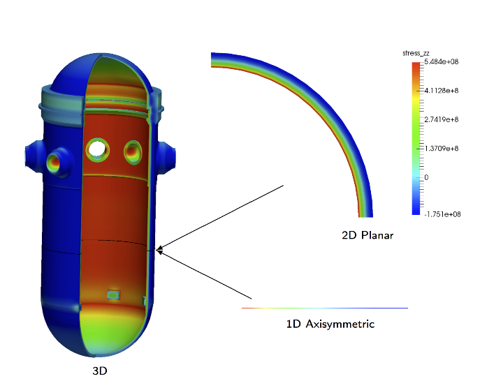
Figure 1: 1D, 2D, and 3D Grizzly models of the global RPV response.
Computational Model Description
This model uses quarter symmetry to represent the coupled thermal/mechanical response of an RPV subjected to transient loading. The geometry and loading conditions are representative of those that would be observed in an actual PWR RPV. Figure 2 shows the mesh of this quarter-symmetry model, which includes an inlet and outlet, and represents the entire RPV quadrant.
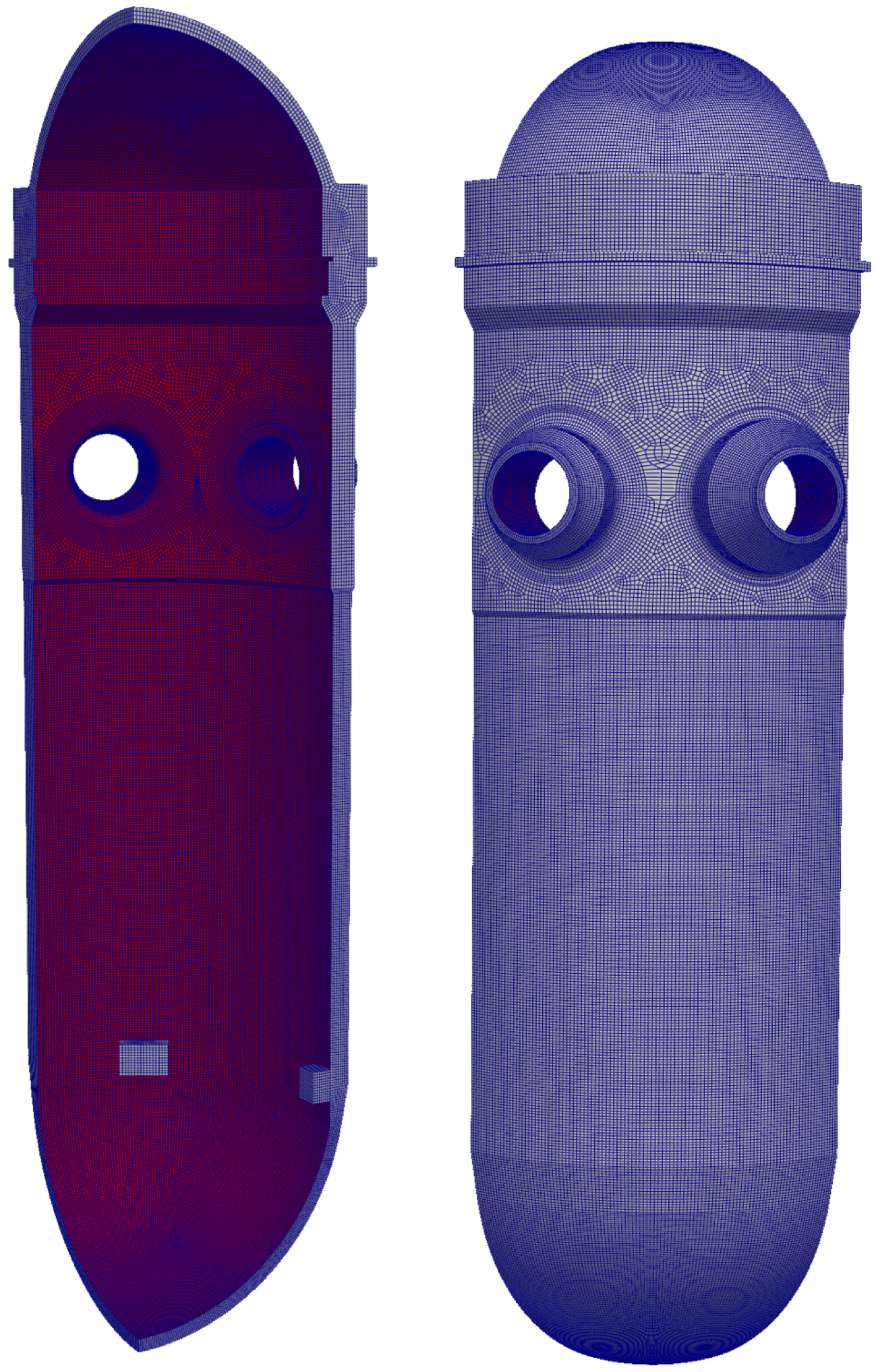
Figure 2: 3D Mesh of RPV used for this case, shown from the interior (left) and exterior (right)
Files used by this model include:
MOOSE input file
Exodus mesh file
CSV (comma-separated value) file defining the time history of the pressure
CSV file defining the time history of the coolant temperature
CSV file defining the time history of the heat transfer coefficient
This document reviews the basic elements of the input file, listed in full here:
# ==============================================================================
# 3D Thermo-mechanical analysis of Light Water Reactor Pressure Vessel
# Application : Grizzly
# ------------------------------------------------------------------------------
# Idaho Falls, INL, 2024
# Author(s): Ben Spencer, Will Hoffman
# If using or referring to this model, please cite as explained on
# https://mooseframework.inl.gov/virtual_test_bed/citing.html
# ==============================================================================

[GlobalParams]
  order = FIRST
  family = LAGRANGE
  displacements = 'disp_x disp_y disp_z'
[]

[Mesh]
  file = rpv_fine.e
  use_displaced_mesh = false
[]

[Problem]
  type = ReferenceResidualProblem
  extra_tag_vectors = 'ref'
  reference_vector = 'ref'
  group_variables = 'disp_x disp_y disp_z'
[]

[Variables]
  [temp]
    initial_condition = 559.23333
  []
[]

[AuxVariables]
  [hoop_stress_clad]
    order = FIRST
    family = MONOMIAL
  []
  [axial_stress_clad]
    order = FIRST
    family = MONOMIAL
  []
  [hoop_stress_base]
    order = FIRST
    family = MONOMIAL
  []
  [axial_stress_base]
    order = FIRST
    family = MONOMIAL
  []
[]

[Physics/SolidMechanics/QuasiStatic]
  [all]
    strain = SMALL
    temperature = temp
    add_variables = true
    generate_output = 'stress_xx stress_yy stress_zz'
    eigenstrain_names = thermal_eigenstrain
    extra_vector_tags = 'ref'
  []
[]

[Kernels]
  [heat]
    type = HeatConduction
    variable = temp
    extra_vector_tags = 'ref'
  []
  [heat_ie]
    type = HeatConductionTimeDerivative
    variable = temp
    extra_vector_tags = 'ref'
  []
[]

[AuxKernels]
  [axial_stress_clad]
    type = MaterialRealAux
    block = 2
    property = axial_stress_clad
    variable = axial_stress_clad
  []
  [hoop_stress_clad]
    type = MaterialRealAux
    block = 2
    property = hoop_stress_clad
    variable = hoop_stress_clad
  []
  [axial_stress_base]
    type = MaterialRealAux
    block = 1
    property = axial_stress_base
    variable = axial_stress_base
  []
  [hoop_stress_base]
    type = MaterialRealAux
    block = 1
    property = hoop_stress_base
    variable = hoop_stress_base
  []
[]

[Functions]
  [time_steps]
    type = PiecewiseLinear
    xy_data = '0 1
               1 59
               60 60'
  []
  [coolant_pressure_history]
    type = PiecewiseLinear
    data_file = pressure_history.csv
    format = columns
  []
  [coolant_temperature_history]
    type = PiecewiseLinear
    data_file = temperature_history.csv
    format = columns
  []
  [heat_transfer_coefficient_history]
    type = PiecewiseLinear
    data_file = heat_transfer_coefficient_history.csv
    format = columns
  []
  [cte_func_clad]
    type = PiecewiseLinear
    x = '294.26 310.93 338.71 366.48 394.26 422.04 449.82 477.59 505.37 533.15 560.93 588.71 616.48 644.26 672.04 699.82'
    y = '8.50e-6 8.70e-6 9.00e-6 9.40e-6 9.60e-6 9.90e-6 1.01e-5 1.02e-5 1.04e-5 1.05e-5 1.06e-5 1.06e-5 1.07e-5 1.08e-5 1.08e-5 1.09e-5'
    scale_factor = 1.8
  []
  [cte_func_base]
    type = PiecewiseLinear
    x = '294.26 310.93 338.71 366.48 394.26 422.04 449.82 477.59 505.37 533.15 560.93 588.71 616.48 644.26'
    y = '6.40e-6 6.60e-6 6.80e-6 7.00e-6 7.20e-6 7.30e-6 7.50e-6 7.70e-6 7.80e-6 8.00e-6 8.20e-6 8.30e-6 8.50e-6 8.70e-6'
    scale_factor = 1.8
  []
  [k_func_clad]
    type = PiecewiseLinear
    x = '294.26 310.93 338.71 366.48 394.26 422.04 449.82 477.59 505.37 533.15 560.93 588.71 616.48 644.26 672.04 699.82'
    y = '8.6 8.7 9.0 9.3 9.6 9.8 10.1 10.4 10.6 10.9 11.1 11.3 11.6 11.8 12.0 12.3'
    scale_factor = 1.73
  []
  [k_func_base]
    type = PiecewiseLinear
    x = '294.26 310.93 338.71 366.48 394.26 422.04 449.82 477.59 505.37 533.15 560.93 588.71 616.48 644.26 672.04 699.82'
    y = '23.7 23.6 23.5 23.5 23.4 23.4 23.3 23.1 23.0 22.7 22.5 22.2 21.9 21.6 21.3 21.0'
    scale_factor = 1.73
  []
  [c_func_clad]
    type = PiecewiseLinear
    x = '294.26 310.93 338.71 366.48 394.26 422.04 449.82 477.59 505.37 533.15 560.93 588.71 616.48 644.26 672.04 699.82'
    y = '0.118 0.118 0.121 0.123 0.126 0.127 0.129 0.130 0.131 0.133 0.133 0.134 0.135 0.136 0.136 0.138'
    scale_factor = 4186.8
  []
  [c_func_base]
    type = PiecewiseLinear
    x = '294.26 310.93 338.71 366.48 394.26 422.04 449.82 477.59 505.37 533.15 560.93 588.71 616.48 644.26 672.04 699.82'
    y = '0.107 0.108 0.111 0.115 0.117 0.121 0.123 0.126 0.129 0.131 0.134 0.137 0.139 0.142 0.145 0.149'
    scale_factor = 4186.8
  []
[]

[BCs]
  [no_x_all]
    type = DirichletBC
    variable = disp_x
    boundary = '1'
    value = 0.0
  []

  [no_y_all]
    type = DirichletBC
    variable = disp_y
    boundary = '2'
    value = 0.0
  []
  [no_z]
    type = DirichletBC
    variable = disp_z
    boundary = '101'
    value = 0.0
  []

  [Pressure]
    [coolantPressure]
      boundary = 3
      factor = 1e6
      function = coolant_pressure_history
    []
  []
  [convective_flux_inner_surface]
    type = ConvectiveFluxFunction
    boundary = 3
    variable = temp
    coefficient = heat_transfer_coefficient_history
    T_infinity = coolant_temperature_history
  []
[]

[Materials]
  [thermal_base]
    type = HeatConductionMaterial
    block = '1'
    thermal_conductivity_temperature_function = k_func_base
    specific_heat_temperature_function = c_func_base
    temp = temp
  []

  [thermal_clad]
    type = HeatConductionMaterial
    block = '2'
    thermal_conductivity_temperature_function = k_func_clad
    specific_heat_temperature_function = c_func_clad
    temp = temp
  []

  [youngs_modulus_base]
    type = PiecewiseLinearInterpolationMaterial
    x = '294.26 366.48 422.04 477.59 533.15 588.71 644.26'
    y = '27.8e6 27.1e6 26.7e6 26.2e6 25.7e6 25.1e6 24.6e6'
    scale_factor = 6894.7573
    property = youngs_modulus_base
    variable = temp
    block = 1
  []
  [elastic_tensor_base]
    type = ComputeVariableIsotropicElasticityTensor
    args = temp
    youngs_modulus = youngs_modulus_base
    poissons_ratio = 0.3
    block = 1
  []
  [stress_base]
    type = ComputeLinearElasticStress
    block = 1
  []
  [thermal_strain_base]
    type = ComputeMeanThermalExpansionFunctionEigenstrain
    temperature = temp
    thermal_expansion_function = cte_func_base
    thermal_expansion_function_reference_temperature = 294.26111
    stress_free_temperature = 526.4833
    eigenstrain_name = thermal_eigenstrain
    block = 1
  []

  [youngs_modulus_clad]
    type = PiecewiseLinearInterpolationMaterial
    x = '294.26 366.48 422.04 477.59 533.15 588.71 644.26'
    y = '28.3e6 27.5e6 27.0e6 26.4e6 25.9e6 25.3e6 24.8e6'
    scale_factor = 6894.7573
    property = youngs_modulus_clad
    variable = temp
    block = 2
  []
  [elastic_tensor_clad]
    type = ComputeVariableIsotropicElasticityTensor
    args = temp
    youngs_modulus = youngs_modulus_clad
    poissons_ratio = 0.31
    block = 2
  []
  [stress_clad]
    type = ComputeLinearElasticStress
    block = 2
  []
  [thermal_strain_clad]
    type = ComputeMeanThermalExpansionFunctionEigenstrain
    temperature = temp
    thermal_expansion_function = cte_func_clad
    thermal_expansion_function_reference_temperature = 294.26111
    stress_free_temperature = 526.4833
    eigenstrain_name = thermal_eigenstrain
    block = 2
  []

  [density_base]
    type = Density
    block = '1'
    density = 7750.4
  []

  [density_clad]
    type = Density
    block = '2'
    density = 8027.2
  []

  [axial_stress_clad]
    type = RankTwoCylindricalComponent
    block = 2
    rank_two_tensor = stress
    property_name = axial_stress_clad
    cylindrical_component = AxialStress
    cylindrical_axis_point1 = '0. 0. 0.'
    cylindrical_axis_point2 = '0. 0. 1.'
  []
  [hoop_stress_clad]
    type = RankTwoCylindricalComponent
    block = 2
    rank_two_tensor = stress
    cylindrical_component = HoopStress
    property_name = hoop_stress_clad
    cylindrical_axis_point1 = '0. 0. 0.'
    cylindrical_axis_point2 = '0. 0. 1.'
  []
  [axial_stress_base]
    type = RankTwoCylindricalComponent
    block = 1
    rank_two_tensor = stress
    cylindrical_component = AxialStress
    property_name = axial_stress_base
    cylindrical_axis_point1 = '0. 0. 0.'
    cylindrical_axis_point2 = '0. 0. 1.'
  []
  [hoop_stress_base]
    type = RankTwoCylindricalComponent
    block = 1
    rank_two_tensor = stress
    cylindrical_component = HoopStress
    property_name = hoop_stress_base
    cylindrical_axis_point1 = '0. 0. 0.'
    cylindrical_axis_point2 = '0. 0. 1.'
  []
[]

[Preconditioning]
  [SMP]
    type = SMP
    full = true
  []
[]

[Dampers]
  [limit_temp]
    type = MaxIncrement
    max_increment = 50.0
    variable = temp
  []
[]

[Executioner]
  automatic_scaling = true
  solve_type = 'PJFNK'
  type = Transient
  petsc_options = '-snes_ksp_ew'
  petsc_options_iname = '-ksp_gmres_restart -pc_type -pc_hypre_type -pc_hypre_boomeramg_max_iter -pc_hypre_boomeramg_strong_threshold'
  petsc_options_value = ' 201                hypre    boomeramg      4                           0.6'

  l_max_its = 25
  nl_max_its = 50
  nl_rel_tol = 1e-8
  nl_abs_tol = 1e-11

  start_time = 0.0
  dt = 1
  end_time = 2000

  [Predictor]
    type = SimplePredictor
    scale = 1.0
    skip_times_old = '1'
  []

  dtmax = 60
  dtmin = 1

  [TimeStepper]
    type = FunctionDT
    function = time_steps
  []
[]

[LineSamplers]
  total_thickness = 0.219202
  clad_thickness = 0.004064
  inner_radius = 2.1971
  base_block = 1
  clad_block = 2
  coord_system = 3D_CARTESIAN
  axis_of_rotation = z
  line_sampler_type = LineValueSampler
  temperature = 'temp'
  axial_stress_base = axial_stress_base
  hoop_stress_base = hoop_stress_base
  axial_stress_clad = axial_stress_clad
  hoop_stress_clad = hoop_stress_clad
  base_order = 4
  axial_start = -0.2
  axial_end = 4.2
  axial_num_points = 16
  azimuthal_start = 0
  azimuthal_end = 90
  azimuthal_num_points = 12
  azimuth0 = '1 0 0'
  base_thickness_offset_fraction = 0.01
  clad_thickness_offset_fraction = 0.01
[]

[Outputs]
  wall_time_checkpoint = false
  exodus = true
  perf_graph = true
  csv = true
[]GlobalParams
This block contains parameters that are applied automatically in any context where they are applicable in the rest of the model. A few important things are defined here:
The
ORDERandFAMILYparameters are used to define the interpolation order and type of interpolation, and are used for multiple types of variables. The parameters here give 1st order variables, which are appropriate for the linear eight-noded hexahedral elements used in the mesh.The
displacementsparameter defines the set of displacement variables, which is used in multiple mechanics models.
[GlobalParams]
  order = FIRST
  family = LAGRANGE
  displacements = 'disp_x disp_y disp_z'
[]Mesh
This block defines the finite element mesh that will be used. In this case, the mesh is read from a file in the Exodus (.e) format. The mesh for this particular problem was created using Cubit.
[Mesh]
  file = rpv_fine.e
  use_displaced_mesh = false
[]Problem
This block is used to define parameters for the ReferenceResidualProblem, which is defined to override the standard MOOSE convergence checks and ensure that the individual variables are converged relative to meaningful values. All parameters in this block in this example are specifically related to controlling those convergence checks.
[Problem]
  type = ReferenceResidualProblem
  extra_tag_vectors = 'ref'
  reference_vector = 'ref'
  group_variables = 'disp_x disp_y disp_z'
[]Variables
This block defines the field variables that will be solved for in the nonlinear equation system. In this model, the only variable defined in this step is the temperature.
The temperature (
temp) is set to have an initial condition equal to the coolant temperature during operation (in Kelvin).
The model also solves for the mechnical displacement fields, but these are set up automatically via the Physics/SolidMechanics/QuasiStatic block.
[Variables]
  [temp]
    initial_condition = 559.23333
  []
[]AuxVariables
This block defines AuxVariables (i.e., auxiliary variables), which are field variables that are not part of the system of equations being solved. In this case, these are all for output of stress components. It should be noted that output for some of the stress component outputs is handled automatically in the Physics/SolidMechanics/QuasiStatic block, but the AuxVariables are manually created because special options are used to preserve the discontinuity in the stress between the base metal and cladding.
[AuxVariables]
  [hoop_stress_clad]
    order = FIRST
    family = MONOMIAL
  []
  [axial_stress_clad]
    order = FIRST
    family = MONOMIAL
  []
  [hoop_stress_base]
    order = FIRST
    family = MONOMIAL
  []
  [axial_stress_base]
    order = FIRST
    family = MONOMIAL
  []
[]Physics/SolidMechanics/QuasiStatic
This block automates the process of setting up multiple objects related to solution of a mechanics problem. The objects set up by this block include the Variables and Kernels for the displacement solution, the Material that computes the strain, and objects associated with outputing stresses. In addition to simplifying the input, this ensures that a consistent set of options are selected for the desired formulation.
[Physics]
  [SolidMechanics]
    [QuasiStatic]
      [all]
        strain = SMALL
        temperature = temp
        add_variables = true
        generate_output = 'stress_xx stress_yy stress_zz'
        eigenstrain_names = thermal_eigenstrain
        extra_vector_tags = 'ref'
      []
    []
  []
[]Kernels
This block defines the terms in the partial differential equations for the physics being modeled. In this case, the temperature and displacements are being solved for, but only blocks applicable for the temperature variable appear here because those applicable to the mechanics solution are set up automatically by the Physics/SolidMechanics/QuasiStatic block.
[Kernels]
  [heat]
    type = HeatConduction
    variable = temp
    extra_vector_tags = 'ref'
  []
  [heat_ie]
    type = HeatConductionTimeDerivative
    variable = temp
    extra_vector_tags = 'ref'
  []
[]AuxKernels
This block defines the models that compute the values stored in the AuxVariables that were previously defined. In this case, these are objects that extract components of the stress tensor and make them available as field variables.
[AuxKernels]
  [axial_stress_clad]
    type = MaterialRealAux
    block = 2
    property = axial_stress_clad
    variable = axial_stress_clad
  []
  [hoop_stress_clad]
    type = MaterialRealAux
    block = 2
    property = hoop_stress_clad
    variable = hoop_stress_clad
  []
  [axial_stress_base]
    type = MaterialRealAux
    block = 1
    property = axial_stress_base
    variable = axial_stress_base
  []
  [hoop_stress_base]
    type = MaterialRealAux
    block = 1
    property = hoop_stress_base
    variable = hoop_stress_base
  []
[]Functions
This block defines functions, which are used to define various properties that can be a function of time and space, or a function of a variable like temperature. These are all used elsewhere in the model, and are referred to by their names. Several types of functions are used here:
A function called
time_stepsis used to define the time step size as a function of the solution time.Three functions are used to define the time history of the coolant pressure, coolant temperature, and heat transfer coefficient. These are all read in from external CSV files. These functions were designed to loosely resemble a scenario in which a coolant valve is opened and closed during operation. Thus the transient begins with a rapid depressurization and cool down, followed by a period of repressurization and temperature increase. This transient was created as a demonstration only and does not represent actual expected reactor conditions.
Functions are used to define the coefficient of thermal expansion, thermal conductivity, and specific heat of the steels used for the base metal and cladding. These functions are defined in terms of temperature and are used by material models that refer to them.
[Functions]
  [time_steps]
    type = PiecewiseLinear
    xy_data = '0 1
               1 59
               60 60'
  []
  [coolant_pressure_history]
    type = PiecewiseLinear
    data_file = pressure_history.csv
    format = columns
  []
  [coolant_temperature_history]
    type = PiecewiseLinear
    data_file = temperature_history.csv
    format = columns
  []
  [heat_transfer_coefficient_history]
    type = PiecewiseLinear
    data_file = heat_transfer_coefficient_history.csv
    format = columns
  []
  [cte_func_clad]
    type = PiecewiseLinear
    x = '294.26 310.93 338.71 366.48 394.26 422.04 449.82 477.59 505.37 533.15 560.93 588.71 616.48 644.26 672.04 699.82'
    y = '8.50e-6 8.70e-6 9.00e-6 9.40e-6 9.60e-6 9.90e-6 1.01e-5 1.02e-5 1.04e-5 1.05e-5 1.06e-5 1.06e-5 1.07e-5 1.08e-5 1.08e-5 1.09e-5'
    scale_factor = 1.8
  []
  [cte_func_base]
    type = PiecewiseLinear
    x = '294.26 310.93 338.71 366.48 394.26 422.04 449.82 477.59 505.37 533.15 560.93 588.71 616.48 644.26'
    y = '6.40e-6 6.60e-6 6.80e-6 7.00e-6 7.20e-6 7.30e-6 7.50e-6 7.70e-6 7.80e-6 8.00e-6 8.20e-6 8.30e-6 8.50e-6 8.70e-6'
    scale_factor = 1.8
  []
  [k_func_clad]
    type = PiecewiseLinear
    x = '294.26 310.93 338.71 366.48 394.26 422.04 449.82 477.59 505.37 533.15 560.93 588.71 616.48 644.26 672.04 699.82'
    y = '8.6 8.7 9.0 9.3 9.6 9.8 10.1 10.4 10.6 10.9 11.1 11.3 11.6 11.8 12.0 12.3'
    scale_factor = 1.73
  []
  [k_func_base]
    type = PiecewiseLinear
    x = '294.26 310.93 338.71 366.48 394.26 422.04 449.82 477.59 505.37 533.15 560.93 588.71 616.48 644.26 672.04 699.82'
    y = '23.7 23.6 23.5 23.5 23.4 23.4 23.3 23.1 23.0 22.7 22.5 22.2 21.9 21.6 21.3 21.0'
    scale_factor = 1.73
  []
  [c_func_clad]
    type = PiecewiseLinear
    x = '294.26 310.93 338.71 366.48 394.26 422.04 449.82 477.59 505.37 533.15 560.93 588.71 616.48 644.26 672.04 699.82'
    y = '0.118 0.118 0.121 0.123 0.126 0.127 0.129 0.130 0.131 0.133 0.133 0.134 0.135 0.136 0.136 0.138'
    scale_factor = 4186.8
  []
  [c_func_base]
    type = PiecewiseLinear
    x = '294.26 310.93 338.71 366.48 394.26 422.04 449.82 477.59 505.37 533.15 560.93 588.71 616.48 644.26 672.04 699.82'
    y = '0.107 0.108 0.111 0.115 0.117 0.121 0.123 0.126 0.129 0.131 0.134 0.137 0.139 0.142 0.145 0.149'
    scale_factor = 4186.8
  []
[]BCs
As previously stated, this model uses quarter symmetry to minimize computational resources. Dirichlet boundary conditions fixing the x and y displacements on the appropriate symmetry planes are imposed. To prevent rigid-body translation, the z displacement is fixed at the bottom node of the model, which coincides with the axis of rotation.
The pressure and temperature boundary conditions are also applied in this block. The applied pressure acts on the displacement variables defined in the Global Parameters block, and a convective flux boundary condition acts on the temperature variable. These both rely on functions defined in the Functions block and are applied to the inner surface of the RPV.
[BCs]
  [no_x_all]
    type = DirichletBC
    variable = disp_x
    boundary = '1'
    value = 0.0
  []

  [no_y_all]
    type = DirichletBC
    variable = disp_y
    boundary = '2'
    value = 0.0
  []
  [no_z]
    type = DirichletBC
    variable = disp_z
    boundary = '101'
    value = 0.0
  []

  [Pressure]
    [coolantPressure]
      boundary = 3
      factor = 1e6
      function = coolant_pressure_history
    []
  []
  [convective_flux_inner_surface]
    type = ConvectiveFluxFunction
    boundary = 3
    variable = temp
    coefficient = heat_transfer_coefficient_history
    T_infinity = coolant_temperature_history
  []
[]Materials
This block is used to define the thermal and mechanical properties for the base and cladding material. The thermal models use temperature-dependent functions for the thermal conductivity and specific heat, using functions defined in the Functions block.
The mechanical properties are also temperature-dependent. The temperature-dependent Young's modulus is defined using a generic material model that defines a property as a function of a variable, using a piecewise linear interpolation defined within the material block. The temperature-dependent thermal expansion is defined using a model that refers to a function defined in the Functions block.
[Materials]
  [thermal_base]
    type = HeatConductionMaterial
    block = '1'
    thermal_conductivity_temperature_function = k_func_base
    specific_heat_temperature_function = c_func_base
    temp = temp
  []

  [thermal_clad]
    type = HeatConductionMaterial
    block = '2'
    thermal_conductivity_temperature_function = k_func_clad
    specific_heat_temperature_function = c_func_clad
    temp = temp
  []

  [youngs_modulus_base]
    type = PiecewiseLinearInterpolationMaterial
    x = '294.26 366.48 422.04 477.59 533.15 588.71 644.26'
    y = '27.8e6 27.1e6 26.7e6 26.2e6 25.7e6 25.1e6 24.6e6'
    scale_factor = 6894.7573
    property = youngs_modulus_base
    variable = temp
    block = 1
  []
  [elastic_tensor_base]
    type = ComputeVariableIsotropicElasticityTensor
    args = temp
    youngs_modulus = youngs_modulus_base
    poissons_ratio = 0.3
    block = 1
  []
  [stress_base]
    type = ComputeLinearElasticStress
    block = 1
  []
  [thermal_strain_base]
    type = ComputeMeanThermalExpansionFunctionEigenstrain
    temperature = temp
    thermal_expansion_function = cte_func_base
    thermal_expansion_function_reference_temperature = 294.26111
    stress_free_temperature = 526.4833
    eigenstrain_name = thermal_eigenstrain
    block = 1
  []

  [youngs_modulus_clad]
    type = PiecewiseLinearInterpolationMaterial
    x = '294.26 366.48 422.04 477.59 533.15 588.71 644.26'
    y = '28.3e6 27.5e6 27.0e6 26.4e6 25.9e6 25.3e6 24.8e6'
    scale_factor = 6894.7573
    property = youngs_modulus_clad
    variable = temp
    block = 2
  []
  [elastic_tensor_clad]
    type = ComputeVariableIsotropicElasticityTensor
    args = temp
    youngs_modulus = youngs_modulus_clad
    poissons_ratio = 0.31
    block = 2
  []
  [stress_clad]
    type = ComputeLinearElasticStress
    block = 2
  []
  [thermal_strain_clad]
    type = ComputeMeanThermalExpansionFunctionEigenstrain
    temperature = temp
    thermal_expansion_function = cte_func_clad
    thermal_expansion_function_reference_temperature = 294.26111
    stress_free_temperature = 526.4833
    eigenstrain_name = thermal_eigenstrain
    block = 2
  []

  [density_base]
    type = Density
    block = '1'
    density = 7750.4
  []

  [density_clad]
    type = Density
    block = '2'
    density = 8027.2
  []

  [axial_stress_clad]
    type = RankTwoCylindricalComponent
    block = 2
    rank_two_tensor = stress
    property_name = axial_stress_clad
    cylindrical_component = AxialStress
    cylindrical_axis_point1 = '0. 0. 0.'
    cylindrical_axis_point2 = '0. 0. 1.'
  []
  [hoop_stress_clad]
    type = RankTwoCylindricalComponent
    block = 2
    rank_two_tensor = stress
    cylindrical_component = HoopStress
    property_name = hoop_stress_clad
    cylindrical_axis_point1 = '0. 0. 0.'
    cylindrical_axis_point2 = '0. 0. 1.'
  []
  [axial_stress_base]
    type = RankTwoCylindricalComponent
    block = 1
    rank_two_tensor = stress
    cylindrical_component = AxialStress
    property_name = axial_stress_base
    cylindrical_axis_point1 = '0. 0. 0.'
    cylindrical_axis_point2 = '0. 0. 1.'
  []
  [hoop_stress_base]
    type = RankTwoCylindricalComponent
    block = 1
    rank_two_tensor = stress
    cylindrical_component = HoopStress
    property_name = hoop_stress_base
    cylindrical_axis_point1 = '0. 0. 0.'
    cylindrical_axis_point2 = '0. 0. 1.'
  []
[]Preconditioning
This block is used to request that a full matrix with all coupling terms between variables be constructed. This provides a more efficient solution of this particular problem.
[Preconditioning]
  [SMP]
    type = SMP
    full = true
  []
[]Dampers
This block is used to limit the change in the temperature solution during each nonlinear iteration, which improves the robustness of the solution by keeping the temperature within acceptable limits. Using a damper can result in a higher number of iterations in some steps when there are significant changes to the solution, but the robustness benefits outweigh the additional computational expense from the additional iterations.
[Dampers]
  [limit_temp]
    type = MaxIncrement
    max_increment = 50.0
    variable = temp
  []
[]Executioner
The parameters in this block control the solution strategy used, convergence tolerances, start and end time, and the use of a predictor, which accelerates convergence when loading is mostly monotonic in nature.
[Executioner]
  automatic_scaling = true
  solve_type = 'PJFNK'
  type = Transient
  petsc_options = '-snes_ksp_ew'
  petsc_options_iname = '-ksp_gmres_restart -pc_type -pc_hypre_type -pc_hypre_boomeramg_max_iter -pc_hypre_boomeramg_strong_threshold'
  petsc_options_value = ' 201                hypre    boomeramg      4                           0.6'

  l_max_its = 25
  nl_max_its = 50
  nl_rel_tol = 1e-8
  nl_abs_tol = 1e-11

  start_time = 0.0
  dt = 1
  end_time = 2000

  [Predictor]
    type = SimplePredictor
    scale = 1.0
    skip_times_old = '1'
  []

  dtmax = 60
  dtmin = 1

  [TimeStepper]
    type = FunctionDT
    function = time_steps
  []
[]LineSamplers
This block defines a MOOSE Action that automates the process of setting up the line samplers, which sample values along lines through the cladding and base metal and fit those values to polynomial coefficients. These are used in the PFM simulation, which computes stress intensity factors for flaws at a variety of locations. For a 3D RPV model such as this, a grid of lines is set up spanning the region specified by the axial and azimuthal start and end points. Sampling is done along each line through the thickness of the RPV. The PFM calculation interpolates between those values.
[LineSamplers]
  total_thickness = 0.219202
  clad_thickness = 0.004064
  inner_radius = 2.1971
  base_block = 1
  clad_block = 2
  coord_system = 3D_CARTESIAN
  axis_of_rotation = z
  line_sampler_type = LineValueSampler
  temperature = 'temp'
  axial_stress_base = axial_stress_base
  hoop_stress_base = hoop_stress_base
  axial_stress_clad = axial_stress_clad
  hoop_stress_clad = hoop_stress_clad
  base_order = 4
  axial_start = -0.2
  axial_end = 4.2
  axial_num_points = 16
  azimuthal_start = 0
  azimuthal_end = 90
  azimuthal_num_points = 12
  azimuth0 = '1 0 0'
  base_thickness_offset_fraction = 0.01
  clad_thickness_offset_fraction = 0.01
[]Outputs
This block defines the types of output that are generated. It is essential to ask for CSV output in order to obtain the line samples, which are used in a subsequent PFM analysis. The Exodus output is primarily used for inspection of the results.
[Outputs]
  wall_time_checkpoint = false
  exodus = true
  perf_graph = true
  csv = true
[]Running the model
To run this model using the Grizzly executable, run the following command:
mpiexec -n 16 /path/to/app/grizzly-opt -i rpv_thermomechanical_3d.i
This model is large and will take hours to run. The use of multiple processors is highly recommended for a model of this size, and the number of processors is specifed using the -n option in the mpiexec command. Using 36 processors it takes approximately 5 hours to run to completion. The following output files will be produced:
The Exodus results file:
rpv_thermomechanical_3d_out.eA set of CSV files with time histories of the stress coefficients for use in PFM analysis. These have names starting with
rpv_thermomechanical_3d_out_coefs_.
The Exodus output file can be visualized with Paraview.
References
- E. Cohn, P. Raynaud, S. E. Veras, C. Nellis, and C. Ulmer.
FAVPRO v1.0 user's manual.
Technical Report TLR-RES/DE/REB-2024-07, United States Nuclear Regulatory Commission, Washington, DC, June 2024.
URL: https://www.nrc.gov/docs/ML2411/ML24113A237.pdf.[BibTeX]
- Guian Qian and Markus Niffenegger.
Procedures, methods and computer codes for the probabilistic assessment of reactor pressure vessels subjected to pressurized thermal shocks.
Nuclear Engineering and Design, 258:35–50, May 2013.
doi:10.1016/j.nucengdes.2013.01.030.[BibTeX]
- B.W. Spencer, W.M. Hoffman, and M.A. Backman.
Modular system for probabilistic fracture mechanics analysis of embrittled reactor pressure vessels in the Grizzly code.
Nuclear Engineering and Design, 341:25–37, January 2019.
doi:10.1016/j.nucengdes.2018.10.015.[BibTeX]
- Benjamin W. Spencer, William M. Hoffman, Sudipta Biswas, Wen Jiang, Alain Giorla, and Marie A. Backman.
Grizzly and BlackBear: structural component aging simulation codes.
Nuclear Technology, 207(7):981–1003, April 2021.
doi:10.1080/00295450.2020.1868278.[BibTeX]