Nek5000/RS CFD Modeling of HTTF Lower Plenum Flow Mixing Phenomenon

Contact: Jun Fang, fangj.at.anl.gov

Model link: HTTF Lower Plenum CFD Model

Overview

Accurate modeling and simulation capabilities are becoming increasingly important to speed up the development and deployment of advanced nuclear reactor technologies, such as high temperature gas-cooled reactors. Among the identified safety-relevant phenomena for the gas-cooled reactors (GCR), the outlet plenum flow distribution was ranked to be of high importance with a low knowledge level in the phenomenon identification and ranking table (PIRT) (Ball et al., 2008). The heated coolant (e.g., helium) flows downward through the GCR core region and enters the outlet/lower plenum through narrow channels, which causes the jetting of the gas flow. The jets have a non-uniform temperature and risk yielding high cycling thermal stresses in the lower plenum, negative pressure gradients opposing the flow ingress, and hot streaking. These phenomena cannot be accurately captured by 1-D system codes; instead, the modeling requires using higher fidelity CFD codes that can predict the temperature fluctuations in the HTTF lower plenum. In this study, a detailed CFD model is established for the lower plenum of scaled, electrically-heated GCR test facility (i.e., High Temperature Test Facility, or HTTF) at Oregon State University. Specifically, the flow mixing phenomenon in HTTF lower plenum is simulated with spectral element CFD software, Nek5000 and its GPU-oriented variant nekRS. The turbulence effects are modeled by the two-equation $var element = document.getElementById("moose-equation-398c3214-b193-43d3-9b54-ec697ade7436");katex.render("k-\\tau", element, {displayMode:false,throwOnError:false});$ URANS model. Two sets of boundary conditions are studied in the Nek5000 and nekRS simulations, respectively. The velocity and temperature fields are examined to understand the thermal-fluid physics happening during the lower plenum mixing. As part of the HTTF international benchmark campaign, the simulation results generated from this study will be used for code-to-code and code-to-data comparisons in the near future, which would lay a solid foundation for the use of CFD in GCR research and development.

note

This documentation assumes that the reader has basic knowledge of Nek5000, and is able to run the example cases provided in the Nek5000 tutorial. The specific Nek5000 version used here is v19.0. Although Nek5000 input files are not tested regularly in the Moose CI test suite, Nek5000 does offer reliable backward compatibility. No foreseeable compatibility issues are expected. In rare situations where there is indeed a compatibility issue, please reach out to the Nek5000 developer team via Nek5000 Google Group. Meanwhile, nekRS code is still under active development, and there is only a beta version of nekRS online tutorial.

Geometry and Meshing

The HTTF lower plenum (i.e., core outlet plenum) geometry is illustrated in Figure 1, which contains 163 ceramic cylindrical posts on which the core structure stands. It is enclosed by lower side reflectors, lower plenum floor and lower plenum roof. The height of the lower plenum is 22.2 $var element = document.getElementById("moose-equation-51ec5355-3e5b-4ecd-883f-9f5c29088afe");katex.render("cm", element, {displayMode:false,throwOnError:false});$ . Helium gas enters the lower plenum through core coolant channels and exits through the horizontal hot duct. There are 234 inlet channels with the same diameter of 1 $var element = document.getElementById("moose-equation-0071301c-6af3-4e99-9b77-357f21748c74");katex.render("in", element, {displayMode:false,throwOnError:false});$ (i.e., 2.54 $var element = document.getElementById("moose-equation-58b75532-7db1-4673-bf8f-60681114fc86");katex.render("cm", element, {displayMode:false,throwOnError:false});$ ). A cylindrical hot duct is connected to the lower plenum, which functions as the outlet channel. Rakes are installed in the hot duct to house measurement instruments in the experiments.

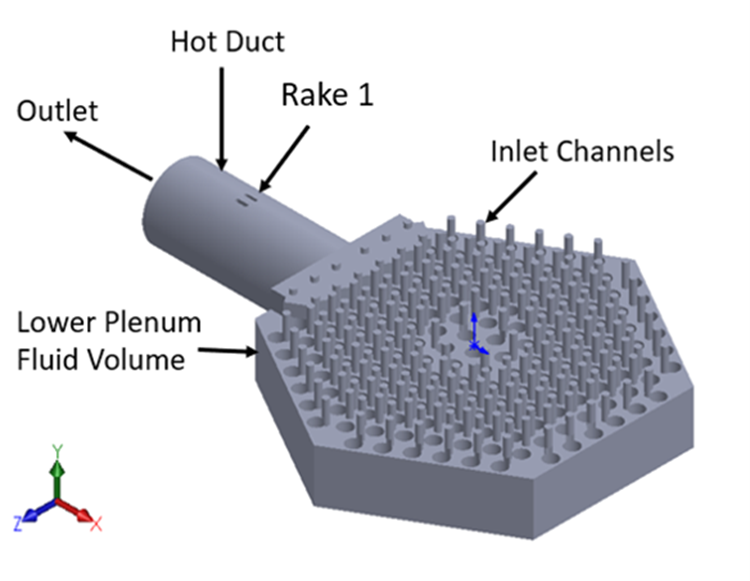
Figure 1: Overview of the HTTF lower plenum geometry.

Nek5000/RS requires a pure hexahedral mesh to perform the calculations. Due to the domain complexity, it is challenging to create an unstructured mesh with only hexahedral cells. A two-step approach is adopted in the meshing practice. We first used the commercial software, ANSYS Mesh, to generate an unstructured computational mesh consisting of tetrahedra cells (in the bulk) and wedge cells (in the boundary layer region), and then converted it into a pure hexahedra mesh using a native quadratic tet-to-hex utility. To ensure the accuracy of wall-resolved RANS calculations, the first layer of grid points off the wall is kept at a distance of $var element = document.getElementById("moose-equation-6d29cf8d-065f-4380-a59c-1253645ac203");katex.render("y^+ < 1.0", element, {displayMode:false,throwOnError:false});$ . As shown in Figure 2, the resulting mesh has 2.60 million cells, and the total degrees of freedom is approximately 72.86 million in Nek5000 simulations with a polynomial order of 3. Note that the polynomial order is kept relatively low to limit the computational costs. It can be readily increased for higher-fidelity simulations, such as a Large Eddy Simulation (LES), given necessary computing hours.

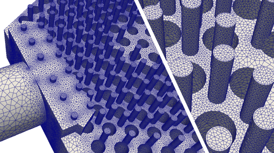
Figure 2: The hexahedral mesh of HTTF lower plenum from the tet-to-hex conversion.

Nek5000 Investigation

Boundary conditions

The boundary conditions adopted in the Nek5000 simulations are taken from the corresponding system modeling of HTTF system using RELAP5-3D (Halsted, 2022). The 234 inlet channels are divided into five rings as shown in Figure 3 based on the radial locations, and each ring with specific mass flow rate and temperature. Inside the lower plenum (LP), the floor, roof, posts and side reflector walls all have distinct temperature values. The LP roof has the highest temperature while the side walls sees the lowest. Details of the thermal boundary conditions are listed in Table 1. Inlet channels within a specific ring are assumed to have fixed inflow velocity according to the mass flow rate, and the no-slip condition is imposed to all wall surfaces. A natural pressure condition is given to the outlet face of hot duct.

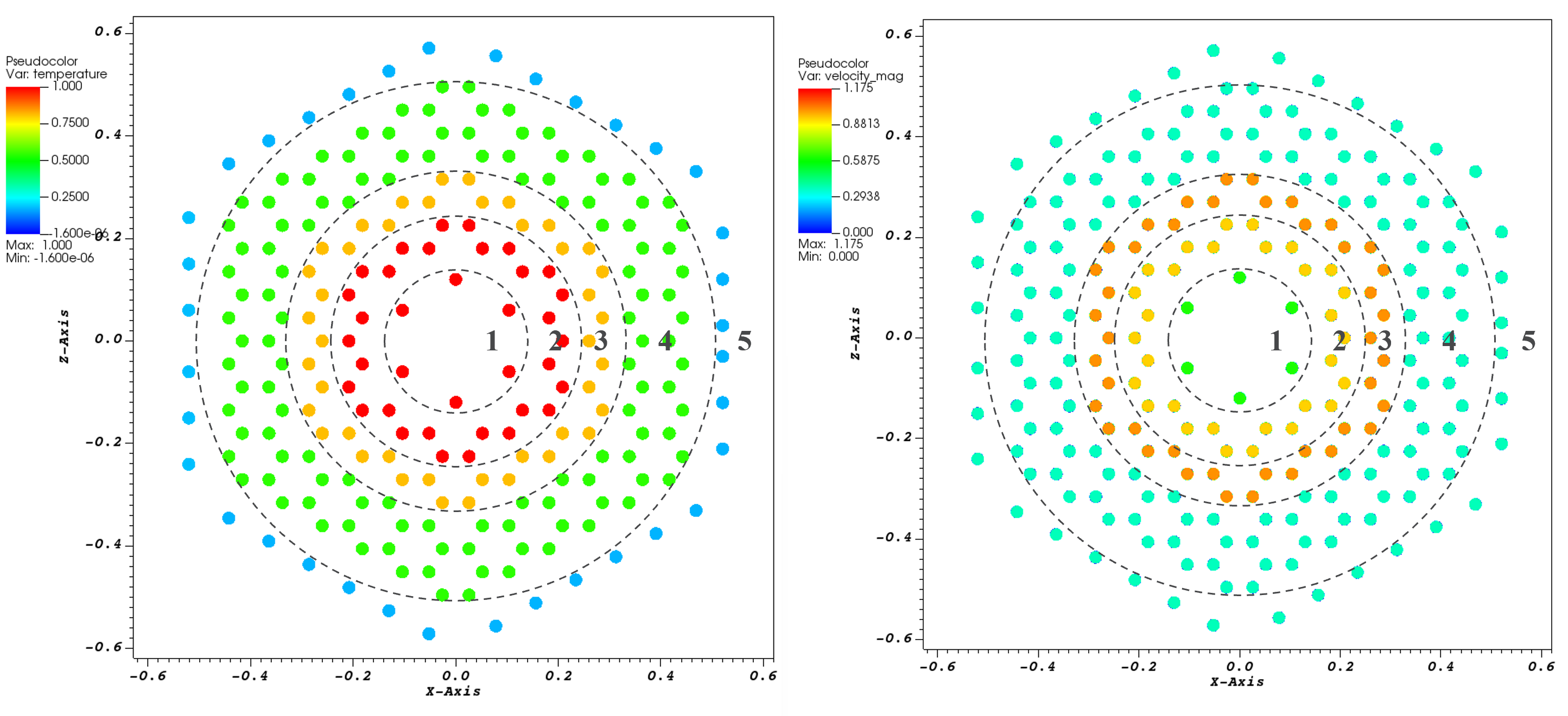
Figure 3: Inlet boundary conditions of the five inlet rings/groups: temperature (left) and velocity (right).

Table 1: Boundary conditions specified for the HTTF lower plenum CFD simulations.

Boundary	BC Type	Value
Melting temperature	$var element = document.getElementById("moose-equation-60cdb7f4-3961-4fd8-b436-4e68301c3ecf");katex.render("T_{melt}", element, {displayMode:false,throwOnError:false});$	$var element = document.getElementById("moose-equation-cb8c39bc-0723-40c1-b9df-e26926351719");katex.render("K", element, {displayMode:false,throwOnError:false});$
Ring 1	$var element = document.getElementById("moose-equation-c8e9c461-f681-4fa6-9ae9-d2c20d8fce8a");katex.render("\\dot{m}", element, {displayMode:false,throwOnError:false});$ , $var element = document.getElementById("moose-equation-7bb5d3ee-9b4f-4f55-937f-b226e7156802");katex.render("T", element, {displayMode:false,throwOnError:false});$	0.651 $var element = document.getElementById("moose-equation-87edae59-d6da-45e8-aaac-3f1ef4f504e8");katex.render("g/s", element, {displayMode:false,throwOnError:false});$ , 562.2 $var element = document.getElementById("moose-equation-1efd3f5c-9a0b-4d3a-82bf-33a6da12069e");katex.render("K", element, {displayMode:false,throwOnError:false});$
Ring 2	$var element = document.getElementById("moose-equation-02e1aac4-4e5f-478d-b9ab-58983f29577e");katex.render("\\dot{m}", element, {displayMode:false,throwOnError:false});$ , $var element = document.getElementById("moose-equation-44b3d539-9991-4124-93c1-6577555e6830");katex.render("T", element, {displayMode:false,throwOnError:false});$	4.919 $var element = document.getElementById("moose-equation-78a74e40-dd6c-4857-abb2-90bbf98416a7");katex.render("g/s", element, {displayMode:false,throwOnError:false});$ , 561.8 $var element = document.getElementById("moose-equation-4007c4e5-7d75-4031-89d0-c7be09162076");katex.render("K", element, {displayMode:false,throwOnError:false});$
Ring 3	$var element = document.getElementById("moose-equation-d465a0bb-d732-4820-8ae5-4d4885532eaa");katex.render("\\dot{m}", element, {displayMode:false,throwOnError:false});$ , $var element = document.getElementById("moose-equation-b215694e-b4d8-47c4-8fda-32973dc31eb1");katex.render("T", element, {displayMode:false,throwOnError:false});$	7.423 $var element = document.getElementById("moose-equation-b3bdd97e-6cbd-483d-9bdb-e18d810599b6");katex.render("g/s", element, {displayMode:false,throwOnError:false});$ , 541.3 $var element = document.getElementById("moose-equation-745c7c57-9bc3-47fb-95ee-47c82b0b8b15");katex.render("K", element, {displayMode:false,throwOnError:false});$
Ring 4	$var element = document.getElementById("moose-equation-86ff8fee-d5c5-4b0d-bba0-8501e2a2f43b");katex.render("\\dot{m}", element, {displayMode:false,throwOnError:false});$ , $var element = document.getElementById("moose-equation-dd066eba-1928-4b31-a63e-756fd54024d3");katex.render("T", element, {displayMode:false,throwOnError:false});$	7.704 $var element = document.getElementById("moose-equation-3f7124c3-46db-4374-8230-ede1926c040f");katex.render("g/s", element, {displayMode:false,throwOnError:false});$ , 512.0 $var element = document.getElementById("moose-equation-c36ebb38-b998-4a94-95e0-032ae905c725");katex.render("K", element, {displayMode:false,throwOnError:false});$
Ring 5	$var element = document.getElementById("moose-equation-b524193c-6da9-462e-88d2-23b672049142");katex.render("\\dot{m}", element, {displayMode:false,throwOnError:false});$ , $var element = document.getElementById("moose-equation-4518ece9-2473-4d53-854d-75fd6b996262");katex.render("T", element, {displayMode:false,throwOnError:false});$	2.337 $var element = document.getElementById("moose-equation-5c3860f6-7524-4054-a1d7-216baa4bcd6e");katex.render("g/s", element, {displayMode:false,throwOnError:false});$ , 471.6 $var element = document.getElementById("moose-equation-b78cf529-d890-4f19-813e-05031f7a26e7");katex.render("K", element, {displayMode:false,throwOnError:false});$
LP Roof	$var element = document.getElementById("moose-equation-8025377d-bd5e-4b08-ba3c-1f37409a1093");katex.render("T", element, {displayMode:false,throwOnError:false});$	543.48 $var element = document.getElementById("moose-equation-7f34f7b6-60a5-4785-a160-b69d5d09d90f");katex.render("K", element, {displayMode:false,throwOnError:false});$
LP Floor	$var element = document.getElementById("moose-equation-3e608951-cd08-4cc9-b3c4-f5a3a8db3185");katex.render("T", element, {displayMode:false,throwOnError:false});$	494.65 $var element = document.getElementById("moose-equation-73aacb51-43a1-459d-a04b-1bc431240f68");katex.render("K", element, {displayMode:false,throwOnError:false});$
Side Reflectors	$var element = document.getElementById("moose-equation-469bf289-7830-4c27-bd39-11095503f3d7");katex.render("T", element, {displayMode:false,throwOnError:false});$	452.37 $var element = document.getElementById("moose-equation-89cdf2a7-e837-438d-840e-795c648ac316");katex.render("K", element, {displayMode:false,throwOnError:false});$
LP Posts	$var element = document.getElementById("moose-equation-5811a77f-9311-43fe-9f7d-dafdd4a4174b");katex.render("T", element, {displayMode:false,throwOnError:false});$	526.39 $var element = document.getElementById("moose-equation-a98f6e8d-551d-48ff-acc0-a90694ed6bce");katex.render("K", element, {displayMode:false,throwOnError:false});$
Hot duct	$var element = document.getElementById("moose-equation-e80c2886-f396-4713-b181-8d92de59d9c2");katex.render("T", element, {displayMode:false,throwOnError:false});$	496.64 $var element = document.getElementById("moose-equation-ebb9e071-4b42-49cd-b137-1e4e62e61f6c");katex.render("K", element, {displayMode:false,throwOnError:false});$
Rakes and all other walls	Adiabatic	N/A

The mean LP pressure is 100.5 $var element = document.getElementById("moose-equation-49ffec57-c55c-4b69-b7a0-354aa4b06238");katex.render("kPa", element, {displayMode:false,throwOnError:false});$ , with which the helium gas has a density of 0.1004 $var element = document.getElementById("moose-equation-606651f6-df59-41c5-bbe9-94d70389bc3c");katex.render("kg/m^3", element, {displayMode:false,throwOnError:false});$ . A non-dimensionalization process is performed for the Nek5000 calculations. The reference velocity is 3.47 $var element = document.getElementById("moose-equation-e16efdfb-42e9-4ed5-b6b3-0fe7076ee3df");katex.render("m/s", element, {displayMode:false,throwOnError:false});$ that is the highest inlet velocity observed for Ring 3 inlet channels. The temperature difference with respect to the side reflector wall temperature (452.37 $var element = document.getElementById("moose-equation-748f7a9d-18ea-41a9-a234-185516f7ce97");katex.render("K", element, {displayMode:false,throwOnError:false});$ ) is normalized by $var element = document.getElementById("moose-equation-392c621e-ccbd-4f8a-8a06-5def92519811");katex.render("\\Delta T = 562.20-452.37 = 109.83 (K)", element, {displayMode:false,throwOnError:false});$ , where the maximum temperature is from Ring 1 inlet channels. During the post-processing, the CFD results can be easily converted back to dimensional quantities for further analyses.

Nek5000 case setups

The reader can find the Nek5000 case files and the associated HTTF lower plenum mesh files (through github LFS) in VTB repository. The mesh information is contained in two files: httf.re2 (grid coordinates, sideset ids, etc.) and httf.co2 (mesh cell connectivity). As for the Nek5000 case files, there are SIZE, httf.par, httf.usr, and two auxiliary files limits.f and utilities.f that hosts various post-processing functions, such as solution monitoring, planar averaging, and so forth. SIZE is the metafile to specify primary discretization parameters. httf.usr is the script where users specify the boundary conditions, turbulence modeling approach and post-processing. httf.par is to provide the simulation input parameters, such as material properties, time step size, Reynolds number.

Now let's dive into the most important case file httf.usr. The sideset ids contained in the mesh file are first translated into CFD boundary condition settings in usrdat2 block

      subroutine usrdat2()  ! This routine to modify mesh coordinates
      implicit none
      include 'SIZE'
      include 'TOTAL'

      real wd
      common /walldist/ wd(lx1,ly1,lz1,lelv)

      integer iel, ifc, id_face
      integer i, e, f, n
      real Dhi

      do iel=1,nelv
      do ifc=1,2*ndim
        id_face = bc(5,ifc,iel,1)
        if (id_face.eq.3) then        ! surface 1-5 for inlet
           cbc(ifc,iel,1) = 'v  '
        elseif (id_face.eq.4) then
           cbc(ifc,iel,1) = 'v  '
        elseif (id_face.eq.5) then
           cbc(ifc,iel,1) = 'v  '
        elseif (id_face.eq.6) then
           cbc(ifc,iel,1) = 'v  '
        elseif (id_face.eq.7) then
           cbc(ifc,iel,1) = 'v  '
        elseif (id_face.eq.8) then    ! surface 6-11 for walls
           cbc(ifc,iel,1) = 'W  '
        elseif (id_face.eq.9) then
           cbc(ifc,iel,1) = 'W  '
        elseif (id_face.eq.10) then
           cbc(ifc,iel,1) = 'W  '
        elseif (id_face.eq.11) then
           cbc(ifc,iel,1) = 'W  '
        elseif (id_face.eq.12) then
           cbc(ifc,iel,1) = 'W  '
        elseif (id_face.eq.13) then
           cbc(ifc,iel,1) = 'W  '
        elseif (id_face.eq.14) then    ! surface 12 for outlet
           cbc(ifc,iel,1) = 'O  '
        endif
      enddo
      enddo

      do i=2,ldimt1
      do e=1,nelt
      do f=1,ldim*2
        cbc(f,e,i)=cbc(f,e,1)
        id_face = bc(5,f,e,1)
        if(cbc(f,e,1).eq.'W  ') cbc(f,e,i)='t  '
        if(cbc(f,e,1).eq.'v  ') cbc(f,e,i)='t  '
        if(i.eq.2 .and. id_face.eq.12) cbc(f,e,i)='I  ' !Temp BC of adiabatic walls
      enddo
      enddo
      enddo

      return
      end
c-----------------------------------------------------------------------

The $var element = document.getElementById("moose-equation-dcf8fa04-62a7-462c-aab4-a5a5407ff26f");katex.render("k-\\tau", element, {displayMode:false,throwOnError:false});$ URANS model is specified in the following code block

      subroutine usrdat3()
      implicit none
      include 'SIZE'
      include 'TOTAL'

      real wd
      common /walldist/ wd(lx1,ly1,lz1,lelv)

      integer ifld_k,ifld_omg,m_id,w_id
      real coeffs(21) !array for passing your own coeffs
      logical ifcoeffs

      ifld_k = 3 !address of tke equation in t array
      ifld_omg = 4 !address of omega equation in t array
      ifcoeffs=.false. !set to true to pass your own coeffs

C     Supported models:
c     m_id = 0 !regularized high-Re k-omega (no wall functions)
c     m_id = 1 !regularized low-Re k-omega
c     m_id = 2 !regularized high-Re k-omega SST (no wall functions)
c     m_id = 3 !regularized low-Re k-omega SST
      m_id = 4 !standard k-tau model
c     m_id = 5 !low-Re   k-tau

C     Wall distance function:
c     w_id = 0 ! user specified
c     w_id = 1 ! cheap_dist (path to wall, may work better for periodic boundaries)
      w_id = 2 ! distf (coordinate difference, provides smoother function)

      call rans_init(ifld_k,ifld_omg,
     &               ifcoeffs,coeffs,w_id,wd,m_id)

      call count_boundaries

      return
      end
C-----------------------------------------------------------------------

The specific inlet temperature and mass flow rates are implemented in userbc with the non-dimensionalized values

      if(id_face.eq.3) then !Ring 1
        uy = -0.613902735
        if(ifield.eq.2) temp = 1.0
      elseif(id_face.eq.4) then !Ring 2
        uy = -0.927738111
        if(ifield.eq.2) temp = 0.996358008
      elseif(id_face.eq.5) then !Ring 3
        uy = -1.0
        if(ifield.eq.2) temp = 0.809705909
      elseif(id_face.eq.6) then !Ring 4
        uy = -0.36324936
        if(ifield.eq.2) temp = 0.542929983
      elseif(id_face.eq.7) then !Ring 5
        uy = -0.367304324
        if(ifield.eq.2) temp = 0.175088774

      elseif(id_face.eq.8) then !LP Roof
        if(ifield.eq.2) temp = 0.829554766
      elseif(id_face.eq.9) then !LP Floor
        if(ifield.eq.2) temp = 0.384958572
      elseif(id_face.eq.11) then !LP Posts
        if(ifield.eq.2) temp = 0.673950651
      elseif(id_face.eq.13) then !Hot Duct
        if(ifield.eq.2) temp = 0.403077483
      endif

Nek5000 simulation results

The aforementioned CFD cases were carried out on the Sawtooth supercomputer located at Idaho National Laboratory. A typical simulation job would use 64 compute nodes with 48 parallel processes per node. A characteristics based time-stepping has been used in the simulations to avoid the limitations imposed by the Courant-Friedrichs-Lewy (CFL) number due to the explicit treatment of the non-linear convection term. This treatment is necessary due to the existence of small local mesh cells created during the unstructured meshing and tet-to-hex conversion. A maximum CFL number of 1.75 has been reached which corresponds to an average time step size of $var element = document.getElementById("moose-equation-8c3fb669-8125-4516-a80c-f00da4e85e83");katex.render("2.5\\times 10^{-5}", element, {displayMode:false,throwOnError:false});$ . A total non-dimensional simulation time of 5.6 is achieved. Due to the nature of the unsteady RANS turbulence model, only a quasi-steady state can be reached. Velocity fluctuations are observed when helium flow enters the lower plenum and passes through the LP posts.

Snapshots of velocity and temperature fields from quasi-steady state are shown in Figure 4 and Figure 5 at the lower plenum plane ( $var element = document.getElementById("moose-equation-b41b6954-e9a4-491e-8daa-7235ca61b8ea");katex.render("y=-0.1 m", element, {displayMode:false,throwOnError:false});$ ). Significant fluctuations are observed for both velocity and temperature.

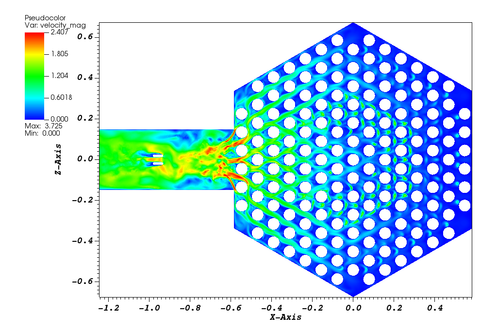
Figure 4: The quasi-steady-state velocity field (non-dimensional) in the lower plenum.

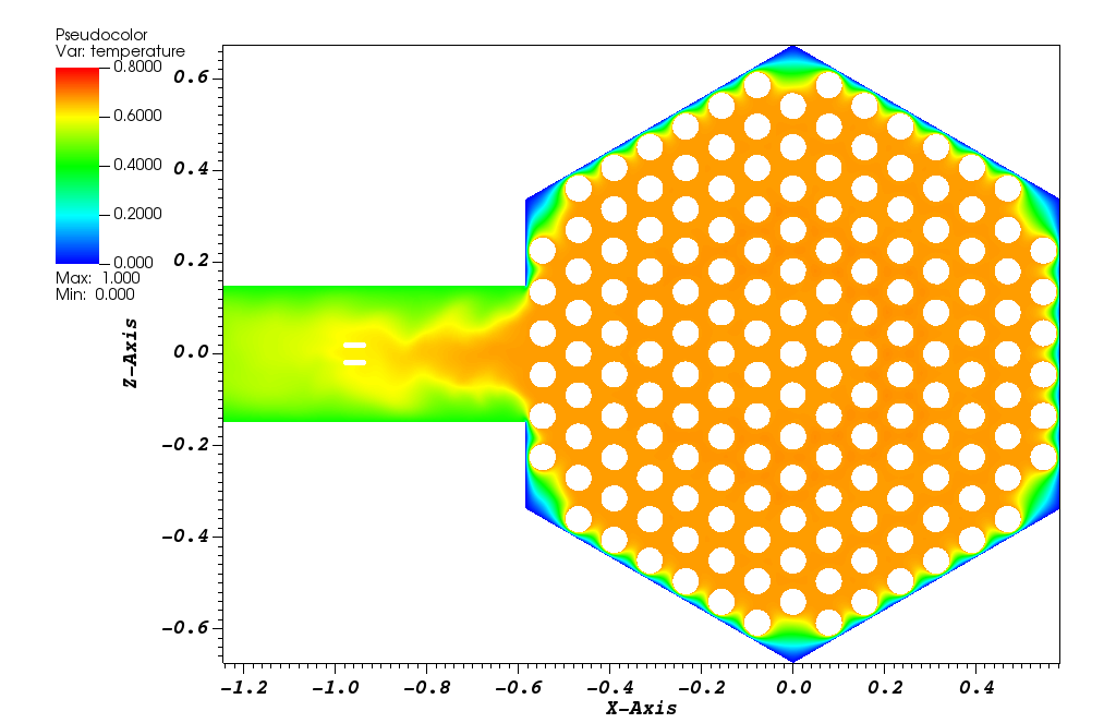
Figure 5: The quasi-steady-state temperature field (non-dimensional) in the lower plenum.

In addition to the instantaneous solutions, a time averaging analysis is also conducted for simulation results from 3.8 to 5.6 time units. Figure 6 and Figure 7 illustrate the smooth profiles of time averaged velocity and temperature field respectively. Large velocity difference is noticed due to the geometric constraints in lower plenum. On the contrary, the temperature has a more uniform distribution for the most part of lower plenum. To better understand the modeling uncertainties of numerical simulations in the related applications, the Nek5000 calculations will be compared with other CFD software's predictions. This comparative analysis will provide insights into the accuracy and reliability of the simulation results and help identify potential sources of error in the modeling process. By examining the differences and similarities between the results obtained from different software, researchers and engineers can improve the modeling techniques and optimize the simulation settings to achieve better agreement with experimental data. Such a comprehensive analysis will help to enhance the credibility and usefulness of numerical simulations for various engineering applications.

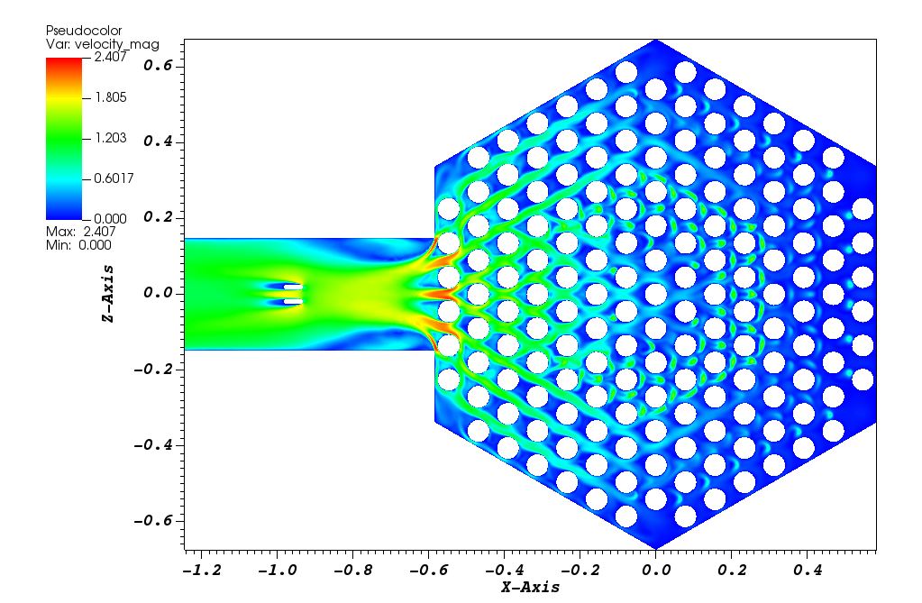
Figure 6: Time-averaged velocity field (non-dimensional) in the lower plenum.

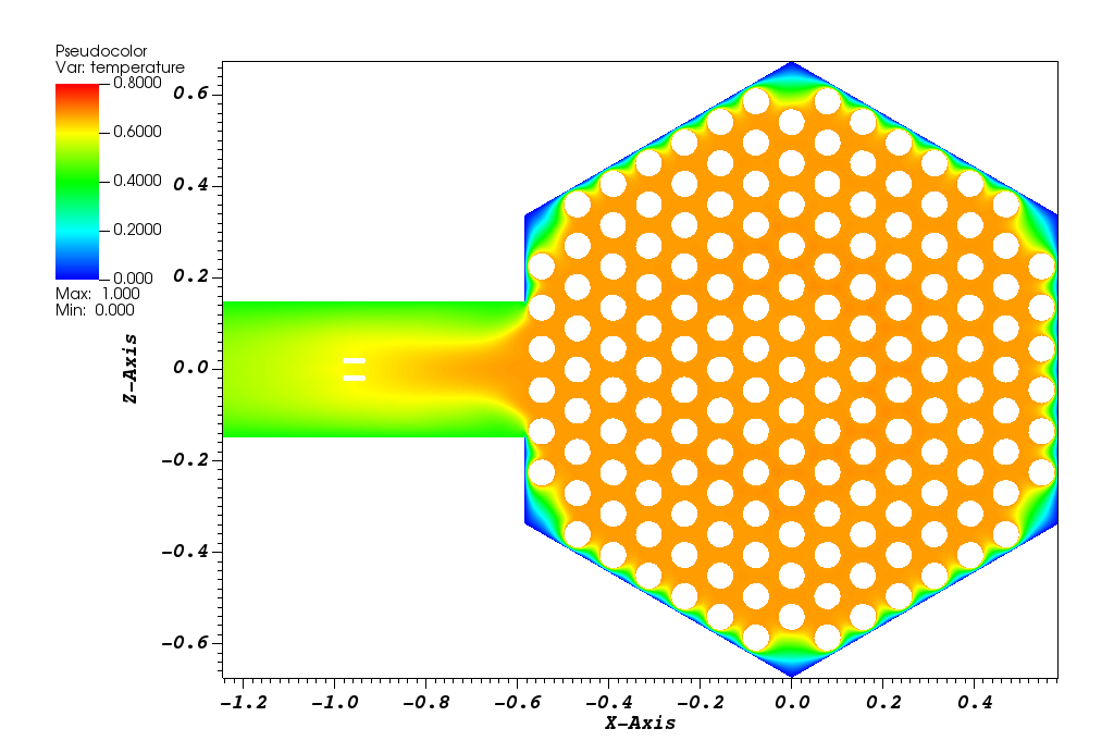
Figure 7: Time-averaged temperature field (non-dimensional) in the lower plenum.

Nek5000 run Script

To submit a Nek5000 simulation job on Sawtooth, the following batch script is used. The user can adjust the number of nodes, and number of processes per node, as well as the simulation time for any specific cases.


#!/bin/bash
#PBS -N httf
#PBS -l select=64:ncpus=48:mpiprocs=48
#PBS -l walltime=01:00:00
#PBS -j oe
#PBS -P neams
#PBS -o httf.out
cd $PBS_O_WORKDIR
export OMP_NUM_THREADS=1
echo  httf > SESSION.NAME
echo `pwd`'/' >> SESSION.NAME
rm -rf *.sch
rm -rf ioinfo
module purge
module load intel-mpi/2018.5.288-intel-19.0.5-alnu
mpirun ./nek5000 > logfile

NekRS Investigation

We initiated our simulation efforts using the Nek5000 solver. However, we opted to transition to NekRS due to its remarkable enhancement in computational efficiency. In the era of Exascale computing, there's a notable shift towards accelerated computing using Graphics Processing Units (GPUs) among leadership class supercomputers. To fully harness this new heterogeneous computing hardware, NekRS emerges as an exascale-ready thermal-fluids solver for incompressible and low-Mach number flows. Like its predecessor, Nek5000, it is based on the spectral element method and is scalable to $var element = document.getElementById("moose-equation-70927d6b-553f-4a7c-b6f4-95fd6c09b38d");katex.render("10^5", element, {displayMode:false,throwOnError:false});$ processors and beyond. The principal differences between Nek5000 and NekRS are that the former is based on F77/C, coupled with MPI and fast matrix-matrix product routines for performance, while the latter is based on C++ coupled with MPI and OCCA kernels for GPU support. The Open Concurrent Compute Abstraction provides backends for CUDA, HIP, OpenCL, and DPC++, for performance portability across all the major GPU vendors. We note that, at 80% parallel efficiency, which corresponds to 2–3 million points per MPI rank, NekRS is running at 0.1 to 0.3 seconds of wall clock time per timestep, which is nearly a 3x improvement over production runs of Nek5000 at a similar 80% strong-scale limit on CPU-based platforms.

Boundary conditions

The boundary conditions of the nekRS study are taken from the corresponding system modeling of HTTF primary loop using RELAP5-3D conducted by Canadian Nuclear Laboratories (Podila et al., 2022). The reference lower plenum pressure is 211.9 kPa, and the helium gas has a density of 0.1950 kg/m $var element = document.getElementById("moose-equation-ad32e43d-3680-4c82-8e8f-5f411c2e24e1");katex.render("^3", element, {displayMode:false,throwOnError:false});$ with a reference temperature of 895.7 K. Table 2 summarizes the key thermophysical properties of helium flow used in the NekRS simulations. The 234 inlet channels are divided into 32 groups here as shown in Figure 8 based on the radial locations and polar angles, and each group with specific mass flow rate and temperature. Inlet channels within a certain group are assumed to have the same inflow velocity corresponding to the specific mass flow rate. Details of the inlet boundary conditions are listed in Table 3. Figure 9 visually illustrates the boundary conditions that are enumerated in Table 3.

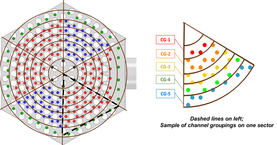
Figure 8: The grouping of lower plenum inlet channels.

Table 2: Helium thermo-physical properties and flow conditions.

$var element = document.getElementById("moose-equation-917792e6-45a5-4855-be93-1aa5adbaeb0f");katex.render("-", element, {displayMode:false,throwOnError:false});$	Value	Unit
Reference pressure	211.9	$var element = document.getElementById("moose-equation-0b468d08-9b01-47aa-b8bb-46dd178c5819");katex.render("kPa", element, {displayMode:false,throwOnError:false});$
Reference temperature	895.7	$var element = document.getElementById("moose-equation-6061e341-e9ff-41c3-9531-54de3ecf2dac");katex.render("K", element, {displayMode:false,throwOnError:false});$
Helium density	0.1075	$var element = document.getElementById("moose-equation-9a41bc6c-3a0f-47b8-b16c-badecbb95441");katex.render("kg/m^3", element, {displayMode:false,throwOnError:false});$
Helium heat capacity	5.193×10 $var element = document.getElementById("moose-equation-67aff3ea-42fb-424e-a490-d64dddc84719");katex.render("^3", element, {displayMode:false,throwOnError:false});$	$var element = document.getElementById("moose-equation-9248c640-eef0-49ba-b088-ed7867426cf6");katex.render("J/kg-K", element, {displayMode:false,throwOnError:false});$
Helium viscosity	4.274×10 $var element = document.getElementById("moose-equation-541f92b5-a1d8-4318-8184-0ac487ae1422");katex.render("^{-5}", element, {displayMode:false,throwOnError:false});$	$var element = document.getElementById("moose-equation-4c4e1dac-f747-4a2d-aedc-3ad6dfb696d0");katex.render("Pa-s", element, {displayMode:false,throwOnError:false});$
Helium thermal conductivity	0.3323	$var element = document.getElementById("moose-equation-af5f16d4-d216-48d2-b316-34905c5485e5");katex.render("W/m-K", element, {displayMode:false,throwOnError:false});$
Helium Prandtl number	0.67	$var element = document.getElementById("moose-equation-1c75d6c2-3a03-47dc-9ae3-5664d170e445");katex.render("-", element, {displayMode:false,throwOnError:false});$
Hot duct diameter	0.2984	$var element = document.getElementById("moose-equation-223a3265-e7a5-4354-8123-47b5961d3e59");katex.render("m", element, {displayMode:false,throwOnError:false});$
Mean flow velocity at Reynolds number at hot duct	41.48	$var element = document.getElementById("moose-equation-681f4cf4-c146-44a7-a642-43367d27c83d");katex.render("m/s", element, {displayMode:false,throwOnError:false});$
Reynolds number at hot duct	3.1137×10 $var element = document.getElementById("moose-equation-853234a6-d9f2-4b87-b6ec-c28d8c6ae52b");katex.render("^4", element, {displayMode:false,throwOnError:false});$	$var element = document.getElementById("moose-equation-193d061b-c60c-40b0-8756-492bd0436c01");katex.render("-", element, {displayMode:false,throwOnError:false});$

All wall surfaces are assumed to have no-slip velocity boundary condition and adiabatic thermal boundary condition. And a natural pressure condition is given to the outlet face of hot duct. The CFD simulations were carried out in a dimensionless manner. The reference velocity is the mean flow velocity at hot duct, which is 41.48 m/s. Normalization of temperature is accomplished by referencing it to the maximum inlet temperature of 984.34 K at CG0 group and the minimum inlet temperature of 810.05 K at the outer bypass group. Subsequently, during the post-processing stage, it is straightforward to convert the computational fluid dynamics (CFD) outcomes back into dimensional values, enabling additional analyses to be conducted.

Table 3: Inlet boundary conditions for the HTTF lower plenum simulations.

Zone ID	Velocity ( $var element = document.getElementById("moose-equation-ffe73a73-58a8-4562-ad80-2232790f0b95");katex.render("m/s", element, {displayMode:false,throwOnError:false});$ )	Temperature ( $var element = document.getElementById("moose-equation-faa57012-f2f6-4b37-bcff-31cff30133ea");katex.render("K", element, {displayMode:false,throwOnError:false});$ )
CG0	30.389	984.34
CG-1A	23.513	924.658
CG-2A	25.709	889.08
CG-3A	26.618	944.901
CG-4A	26.405	926.654
CG-5A	21.83	866.424
CG-1B	23.513	925.415
CG-2B	25.69	890.425
CG-3B	26.61	947.609
CG-4B	26.446	932.229
CG-5B	21.828	867.567
CG-1C	23.511	924.788
CG-2C	25.702	889.276
CG-3C	26.608	945.155
CG-4C	26.394	926.902
CG-5C	21.825	866.606
CG-1D	23.52	922.995
CG-2D	25.794	886.395
CG-3D	26.772	941.098
CG-4D	26.586	922.794
CG-5D	21.91	863.558
CG-1E	23.517	920.054
CG-2E	25.9	881.331
CG-3E	27.101	932.826
CG-4E	27.129	913.384
CG-5E	22.303	856.71
CG-1F	23.521	922.956
CG-2F	25.796	886.341
CG-3F	26.775	941.027
CG-4F	26.589	922.725
CG-5F	21.911	863.508
Outer bypass	20.669	810.051

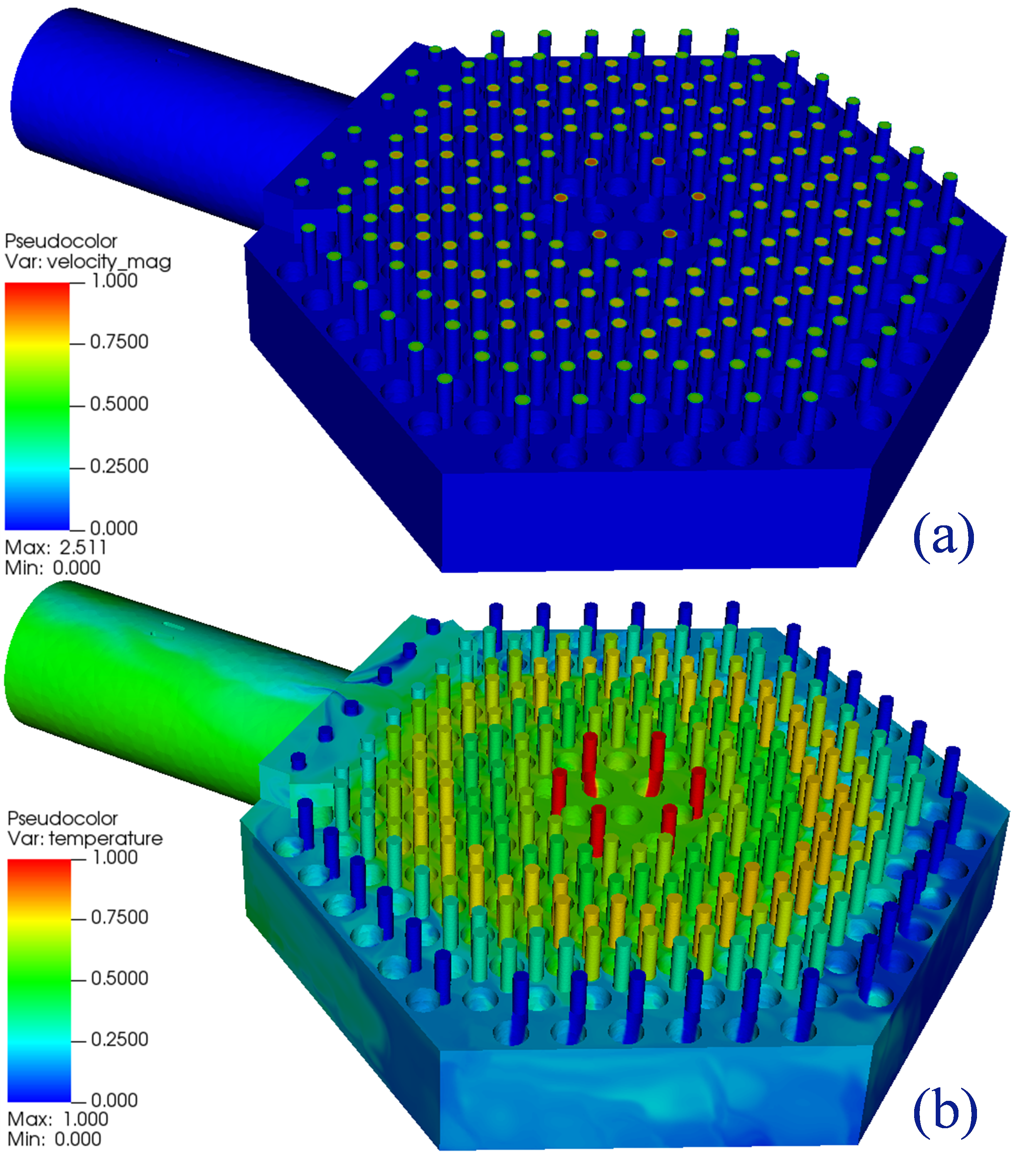
Figure 9: Boundary conditions: (a) prescribed inlet velocity and no-slip wall condition; (b) prescribed inlet temperature and adiabatic walls.

NekRS case setups

Readers can access the nekRS case files and the corresponding mesh files in the VTB repository via GitHub Large File Storage (LFS). The mesh data is contained in two files: httf.re2 (which includes grid coordinates and sideset ids) and httf.co2 (containing mesh cell connectivity information). Regarding the nekRS case files, there are four basic files:

httf.udf serves as the primary nekRS kernel file and encompasses algorithms executed on the hosts. It's responsible for configuring RANS model settings, collecting time-averaged statistics, and determining the frequency of calls to userchk, which is defined in the usr file.
httf.oudf is a supplementary file housing kernel functions for devices and also plays a role in specifying boundary conditions.
httf.usr is a legacy file inherited from Nek5000 and can be utilized to establish initial conditions and define post-processing capabilities.
httf.par is employed to input simulation parameters, including material properties, time step size, and Reynolds number.

There are also supportive scripts in the case folder. linearize_bad_elements.f and BAD_ELEMENTS are used to fix the mesh cells that potentially have negative Jacobian values from the quadratic tet-to-hex conversion. Data file InletProf.dat contains the fully developed turbulence solutions of a circular pipe, which is used to customize the profiles of velocity, TKE and tau at HTTF inlet channels.

Now let's dive into the most important case file httf.usr. The sideset ids contained in the mesh file are first translated into CFD boundary condition settings in usrdat2 block

      subroutine usrdat2()  ! This routine to modify mesh coordinates
      include 'SIZE'
      include 'TOTAL'

      integer iel, ifc, id_face
      integer i, e, f

      do iel=1,nelv
      do ifc=1,2*ndim
        id_face = bc(5,ifc,iel,1)
        if (id_face.ge.5.and.id_face.le.11) then        !CG0-CG5 and OB
           cbc(ifc,iel,1) = 'v  '
           boundaryID(ifc,iel)  = 1
           boundaryIDt(ifc,iel) = 1
        elseif (id_face.eq.4) then 			!walls
           cbc(ifc,iel,1) = 'W  '
           boundaryID(ifc,iel)  = 2
           boundaryIDt(ifc,iel) = 2
        elseif (id_face.eq.3) then                 	!outlet
           cbc(ifc,iel,1) = 'o  '
           boundaryID(ifc,iel)  = 3
           boundaryIDt(ifc,iel) = 3
        else
           cbc(ifc,iel,1) = 'E  '
           boundaryID(ifc,iel)  = 0
           boundaryIDt(ifc,iel) = 0
        endif
      enddo
      enddo

      do i=2,ldimt1
      do e=1,nelt
      do f=1,ldim*2
        cbc(f,e,i)=cbc(f,e,1)
        if(cbc(f,e,1).eq.'W  ') then
           cbc(f,e,i)='t  '
           if(i.eq.2) cbc(f,e,i)='I  '	!Insulated temp BC on walls
        endif
        if(cbc(f,e,1).eq.'v  ') cbc(f,e,i)='t  '
        if(cbc(f,e,1).eq.'o  ') cbc(f,e,i)='o  '
      enddo
      enddo
      enddo

      return
      end
c-----------------------------------------------------------------------

The fixes to the negative Jacobian errors in mesh file is called in usrdat

      subroutine usrdat   ! This routine to modify element vertices
      include 'SIZE'      ! _before_ mesh is generated, which 
      include 'TOTAL'     ! guarantees GLL mapping of mesh.

      integer n_correction
      real minJacobian
 
      n_correction = 2
      call linearize_bad_elements(n_correction)  ! 2 (iterations for correction) should be enough, if not, set to 3

      minScaleJacobian = 1e-3
      call linearize_low_jacobian_elements(n_correction,
     & minScaleJacobian) ! linearize element that with lower jacobian than minJacobian

      return
      end
c-----------------------------------------------------------------------

As for the implementation of inlet boundary conditions, a set of data arrays is created in usr and passed over to the udf and oudf. At the usr file side, the main subroutine is getinlet. It assembles the non-dimensionalized inlet velocity, temperature, k and $var element = document.getElementById("moose-equation-0c48ae5b-d3e7-4517-b53c-c9511aac089b");katex.render("\\tau", element, {displayMode:false,throwOnError:false});$ into the following arrays

      real uin,vin,win,tin
      common /inarrs/
     $     vin(lx1,ly1,lz1,lelv),
     $     t1in(lx1,ly1,lz1,lelv),
     $     t2in(lx1,ly1,lz1,lelv),
     $     t3in(lx1,ly1,lz1,lelv)

The corresponding information is transfered to httf.udf at

  //Inlet condition
  nrs->o_usrwrk = platform->device.malloc(4*nrs->fieldOffset,sizeof(dfloat));
  double *vin  = (double *) nek::scPtr(1);
  double *t1in = (double *) nek::scPtr(2);
  double *t2in = (double *) nek::scPtr(3);
  double *t3in = (double *) nek::scPtr(4);
  nrs->o_usrwrk.copyFrom(vin, mesh->Nlocal*sizeof(dfloat),0*nrs->fieldOffset*sizeof(dfloat));
  nrs->o_usrwrk.copyFrom(t1in,mesh->Nlocal*sizeof(dfloat),1*nrs->fieldOffset*sizeof(dfloat));
  nrs->o_usrwrk.copyFrom(t2in,mesh->Nlocal*sizeof(dfloat),2*nrs->fieldOffset*sizeof(dfloat));
  nrs->o_usrwrk.copyFrom(t3in,mesh->Nlocal*sizeof(dfloat),3*nrs->fieldOffset*sizeof(dfloat));
}

And then the velocity and passive scalar (temperature, k and $var element = document.getElementById("moose-equation-62efb9bc-ed83-4866-a49a-6ee19e57f3e7");katex.render("\\tau", element, {displayMode:false,throwOnError:false});$ ) boundary conditions are applied in httf.oudf at

void velocityDirichletConditions(bcData *bc)
{
  bc->u = 0.0;
  bc->v = bc->usrwrk[bc->idM + 0*bc->fieldOffset];
  bc->w = 0.0;
}

void scalarDirichletConditions(bcData *bc)
{
  bc->s = 0;
  if(bc->id==1){
    if(bc->scalarId == 0) bc->s = bc->usrwrk[bc->idM + 1*bc->fieldOffset];
    if(bc->scalarId == 1) bc->s = bc->usrwrk[bc->idM + 2*bc->fieldOffset];
    if(bc->scalarId == 2) bc->s = bc->usrwrk[bc->idM + 3*bc->fieldOffset];
  } 
}

The following code snippet in httf.udf controls the frequency that usrchk is called during the simulations, which is once in every 1,000 steps in the current case.


  if ((tstep%1000)==0){
    nek::ocopyToNek(time, tstep);
    nek::userchk();
  }

Time averaged statitics is collected using the following lines in httf.udf


  6 #include "plugins/tavg.hpp"

 45   tavg::setup(nrs);

 73   tavg::run(time);

 85   if (nrs->isOutputStep) {
 86     tavg::outfld();
 87   }

NekRS simulation results

A total simulation time of 12 non-dimensional units is achieved. Due to the nature of unsteady RANS turbulence model, only a quasi-steady state can be reached. Velocity fluctuations are observed when helium flow enters the lower plenum and passes through the LP posts. The subsequent post-processing focuses primarily on the time-averaged solutions. For that purpose, an analysis involving time-averaging is carried out on simulation results spanning from 6.0 to 12.0 time units. Figure 10 and Figure 11 portray the more uniform profiles of the time-averaged velocity and temperature distributions, respectively. Through the elimination of instantaneous fluctuations, the time-averaged outcomes reveal notably symmetric patterns in both the velocity and temperature fields. Also, Figure 10 illustrates the symmetrical horizontal jets emerging through the openings between the lower plenum posts as the helium flow enters the hot duct. Notably, flow recirculations become evident within the wake regions behind these posts.

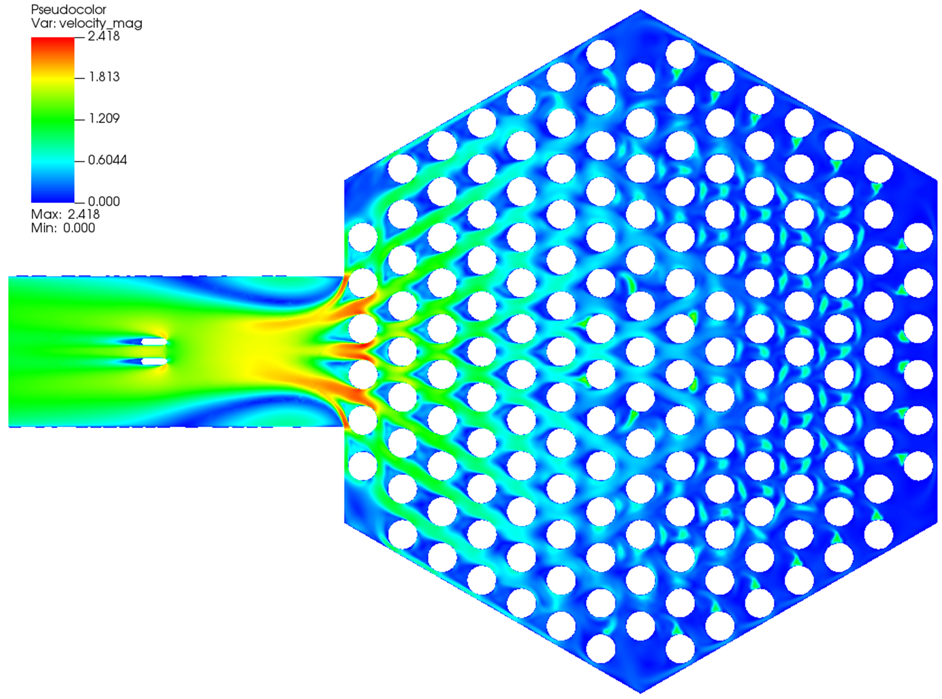
Figure 10: Time averaged velocity distribution in the lower plenum at y = -0.1 (top view).

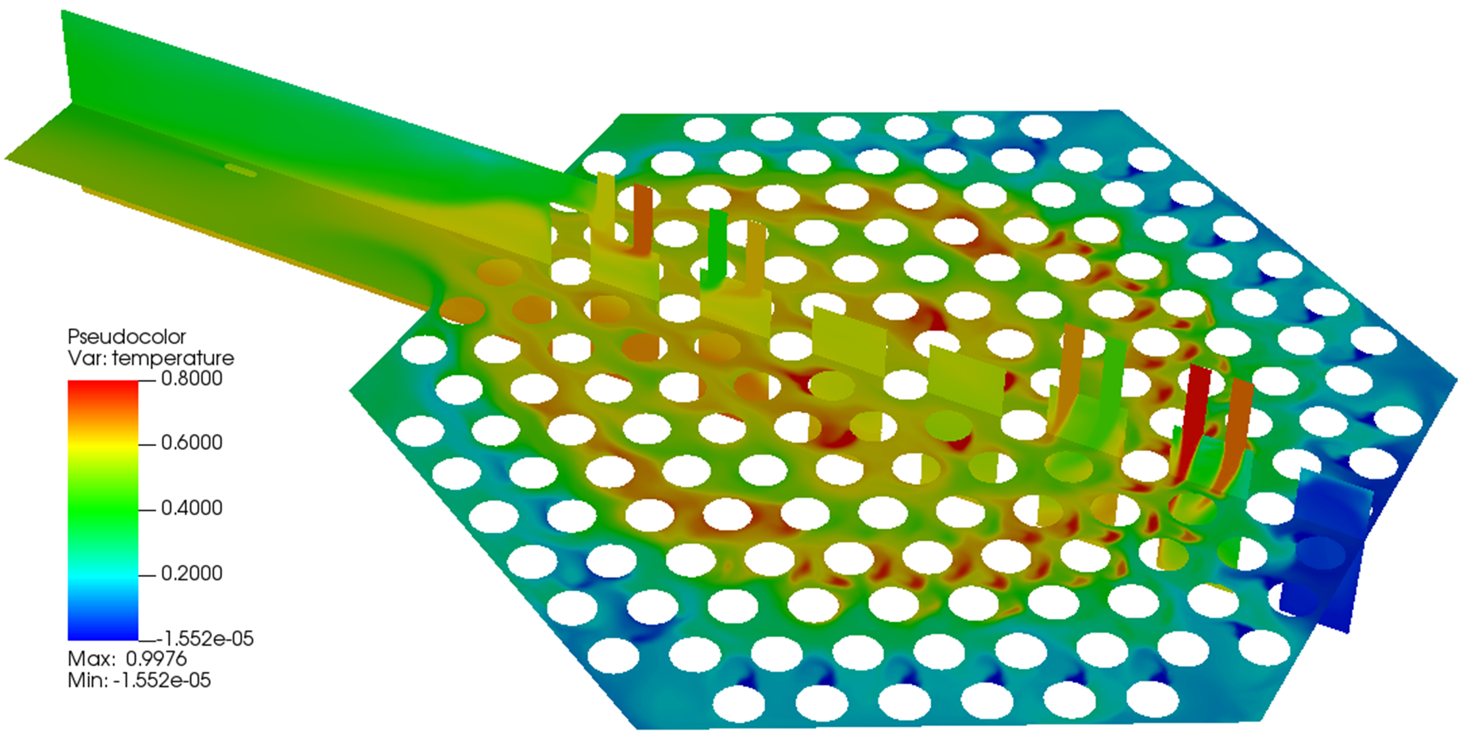
Figure 11: Time averaged temperature fields at y = -0.1 and z = 0.

In addition to the horizontal perspective, a vertical viewpoint offers a clearer insight into the injection of helium flow originating from the inlet channels. As evidenced by Figure 11 and Figure 12, the presence of helium jets is quite conspicuous within the lower plenum, characterized by notably higher velocity and temperature values. Moreover, the inflow jets exhibit greater prominence in regions farther from the hot duct, owing to the diminished local horizontal flow. Conversely, areas nearer to the hot duct showcase more pronounced disturbances in the inflow jets due to the stronger local horizontal flow. Consequently, in Figure 12, the jets positioned away from the hot duct achieve deeper penetration, while those in close proximity to the hot duct experience quicker diffusion. The presence of hot streaking is further confirmed within the lower plenum, particularly in areas distant from the hot duct. The streams of elevated temperature directly impact the lower plenum posts and floor in this specific region, resulting in uneven thermal stresses. In general, the lower section of the lower plenum encounters higher temperatures, notably at the juncture between the lower plenum and the hot duct, as visually depicted in Figure 12. Figure 13 offers an improved perspective of the temperature distribution on the lower plenum floor, enabling the identification of the hotspot.

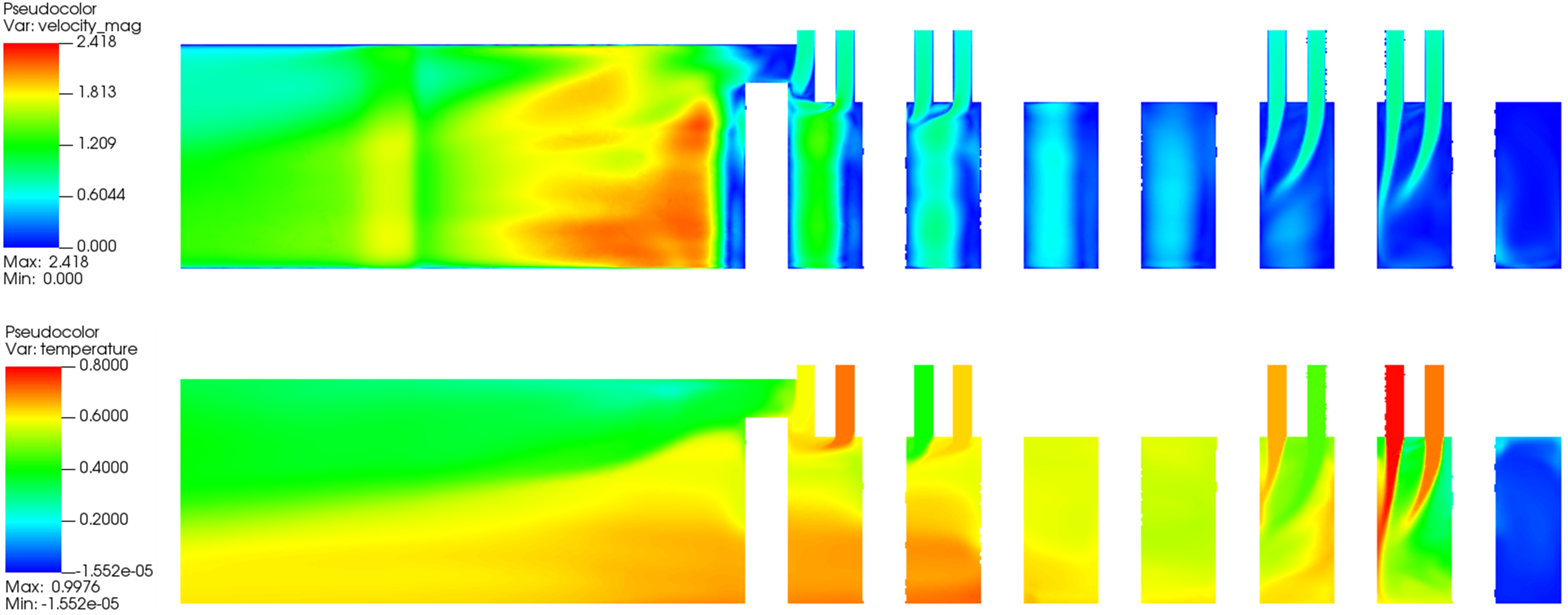
Figure 12: Jetting of helium flow from the inlet channels.

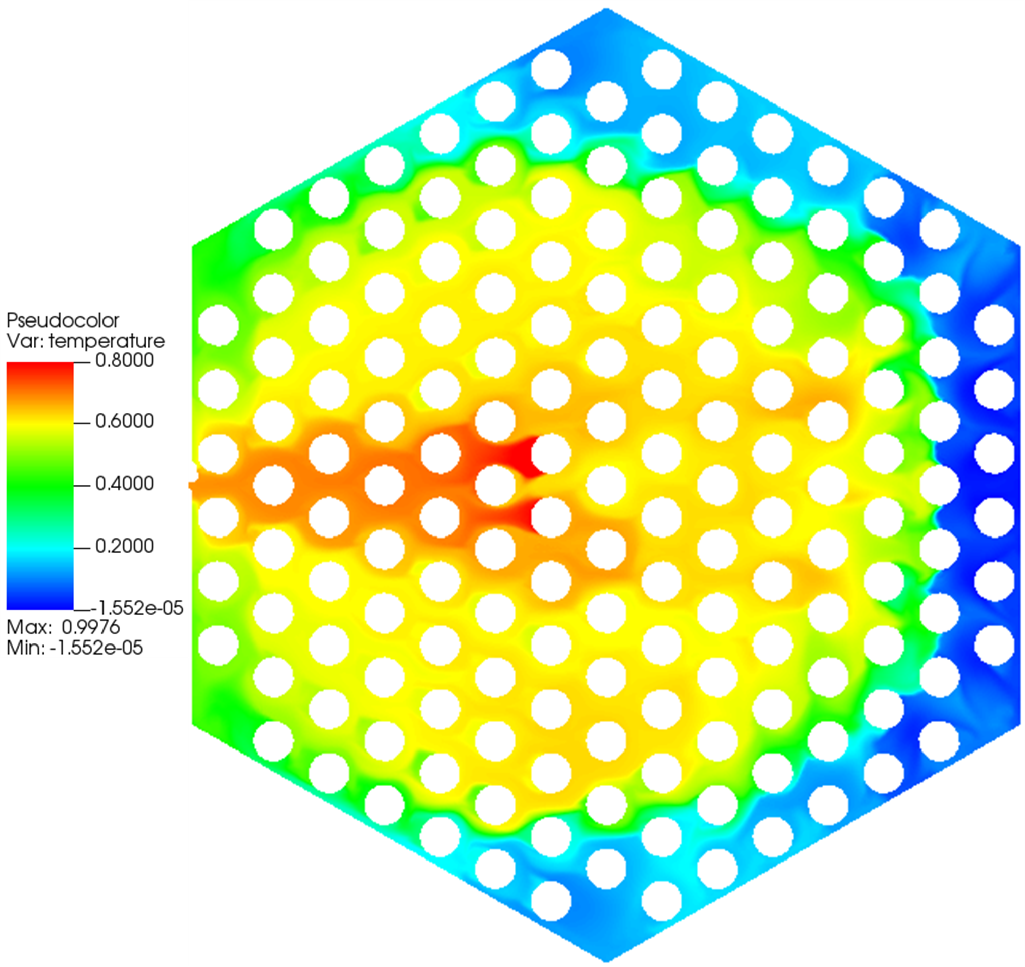
Figure 13: Time averaged temperature distribution on the lower plenum floor.

NekRS run Script

To submit a nekRS simulation job on common leadership class facilities, dedicated job submission scripts are provided in nekRS repository for supercomputers, such as Summit-OLCF, Polaris-ALCF, etc. Taking Polaris as an example, to submit the nekRS job, simply do


./nrsqsub_polaris httf 50 06:00:00

References

Sydney J Ball, M Corradini, Stephen Eugene Fisher, R Gauntt, G Geffraye, Jess C Gehin, Y Hassan, David Lewis Moses, John-Paul Renier, R Schultz, and T Wei. Next Generation Nuclear Plant Phenomena Identification and Ranking Tables (PIRTs) Volume 2: Accident and Thermal Fluids Analysis PIRTs. Technical Report NUREG/CR-6944, Oak Ridge National Laboratory, 2008. doi:10.2172/1001274.

@techreport{Ball2008,
    author = "Ball, Sydney J and Corradini, M and Fisher, Stephen Eugene and Gauntt, R and Geffraye, G and Gehin, Jess C and Hassan, Y and Moses, David Lewis and Renier, John-Paul and Schultz, R and Wei, T",
    doi = "10.2172/1001274",
    Number = "NUREG/CR-6944",
    institution = "Oak Ridge National Laboratory",
    title = "{Next Generation Nuclear Plant Phenomena Identification and Ranking Tables (PIRTs) Volume 2: Accident and Thermal Fluids Analysis PIRTs}",
    year = "2008"
}

Joshua K. Halsted. Validation analysis for the osu httf pg-28 test using relap5-3d and star-ccm+. Master's thesis, Oregon State University, 2022.

@mastersthesis{Halsted2022,
    author = "Halsted, Joshua K.",
    school = "Oregon State University",
    title = "Validation Analysis for the OSU HTTF PG-28 Test Using RELAP5-3D and STAR-CCM+",
    year = "2022"
}

K Podila, Q Chen, X Huang, C Li, Y Rao, G Waddington, and T Jafri. Coupled simulations for prismatic gas-cooled reactor. Nuclear Engineering and Design, 395:111858, 2022. URL: https://www.sciencedirect.com/science/article/pii/S0029549322002126, doi:10.1016/j.nucengdes.2022.111858.

@article{Podila2022,
    author = "Podila, K and Chen, Q and Huang, X and Li, C and Rao, Y and Waddington, G and Jafri, T",
    doi = "10.1016/j.nucengdes.2022.111858",
    issn = "0029-5493",
    journal = "Nuclear Engineering and Design",
    pages = "111858",
    title = "{Coupled simulations for prismatic gas-cooled reactor}",
    url = "https://www.sciencedirect.com/science/article/pii/S0029549322002126",
    volume = "395",
    year = "2022"
}

(htgr/httf/lower_plenum_mixing/httf.usr)

#include "experimental/rans_komg.f"
c-----------------------------------------------------------------------
c  nek5000 user-file template
c
c  user specified routines:
c     - uservp  : variable properties
c     - userf   : local acceleration term for fluid
c     - userq   : local source term for scalars
c     - userbc  : boundary conditions
c     - useric  : initial conditions
c     - userchk : general purpose routine for checking errors etc.
c     - userqtl : thermal divergence for lowMach number flows 
c     - usrdat  : modify element vertices 
c     - usrdat2 : modify mesh coordinates
c     - usrdat3 : general purpose routine for initialization
c     
c-----------------------------------------------------------------------
      include "limits.f"
      include "utilities.f"
c-----------------------------------------------------------------------
      subroutine uservp(ix,iy,iz,eg) ! set variable properties
      implicit none
      include 'SIZE'
      include 'TOTAL'
      include 'NEKUSE'

      integer ix,iy,iz,e,eg
      real rans_mut,rans_mutsk,rans_mutso
      real mu_t,Pr_t

      e = gllel(eg)

      Pr_t=0.91
      mu_t=rans_mut(ix,iy,iz,e)

      utrans = cpfld(ifield,2)
      if(ifield.eq.1) then
        udiff = cpfld(ifield,1)+mu_t
      elseif(ifield.eq.2) then
        udiff = cpfld(ifield,1)+mu_t*cpfld(ifield,2)/(Pr_t*cpfld(1,2))
      elseif(ifield.eq.3) then
        udiff = cpfld(ifield,1)+rans_mutsk(ix,iy,iz,e)
      elseif(ifield.eq.4) then
        udiff = cpfld(ifield,1)+rans_mutso(ix,iy,iz,e)
      endif

      return
      end
c-----------------------------------------------------------------------
      subroutine userf(ix,iy,iz,eg) ! set acceleration term
      implicit none
      include 'SIZE'
      include 'TOTAL'
      include 'NEKUSE'
c
c     Note: this is an acceleration term, NOT a force!
c     Thus, ffx will subsequently be multiplied by rho(x,t).
c
      integer ix,iy,iz,e,eg

      ffx = 0.0
      ffy = 0.0
      ffz = 0.0

      return
      end
c-----------------------------------------------------------------------
      subroutine userq(ix,iy,iz,eg) ! set source term
      implicit none
      include 'SIZE'
      include 'TOTAL'
      include 'NEKUSE'

      integer ix,iy,iz,e,eg
      real rans_kSrc,rans_omgSrc
      real rans_kDiag,rans_omgDiag

      e = gllel(eg)

      if(ifield.eq.3) then
        qvol = rans_kSrc(ix,iy,iz,e)
        avol = rans_kDiag(ix,iy,iz,e)
      elseif(ifield.eq.4) then
        qvol = rans_omgSrc(ix,iy,iz,e)
        avol = rans_omgDiag(ix,iy,iz,e)
      else
        qvol = 0.0
      endif

      return
      end
c-----------------------------------------------------------------------
      subroutine userbc(ix,iy,iz,iside,eg) ! set up boundary conditions
      implicit none
      include 'SIZE'
      include 'TOTAL'
      include 'NEKUSE'

      real wd
      common /walldist/ wd(lx1,ly1,lz1,lelv)

      integer ix,iy,iz,iside,e,eg,id_face
      real tke_tmp,tau_tmp

      e = gllel(eg)

      id_face = bc(5,iside,e,1)

      ux   = 0.0
      uy   = 0.0
      uz   = 0.0
      temp = 0.0

      if(id_face.eq.3) then !Ring 1
        uy = -0.613902735
        if(ifield.eq.2) temp = 1.0
      elseif(id_face.eq.4) then !Ring 2
        uy = -0.927738111
        if(ifield.eq.2) temp = 0.996358008
      elseif(id_face.eq.5) then !Ring 3
        uy = -1.0
        if(ifield.eq.2) temp = 0.809705909
      elseif(id_face.eq.6) then !Ring 4
        uy = -0.36324936
        if(ifield.eq.2) temp = 0.542929983
      elseif(id_face.eq.7) then !Ring 5
        uy = -0.367304324
        if(ifield.eq.2) temp = 0.175088774

      elseif(id_face.eq.8) then !LP Roof
        if(ifield.eq.2) temp = 0.829554766
      elseif(id_face.eq.9) then !LP Floor
        if(ifield.eq.2) temp = 0.384958572
      elseif(id_face.eq.11) then !LP Posts
        if(ifield.eq.2) temp = 0.673950651
      elseif(id_face.eq.13) then !Hot Duct
        if(ifield.eq.2) temp = 0.403077483
      endif

      call turb_in(wd(ix,iy,iz,e),tke_tmp,tau_tmp)
      if(ifield.eq.3) temp = tke_tmp
      if(ifield.eq.4) temp = tau_tmp

      return
      end
c-----------------------------------------------------------------------
      subroutine useric(ix,iy,iz,eg) ! set up initial conditions
      implicit none
      include 'SIZE'
      include 'TOTAL'
      include 'NEKUSE'

      real wd
      common /walldist/ wd(lx1,ly1,lz1,lelv)

      integer ix,iy,iz,e,eg
      real tke_tmp,tau_tmp 

      e = gllel(eg)

      ux   = 0.0
      uy   = 0.0
      uz   = 0.0
      temp = 0.0

      call turb_in(wd(ix,iy,iz,e),tke_tmp,tau_tmp)
      if(ifield.eq.3) temp = tke_tmp
      if(ifield.eq.4) temp = tau_tmp

      return
      end
c-----------------------------------------------------------------------
      subroutine userchk()
      implicit none
      include 'SIZE'
      include 'TOTAL'

      integer lt,i,ntot
      parameter(lt=lx1*ly1*lz1*lelv)

      real wd
      common /walldist/ wd(lx1,ly1,lz1,lelv)
      real norm(3),pt(3),eps,planar_ave_m1,umean,pmean

      norm(1) = 1.0
      norm(2) = 0.0
      norm(3) = 0.0
      pt(1) =-1.2
      pt(2) = 0.0
      pt(3) = 0.0
      eps = 0.02

      if(mod(istep,100).eq.0) then
        call print_limits 
        call y_p_limits(wd,.true.)
      endif
      umean=planar_ave_m1(vx,norm,pt,eps)
      pmean=planar_ave_m1(pr,norm,pt,eps)
      if(nio.eq.0) then
        write(6,'(a15,es13.4)') "umean:",umean
        write(6,'(a15,es13.4)') "pmean:",pmean
        write(6,*)
      endif

      call avg_all

      return
      end
c-----------------------------------------------------------------------
      subroutine userqtl ! Set thermal divergence

      call userqtl_scig 

      return
      end
c-----------------------------------------------------------------------
      subroutine usrdat()   ! This routine to modify element vertices
      implicit none
      include 'SIZE'
      include 'TOTAL'

      return
      end
c-----------------------------------------------------------------------
      subroutine usrdat2()  ! This routine to modify mesh coordinates
      implicit none
      include 'SIZE'
      include 'TOTAL'

      real wd
      common /walldist/ wd(lx1,ly1,lz1,lelv)

      integer iel, ifc, id_face
      integer i, e, f, n
      real Dhi

      do iel=1,nelv
      do ifc=1,2*ndim
        id_face = bc(5,ifc,iel,1)
        if (id_face.eq.3) then        ! surface 1-5 for inlet
           cbc(ifc,iel,1) = 'v  '
        elseif (id_face.eq.4) then
           cbc(ifc,iel,1) = 'v  '
        elseif (id_face.eq.5) then
           cbc(ifc,iel,1) = 'v  '
        elseif (id_face.eq.6) then
           cbc(ifc,iel,1) = 'v  '
        elseif (id_face.eq.7) then
           cbc(ifc,iel,1) = 'v  '
        elseif (id_face.eq.8) then    ! surface 6-11 for walls
           cbc(ifc,iel,1) = 'W  '
        elseif (id_face.eq.9) then
           cbc(ifc,iel,1) = 'W  '
        elseif (id_face.eq.10) then
           cbc(ifc,iel,1) = 'W  '
        elseif (id_face.eq.11) then
           cbc(ifc,iel,1) = 'W  '
        elseif (id_face.eq.12) then
           cbc(ifc,iel,1) = 'W  '
        elseif (id_face.eq.13) then
           cbc(ifc,iel,1) = 'W  '
        elseif (id_face.eq.14) then    ! surface 12 for outlet
           cbc(ifc,iel,1) = 'O  '
        endif
      enddo
      enddo

      do i=2,ldimt1
      do e=1,nelt
      do f=1,ldim*2
        cbc(f,e,i)=cbc(f,e,1)
        id_face = bc(5,f,e,1)
        if(cbc(f,e,1).eq.'W  ') cbc(f,e,i)='t  '
        if(cbc(f,e,1).eq.'v  ') cbc(f,e,i)='t  '
        if(i.eq.2 .and. id_face.eq.12) cbc(f,e,i)='I  ' !Temp BC of adiabatic walls
      enddo
      enddo
      enddo

      return
      end
c-----------------------------------------------------------------------
      subroutine usrdat3()
      implicit none
      include 'SIZE'
      include 'TOTAL'

      real wd
      common /walldist/ wd(lx1,ly1,lz1,lelv)

      integer ifld_k,ifld_omg,m_id,w_id
      real coeffs(21) !array for passing your own coeffs
      logical ifcoeffs

      ifld_k = 3 !address of tke equation in t array
      ifld_omg = 4 !address of omega equation in t array
      ifcoeffs=.false. !set to true to pass your own coeffs

C     Supported models:
c     m_id = 0 !regularized high-Re k-omega (no wall functions)
c     m_id = 1 !regularized low-Re k-omega
c     m_id = 2 !regularized high-Re k-omega SST (no wall functions)
c     m_id = 3 !regularized low-Re k-omega SST
      m_id = 4 !standard k-tau model
c     m_id = 5 !low-Re   k-tau

C     Wall distance function:
c     w_id = 0 ! user specified
c     w_id = 1 ! cheap_dist (path to wall, may work better for periodic boundaries)
      w_id = 2 ! distf (coordinate difference, provides smoother function)

      call rans_init(ifld_k,ifld_omg,
     &               ifcoeffs,coeffs,w_id,wd,m_id)

      call count_boundaries

      return
      end
C-----------------------------------------------------------------------
      subroutine turb_in(wd,tke,tau)
      include 'SIZE'
      include 'TOTAL'

      integer ix,iy,iz,e
      real wd,tke,tau

      real Re,darcy,utau,sigk,kmax,yplus,yk

      Re = 1.0/param(2)
      darcy = 0.316/(Re**0.25)
      utau = sqrt(darcy/8.0)
      sigk = 0.6
      kmax = 2.5*utau*utau
      yplus = max(wd*utau*Re,1.0e-6)
      yk=30.0

      tke=kmax*exp(-(log10(yplus/yk))**2.0/(2.0*sigk**2))
      tau=0.012*wd**2.0/cpfld(ifield,1)

      return
      end
c-----------------------------------------------------------------------

(htgr/httf/lower_plenum_mixing/httf.usr)

#include "experimental/rans_komg.f"
c-----------------------------------------------------------------------
c  nek5000 user-file template
c
c  user specified routines:
c     - uservp  : variable properties
c     - userf   : local acceleration term for fluid
c     - userq   : local source term for scalars
c     - userbc  : boundary conditions
c     - useric  : initial conditions
c     - userchk : general purpose routine for checking errors etc.
c     - userqtl : thermal divergence for lowMach number flows 
c     - usrdat  : modify element vertices 
c     - usrdat2 : modify mesh coordinates
c     - usrdat3 : general purpose routine for initialization
c     
c-----------------------------------------------------------------------
      include "limits.f"
      include "utilities.f"
c-----------------------------------------------------------------------
      subroutine uservp(ix,iy,iz,eg) ! set variable properties
      implicit none
      include 'SIZE'
      include 'TOTAL'
      include 'NEKUSE'

      integer ix,iy,iz,e,eg
      real rans_mut,rans_mutsk,rans_mutso
      real mu_t,Pr_t

      e = gllel(eg)

      Pr_t=0.91
      mu_t=rans_mut(ix,iy,iz,e)

      utrans = cpfld(ifield,2)
      if(ifield.eq.1) then
        udiff = cpfld(ifield,1)+mu_t
      elseif(ifield.eq.2) then
        udiff = cpfld(ifield,1)+mu_t*cpfld(ifield,2)/(Pr_t*cpfld(1,2))
      elseif(ifield.eq.3) then
        udiff = cpfld(ifield,1)+rans_mutsk(ix,iy,iz,e)
      elseif(ifield.eq.4) then
        udiff = cpfld(ifield,1)+rans_mutso(ix,iy,iz,e)
      endif

      return
      end
c-----------------------------------------------------------------------
      subroutine userf(ix,iy,iz,eg) ! set acceleration term
      implicit none
      include 'SIZE'
      include 'TOTAL'
      include 'NEKUSE'
c
c     Note: this is an acceleration term, NOT a force!
c     Thus, ffx will subsequently be multiplied by rho(x,t).
c
      integer ix,iy,iz,e,eg

      ffx = 0.0
      ffy = 0.0
      ffz = 0.0

      return
      end
c-----------------------------------------------------------------------
      subroutine userq(ix,iy,iz,eg) ! set source term
      implicit none
      include 'SIZE'
      include 'TOTAL'
      include 'NEKUSE'

      integer ix,iy,iz,e,eg
      real rans_kSrc,rans_omgSrc
      real rans_kDiag,rans_omgDiag

      e = gllel(eg)

      if(ifield.eq.3) then
        qvol = rans_kSrc(ix,iy,iz,e)
        avol = rans_kDiag(ix,iy,iz,e)
      elseif(ifield.eq.4) then
        qvol = rans_omgSrc(ix,iy,iz,e)
        avol = rans_omgDiag(ix,iy,iz,e)
      else
        qvol = 0.0
      endif

      return
      end
c-----------------------------------------------------------------------
      subroutine userbc(ix,iy,iz,iside,eg) ! set up boundary conditions
      implicit none
      include 'SIZE'
      include 'TOTAL'
      include 'NEKUSE'

      real wd
      common /walldist/ wd(lx1,ly1,lz1,lelv)

      integer ix,iy,iz,iside,e,eg,id_face
      real tke_tmp,tau_tmp

      e = gllel(eg)

      id_face = bc(5,iside,e,1)

      ux   = 0.0
      uy   = 0.0
      uz   = 0.0
      temp = 0.0

      if(id_face.eq.3) then !Ring 1
        uy = -0.613902735
        if(ifield.eq.2) temp = 1.0
      elseif(id_face.eq.4) then !Ring 2
        uy = -0.927738111
        if(ifield.eq.2) temp = 0.996358008
      elseif(id_face.eq.5) then !Ring 3
        uy = -1.0
        if(ifield.eq.2) temp = 0.809705909
      elseif(id_face.eq.6) then !Ring 4
        uy = -0.36324936
        if(ifield.eq.2) temp = 0.542929983
      elseif(id_face.eq.7) then !Ring 5
        uy = -0.367304324
        if(ifield.eq.2) temp = 0.175088774

      elseif(id_face.eq.8) then !LP Roof
        if(ifield.eq.2) temp = 0.829554766
      elseif(id_face.eq.9) then !LP Floor
        if(ifield.eq.2) temp = 0.384958572
      elseif(id_face.eq.11) then !LP Posts
        if(ifield.eq.2) temp = 0.673950651
      elseif(id_face.eq.13) then !Hot Duct
        if(ifield.eq.2) temp = 0.403077483
      endif

      call turb_in(wd(ix,iy,iz,e),tke_tmp,tau_tmp)
      if(ifield.eq.3) temp = tke_tmp
      if(ifield.eq.4) temp = tau_tmp

      return
      end
c-----------------------------------------------------------------------
      subroutine useric(ix,iy,iz,eg) ! set up initial conditions
      implicit none
      include 'SIZE'
      include 'TOTAL'
      include 'NEKUSE'

      real wd
      common /walldist/ wd(lx1,ly1,lz1,lelv)

      integer ix,iy,iz,e,eg
      real tke_tmp,tau_tmp 

      e = gllel(eg)

      ux   = 0.0
      uy   = 0.0
      uz   = 0.0
      temp = 0.0

      call turb_in(wd(ix,iy,iz,e),tke_tmp,tau_tmp)
      if(ifield.eq.3) temp = tke_tmp
      if(ifield.eq.4) temp = tau_tmp

      return
      end
c-----------------------------------------------------------------------
      subroutine userchk()
      implicit none
      include 'SIZE'
      include 'TOTAL'

      integer lt,i,ntot
      parameter(lt=lx1*ly1*lz1*lelv)

      real wd
      common /walldist/ wd(lx1,ly1,lz1,lelv)
      real norm(3),pt(3),eps,planar_ave_m1,umean,pmean

      norm(1) = 1.0
      norm(2) = 0.0
      norm(3) = 0.0
      pt(1) =-1.2
      pt(2) = 0.0
      pt(3) = 0.0
      eps = 0.02

      if(mod(istep,100).eq.0) then
        call print_limits 
        call y_p_limits(wd,.true.)
      endif
      umean=planar_ave_m1(vx,norm,pt,eps)
      pmean=planar_ave_m1(pr,norm,pt,eps)
      if(nio.eq.0) then
        write(6,'(a15,es13.4)') "umean:",umean
        write(6,'(a15,es13.4)') "pmean:",pmean
        write(6,*)
      endif

      call avg_all

      return
      end
c-----------------------------------------------------------------------
      subroutine userqtl ! Set thermal divergence

      call userqtl_scig 

      return
      end
c-----------------------------------------------------------------------
      subroutine usrdat()   ! This routine to modify element vertices
      implicit none
      include 'SIZE'
      include 'TOTAL'

      return
      end
c-----------------------------------------------------------------------
      subroutine usrdat2()  ! This routine to modify mesh coordinates
      implicit none
      include 'SIZE'
      include 'TOTAL'

      real wd
      common /walldist/ wd(lx1,ly1,lz1,lelv)

      integer iel, ifc, id_face
      integer i, e, f, n
      real Dhi

      do iel=1,nelv
      do ifc=1,2*ndim
        id_face = bc(5,ifc,iel,1)
        if (id_face.eq.3) then        ! surface 1-5 for inlet
           cbc(ifc,iel,1) = 'v  '
        elseif (id_face.eq.4) then
           cbc(ifc,iel,1) = 'v  '
        elseif (id_face.eq.5) then
           cbc(ifc,iel,1) = 'v  '
        elseif (id_face.eq.6) then
           cbc(ifc,iel,1) = 'v  '
        elseif (id_face.eq.7) then
           cbc(ifc,iel,1) = 'v  '
        elseif (id_face.eq.8) then    ! surface 6-11 for walls
           cbc(ifc,iel,1) = 'W  '
        elseif (id_face.eq.9) then
           cbc(ifc,iel,1) = 'W  '
        elseif (id_face.eq.10) then
           cbc(ifc,iel,1) = 'W  '
        elseif (id_face.eq.11) then
           cbc(ifc,iel,1) = 'W  '
        elseif (id_face.eq.12) then
           cbc(ifc,iel,1) = 'W  '
        elseif (id_face.eq.13) then
           cbc(ifc,iel,1) = 'W  '
        elseif (id_face.eq.14) then    ! surface 12 for outlet
           cbc(ifc,iel,1) = 'O  '
        endif
      enddo
      enddo

      do i=2,ldimt1
      do e=1,nelt
      do f=1,ldim*2
        cbc(f,e,i)=cbc(f,e,1)
        id_face = bc(5,f,e,1)
        if(cbc(f,e,1).eq.'W  ') cbc(f,e,i)='t  '
        if(cbc(f,e,1).eq.'v  ') cbc(f,e,i)='t  '
        if(i.eq.2 .and. id_face.eq.12) cbc(f,e,i)='I  ' !Temp BC of adiabatic walls
      enddo
      enddo
      enddo

      return
      end
c-----------------------------------------------------------------------
      subroutine usrdat3()
      implicit none
      include 'SIZE'
      include 'TOTAL'

      real wd
      common /walldist/ wd(lx1,ly1,lz1,lelv)

      integer ifld_k,ifld_omg,m_id,w_id
      real coeffs(21) !array for passing your own coeffs
      logical ifcoeffs

      ifld_k = 3 !address of tke equation in t array
      ifld_omg = 4 !address of omega equation in t array
      ifcoeffs=.false. !set to true to pass your own coeffs

C     Supported models:
c     m_id = 0 !regularized high-Re k-omega (no wall functions)
c     m_id = 1 !regularized low-Re k-omega
c     m_id = 2 !regularized high-Re k-omega SST (no wall functions)
c     m_id = 3 !regularized low-Re k-omega SST
      m_id = 4 !standard k-tau model
c     m_id = 5 !low-Re   k-tau

C     Wall distance function:
c     w_id = 0 ! user specified
c     w_id = 1 ! cheap_dist (path to wall, may work better for periodic boundaries)
      w_id = 2 ! distf (coordinate difference, provides smoother function)

      call rans_init(ifld_k,ifld_omg,
     &               ifcoeffs,coeffs,w_id,wd,m_id)

      call count_boundaries

      return
      end
C-----------------------------------------------------------------------
      subroutine turb_in(wd,tke,tau)
      include 'SIZE'
      include 'TOTAL'

      integer ix,iy,iz,e
      real wd,tke,tau

      real Re,darcy,utau,sigk,kmax,yplus,yk

      Re = 1.0/param(2)
      darcy = 0.316/(Re**0.25)
      utau = sqrt(darcy/8.0)
      sigk = 0.6
      kmax = 2.5*utau*utau
      yplus = max(wd*utau*Re,1.0e-6)
      yk=30.0

      tke=kmax*exp(-(log10(yplus/yk))**2.0/(2.0*sigk**2))
      tau=0.012*wd**2.0/cpfld(ifield,1)

      return
      end
c-----------------------------------------------------------------------

(htgr/httf/lower_plenum_mixing/httf.usr)

#include "experimental/rans_komg.f"
c-----------------------------------------------------------------------
c  nek5000 user-file template
c
c  user specified routines:
c     - uservp  : variable properties
c     - userf   : local acceleration term for fluid
c     - userq   : local source term for scalars
c     - userbc  : boundary conditions
c     - useric  : initial conditions
c     - userchk : general purpose routine for checking errors etc.
c     - userqtl : thermal divergence for lowMach number flows 
c     - usrdat  : modify element vertices 
c     - usrdat2 : modify mesh coordinates
c     - usrdat3 : general purpose routine for initialization
c     
c-----------------------------------------------------------------------
      include "limits.f"
      include "utilities.f"
c-----------------------------------------------------------------------
      subroutine uservp(ix,iy,iz,eg) ! set variable properties
      implicit none
      include 'SIZE'
      include 'TOTAL'
      include 'NEKUSE'

      integer ix,iy,iz,e,eg
      real rans_mut,rans_mutsk,rans_mutso
      real mu_t,Pr_t

      e = gllel(eg)

      Pr_t=0.91
      mu_t=rans_mut(ix,iy,iz,e)

      utrans = cpfld(ifield,2)
      if(ifield.eq.1) then
        udiff = cpfld(ifield,1)+mu_t
      elseif(ifield.eq.2) then
        udiff = cpfld(ifield,1)+mu_t*cpfld(ifield,2)/(Pr_t*cpfld(1,2))
      elseif(ifield.eq.3) then
        udiff = cpfld(ifield,1)+rans_mutsk(ix,iy,iz,e)
      elseif(ifield.eq.4) then
        udiff = cpfld(ifield,1)+rans_mutso(ix,iy,iz,e)
      endif

      return
      end
c-----------------------------------------------------------------------
      subroutine userf(ix,iy,iz,eg) ! set acceleration term
      implicit none
      include 'SIZE'
      include 'TOTAL'
      include 'NEKUSE'
c
c     Note: this is an acceleration term, NOT a force!
c     Thus, ffx will subsequently be multiplied by rho(x,t).
c
      integer ix,iy,iz,e,eg

      ffx = 0.0
      ffy = 0.0
      ffz = 0.0

      return
      end
c-----------------------------------------------------------------------
      subroutine userq(ix,iy,iz,eg) ! set source term
      implicit none
      include 'SIZE'
      include 'TOTAL'
      include 'NEKUSE'

      integer ix,iy,iz,e,eg
      real rans_kSrc,rans_omgSrc
      real rans_kDiag,rans_omgDiag

      e = gllel(eg)

      if(ifield.eq.3) then
        qvol = rans_kSrc(ix,iy,iz,e)
        avol = rans_kDiag(ix,iy,iz,e)
      elseif(ifield.eq.4) then
        qvol = rans_omgSrc(ix,iy,iz,e)
        avol = rans_omgDiag(ix,iy,iz,e)
      else
        qvol = 0.0
      endif

      return
      end
c-----------------------------------------------------------------------
      subroutine userbc(ix,iy,iz,iside,eg) ! set up boundary conditions
      implicit none
      include 'SIZE'
      include 'TOTAL'
      include 'NEKUSE'

      real wd
      common /walldist/ wd(lx1,ly1,lz1,lelv)

      integer ix,iy,iz,iside,e,eg,id_face
      real tke_tmp,tau_tmp

      e = gllel(eg)

      id_face = bc(5,iside,e,1)

      ux   = 0.0
      uy   = 0.0
      uz   = 0.0
      temp = 0.0

      if(id_face.eq.3) then !Ring 1
        uy = -0.613902735
        if(ifield.eq.2) temp = 1.0
      elseif(id_face.eq.4) then !Ring 2
        uy = -0.927738111
        if(ifield.eq.2) temp = 0.996358008
      elseif(id_face.eq.5) then !Ring 3
        uy = -1.0
        if(ifield.eq.2) temp = 0.809705909
      elseif(id_face.eq.6) then !Ring 4
        uy = -0.36324936
        if(ifield.eq.2) temp = 0.542929983
      elseif(id_face.eq.7) then !Ring 5
        uy = -0.367304324
        if(ifield.eq.2) temp = 0.175088774

      elseif(id_face.eq.8) then !LP Roof
        if(ifield.eq.2) temp = 0.829554766
      elseif(id_face.eq.9) then !LP Floor
        if(ifield.eq.2) temp = 0.384958572
      elseif(id_face.eq.11) then !LP Posts
        if(ifield.eq.2) temp = 0.673950651
      elseif(id_face.eq.13) then !Hot Duct
        if(ifield.eq.2) temp = 0.403077483
      endif

      call turb_in(wd(ix,iy,iz,e),tke_tmp,tau_tmp)
      if(ifield.eq.3) temp = tke_tmp
      if(ifield.eq.4) temp = tau_tmp

      return
      end
c-----------------------------------------------------------------------
      subroutine useric(ix,iy,iz,eg) ! set up initial conditions
      implicit none
      include 'SIZE'
      include 'TOTAL'
      include 'NEKUSE'

      real wd
      common /walldist/ wd(lx1,ly1,lz1,lelv)

      integer ix,iy,iz,e,eg
      real tke_tmp,tau_tmp 

      e = gllel(eg)

      ux   = 0.0
      uy   = 0.0
      uz   = 0.0
      temp = 0.0

      call turb_in(wd(ix,iy,iz,e),tke_tmp,tau_tmp)
      if(ifield.eq.3) temp = tke_tmp
      if(ifield.eq.4) temp = tau_tmp

      return
      end
c-----------------------------------------------------------------------
      subroutine userchk()
      implicit none
      include 'SIZE'
      include 'TOTAL'

      integer lt,i,ntot
      parameter(lt=lx1*ly1*lz1*lelv)

      real wd
      common /walldist/ wd(lx1,ly1,lz1,lelv)
      real norm(3),pt(3),eps,planar_ave_m1,umean,pmean

      norm(1) = 1.0
      norm(2) = 0.0
      norm(3) = 0.0
      pt(1) =-1.2
      pt(2) = 0.0
      pt(3) = 0.0
      eps = 0.02

      if(mod(istep,100).eq.0) then
        call print_limits 
        call y_p_limits(wd,.true.)
      endif
      umean=planar_ave_m1(vx,norm,pt,eps)
      pmean=planar_ave_m1(pr,norm,pt,eps)
      if(nio.eq.0) then
        write(6,'(a15,es13.4)') "umean:",umean
        write(6,'(a15,es13.4)') "pmean:",pmean
        write(6,*)
      endif

      call avg_all

      return
      end
c-----------------------------------------------------------------------
      subroutine userqtl ! Set thermal divergence

      call userqtl_scig 

      return
      end
c-----------------------------------------------------------------------
      subroutine usrdat()   ! This routine to modify element vertices
      implicit none
      include 'SIZE'
      include 'TOTAL'

      return
      end
c-----------------------------------------------------------------------
      subroutine usrdat2()  ! This routine to modify mesh coordinates
      implicit none
      include 'SIZE'
      include 'TOTAL'

      real wd
      common /walldist/ wd(lx1,ly1,lz1,lelv)

      integer iel, ifc, id_face
      integer i, e, f, n
      real Dhi

      do iel=1,nelv
      do ifc=1,2*ndim
        id_face = bc(5,ifc,iel,1)
        if (id_face.eq.3) then        ! surface 1-5 for inlet
           cbc(ifc,iel,1) = 'v  '
        elseif (id_face.eq.4) then
           cbc(ifc,iel,1) = 'v  '
        elseif (id_face.eq.5) then
           cbc(ifc,iel,1) = 'v  '
        elseif (id_face.eq.6) then
           cbc(ifc,iel,1) = 'v  '
        elseif (id_face.eq.7) then
           cbc(ifc,iel,1) = 'v  '
        elseif (id_face.eq.8) then    ! surface 6-11 for walls
           cbc(ifc,iel,1) = 'W  '
        elseif (id_face.eq.9) then
           cbc(ifc,iel,1) = 'W  '
        elseif (id_face.eq.10) then
           cbc(ifc,iel,1) = 'W  '
        elseif (id_face.eq.11) then
           cbc(ifc,iel,1) = 'W  '
        elseif (id_face.eq.12) then
           cbc(ifc,iel,1) = 'W  '
        elseif (id_face.eq.13) then
           cbc(ifc,iel,1) = 'W  '
        elseif (id_face.eq.14) then    ! surface 12 for outlet
           cbc(ifc,iel,1) = 'O  '
        endif
      enddo
      enddo

      do i=2,ldimt1
      do e=1,nelt
      do f=1,ldim*2
        cbc(f,e,i)=cbc(f,e,1)
        id_face = bc(5,f,e,1)
        if(cbc(f,e,1).eq.'W  ') cbc(f,e,i)='t  '
        if(cbc(f,e,1).eq.'v  ') cbc(f,e,i)='t  '
        if(i.eq.2 .and. id_face.eq.12) cbc(f,e,i)='I  ' !Temp BC of adiabatic walls
      enddo
      enddo
      enddo

      return
      end
c-----------------------------------------------------------------------
      subroutine usrdat3()
      implicit none
      include 'SIZE'
      include 'TOTAL'

      real wd
      common /walldist/ wd(lx1,ly1,lz1,lelv)

      integer ifld_k,ifld_omg,m_id,w_id
      real coeffs(21) !array for passing your own coeffs
      logical ifcoeffs

      ifld_k = 3 !address of tke equation in t array
      ifld_omg = 4 !address of omega equation in t array
      ifcoeffs=.false. !set to true to pass your own coeffs

C     Supported models:
c     m_id = 0 !regularized high-Re k-omega (no wall functions)
c     m_id = 1 !regularized low-Re k-omega
c     m_id = 2 !regularized high-Re k-omega SST (no wall functions)
c     m_id = 3 !regularized low-Re k-omega SST
      m_id = 4 !standard k-tau model
c     m_id = 5 !low-Re   k-tau

C     Wall distance function:
c     w_id = 0 ! user specified
c     w_id = 1 ! cheap_dist (path to wall, may work better for periodic boundaries)
      w_id = 2 ! distf (coordinate difference, provides smoother function)

      call rans_init(ifld_k,ifld_omg,
     &               ifcoeffs,coeffs,w_id,wd,m_id)

      call count_boundaries

      return
      end
C-----------------------------------------------------------------------
      subroutine turb_in(wd,tke,tau)
      include 'SIZE'
      include 'TOTAL'

      integer ix,iy,iz,e
      real wd,tke,tau

      real Re,darcy,utau,sigk,kmax,yplus,yk

      Re = 1.0/param(2)
      darcy = 0.316/(Re**0.25)
      utau = sqrt(darcy/8.0)
      sigk = 0.6
      kmax = 2.5*utau*utau
      yplus = max(wd*utau*Re,1.0e-6)
      yk=30.0

      tke=kmax*exp(-(log10(yplus/yk))**2.0/(2.0*sigk**2))
      tau=0.012*wd**2.0/cpfld(ifield,1)

      return
      end
c-----------------------------------------------------------------------

(htgr/httf/lower_plenum_mixing/nekrs_case/httf.usr)

c-----------------------------------------------------------------------
C
C  USER SPECIFIED ROUTINES: 
C
C     - boundary conditions 
C     - initial conditions  
C     - variable properties 
C     - forcing function for fluid (f)
C     - forcing function for passive scalar (q)
C     - general purpose routine for checking errors etc.        
C
c-----------------------------------------------------------------------
      include 'linearize_bad_elements.f'
c-----------------------------------------------------------------------
      subroutine useric (ix,iy,iz,ieg)
      include 'SIZE'
      include 'TOTAL'
      include 'NEKUSE'

      ux   = 0.0  
      uy   = 0.0 
      uz   = 0.0

      if (ifield.eq.2) then
         temp = 0.0
      elseif (ifield.eq.3) then
         temp = 0.01
      elseif (ifield.eq.4) then
         temp = 0.1
      endif
      
      return
      end
c-----------------------------------------------------------------------
      subroutine userchk
      include 'SIZE'
      include 'TOTAL'

      integer e, f

      nf=lx1*ly1*lz1*nelv

      dA1 = 0.0
      vz1 = 0.0
      do e=1,nelv
        dv = 0.0
        ds = 0.0
        do f=1,2*ndim
           if (cbc(f,e,1).eq.'v  ') then
               call surface_int(dv,ds,vy,e,f)
               vz1= vz1 + dv
               dA1 = dA1 + ds
           endif
        enddo
      enddo
      vz1 = glsum(vz1,1)
      dA1 = glsum(dA1,1)
      vz1 = vz1/dA1

      dA2 = 0.0
      vz2 = 0.0
      do e=1,nelv
        dv = 0.0
        ds = 0.0
        do f=1,2*ndim
           if (cbc(f,e,1).eq.'o  ') then
              call surface_int(dv,ds,vx,e,f)
              vz2= vz2 + dv
              dA2 = dA2 + ds
           endif
        enddo
      enddo
      vz2 = glsum(vz2,1)
      dA2 = glsum(dA2,1)
      vz2 = vz2/dA2

      if (nid.eq.0) then
        write(6,'(a15,es13.4)') "U_mean_in:",vz1
        write(6,'(a15,es13.4)') "A_in:",dA1
        write(6,'(a15,es13.4)') "U_mean_out:",vz2
        write(6,'(a15,es13.4)') "A_out:",dA2
      endif

      return
      end
c-----------------------------------------------------------------------
      subroutine usrdat   ! This routine to modify element vertices
      include 'SIZE'      ! _before_ mesh is generated, which 
      include 'TOTAL'     ! guarantees GLL mapping of mesh.

      integer n_correction
      real minJacobian
 
      n_correction = 2
      call linearize_bad_elements(n_correction)  ! 2 (iterations for correction) should be enough, if not, set to 3

      minScaleJacobian = 1e-3
      call linearize_low_jacobian_elements(n_correction,
     & minScaleJacobian) ! linearize element that with lower jacobian than minJacobian

      return
      end
c-----------------------------------------------------------------------
      subroutine usrdat2()  ! This routine to modify mesh coordinates
      include 'SIZE'
      include 'TOTAL'

      integer iel, ifc, id_face
      integer i, e, f

      do iel=1,nelv
      do ifc=1,2*ndim
        id_face = bc(5,ifc,iel,1)
        if (id_face.ge.5.and.id_face.le.11) then        !CG0-CG5 and OB
           cbc(ifc,iel,1) = 'v  '
           boundaryID(ifc,iel)  = 1
           boundaryIDt(ifc,iel) = 1
        elseif (id_face.eq.4) then 			!walls
           cbc(ifc,iel,1) = 'W  '
           boundaryID(ifc,iel)  = 2
           boundaryIDt(ifc,iel) = 2
        elseif (id_face.eq.3) then                 	!outlet
           cbc(ifc,iel,1) = 'o  '
           boundaryID(ifc,iel)  = 3
           boundaryIDt(ifc,iel) = 3
        else
           cbc(ifc,iel,1) = 'E  '
           boundaryID(ifc,iel)  = 0
           boundaryIDt(ifc,iel) = 0
        endif
      enddo
      enddo

      do i=2,ldimt1
      do e=1,nelt
      do f=1,ldim*2
        cbc(f,e,i)=cbc(f,e,1)
        if(cbc(f,e,1).eq.'W  ') then
           cbc(f,e,i)='t  '
           if(i.eq.2) cbc(f,e,i)='I  '	!Insulated temp BC on walls
        endif
        if(cbc(f,e,1).eq.'v  ') cbc(f,e,i)='t  '
        if(cbc(f,e,1).eq.'o  ') cbc(f,e,i)='o  '
      enddo
      enddo
      enddo

      return
      end
c-----------------------------------------------------------------------
      subroutine usrdat3
      include 'SIZE'
      include 'TOTAL'

      real uin,vin,win,tin
      common /inarrs/
     $     vin(lx1,ly1,lz1,lelv),
     $     t1in(lx1,ly1,lz1,lelv),
     $     t2in(lx1,ly1,lz1,lelv),
     $     t3in(lx1,ly1,lz1,lelv)

      real w1,w2,w3,w4,w5
      common /SCRNS/
     &      w1(lx1*ly1*lz1*lelv)
     &     ,w2(lx1*ly1*lz1*lelv)
     &     ,w3(lx1*ly1*lz1*lelv)
     &     ,w4(lx1*ly1*lz1*lelv)
     &     ,w5(lx1*ly1*lz1*lelv)

      common /NRSSCPTR/ nrs_scptr(10)
      integer*8 nrs_scptr

      common /mywalldist/ ywd(lx1,ly1,lz1,lelt)
      real ywd

      if(istep.eq.0)then
         call distf(ywd,1,'W  ',w1,w2,w3,w4,w5)
         call getinlet
         nrs_scptr(1) = loc(vin(1,1,1,1))
         nrs_scptr(2) = loc(t1in(1,1,1,1))
         nrs_scptr(3) = loc(t2in(1,1,1,1))
         nrs_scptr(4) = loc(t3in(1,1,1,1))
      endif

      return
      end
c-----------------------------------------------------------------------
      subroutine getinlet
      include 'SIZE'
      include 'TOTAL'

      integer id_face

      do ie=1,nelt
      do ifc=1,2*ndim
         ieg = lglel(ie)
         id_face = bc(5,ifc,ie,1)
         if(cbc(ifc,ie,1).eq.'v  ')then
            CALL FACIND (KX1,KX2,KY1,KY2,KZ1,KZ2,lx1,ly1,lz1,IFC)
            do IZ=KZ1,KZ2
            do IY=KY1,KY2
            do IX=KX1,KX2
               CALL fillbc  (IX,IY,IZ,ifc,ieg,id_face)
            enddo
            enddo
            enddo
         endif
      enddo
      enddo

      return
      end
c---------------------------------------------------------------------
      subroutine fillbc(ix,iy,iz,iside,ieg,id_face)
      include 'SIZE'
      include 'TOTAL'

      integer ix,iy,iz,iside,ieg,e,id_face

      integer icalld
      save icalld
      data icalld /0/

      common /mywalldist/ ywd(lx1,ly1,lz1,lelt)
      real ywd

      real rpin,upin,kpin,taupin
      real xx,zz,uig,tig
      real uin,vin,win,tin
      common /inarrs/
     $     vin(lx1,ly1,lz1,lelv),
     $     t1in(lx1,ly1,lz1,lelv),
     $     t2in(lx1,ly1,lz1,lelv),
     $     t3in(lx1,ly1,lz1,lelv)

      e = gllel(ieg)

      if(icalld.eq.0)then
         call getInletProf
         icalld = 1
      endif

      rpin = ywd(ix,iy,iz,e)/0.0127 !inlet diameter is 1 inch
      if(rpin.lt.0.0)rpin = 0.0
      if(rpin.gt.0.5)rpin = 0.5

      call initprof(rpin,upin,kpin,taupin)

      xx = xm1(ix,iy,iz,e)
      zz = zm1(ix,iy,iz,e)
      call inGrp(id_face,xx,zz,uig,tig)

C rescaling is needed later on to account for the inlet differences
      vin(ix,iy,iz,e)  =-upin*uig/1.1911099755280039 	!adjust to have U_duct of 1
      t1in(ix,iy,iz,e) = tig
      t2in(ix,iy,iz,e) = kpin*uig**2.0
      t3in(ix,iy,iz,e) = taupin/uig**2.0

      return
      end
c--------------------------------------------------------------------
      subroutine getInletProf

      include 'SIZE'
      include 'SPLINE'

      real YY(npts),ZZ(npts)

      if (nid.eq.0) then
         write(*,'(A,I4)')      'npts  = ', npts
         write(*,'(A,1pE10.2)') 'ymin = ', ymin
         write(*,'(A,1pE10.2)') 'ymax = ', ymax
         write(*,'(A,1pE10.2)') 'ymin_turb = ', ymin_turb
         write(*,'(A,1pE10.2)') 'ymax_turb = ', ymax_turb
      endif

C  Read in the 1-D profile computed by turbChan2D
C        velocity       in fU
C        kinetic energy in fK
C        omega          in fO

      open(unit=100,file='InletProf.dat',status='old')
      read(100, *)     ! skip the header
      do i=1,npts
        read(100,*)  YY(i), fU(i), fK(i), fO(i)
c        write(*,*)  YY(i), fU(i), fK(i), fO(i)
      enddo
      close(100)

C  compute spline coefficients for U
      do i=1,npts
        ZZ(i)  = fU(i)
        SYY(i) = YY(i)
      enddo
      call spline (npts, YY, ZZ, sbU, scU, sdU)

C  compute spline coefficients for T
      do i=1,npts
        ZZ(i) = fK(i)
      enddo
      call spline (npts, YY, ZZ, sbK, scK, sdK)

C  compute spline coefficients for species mass fractions
      do i=1,npts
        ZZ(i) = fO(i)
      enddo
      call spline (npts, YY, ZZ, sbO, scO, sdO)

      return
      end

c-----------------------------------------------------------------------
      subroutine spline (n, x, y, b, c, d)

c  the coefficients b(i), c(i), and d(i), i=1,2,...,n are computed
c  for a cubic interpolating spline
c
c    s(x) = y(i) + b(i)*(x-x(i)) + c(i)*(x-x(i))**2 + d(i)*(x-x(i))**3
c
c    for  x(i) .le. x .le. x(i+1)
c
c  input..
c
c    n = the number of data points or knots (n.ge.2)
c    x = the abscissas of the knots in strictly increasing order
c    y = the ordinates of the knots
c
c  output..
c
c    b, c, d  = arrays of spline coefficients as defined above.
c
c  using  p  to denote differentiation,
c
c    y(i) = s(x(i))
c    b(i) = sp(x(i))
c    c(i) = spp(x(i))/2
c    d(i) = sppp(x(i))/6  (derivative from the right)
c
c  the accompanying function subprogram  seval  can be used
c  to evaluate the spline.

      integer n
      real x(n), y(n), b(n), c(n), d(n)

      integer nm1, ib, i
      real t

C      do i = 1, n
C        if (nid.eq.0) write(41,'(1p2E13.5)') x(i), y(i)
C      enddo
C      if (nid.eq.0) write(41,'(A)') '&'

      nm1 = n-1
      if ( n .lt. 2 ) return
      if ( n .lt. 3 ) go to 50

c  set up tridiagonal system
c  b = diagonal, d = offdiagonal, c = right hand side.

      d(1) = x(2) - x(1)
      c(2) = (y(2) - y(1))/d(1)
      do 10 i = 2, nm1
         d(i) = x(i+1) - x(i)
         b(i) = 2.*(d(i-1) + d(i))
         c(i+1) = (y(i+1) - y(i))/d(i)
         c(i) = c(i+1) - c(i)
   10 continue

c  end conditions.  third derivatives at  x(1)  and  x(n)
c  obtained from divided differences

      b(1) = -d(1)
      b(n) = -d(n-1)
      c(1) = 0.0
      c(n) = 0.0
      if ( n .eq. 3 ) go to 15
      c(1) = c(3)/(x(4)-x(2)) - c(2)/(x(3)-x(1))
      c(n) = c(n-1)/(x(n)-x(n-2)) - c(n-2)/(x(n-1)-x(n-3))
      c(1) = c(1)*d(1)**2/(x(4)-x(1))
      c(n) = -c(n)*d(n-1)**2/(x(n)-x(n-3))

c  forward elimination

   15 do 20 i = 2, n
         t = d(i-1)/b(i-1)
         b(i) = b(i) - t*d(i-1)
         c(i) = c(i) - t*c(i-1)
   20 continue

c  back substitution

      c(n) = c(n)/b(n)
      do 30 ib = 1, nm1
         i = n-ib
         c(i) = (c(i) - d(i)*c(i+1))/b(i)
   30 continue

c  c(i) is now the sigma(i) of the text
c
c  compute polynomial coefficients

      b(n) = (y(n) - y(nm1))/d(nm1) + d(nm1)*(c(nm1) + 2.*c(n))
      do 40 i = 1, nm1
         b(i) = (y(i+1) - y(i))/d(i) - d(i)*(c(i+1) + 2.*c(i))
         d(i) = (c(i+1) - c(i))/d(i)
         c(i) = 3.*c(i)
   40 continue
      c(n) = 3.0*c(n)
      d(n) = d(n-1)
      return

   50 b(1) = (y(2)-y(1))/(x(2)-x(1))
      c(1) = 0.0
      d(1) = 0.0
      b(2) = b(1)
      c(2) = 0.0
      d(2) = 0.0

      return
      end
c--------------------------------------------------------------------
      subroutine initprof(y,Uin,Kin,Oin)
c
c Compute temperature + species using cubic splines
c   f(y) = s(i) + sb(i)*(y-SYY(i)) + sc(i)*(y-SYY(i))**2 + sd(i)*(y-SYY(i))**3

      include 'SPLINE'

      real y, Uin, Kin, Oin

      ii = 0
      do i=1,npts-1
        if (y.ge.SYY(i) .and. y.lt.SYY(i+1)) ii=i
      enddo
      if(abs(y-SYY(npts)).lt.1e-7) ii=npts

      if (ii.le.0) then
        write(*,*) 'Error in init_mean: ii= ', ii,'>npts=', npts, y
        call exitt
      endif

      Uin=fU(ii) + sbU(ii)*(y-SYY(ii))
     *     +scU(ii)*(y-SYY(ii))**2+sdU(ii)*(y-SYY(ii))**3

      if (y.ge.SYY(npts)) Uin=fU(npts)

      Kin=fK(ii) + sbK(ii)*(y-SYY(ii))
     *     +scK(ii)*(y-SYY(ii))**2+sdK(ii)*(y-SYY(ii))**3

      if (y.ge.SYY(npts)) Kin=fK(npts)

      Oin=fO(ii) + sbO(ii)*(y-SYY(ii))
     *     +scO(ii)*(y-SYY(ii))**2+sdO(ii)*(y-SYY(ii))**3

      if (y.ge.SYY(npts)) Oin=fO(npts)

      return
      end
c---------------------------------------------------------------------
      subroutine inGrp(id_face,x,z,uig,tig)
c
c Get the mean velocity and temperature based on the HTTF inlet channel groups
c
      include 'SIZE'
      include 'TOTAL'

      integer iel,ifc,id_face      
      integer igrp
      real x,z,theta

C Calculate the polar angle
      theta = atan2(z, x)
    
C Shift the angle to be between 0 and 2*pi
      if (theta.lt.0.0) then
        theta = theta + 2 * PI
      endif
    
C Divide the plane into 6 equal area groups based on the polar angle
      if (theta.ge.3.0*PI/2.0.and.theta.lt.11.0*PI/6.0) then
         igrp = 1
      elseif (theta.ge.11.0*PI/6.0.or.theta.lt.PI/6.0) then
         igrp = 2
      elseif (theta.ge.PI/6.0.and.theta.lt.PI/2.0) then
         igrp = 3
      elseif (theta.ge.PI/2.0.and.theta.lt.5.0*PI/6.0) then
         igrp = 4
      elseif (theta.ge.5.0*PI/6.0.and.theta.lt.7.0*PI/6.0) then
         igrp = 5
      else
         igrp = 6
      endif

C Locate the channel group based igrp and id_face
      uig = 0.0
      tig = 0.0 
      if (id_face.eq.5) then !CG0
         uig = 0.732573576
         tig = 1.0
      elseif (id_face.eq.6) then !CG1
         if (igrp.eq.1) then !CG1A
            uig = 0.566817023
            tig = 0.657568751
         elseif (igrp.eq.2) then !CG1B
            uig = 0.566817023
            tig = 0.661912111
         elseif (igrp.eq.3) then !CG1C
            uig = 0.56676881
            tig = 0.658314638
         elseif (igrp.eq.4) then !CG1D
            uig = 0.566985768
            tig = 0.648027127
         elseif (igrp.eq.5) then !CG1E
            uig = 0.566913449
            tig = 0.631152855
         elseif (igrp.eq.6) then !CG1F
            uig = 0.567009875
            tig = 0.647803361
         endif
      elseif (id_face.eq.7) then !CG2
         if (igrp.eq.1) then !CG2A
            uig = 0.61975498
            tig = 0.453436534
         elseif (igrp.eq.2) then !CG2B
            uig = 0.619296955
            tig = 0.461153601
         elseif (igrp.eq.3) then !CG2C
            uig = 0.619586234
            tig = 0.454561103
         elseif (igrp.eq.4) then !CG2D
            uig = 0.621804035
            tig = 0.438031086
         elseif (igrp.eq.5) then !CG2E
            uig = 0.624359328
            tig = 0.408975896
         elseif (igrp.eq.6) then !CG2F
            uig = 0.621852248
            tig = 0.437721256
         endif
      elseif (id_face.eq.8) then !CG3
         if (igrp.eq.1) then !CG3A
            uig = 0.641667822
            tig = 0.773714922
         elseif (igrp.eq.2) then !CG3B
            uig = 0.64147497
            tig = 0.789252334
         elseif (igrp.eq.3) then !CG3C
            uig = 0.641426757
            tig = 0.775172271
         elseif (igrp.eq.4) then !CG3D
            uig = 0.645380229
            tig = 0.751894841
         elseif (igrp.eq.5) then !CG3E
            uig = 0.65331128
            tig = 0.704433441
         elseif (igrp.eq.6) then !CG3F
            uig = 0.645452549
            tig = 0.751487472
         endif
      elseif (id_face.eq.9) then !CG4
         if (igrp.eq.1) then !CG4A
            uig = 0.63653313
            tig = 0.669020994
         elseif (igrp.eq.2) then !CG4B
            uig = 0.637521498
            tig = 0.701008096
         elseif (igrp.eq.3) then !CG4C
            uig = 0.636267958
            tig = 0.670443918
         elseif (igrp.eq.4) then !CG4D
            uig = 0.640896413
            tig = 0.64687387
         elseif (igrp.eq.5) then !CG4E
            uig = 0.653986263
            tig = 0.592883085
         elseif (igrp.eq.6) then !CG4F
            uig = 0.640968733
            tig = 0.646477976
         endif
      elseif (id_face.eq.10) then !CG5
         if (igrp.eq.1) then !CG5A
            uig = 0.52624572
            tig = 0.323445542
         elseif (igrp.eq.2) then !CG5B
            uig = 0.526197506
            tig = 0.330003615
         elseif (igrp.eq.3) then !CG5C
            uig = 0.526125187
            tig = 0.324489784
         elseif (igrp.eq.4) then !CG5D
            uig = 0.528174243
            tig = 0.307001589
         elseif (igrp.eq.5) then !CG5E
            uig = 0.537648112
            tig = 0.267710527
         elseif (igrp.eq.6) then !CG5F
            uig = 0.528198349
            tig = 0.306714709
         endif
      elseif (id_face.eq.11) then !Outer bypass
         uig = 0.498258029
         tig = 0.0
      endif

      return
      end
c---------------------------------------------------------------------

(htgr/httf/lower_plenum_mixing/nekrs_case/httf.usr)

c-----------------------------------------------------------------------
C
C  USER SPECIFIED ROUTINES: 
C
C     - boundary conditions 
C     - initial conditions  
C     - variable properties 
C     - forcing function for fluid (f)
C     - forcing function for passive scalar (q)
C     - general purpose routine for checking errors etc.        
C
c-----------------------------------------------------------------------
      include 'linearize_bad_elements.f'
c-----------------------------------------------------------------------
      subroutine useric (ix,iy,iz,ieg)
      include 'SIZE'
      include 'TOTAL'
      include 'NEKUSE'

      ux   = 0.0  
      uy   = 0.0 
      uz   = 0.0

      if (ifield.eq.2) then
         temp = 0.0
      elseif (ifield.eq.3) then
         temp = 0.01
      elseif (ifield.eq.4) then
         temp = 0.1
      endif
      
      return
      end
c-----------------------------------------------------------------------
      subroutine userchk
      include 'SIZE'
      include 'TOTAL'

      integer e, f

      nf=lx1*ly1*lz1*nelv

      dA1 = 0.0
      vz1 = 0.0
      do e=1,nelv
        dv = 0.0
        ds = 0.0
        do f=1,2*ndim
           if (cbc(f,e,1).eq.'v  ') then
               call surface_int(dv,ds,vy,e,f)
               vz1= vz1 + dv
               dA1 = dA1 + ds
           endif
        enddo
      enddo
      vz1 = glsum(vz1,1)
      dA1 = glsum(dA1,1)
      vz1 = vz1/dA1

      dA2 = 0.0
      vz2 = 0.0
      do e=1,nelv
        dv = 0.0
        ds = 0.0
        do f=1,2*ndim
           if (cbc(f,e,1).eq.'o  ') then
              call surface_int(dv,ds,vx,e,f)
              vz2= vz2 + dv
              dA2 = dA2 + ds
           endif
        enddo
      enddo
      vz2 = glsum(vz2,1)
      dA2 = glsum(dA2,1)
      vz2 = vz2/dA2

      if (nid.eq.0) then
        write(6,'(a15,es13.4)') "U_mean_in:",vz1
        write(6,'(a15,es13.4)') "A_in:",dA1
        write(6,'(a15,es13.4)') "U_mean_out:",vz2
        write(6,'(a15,es13.4)') "A_out:",dA2
      endif

      return
      end
c-----------------------------------------------------------------------
      subroutine usrdat   ! This routine to modify element vertices
      include 'SIZE'      ! _before_ mesh is generated, which 
      include 'TOTAL'     ! guarantees GLL mapping of mesh.

      integer n_correction
      real minJacobian
 
      n_correction = 2
      call linearize_bad_elements(n_correction)  ! 2 (iterations for correction) should be enough, if not, set to 3

      minScaleJacobian = 1e-3
      call linearize_low_jacobian_elements(n_correction,
     & minScaleJacobian) ! linearize element that with lower jacobian than minJacobian

      return
      end
c-----------------------------------------------------------------------
      subroutine usrdat2()  ! This routine to modify mesh coordinates
      include 'SIZE'
      include 'TOTAL'

      integer iel, ifc, id_face
      integer i, e, f

      do iel=1,nelv
      do ifc=1,2*ndim
        id_face = bc(5,ifc,iel,1)
        if (id_face.ge.5.and.id_face.le.11) then        !CG0-CG5 and OB
           cbc(ifc,iel,1) = 'v  '
           boundaryID(ifc,iel)  = 1
           boundaryIDt(ifc,iel) = 1
        elseif (id_face.eq.4) then 			!walls
           cbc(ifc,iel,1) = 'W  '
           boundaryID(ifc,iel)  = 2
           boundaryIDt(ifc,iel) = 2
        elseif (id_face.eq.3) then                 	!outlet
           cbc(ifc,iel,1) = 'o  '
           boundaryID(ifc,iel)  = 3
           boundaryIDt(ifc,iel) = 3
        else
           cbc(ifc,iel,1) = 'E  '
           boundaryID(ifc,iel)  = 0
           boundaryIDt(ifc,iel) = 0
        endif
      enddo
      enddo

      do i=2,ldimt1
      do e=1,nelt
      do f=1,ldim*2
        cbc(f,e,i)=cbc(f,e,1)
        if(cbc(f,e,1).eq.'W  ') then
           cbc(f,e,i)='t  '
           if(i.eq.2) cbc(f,e,i)='I  '	!Insulated temp BC on walls
        endif
        if(cbc(f,e,1).eq.'v  ') cbc(f,e,i)='t  '
        if(cbc(f,e,1).eq.'o  ') cbc(f,e,i)='o  '
      enddo
      enddo
      enddo

      return
      end
c-----------------------------------------------------------------------
      subroutine usrdat3
      include 'SIZE'
      include 'TOTAL'

      real uin,vin,win,tin
      common /inarrs/
     $     vin(lx1,ly1,lz1,lelv),
     $     t1in(lx1,ly1,lz1,lelv),
     $     t2in(lx1,ly1,lz1,lelv),
     $     t3in(lx1,ly1,lz1,lelv)

      real w1,w2,w3,w4,w5
      common /SCRNS/
     &      w1(lx1*ly1*lz1*lelv)
     &     ,w2(lx1*ly1*lz1*lelv)
     &     ,w3(lx1*ly1*lz1*lelv)
     &     ,w4(lx1*ly1*lz1*lelv)
     &     ,w5(lx1*ly1*lz1*lelv)

      common /NRSSCPTR/ nrs_scptr(10)
      integer*8 nrs_scptr

      common /mywalldist/ ywd(lx1,ly1,lz1,lelt)
      real ywd

      if(istep.eq.0)then
         call distf(ywd,1,'W  ',w1,w2,w3,w4,w5)
         call getinlet
         nrs_scptr(1) = loc(vin(1,1,1,1))
         nrs_scptr(2) = loc(t1in(1,1,1,1))
         nrs_scptr(3) = loc(t2in(1,1,1,1))
         nrs_scptr(4) = loc(t3in(1,1,1,1))
      endif

      return
      end
c-----------------------------------------------------------------------
      subroutine getinlet
      include 'SIZE'
      include 'TOTAL'

      integer id_face

      do ie=1,nelt
      do ifc=1,2*ndim
         ieg = lglel(ie)
         id_face = bc(5,ifc,ie,1)
         if(cbc(ifc,ie,1).eq.'v  ')then
            CALL FACIND (KX1,KX2,KY1,KY2,KZ1,KZ2,lx1,ly1,lz1,IFC)
            do IZ=KZ1,KZ2
            do IY=KY1,KY2
            do IX=KX1,KX2
               CALL fillbc  (IX,IY,IZ,ifc,ieg,id_face)
            enddo
            enddo
            enddo
         endif
      enddo
      enddo

      return
      end
c---------------------------------------------------------------------
      subroutine fillbc(ix,iy,iz,iside,ieg,id_face)
      include 'SIZE'
      include 'TOTAL'

      integer ix,iy,iz,iside,ieg,e,id_face

      integer icalld
      save icalld
      data icalld /0/

      common /mywalldist/ ywd(lx1,ly1,lz1,lelt)
      real ywd

      real rpin,upin,kpin,taupin
      real xx,zz,uig,tig
      real uin,vin,win,tin
      common /inarrs/
     $     vin(lx1,ly1,lz1,lelv),
     $     t1in(lx1,ly1,lz1,lelv),
     $     t2in(lx1,ly1,lz1,lelv),
     $     t3in(lx1,ly1,lz1,lelv)

      e = gllel(ieg)

      if(icalld.eq.0)then
         call getInletProf
         icalld = 1
      endif

      rpin = ywd(ix,iy,iz,e)/0.0127 !inlet diameter is 1 inch
      if(rpin.lt.0.0)rpin = 0.0
      if(rpin.gt.0.5)rpin = 0.5

      call initprof(rpin,upin,kpin,taupin)

      xx = xm1(ix,iy,iz,e)
      zz = zm1(ix,iy,iz,e)
      call inGrp(id_face,xx,zz,uig,tig)

C rescaling is needed later on to account for the inlet differences
      vin(ix,iy,iz,e)  =-upin*uig/1.1911099755280039 	!adjust to have U_duct of 1
      t1in(ix,iy,iz,e) = tig
      t2in(ix,iy,iz,e) = kpin*uig**2.0
      t3in(ix,iy,iz,e) = taupin/uig**2.0

      return
      end
c--------------------------------------------------------------------
      subroutine getInletProf

      include 'SIZE'
      include 'SPLINE'

      real YY(npts),ZZ(npts)

      if (nid.eq.0) then
         write(*,'(A,I4)')      'npts  = ', npts
         write(*,'(A,1pE10.2)') 'ymin = ', ymin
         write(*,'(A,1pE10.2)') 'ymax = ', ymax
         write(*,'(A,1pE10.2)') 'ymin_turb = ', ymin_turb
         write(*,'(A,1pE10.2)') 'ymax_turb = ', ymax_turb
      endif

C  Read in the 1-D profile computed by turbChan2D
C        velocity       in fU
C        kinetic energy in fK
C        omega          in fO

      open(unit=100,file='InletProf.dat',status='old')
      read(100, *)     ! skip the header
      do i=1,npts
        read(100,*)  YY(i), fU(i), fK(i), fO(i)
c        write(*,*)  YY(i), fU(i), fK(i), fO(i)
      enddo
      close(100)

C  compute spline coefficients for U
      do i=1,npts
        ZZ(i)  = fU(i)
        SYY(i) = YY(i)
      enddo
      call spline (npts, YY, ZZ, sbU, scU, sdU)

C  compute spline coefficients for T
      do i=1,npts
        ZZ(i) = fK(i)
      enddo
      call spline (npts, YY, ZZ, sbK, scK, sdK)

C  compute spline coefficients for species mass fractions
      do i=1,npts
        ZZ(i) = fO(i)
      enddo
      call spline (npts, YY, ZZ, sbO, scO, sdO)

      return
      end

c-----------------------------------------------------------------------
      subroutine spline (n, x, y, b, c, d)

c  the coefficients b(i), c(i), and d(i), i=1,2,...,n are computed
c  for a cubic interpolating spline
c
c    s(x) = y(i) + b(i)*(x-x(i)) + c(i)*(x-x(i))**2 + d(i)*(x-x(i))**3
c
c    for  x(i) .le. x .le. x(i+1)
c
c  input..
c
c    n = the number of data points or knots (n.ge.2)
c    x = the abscissas of the knots in strictly increasing order
c    y = the ordinates of the knots
c
c  output..
c
c    b, c, d  = arrays of spline coefficients as defined above.
c
c  using  p  to denote differentiation,
c
c    y(i) = s(x(i))
c    b(i) = sp(x(i))
c    c(i) = spp(x(i))/2
c    d(i) = sppp(x(i))/6  (derivative from the right)
c
c  the accompanying function subprogram  seval  can be used
c  to evaluate the spline.

      integer n
      real x(n), y(n), b(n), c(n), d(n)

      integer nm1, ib, i
      real t

C      do i = 1, n
C        if (nid.eq.0) write(41,'(1p2E13.5)') x(i), y(i)
C      enddo
C      if (nid.eq.0) write(41,'(A)') '&'

      nm1 = n-1
      if ( n .lt. 2 ) return
      if ( n .lt. 3 ) go to 50

c  set up tridiagonal system
c  b = diagonal, d = offdiagonal, c = right hand side.

      d(1) = x(2) - x(1)
      c(2) = (y(2) - y(1))/d(1)
      do 10 i = 2, nm1
         d(i) = x(i+1) - x(i)
         b(i) = 2.*(d(i-1) + d(i))
         c(i+1) = (y(i+1) - y(i))/d(i)
         c(i) = c(i+1) - c(i)
   10 continue

c  end conditions.  third derivatives at  x(1)  and  x(n)
c  obtained from divided differences

      b(1) = -d(1)
      b(n) = -d(n-1)
      c(1) = 0.0
      c(n) = 0.0
      if ( n .eq. 3 ) go to 15
      c(1) = c(3)/(x(4)-x(2)) - c(2)/(x(3)-x(1))
      c(n) = c(n-1)/(x(n)-x(n-2)) - c(n-2)/(x(n-1)-x(n-3))
      c(1) = c(1)*d(1)**2/(x(4)-x(1))
      c(n) = -c(n)*d(n-1)**2/(x(n)-x(n-3))

c  forward elimination

   15 do 20 i = 2, n
         t = d(i-1)/b(i-1)
         b(i) = b(i) - t*d(i-1)
         c(i) = c(i) - t*c(i-1)
   20 continue

c  back substitution

      c(n) = c(n)/b(n)
      do 30 ib = 1, nm1
         i = n-ib
         c(i) = (c(i) - d(i)*c(i+1))/b(i)
   30 continue

c  c(i) is now the sigma(i) of the text
c
c  compute polynomial coefficients

      b(n) = (y(n) - y(nm1))/d(nm1) + d(nm1)*(c(nm1) + 2.*c(n))
      do 40 i = 1, nm1
         b(i) = (y(i+1) - y(i))/d(i) - d(i)*(c(i+1) + 2.*c(i))
         d(i) = (c(i+1) - c(i))/d(i)
         c(i) = 3.*c(i)
   40 continue
      c(n) = 3.0*c(n)
      d(n) = d(n-1)
      return

   50 b(1) = (y(2)-y(1))/(x(2)-x(1))
      c(1) = 0.0
      d(1) = 0.0
      b(2) = b(1)
      c(2) = 0.0
      d(2) = 0.0

      return
      end
c--------------------------------------------------------------------
      subroutine initprof(y,Uin,Kin,Oin)
c
c Compute temperature + species using cubic splines
c   f(y) = s(i) + sb(i)*(y-SYY(i)) + sc(i)*(y-SYY(i))**2 + sd(i)*(y-SYY(i))**3

      include 'SPLINE'

      real y, Uin, Kin, Oin

      ii = 0
      do i=1,npts-1
        if (y.ge.SYY(i) .and. y.lt.SYY(i+1)) ii=i
      enddo
      if(abs(y-SYY(npts)).lt.1e-7) ii=npts

      if (ii.le.0) then
        write(*,*) 'Error in init_mean: ii= ', ii,'>npts=', npts, y
        call exitt
      endif

      Uin=fU(ii) + sbU(ii)*(y-SYY(ii))
     *     +scU(ii)*(y-SYY(ii))**2+sdU(ii)*(y-SYY(ii))**3

      if (y.ge.SYY(npts)) Uin=fU(npts)

      Kin=fK(ii) + sbK(ii)*(y-SYY(ii))
     *     +scK(ii)*(y-SYY(ii))**2+sdK(ii)*(y-SYY(ii))**3

      if (y.ge.SYY(npts)) Kin=fK(npts)

      Oin=fO(ii) + sbO(ii)*(y-SYY(ii))
     *     +scO(ii)*(y-SYY(ii))**2+sdO(ii)*(y-SYY(ii))**3

      if (y.ge.SYY(npts)) Oin=fO(npts)

      return
      end
c---------------------------------------------------------------------
      subroutine inGrp(id_face,x,z,uig,tig)
c
c Get the mean velocity and temperature based on the HTTF inlet channel groups
c
      include 'SIZE'
      include 'TOTAL'

      integer iel,ifc,id_face      
      integer igrp
      real x,z,theta

C Calculate the polar angle
      theta = atan2(z, x)
    
C Shift the angle to be between 0 and 2*pi
      if (theta.lt.0.0) then
        theta = theta + 2 * PI
      endif
    
C Divide the plane into 6 equal area groups based on the polar angle
      if (theta.ge.3.0*PI/2.0.and.theta.lt.11.0*PI/6.0) then
         igrp = 1
      elseif (theta.ge.11.0*PI/6.0.or.theta.lt.PI/6.0) then
         igrp = 2
      elseif (theta.ge.PI/6.0.and.theta.lt.PI/2.0) then
         igrp = 3
      elseif (theta.ge.PI/2.0.and.theta.lt.5.0*PI/6.0) then
         igrp = 4
      elseif (theta.ge.5.0*PI/6.0.and.theta.lt.7.0*PI/6.0) then
         igrp = 5
      else
         igrp = 6
      endif

C Locate the channel group based igrp and id_face
      uig = 0.0
      tig = 0.0 
      if (id_face.eq.5) then !CG0
         uig = 0.732573576
         tig = 1.0
      elseif (id_face.eq.6) then !CG1
         if (igrp.eq.1) then !CG1A
            uig = 0.566817023
            tig = 0.657568751
         elseif (igrp.eq.2) then !CG1B
            uig = 0.566817023
            tig = 0.661912111
         elseif (igrp.eq.3) then !CG1C
            uig = 0.56676881
            tig = 0.658314638
         elseif (igrp.eq.4) then !CG1D
            uig = 0.566985768
            tig = 0.648027127
         elseif (igrp.eq.5) then !CG1E
            uig = 0.566913449
            tig = 0.631152855
         elseif (igrp.eq.6) then !CG1F
            uig = 0.567009875
            tig = 0.647803361
         endif
      elseif (id_face.eq.7) then !CG2
         if (igrp.eq.1) then !CG2A
            uig = 0.61975498
            tig = 0.453436534
         elseif (igrp.eq.2) then !CG2B
            uig = 0.619296955
            tig = 0.461153601
         elseif (igrp.eq.3) then !CG2C
            uig = 0.619586234
            tig = 0.454561103
         elseif (igrp.eq.4) then !CG2D
            uig = 0.621804035
            tig = 0.438031086
         elseif (igrp.eq.5) then !CG2E
            uig = 0.624359328
            tig = 0.408975896
         elseif (igrp.eq.6) then !CG2F
            uig = 0.621852248
            tig = 0.437721256
         endif
      elseif (id_face.eq.8) then !CG3
         if (igrp.eq.1) then !CG3A
            uig = 0.641667822
            tig = 0.773714922
         elseif (igrp.eq.2) then !CG3B
            uig = 0.64147497
            tig = 0.789252334
         elseif (igrp.eq.3) then !CG3C
            uig = 0.641426757
            tig = 0.775172271
         elseif (igrp.eq.4) then !CG3D
            uig = 0.645380229
            tig = 0.751894841
         elseif (igrp.eq.5) then !CG3E
            uig = 0.65331128
            tig = 0.704433441
         elseif (igrp.eq.6) then !CG3F
            uig = 0.645452549
            tig = 0.751487472
         endif
      elseif (id_face.eq.9) then !CG4
         if (igrp.eq.1) then !CG4A
            uig = 0.63653313
            tig = 0.669020994
         elseif (igrp.eq.2) then !CG4B
            uig = 0.637521498
            tig = 0.701008096
         elseif (igrp.eq.3) then !CG4C
            uig = 0.636267958
            tig = 0.670443918
         elseif (igrp.eq.4) then !CG4D
            uig = 0.640896413
            tig = 0.64687387
         elseif (igrp.eq.5) then !CG4E
            uig = 0.653986263
            tig = 0.592883085
         elseif (igrp.eq.6) then !CG4F
            uig = 0.640968733
            tig = 0.646477976
         endif
      elseif (id_face.eq.10) then !CG5
         if (igrp.eq.1) then !CG5A
            uig = 0.52624572
            tig = 0.323445542
         elseif (igrp.eq.2) then !CG5B
            uig = 0.526197506
            tig = 0.330003615
         elseif (igrp.eq.3) then !CG5C
            uig = 0.526125187
            tig = 0.324489784
         elseif (igrp.eq.4) then !CG5D
            uig = 0.528174243
            tig = 0.307001589
         elseif (igrp.eq.5) then !CG5E
            uig = 0.537648112
            tig = 0.267710527
         elseif (igrp.eq.6) then !CG5F
            uig = 0.528198349
            tig = 0.306714709
         endif
      elseif (id_face.eq.11) then !Outer bypass
         uig = 0.498258029
         tig = 0.0
      endif

      return
      end
c---------------------------------------------------------------------

(htgr/httf/lower_plenum_mixing/nekrs_case/httf.usr)

c-----------------------------------------------------------------------
C
C  USER SPECIFIED ROUTINES: 
C
C     - boundary conditions 
C     - initial conditions  
C     - variable properties 
C     - forcing function for fluid (f)
C     - forcing function for passive scalar (q)
C     - general purpose routine for checking errors etc.        
C
c-----------------------------------------------------------------------
      include 'linearize_bad_elements.f'
c-----------------------------------------------------------------------
      subroutine useric (ix,iy,iz,ieg)
      include 'SIZE'
      include 'TOTAL'
      include 'NEKUSE'

      ux   = 0.0  
      uy   = 0.0 
      uz   = 0.0

      if (ifield.eq.2) then
         temp = 0.0
      elseif (ifield.eq.3) then
         temp = 0.01
      elseif (ifield.eq.4) then
         temp = 0.1
      endif
      
      return
      end
c-----------------------------------------------------------------------
      subroutine userchk
      include 'SIZE'
      include 'TOTAL'

      integer e, f

      nf=lx1*ly1*lz1*nelv

      dA1 = 0.0
      vz1 = 0.0
      do e=1,nelv
        dv = 0.0
        ds = 0.0
        do f=1,2*ndim
           if (cbc(f,e,1).eq.'v  ') then
               call surface_int(dv,ds,vy,e,f)
               vz1= vz1 + dv
               dA1 = dA1 + ds
           endif
        enddo
      enddo
      vz1 = glsum(vz1,1)
      dA1 = glsum(dA1,1)
      vz1 = vz1/dA1

      dA2 = 0.0
      vz2 = 0.0
      do e=1,nelv
        dv = 0.0
        ds = 0.0
        do f=1,2*ndim
           if (cbc(f,e,1).eq.'o  ') then
              call surface_int(dv,ds,vx,e,f)
              vz2= vz2 + dv
              dA2 = dA2 + ds
           endif
        enddo
      enddo
      vz2 = glsum(vz2,1)
      dA2 = glsum(dA2,1)
      vz2 = vz2/dA2

      if (nid.eq.0) then
        write(6,'(a15,es13.4)') "U_mean_in:",vz1
        write(6,'(a15,es13.4)') "A_in:",dA1
        write(6,'(a15,es13.4)') "U_mean_out:",vz2
        write(6,'(a15,es13.4)') "A_out:",dA2
      endif

      return
      end
c-----------------------------------------------------------------------
      subroutine usrdat   ! This routine to modify element vertices
      include 'SIZE'      ! _before_ mesh is generated, which 
      include 'TOTAL'     ! guarantees GLL mapping of mesh.

      integer n_correction
      real minJacobian
 
      n_correction = 2
      call linearize_bad_elements(n_correction)  ! 2 (iterations for correction) should be enough, if not, set to 3

      minScaleJacobian = 1e-3
      call linearize_low_jacobian_elements(n_correction,
     & minScaleJacobian) ! linearize element that with lower jacobian than minJacobian

      return
      end
c-----------------------------------------------------------------------
      subroutine usrdat2()  ! This routine to modify mesh coordinates
      include 'SIZE'
      include 'TOTAL'

      integer iel, ifc, id_face
      integer i, e, f

      do iel=1,nelv
      do ifc=1,2*ndim
        id_face = bc(5,ifc,iel,1)
        if (id_face.ge.5.and.id_face.le.11) then        !CG0-CG5 and OB
           cbc(ifc,iel,1) = 'v  '
           boundaryID(ifc,iel)  = 1
           boundaryIDt(ifc,iel) = 1
        elseif (id_face.eq.4) then 			!walls
           cbc(ifc,iel,1) = 'W  '
           boundaryID(ifc,iel)  = 2
           boundaryIDt(ifc,iel) = 2
        elseif (id_face.eq.3) then                 	!outlet
           cbc(ifc,iel,1) = 'o  '
           boundaryID(ifc,iel)  = 3
           boundaryIDt(ifc,iel) = 3
        else
           cbc(ifc,iel,1) = 'E  '
           boundaryID(ifc,iel)  = 0
           boundaryIDt(ifc,iel) = 0
        endif
      enddo
      enddo

      do i=2,ldimt1
      do e=1,nelt
      do f=1,ldim*2
        cbc(f,e,i)=cbc(f,e,1)
        if(cbc(f,e,1).eq.'W  ') then
           cbc(f,e,i)='t  '
           if(i.eq.2) cbc(f,e,i)='I  '	!Insulated temp BC on walls
        endif
        if(cbc(f,e,1).eq.'v  ') cbc(f,e,i)='t  '
        if(cbc(f,e,1).eq.'o  ') cbc(f,e,i)='o  '
      enddo
      enddo
      enddo

      return
      end
c-----------------------------------------------------------------------
      subroutine usrdat3
      include 'SIZE'
      include 'TOTAL'

      real uin,vin,win,tin
      common /inarrs/
     $     vin(lx1,ly1,lz1,lelv),
     $     t1in(lx1,ly1,lz1,lelv),
     $     t2in(lx1,ly1,lz1,lelv),
     $     t3in(lx1,ly1,lz1,lelv)

      real w1,w2,w3,w4,w5
      common /SCRNS/
     &      w1(lx1*ly1*lz1*lelv)
     &     ,w2(lx1*ly1*lz1*lelv)
     &     ,w3(lx1*ly1*lz1*lelv)
     &     ,w4(lx1*ly1*lz1*lelv)
     &     ,w5(lx1*ly1*lz1*lelv)

      common /NRSSCPTR/ nrs_scptr(10)
      integer*8 nrs_scptr

      common /mywalldist/ ywd(lx1,ly1,lz1,lelt)
      real ywd

      if(istep.eq.0)then
         call distf(ywd,1,'W  ',w1,w2,w3,w4,w5)
         call getinlet
         nrs_scptr(1) = loc(vin(1,1,1,1))
         nrs_scptr(2) = loc(t1in(1,1,1,1))
         nrs_scptr(3) = loc(t2in(1,1,1,1))
         nrs_scptr(4) = loc(t3in(1,1,1,1))
      endif

      return
      end
c-----------------------------------------------------------------------
      subroutine getinlet
      include 'SIZE'
      include 'TOTAL'

      integer id_face

      do ie=1,nelt
      do ifc=1,2*ndim
         ieg = lglel(ie)
         id_face = bc(5,ifc,ie,1)
         if(cbc(ifc,ie,1).eq.'v  ')then
            CALL FACIND (KX1,KX2,KY1,KY2,KZ1,KZ2,lx1,ly1,lz1,IFC)
            do IZ=KZ1,KZ2
            do IY=KY1,KY2
            do IX=KX1,KX2
               CALL fillbc  (IX,IY,IZ,ifc,ieg,id_face)
            enddo
            enddo
            enddo
         endif
      enddo
      enddo

      return
      end
c---------------------------------------------------------------------
      subroutine fillbc(ix,iy,iz,iside,ieg,id_face)
      include 'SIZE'
      include 'TOTAL'

      integer ix,iy,iz,iside,ieg,e,id_face

      integer icalld
      save icalld
      data icalld /0/

      common /mywalldist/ ywd(lx1,ly1,lz1,lelt)
      real ywd

      real rpin,upin,kpin,taupin
      real xx,zz,uig,tig
      real uin,vin,win,tin
      common /inarrs/
     $     vin(lx1,ly1,lz1,lelv),
     $     t1in(lx1,ly1,lz1,lelv),
     $     t2in(lx1,ly1,lz1,lelv),
     $     t3in(lx1,ly1,lz1,lelv)

      e = gllel(ieg)

      if(icalld.eq.0)then
         call getInletProf
         icalld = 1
      endif

      rpin = ywd(ix,iy,iz,e)/0.0127 !inlet diameter is 1 inch
      if(rpin.lt.0.0)rpin = 0.0
      if(rpin.gt.0.5)rpin = 0.5

      call initprof(rpin,upin,kpin,taupin)

      xx = xm1(ix,iy,iz,e)
      zz = zm1(ix,iy,iz,e)
      call inGrp(id_face,xx,zz,uig,tig)

C rescaling is needed later on to account for the inlet differences
      vin(ix,iy,iz,e)  =-upin*uig/1.1911099755280039 	!adjust to have U_duct of 1
      t1in(ix,iy,iz,e) = tig
      t2in(ix,iy,iz,e) = kpin*uig**2.0
      t3in(ix,iy,iz,e) = taupin/uig**2.0

      return
      end
c--------------------------------------------------------------------
      subroutine getInletProf

      include 'SIZE'
      include 'SPLINE'

      real YY(npts),ZZ(npts)

      if (nid.eq.0) then
         write(*,'(A,I4)')      'npts  = ', npts
         write(*,'(A,1pE10.2)') 'ymin = ', ymin
         write(*,'(A,1pE10.2)') 'ymax = ', ymax
         write(*,'(A,1pE10.2)') 'ymin_turb = ', ymin_turb
         write(*,'(A,1pE10.2)') 'ymax_turb = ', ymax_turb
      endif

C  Read in the 1-D profile computed by turbChan2D
C        velocity       in fU
C        kinetic energy in fK
C        omega          in fO

      open(unit=100,file='InletProf.dat',status='old')
      read(100, *)     ! skip the header
      do i=1,npts
        read(100,*)  YY(i), fU(i), fK(i), fO(i)
c        write(*,*)  YY(i), fU(i), fK(i), fO(i)
      enddo
      close(100)

C  compute spline coefficients for U
      do i=1,npts
        ZZ(i)  = fU(i)
        SYY(i) = YY(i)
      enddo
      call spline (npts, YY, ZZ, sbU, scU, sdU)

C  compute spline coefficients for T
      do i=1,npts
        ZZ(i) = fK(i)
      enddo
      call spline (npts, YY, ZZ, sbK, scK, sdK)

C  compute spline coefficients for species mass fractions
      do i=1,npts
        ZZ(i) = fO(i)
      enddo
      call spline (npts, YY, ZZ, sbO, scO, sdO)

      return
      end

c-----------------------------------------------------------------------
      subroutine spline (n, x, y, b, c, d)

c  the coefficients b(i), c(i), and d(i), i=1,2,...,n are computed
c  for a cubic interpolating spline
c
c    s(x) = y(i) + b(i)*(x-x(i)) + c(i)*(x-x(i))**2 + d(i)*(x-x(i))**3
c
c    for  x(i) .le. x .le. x(i+1)
c
c  input..
c
c    n = the number of data points or knots (n.ge.2)
c    x = the abscissas of the knots in strictly increasing order
c    y = the ordinates of the knots
c
c  output..
c
c    b, c, d  = arrays of spline coefficients as defined above.
c
c  using  p  to denote differentiation,
c
c    y(i) = s(x(i))
c    b(i) = sp(x(i))
c    c(i) = spp(x(i))/2
c    d(i) = sppp(x(i))/6  (derivative from the right)
c
c  the accompanying function subprogram  seval  can be used
c  to evaluate the spline.

      integer n
      real x(n), y(n), b(n), c(n), d(n)

      integer nm1, ib, i
      real t

C      do i = 1, n
C        if (nid.eq.0) write(41,'(1p2E13.5)') x(i), y(i)
C      enddo
C      if (nid.eq.0) write(41,'(A)') '&'

      nm1 = n-1
      if ( n .lt. 2 ) return
      if ( n .lt. 3 ) go to 50

c  set up tridiagonal system
c  b = diagonal, d = offdiagonal, c = right hand side.

      d(1) = x(2) - x(1)
      c(2) = (y(2) - y(1))/d(1)
      do 10 i = 2, nm1
         d(i) = x(i+1) - x(i)
         b(i) = 2.*(d(i-1) + d(i))
         c(i+1) = (y(i+1) - y(i))/d(i)
         c(i) = c(i+1) - c(i)
   10 continue

c  end conditions.  third derivatives at  x(1)  and  x(n)
c  obtained from divided differences

      b(1) = -d(1)
      b(n) = -d(n-1)
      c(1) = 0.0
      c(n) = 0.0
      if ( n .eq. 3 ) go to 15
      c(1) = c(3)/(x(4)-x(2)) - c(2)/(x(3)-x(1))
      c(n) = c(n-1)/(x(n)-x(n-2)) - c(n-2)/(x(n-1)-x(n-3))
      c(1) = c(1)*d(1)**2/(x(4)-x(1))
      c(n) = -c(n)*d(n-1)**2/(x(n)-x(n-3))

c  forward elimination

   15 do 20 i = 2, n
         t = d(i-1)/b(i-1)
         b(i) = b(i) - t*d(i-1)
         c(i) = c(i) - t*c(i-1)
   20 continue

c  back substitution

      c(n) = c(n)/b(n)
      do 30 ib = 1, nm1
         i = n-ib
         c(i) = (c(i) - d(i)*c(i+1))/b(i)
   30 continue

c  c(i) is now the sigma(i) of the text
c
c  compute polynomial coefficients

      b(n) = (y(n) - y(nm1))/d(nm1) + d(nm1)*(c(nm1) + 2.*c(n))
      do 40 i = 1, nm1
         b(i) = (y(i+1) - y(i))/d(i) - d(i)*(c(i+1) + 2.*c(i))
         d(i) = (c(i+1) - c(i))/d(i)
         c(i) = 3.*c(i)
   40 continue
      c(n) = 3.0*c(n)
      d(n) = d(n-1)
      return

   50 b(1) = (y(2)-y(1))/(x(2)-x(1))
      c(1) = 0.0
      d(1) = 0.0
      b(2) = b(1)
      c(2) = 0.0
      d(2) = 0.0

      return
      end
c--------------------------------------------------------------------
      subroutine initprof(y,Uin,Kin,Oin)
c
c Compute temperature + species using cubic splines
c   f(y) = s(i) + sb(i)*(y-SYY(i)) + sc(i)*(y-SYY(i))**2 + sd(i)*(y-SYY(i))**3

      include 'SPLINE'

      real y, Uin, Kin, Oin

      ii = 0
      do i=1,npts-1
        if (y.ge.SYY(i) .and. y.lt.SYY(i+1)) ii=i
      enddo
      if(abs(y-SYY(npts)).lt.1e-7) ii=npts

      if (ii.le.0) then
        write(*,*) 'Error in init_mean: ii= ', ii,'>npts=', npts, y
        call exitt
      endif

      Uin=fU(ii) + sbU(ii)*(y-SYY(ii))
     *     +scU(ii)*(y-SYY(ii))**2+sdU(ii)*(y-SYY(ii))**3

      if (y.ge.SYY(npts)) Uin=fU(npts)

      Kin=fK(ii) + sbK(ii)*(y-SYY(ii))
     *     +scK(ii)*(y-SYY(ii))**2+sdK(ii)*(y-SYY(ii))**3

      if (y.ge.SYY(npts)) Kin=fK(npts)

      Oin=fO(ii) + sbO(ii)*(y-SYY(ii))
     *     +scO(ii)*(y-SYY(ii))**2+sdO(ii)*(y-SYY(ii))**3

      if (y.ge.SYY(npts)) Oin=fO(npts)

      return
      end
c---------------------------------------------------------------------
      subroutine inGrp(id_face,x,z,uig,tig)
c
c Get the mean velocity and temperature based on the HTTF inlet channel groups
c
      include 'SIZE'
      include 'TOTAL'

      integer iel,ifc,id_face      
      integer igrp
      real x,z,theta

C Calculate the polar angle
      theta = atan2(z, x)
    
C Shift the angle to be between 0 and 2*pi
      if (theta.lt.0.0) then
        theta = theta + 2 * PI
      endif
    
C Divide the plane into 6 equal area groups based on the polar angle
      if (theta.ge.3.0*PI/2.0.and.theta.lt.11.0*PI/6.0) then
         igrp = 1
      elseif (theta.ge.11.0*PI/6.0.or.theta.lt.PI/6.0) then
         igrp = 2
      elseif (theta.ge.PI/6.0.and.theta.lt.PI/2.0) then
         igrp = 3
      elseif (theta.ge.PI/2.0.and.theta.lt.5.0*PI/6.0) then
         igrp = 4
      elseif (theta.ge.5.0*PI/6.0.and.theta.lt.7.0*PI/6.0) then
         igrp = 5
      else
         igrp = 6
      endif

C Locate the channel group based igrp and id_face
      uig = 0.0
      tig = 0.0 
      if (id_face.eq.5) then !CG0
         uig = 0.732573576
         tig = 1.0
      elseif (id_face.eq.6) then !CG1
         if (igrp.eq.1) then !CG1A
            uig = 0.566817023
            tig = 0.657568751
         elseif (igrp.eq.2) then !CG1B
            uig = 0.566817023
            tig = 0.661912111
         elseif (igrp.eq.3) then !CG1C
            uig = 0.56676881
            tig = 0.658314638
         elseif (igrp.eq.4) then !CG1D
            uig = 0.566985768
            tig = 0.648027127
         elseif (igrp.eq.5) then !CG1E
            uig = 0.566913449
            tig = 0.631152855
         elseif (igrp.eq.6) then !CG1F
            uig = 0.567009875
            tig = 0.647803361
         endif
      elseif (id_face.eq.7) then !CG2
         if (igrp.eq.1) then !CG2A
            uig = 0.61975498
            tig = 0.453436534
         elseif (igrp.eq.2) then !CG2B
            uig = 0.619296955
            tig = 0.461153601
         elseif (igrp.eq.3) then !CG2C
            uig = 0.619586234
            tig = 0.454561103
         elseif (igrp.eq.4) then !CG2D
            uig = 0.621804035
            tig = 0.438031086
         elseif (igrp.eq.5) then !CG2E
            uig = 0.624359328
            tig = 0.408975896
         elseif (igrp.eq.6) then !CG2F
            uig = 0.621852248
            tig = 0.437721256
         endif
      elseif (id_face.eq.8) then !CG3
         if (igrp.eq.1) then !CG3A
            uig = 0.641667822
            tig = 0.773714922
         elseif (igrp.eq.2) then !CG3B
            uig = 0.64147497
            tig = 0.789252334
         elseif (igrp.eq.3) then !CG3C
            uig = 0.641426757
            tig = 0.775172271
         elseif (igrp.eq.4) then !CG3D
            uig = 0.645380229
            tig = 0.751894841
         elseif (igrp.eq.5) then !CG3E
            uig = 0.65331128
            tig = 0.704433441
         elseif (igrp.eq.6) then !CG3F
            uig = 0.645452549
            tig = 0.751487472
         endif
      elseif (id_face.eq.9) then !CG4
         if (igrp.eq.1) then !CG4A
            uig = 0.63653313
            tig = 0.669020994
         elseif (igrp.eq.2) then !CG4B
            uig = 0.637521498
            tig = 0.701008096
         elseif (igrp.eq.3) then !CG4C
            uig = 0.636267958
            tig = 0.670443918
         elseif (igrp.eq.4) then !CG4D
            uig = 0.640896413
            tig = 0.64687387
         elseif (igrp.eq.5) then !CG4E
            uig = 0.653986263
            tig = 0.592883085
         elseif (igrp.eq.6) then !CG4F
            uig = 0.640968733
            tig = 0.646477976
         endif
      elseif (id_face.eq.10) then !CG5
         if (igrp.eq.1) then !CG5A
            uig = 0.52624572
            tig = 0.323445542
         elseif (igrp.eq.2) then !CG5B
            uig = 0.526197506
            tig = 0.330003615
         elseif (igrp.eq.3) then !CG5C
            uig = 0.526125187
            tig = 0.324489784
         elseif (igrp.eq.4) then !CG5D
            uig = 0.528174243
            tig = 0.307001589
         elseif (igrp.eq.5) then !CG5E
            uig = 0.537648112
            tig = 0.267710527
         elseif (igrp.eq.6) then !CG5F
            uig = 0.528198349
            tig = 0.306714709
         endif
      elseif (id_face.eq.11) then !Outer bypass
         uig = 0.498258029
         tig = 0.0
      endif

      return
      end
c---------------------------------------------------------------------

(htgr/httf/lower_plenum_mixing/nekrs_case/httf.udf)

//
// nekRS User Defined File
//
#include "udf.hpp"
#include "plugins/RANSktau.hpp"
#include "plugins/tavg.hpp"

static dfloat rho, mueLam;
static occa::kernel scalarScaledAddKernel;
static occa::kernel cliptKernel;

void userq(nrs_t *nrs, dfloat time, occa::memory o_S, occa::memory o_FS)
{
  mesh_t *mesh = nrs->meshV;
  cds_t *cds   = nrs->cds;

  RANSktau::updateSourceTerms();
}

void uservp(nrs_t *nrs, dfloat time, occa::memory o_U, occa::memory o_S,
            occa::memory o_UProp, occa::memory o_SProp)
{
  mesh_t *mesh = nrs->meshV;
  cds_t *cds   = nrs->cds;

  RANSktau::updateProperties();

  dfloat conductivity;
  platform->options.getArgs("SCALAR00 DIFFUSIVITY", conductivity);
  const dfloat Pr_t = 0.91;
  occa::memory o_mue_t = RANSktau::o_mue_t();
  occa::memory o_temp_mue = cds->o_diff + 0*cds->fieldOffset[0]*sizeof(dfloat);
  scalarScaledAddKernel(mesh->Nlocal, conductivity, 1/Pr_t, o_mue_t, o_temp_mue);
}

void UDF_LoadKernels(occa::properties& kernelInfo)
{
  scalarScaledAddKernel = oudfBuildKernel(kernelInfo, "scalarScaledAdd");
  cliptKernel  = oudfBuildKernel(kernelInfo, "cliptOKL");
  RANSktau::buildKernel(kernelInfo);
}

void UDF_Setup(nrs_t *nrs)
{
  tavg::setup(nrs);

  mesh_t *mesh = nrs->meshV;
  cds_t *cds = nrs->cds;

  udf.properties = &uservp;
  udf.sEqnSource = &userq;

  const int scalarFieldStart = 1;
  platform->options.getArgs("VISCOSITY", mueLam); 
  platform->options.getArgs("DENSITY", rho); 

  RANSktau::setup(nrs, mueLam, rho, scalarFieldStart);

  //Inlet condition
  nrs->o_usrwrk = platform->device.malloc(4*nrs->fieldOffset,sizeof(dfloat));
  double *vin  = (double *) nek::scPtr(1);
  double *t1in = (double *) nek::scPtr(2);
  double *t2in = (double *) nek::scPtr(3);
  double *t3in = (double *) nek::scPtr(4);
  nrs->o_usrwrk.copyFrom(vin, mesh->Nlocal*sizeof(dfloat),0*nrs->fieldOffset*sizeof(dfloat));
  nrs->o_usrwrk.copyFrom(t1in,mesh->Nlocal*sizeof(dfloat),1*nrs->fieldOffset*sizeof(dfloat));
  nrs->o_usrwrk.copyFrom(t2in,mesh->Nlocal*sizeof(dfloat),2*nrs->fieldOffset*sizeof(dfloat));
  nrs->o_usrwrk.copyFrom(t3in,mesh->Nlocal*sizeof(dfloat),3*nrs->fieldOffset*sizeof(dfloat));
}

void UDF_ExecuteStep(nrs_t *nrs, dfloat time, int tstep)
{
  tavg::run(time);

  mesh_t *mesh = nrs->meshV;
  cds_t *cds = nrs->cds;
  
  cliptKernel(mesh->Nelements, cds->o_S);

  if ((tstep%1000)==0){
    nek::ocopyToNek(time, tstep);
    nek::userchk();
  }

  if (nrs->isOutputStep) {
    tavg::outfld();
  }
}

(htgr/httf/lower_plenum_mixing/nekrs_case/httf.oudf)

@kernel void scalarScaledAdd(const dlong N,
                             const dfloat a,
                             const dfloat b,
                             @restrict const dfloat* X,
                             @restrict dfloat* Y)
{
  for(dlong n = 0; n < N; ++n; @tile(256,@outer,@inner))
    if(n < N)
      Y[n] = a + b * X[n];
}

@kernel void cliptOKL(const dlong Nelements,
                   @restrict dfloat * TEMP)
{
 for(dlong e=0;e<Nelements;++e;@outer(0)){
   for(int n=0;n<p_Np;++n;@inner(0)){
     const int id = e*p_Np + n;
     if(TEMP[id]>1.0)
          {
          TEMP[id] = 1.0;
          }
     if(TEMP[id]<0.0)
          {
          TEMP[id] = 0.0;
          }
   }
 }
}

void velocityDirichletConditions(bcData *bc)
{
  bc->u = 0.0;
  bc->v = bc->usrwrk[bc->idM + 0*bc->fieldOffset];
  bc->w = 0.0;
}

void scalarDirichletConditions(bcData *bc)
{
  bc->s = 0;
  if(bc->id==1){
    if(bc->scalarId == 0) bc->s = bc->usrwrk[bc->idM + 1*bc->fieldOffset];
    if(bc->scalarId == 1) bc->s = bc->usrwrk[bc->idM + 2*bc->fieldOffset];
    if(bc->scalarId == 2) bc->s = bc->usrwrk[bc->idM + 3*bc->fieldOffset];
  } 
}

Overview
Geometry and Meshing
Nek 5000 Investigation
NekRS Investigation
References