SAM Generic PBR Model
Contact: Zhiee Jhia Ooi, zooianl.gov, Stephen Bajorek, stephen.bajoreknrc.gov
Model link: HTR-PM SAM Model
This is a SAM (Hu et al., 2021) reference plant model for the 250 MWth HTR-PM reactor. The model consists of three individual models namely the core, primary loop, and reactor cavity cooling system (RCCS). The schematic of the reference plant model is shown in Figure 1. The core is modeled using SAM's multi dimensional flow model in 2-D RZ geometry while the primary loop and RCCS are modeled with SAM's 0-D and 1-D components. The MOOSE MultiApp system (Gaston et al., 2015) is used to couple the three models.
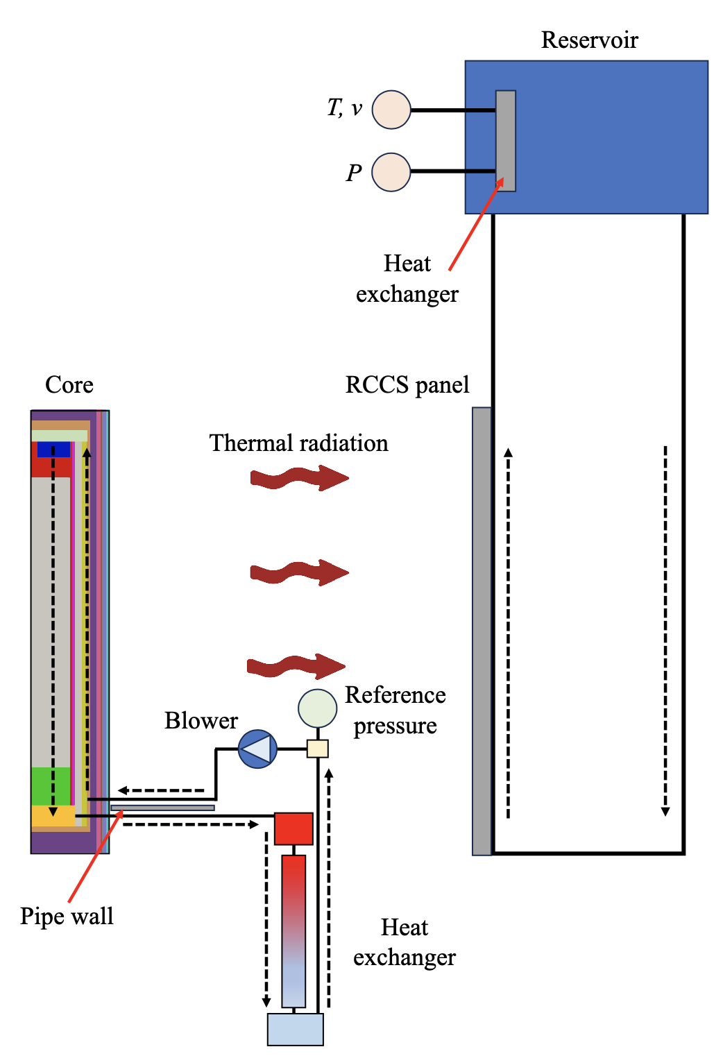
Figure 1: Schematic of the SAM HTR-PM reference plant model.
The schematic of the 2-D RZ core model is shown in Figure 2. The pebble bed, top and bottom reflectors, and the top cavity are modeled as porous media with varying porosity while the side reflectors, graphite blocks, core barrel, reactor pressure vessel (RPV), and helium gaps are modeled as solid. The hot and cold plena are not meshed in the 2-D model. Instead, they are modeled as 0-D volume branches using the SAM component system in the primary loop. On the other hand, the riser and bypass channels are modeled using an approach that utilizes both the 2-D meshes and the 1-D component system. In the 2-D model, the bypass and riser channels are meshed. However, they are treated as solid components (rather than porous media) whose thermal physical properties are reduced by a factor of . This means that in the 2-D mesh, there is no fluid flow in the riser and bypass channels. Instead, the fluid flow in these two channels are modeled as 1-D flow using PBOneDFluidComponent in the primary loop model. Conjugate heat transfer between these channels with the surrounding 2-D solid structures is also modeled. This combined approach avoids the need to mesh the two channels in the 2-D model while at the same time still captures the radial conduction of heat from the core to the surrounding reflectors.
.](../../media/htrpm_sam/htr_pm_schematics.png)
Figure 2: Schematic of the SAM 2-D RZ HTR-PM core model (Jaradat et al., 2023).
The primary loop consists of a blower, heat exchanger, and a series of flow channels. Note that the HTR-PM has a concentric channel for the inlet and outlet helium flows where the cold helium flows into the core in the outer annulus layer while the hot helium flows out of the core in the inner channel. In the primary loop model, a heat structure is added as the channel wall to model the heat transfer between the cold and hot channels. A time-dependent volume is used to provide a reference pressure of 7 MPa to the loop during steady-state normal operating condition. On the secondary side of the heat exchanger, a time-dependent junction with a velocity and temperature boundary condition is used to model the inlet while a time-dependent volume with a pressure boundary condition is used to model the outlet. The RCCS model consists of an RCCS panel, a reservoir, a heat exchanger to remove heat from the reservoir, and a series of flow channels. Heat is transferred from the RPV to the RCCS panel through thermal radiation. Flow in the RCCS loop is driven by natural circulation.
The MOOSE MultiApp system (Gaston et al., 2015) is used to couple the three models. As shown in Figure 3, the coupled model consists of one MainApp and two SubApps. The 2-D media acts as the MainApp that controls and facilitates the exchange of information between itself and the two SubApps. Inlet and outlet boundary conditions such as pressures, velocities, and temperatures are exchanged between the 2-D core and the primary loop. Furthermore, to model the conjugate heat transfer between the riser/bypass channels with the surrounding reflectors, fluid temperatures and heat transfer coefficients are transferred from the primary loop model to the 2-D model while the wall temperature from the 2-D model is transferred to the primary loop model. Similarly, to model the heat transfer between the 2-D model and the RCCS model, radiation heat flux is transferred from the 2-D model to the RCCS model where it is set as a heat flux boundary condition on the inner surface of the RCCS panel. In return, the wall temperature of the inner surface of the RCCS panel is transferred back to the 2-D model where it is used as the for the radiative boundary condition set on the outer surface of the RPV. Picard iterations are used to ensure convergence between the models.
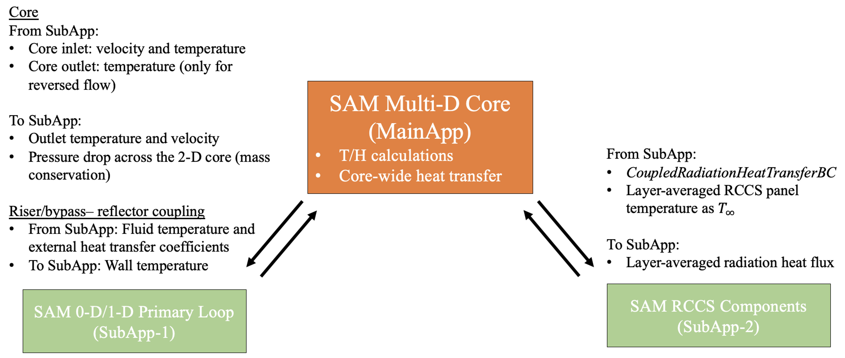
Figure 3: Coupling of the SAM models with the MultiApp system.
The domain-overlapping approach (Huxford et al., 2023) is used to accurately model the mass flow rate and pressure drop between the 2-D model and the primary loop model. A graphical representation of the approach is shown in Figure 4. In the primary loop model, the 2-D core is represented with a 1-D surrogate channel. Pressure drop across the 2-D core is calculated and transferred to the primary loop where a corresponding friction factor is calculated and imposed to the 1-D surrogate channel. In addition to the exchange of pressure drop information, by ensuring that the 2-D core and 1-D surrogate channels have the same boundary conditions at the inlet and outlet, the mass flow rate and the energy balance between the two models are conserved.
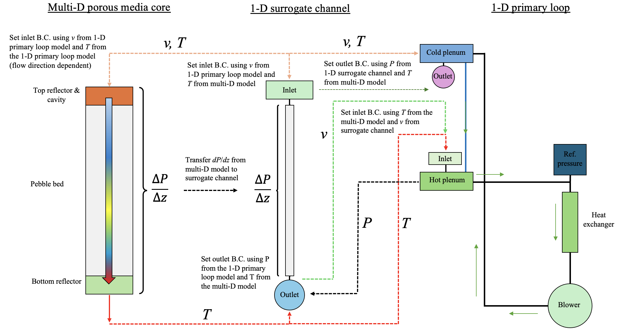
Figure 4: Domain overlapping approach used to model fluid flow.
Problem Description
Steady-state
A steady-state normal operating condition is simulated with the SAM HTR-PM reference plant model. The operating conditions during steady-state are tabulated in Figure 5. The reactor has a power output of 250 MWth and operates at 7 MPa. It is helium cooled with a system mass flow rate of 96 kg/s where the helium enters and leaves the reactor at 523.15 K and 1023.15 K, respectively. The core contains about 420,000 fuel pebbles that are 6 cm in diameter with an average packing fraction of 0.61 (Jaradat et al., 2023). In this model, neutronics calculations are not performed. Instead, a power density distribution obtained from the work by Jaradat et. al. (Jaradat et al., 2023) is imposed to the 2-D core.
.](../../media/htrpm_sam/ss-condition.png)
Figure 5: Steady-state normal operating condition of HTR-PM (Jaradat et al., 2023).
Pressurized Loss of Forced Cooling (PLOFC) Transient
The Pressurized Loss of Forced Cooling (PLOFC) transient is simulated. The sequence of events of the simulated PLOFC is shown in Figure 6. The model is first simulated until steady-state is achieved. At the start of the transient, the reactor is SCRAM and a decay heat curve is used to determine the reactor power level throughout the accident. At the same time, the helium flow rate is reduced linearly from the nominal value to zero over 13 seconds. During the accident, the pressure boundary is assumed to be intact where the system pressure is maintained at 7 MPa. Given the absence of forced flow, decay heat from the core is transferred first to the surrounding reflector, and then the graphite blocks, core barrel, and RPV. Heat is ultimately radiated from the outer surface of the RPV to the RCCS panel where it is ultimately removed by the water flow in the RCCS. Simultaneously, natural circulation is also established within the core due to density differences of helium at different elevations.
It should be pointed out that for PLOFC, a reduced primay loop model is used. Given that the pump and heat exchanger are essentially unused during the transient, they are removed to reduce the complexity of the model. Instead, an inlet boundary condition specifying the helium flow velocity and temperature is prescribed at the inlet of the riser while a pressure boundary condition is specified at the outlet of the hot plenum.
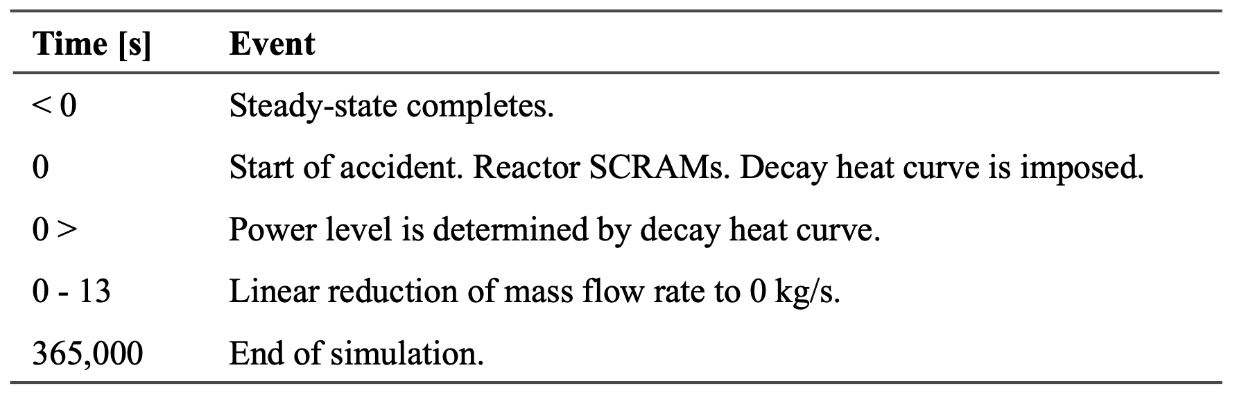
Figure 6: Sequence of events during PLOFC.
Input File Descriptions - Steady-state Normal Operating Condition
SAM uses a block-structured input syntax. Each block begins with square brackets which contain the type of input and ends with empty square brackets. Each block may contain sub-blocks. The blocks in the input file are described in the order as they appear. In the subsequent sections, input file the 2-D porous medium core model is first described, followed by the 0-D/1-D primary loop model and the RCCS model.
2-D Porous Medium Core Model
Parameters and variables that are used repeatedly in the input file are first defined. Some of these include the block names, sideset names, geometry information, boundary conditions, etc.
Global parameters
Parameters that are globally true are defined in this block. Some of these include the direction of gravity, the name of Equation of State (eos) used, and the name of parameters such as velocity (in x and y directions), pressure, temperature, and density. By doing so, users can avoid defining these parameters in the subsequent blocks where the definitions of these parameters are required. However, it should be pointed out that the global definition can be overwritten by simply defining them separately in a block. Note that the velocity in x and y directions are defined as u and v here, respectively.
[GlobalParams]
  gravity = '0 -9.807 0' # SAM default is 9.8 for Z-direction
  eos = helium
  u = vel_x
  v = vel_y
  pressure = p
  temperature = T
  rho = density

  # Reduces transfers efficiency for now, can be removed once transferred fields are checked
  bbox_factor = 10
[]
Mesh
The mesh file is specified in this block. In this model, the mesh file is in Exodus (.e) format. If R-Z coordinate is used, the direction of the vertical axis also needs to be specified.
[Mesh]
  file = htr-pm-mesh-bypass-riser.e
  coord_type = RZ
  rz_coord_axis = Y
[]
Problem
This block specifies the type of problem being solved by SAM. The type of coordinate system used in the model is also specified here. Note that if not provided, SAM assumes a Cartesian coordinate by default.
[Problem]
  type = FEProblem
[]
To restart a simulation, the location of the checkpoint file is specified with the restart_file_base parameter. The keyword LATEST is used to restart the problem from the most recent checkpoint.
restart_file_base = '<location_of_checkpoint_file>/LATEST'
Functions
Functions are defined in this block. Some examples of function types are PieceWiseLinear, CompositeFunction, and ParsedFunction. The PieceWiseLinear function is used to define the change of a parameter with respect to position or time. Below is an example of a time-dependent PieceWiseLinear function:
[Functions]
  [Q_time]
    type = PiecewiseLinear
    x = '-1.00E+06  0 1.00E-06  0.5 1 2.5 5 10  20  50  100 200 500 1000  2000  4000  6000  10000 20000 40000 60000 100000  150000  200000  250000  300000  365000 430000 495000 560000 625000 690000 755000'
    y = '1        1 0.06426 0.06193 0.06008 0.05603 0.0518  0.04704 0.04216 0.03592 0.03137 0.02739 0.02287 0.01945 0.01599 0.01281 0.01127 0.00966 0.00795 0.00655 0.00582 0.00499 0.00438 0.00399 0.00369 0.00347 0.00323 2.99e-3 2.75e-3 2.51e-3 2.27e-3 2.03e-3 1.79e-3'
  []
[]
For a position-dependent PieceWiseLinear function, the parameter axis is used to define the direction in which the position is changing.
[Functions]
  [Q_axial]
    type = PiecewiseLinear
    axis = y
    x = '3.228  3.768 4.198 4.698 5.198 5.698 6.198 6.698 7.198 7.698 8.198 8.698 9.198 10.3  11.5  12  12.8  13.4  13.8  14.228'
    y = '0.5  0.56660312  0.70174359  0.84062718  0.97604136  0.95988015   1.05950249 1.0727253 1.1394942 1.19985528  1.24058574  1.24499334 1.26168557  1.26315477 1.20720129  1.14977861 1.0 0.8 0.56820578  0.5'
  []
[]
A CompositeFunction is used to combine multiple functions, as shown below:
[Functions]
  [Q_fn]
    type = CompositeFunction
    functions = 'Q_axial Q_time Q_radial'
    scale_factor = 15.87877834e6 # To give a total of 250 MWth
  []
[]
A ParsedFunction allows operation to be performed to an variable. The variable can be postprocessor outputs or other variables. The example below shows how the average temperature is calculated using the inlet and outlet temperatures obtained from two postprocessors named 2Dreceiver_temperature_in and 2Dreceiver_temperature_out.
[Functions]
  [T_reactor_in]
    type = ParsedFunction
    expression = 'T_in'
    symbol_names = 'T_in'
    symbol_values = '2Dreceiver_temperature_in'
  []

  [T_core_out]
    type = ParsedFunction
    expression = 'T_out'
    symbol_names = 'T_out'
    symbol_values = '2Dreceiver_temperature_out'
  []
[]
EOS
This block specifies the Equation of State. The user can choose from built-in fluid library for common fluids like air, nitrogen, helium, sodium, molten salts, etc. The user can also input the properties of the fluid as constants or function of temperature. This model uses a combination of constant and temperature-dependent values for helium properties:
[EOS]
  [helium]
    type = PTFunctionsEOS
    rho = rhoHe
    cp = 5240
    mu = muHe
    k = kHe
    T_min = 500
    T_max = 1500
  []
[]
MaterialProperties
Material properties are input in this block. The values can be constants or temperature dependent as defined in the Functions block. In this model, constant material properties are used
[MaterialProperties]
  [rpv-ss-mat]
    type = HeatConductionMaterialProps
    k = 38.0
    Cp = 540.0
    rho = 7800.0
  []
  [cb-ss-mat]
    type = HeatConductionMaterialProps
    k = 17.0
    Cp = 540.0
    rho = 7800.0
  []
  [graphite]
    type = HeatConductionMaterialProps
    k = 26.0
    rho = 1780
    Cp = 1697
  []
  [he]
    type = HeatConductionMaterialProps
    k = 4
    rho = 6.0
    Cp = 5000
  []
  [graphite_porous]
    type = HeatConductionMaterialProps
    k = 17.68
    rho = 1153.96
    Cp = 1210.4
  []
[]
Variables
This block is used to input the variables in the model, namely velocities in the and (or and ) directions, pressure, fluid temperature, and solid temperature, with each variable defined in an individual sub-block. In the sub-block, the scaling factor and initial condition are defined for each variable. Additionally, the block parameter is used to specify the block names at which the variable exists. For instance, fluid temperature is only defined in the fluid blocks and not solid blocks.
[Variables]
  # Velocity
  [vel_x]
    scaling = 1e-3
    initial_condition = 1.0E-08
    block = ${fluid_blocks}
  []
  [vel_y]
    scaling = 1e-3
    initial_condition = 1.0E-08
    block = ${fluid_blocks}
  []
  # Pressure
  [p]
    scaling = 1
    initial_condition = ${p_outlet}
    block = ${fluid_blocks}
  []
  # Fluid Temperature
  [T]
    scaling = 1.0e-6
    initial_condition = ${T_inlet}
    block = ${fluid_blocks}
  []
  # Solid temperature
  [Ts]
    scaling = 1.0e-6
    initial_condition = ${T_inlet}
    block = '${pebble_blocks} ${porous_blocks} ${solid_blocks} ${cavity_blocks}'
  []
[]
AuxVariables
This block is used to input auxiliary variables, which are used to compute or store intermediate quantities that are not the main variables (the ones being solved for) of the equation system. Similar to Variables, initial condition and block can be specified for AuxVariables. Users can also set the order and family of the AuxVariables to fit their needs. For instance, porosity is defined as an AuxVariable with a CONSTANT order and a MONOMIAL family.
[AuxVariables]
  [density]
    block = ${fluid_blocks}
    initial_condition = ${rho_in}
  []
  [porosity_aux]
    order = CONSTANT
    family = MONOMIAL
  []
  [power_density]
    order = CONSTANT
    family = MONOMIAL
    initial_condition = 3.215251376e6
    block = '${active_core_blocks}'
  []
  [v_mag]
    initial_condition = ${v_mag}
    block = ${fluid_blocks}
  []

  # Aux variables for heat transfer between bypass and riser
  [T_fluid_external_bypass]
    family = LAGRANGE
    order = FIRST
    initial_condition = ${T_inlet}
  []
  [htc_external_bypass]
    family = LAGRANGE
    order = FIRST
    initial_condition = 3.0e3
  []
  [T_fluid_external_riser]
    family = LAGRANGE
    order = FIRST
    initial_condition = ${T_inlet}
  []
  [htc_external_riser]
    family = LAGRANGE
    order = FIRST
    initial_condition = 3.0e3
  []

  # Aux variables for RCCS MultiApp transfer
  [TRad]
    initial_condition = ${T_inlet}
    block = 'rpv'
  []
[]
Materials
This block is used to set material properties of solid and porous blocks using the input from the MaterialProperties block defined earlier. For components where heat conduction is modeled, SAMHeatConductionMaterial is used such as:
[Materials]
  [pebble_mat]
    type = SAMHeatConductionMaterial
    block = ${pebble_blocks}
    properties = graphite
    temperature = Ts
  []

  [graphite_mat]
    type = SAMHeatConductionMaterial
    block = 'side_reflector carbon_brick bypass_riser_reflector bypass_pebble_reflector'
    properties = graphite
    temperature = Ts
  []

  [graphite_porous_mat]
    type = SAMHeatConductionMaterial
    block = 'bypass riser'
    properties = graphite_porous
    temperature = Ts
  []

  [core_barrel_steel_mat]
    type = SAMHeatConductionMaterial
    block = 'core_barrel'
    properties = cb-ss-mat
    temperature = Ts
  []

  [rpv_steel_mat]
    type = SAMHeatConductionMaterial
    block = 'rpv'
    properties = rpv-ss-mat
    temperature = Ts
  []

  [He_gap_mat]
    type = SAMHeatConductionMaterial
    block = 'refl_barrel_gap barrel_rpv_gap'
    properties = he
    temperature = Ts
  []
[]
For porous region where convection is modeled, PorousFluidMaterial is used, as shown below. The correlations used for computing heat transfer and frictional pressure drop coefficients are specified here along with other pebble geometry information.
[Materials]
  [pebble_bed]
    type = PorousFluidMaterial
    block = ${fluid_blocks}
    d_pebble = ${pebble_diam}
    d_bed = ${pbed_d}
    porosity = porosity_aux
    friction_model = KTA
    HTC_model = KTA
    Wall_HTC_model = Achenbach
    compute_turbulence_viscosity = true
    mixing_length = 0.2
  []
[]
Heat transfer in the pebble bed is a complex phenomenon that involves pebble-pebble conduction, pebble-fluid convection, and pebble-pebble radiation. For simplicity, an effective thermal conductivity, , is often used to model these heat transfer mechanisms rather than modeling them individually. One widely used correlation to compute is the ZBS correlation (OECDNEA, 2013). In SAM, is defined using PebbleBedEffectiveThermalConductivity as shown below:
[Materials]
  [pebble_keff]
    type = PebbleBedEffectiveThermalConductivity
    block = '${pebble_blocks} ${porous_blocks} ${cavity_blocks}'
    d_pebble = ${pebble_diam}
    porosity = porosity_aux
    k_effective_model = ZBS
    solid = graphite
    tsolid = Ts
  []
[]
Kernels
The block is used to define the physics of the model. In SAM, the governing equations are essentially divided into the time derivative and spatial terms. The mass equation is modeled using PINSFEFluidPressureTimeDerivative and MDFluidMassKernel as below:
[Kernels]
  [mass_time]
    type = PINSFEFluidPressureTimeDerivative
    variable = p
    porosity = porosity_aux
    block = ${fluid_blocks}
  []

  [mass_space]
    type = INSFEFluidMassKernel
    variable = p
    porosity = porosity_aux
    block = ${fluid_blocks}
  []
[]
The and momentum terms are modeled with PINSFEFluidVelocityTimeDerivative and MDFluidMomentumKernel. Note that the component parameter in MDFluidMomentumKernel is defined as 0 and 1 for and momentum, respectively.
[Kernels]
  [mass_time]
    type = PINSFEFluidPressureTimeDerivative
    variable = p
    porosity = porosity_aux
    block = ${fluid_blocks}
  []

  [x_momentum_time]
    type = PINSFEFluidVelocityTimeDerivative
    variable = vel_x
    block = ${fluid_blocks}
  []

  [x_momentum_space]
    type = INSFEFluidMomentumKernel
    variable = vel_x
    porosity = porosity_aux
    component = 0
    block = ${fluid_blocks}
  []

  [y_momentum_time]
    type = PINSFEFluidVelocityTimeDerivative
    variable = vel_y
    block = ${fluid_blocks}
  []

  [y_momentum_space]
    type = INSFEFluidMomentumKernel
    variable = vel_y
    porosity = porosity_aux
    component = 1
    block = ${fluid_blocks}
  []
[]
Fluid energy is modeled with PINSFEFluidTemperatureTimeDerivative, MDFluidEnergyKernel, and PorousMediumEnergyKernel. The first two model the time derivative and spatial terms of the fluid heat transfer equation while the third models the heat transfer between fluid and solid.
[Kernels]
  [temperature_time]
    type = PINSFEFluidTemperatureTimeDerivative
    variable = T
    porosity = porosity_aux
    block = ${fluid_blocks}
  []

  [temperature_space]
    type = INSFEFluidEnergyKernel
    variable = T
    porosity = porosity_aux
    block = ${fluid_blocks}
  []

  [temperature_heat_transfer]
    type = PorousMediumEnergyKernel
    block = '${pebble_blocks} ${porous_blocks} ${cavity_blocks}'
    variable = T
    T_solid = Ts
  []
[]
Pebble heat transfer is modeled with PMSolidTemperatureTimeDerivative and PMSolidTemperatureKernel. For region with heat generation, the power_density_var term is set to the name of the AuxVariable for power density.
[Kernels]
  [solid_time]
    type = PMSolidTemperatureTimeDerivative
    # block = ${fluid_blocks
    block = '${pebble_blocks} ${porous_blocks} ${cavity_blocks}'
    variable = Ts
    porosity = porosity_aux
    solid = graphite
  []

  [solid_conduction]
    type = PMSolidTemperatureKernel
    variable = Ts
    block = '${porous_blocks} ${cavity_blocks}'
    T_fluid = T
  []

  [solid_conduction_core]
    type = PMSolidTemperatureKernel
    block = ${active_core_blocks}
    variable = Ts
    T_fluid = T
    power_density_var = power_density # set power density in pebble bed
  []
[]
Heat conduction in pure solid regions is modeled with HeatConductionTimeDerivative and HeatConduction:
[Kernels]
  [transient_term_reflector]
    type = HeatConductionTimeDerivative
    variable = Ts
    block = ${solid_blocks}
  []

  [diffusion_term_reflector]
    type = HeatConduction
    variable = Ts
    block = ${solid_blocks}
  []
[]
AuxKernels
The AuxKernel system mimics the kernels system but compute values that can be defined explicitly with a known function. In SAM, density is modeled using DensityAux as:
[AuxKernels]
  [rho_aux]
    type = DensityAux
    variable = density
    block = ${fluid_blocks}
  []
[]
Porosities of different regions are also modeled using ConstantAux as:
[AuxKernels]
  [porosity_bed]
    type = ConstantAux
    variable = porosity_aux
    block = 'pebble_bed'
    value = 0.39
  []

  [porosity_reflector_top]
    type = ConstantAux
    variable = porosity_aux
    block = 'top_reflector'
    value = 0.3
  []

  [porosity_reflector_bottom]
    type = ConstantAux
    variable = porosity_aux
    block = 'bottom_reflector'
    value = 0.3
  []

  [porosity_top_cavity]
    type = ConstantAux
    variable = porosity_aux
    block = 'top_cavity'
    value = 0.99
  []
[]
Lastly, the power density is modeled using FunctionAux as:
[AuxVariables]
  [power_density]
    order = CONSTANT
    family = MONOMIAL
    initial_condition = 3.215251376e6
    block = '${active_core_blocks}'
  []
[]
BCs
This block sets the boundary conditions of the model. The inlet conditions are set using MDFluidMassBC as below where the boundary parameter is set to the inlet of the model.
[BCs]
  [BC_inlet_mass]
    type = INSFEFluidMassBC
    boundary = 'core_inlet'
    variable = p
    pressure = p
    u = vel_x
    v = vel_y
    temperature = T
    eos = helium
  []
[]
The and inlet momentum boundary conditions are set using DirichletBC and PostprocessorDirichletBC, respectively as below:
[BCs]
  [BC_inlet_x_mom]
    type = DirichletBC
    boundary = 'core_inlet'
    variable = vel_x
    value = 0
  []

  [BC_inlet_y_mom]
    type = PostprocessorDirichletBC
    boundary = 'core_inlet'
    variable = vel_y
    postprocessor = 2Dreceiver_velocity_in
  []
[]
In this model, the inlet is taken as the top of the core and the inlet flow is assumed to be fully vertically downward. As a result, the momentum is set to zero at the inlet. Conversely, for the velocity (momentum), the inlet value is set to the value obtained by the 2Dreceiver_velocity_in postprocessor.
The inlet temperature is set using INSFEFluidEnergyDirichletBC as below where the out_norm parameter is used to set the outward normal of the inlet boundary or sideset.
[BCs]
  [BC_inlet_T]
    type = INSFEFluidEnergyDirichletBC
    variable = T
    boundary = 'core_inlet'
    out_norm = '0 1 0'
    T_fn = T_reactor_in
  []
[]
At the outlet of the core, a pressure boundary condition is set as below using DirichletBC. Note that the value of the pressure is set at zero at outlet boundary because the EOS used in this model is incompressible (temperature dependent only), hence the value of the pressure has no effect on the simulation results.
[BCs]
  [BC_outlet_mass]
    type = DirichletBC
    boundary = 'core_outlet'
    variable = p
    value = 0
  []
[]
Additionally, a flow direction-dependent outlet temperature is set using INSFEFluidEnergyDirichletBC as below. Note that this boundary condition is only applicable if the helium flow direction is reversed. Such a reversal may happen during certain transients where forced flow is lost.
[BCs]
  [BC_outlet_T]
    type = INSFEFluidEnergyDirichletBC
    variable = T
    boundary = 'core_outlet'
    out_norm = '0 -1 0'
    T_fn = T_core_out
  []
[]
A zero flow boundary condition is set for flow in the direction at the wall as no fluid can enter or exit the wall.
[BCs]
  [BC_fluidWall_x_mom]
    type = DirichletBC
    boundary = '${slip_wall_vertical} ${slip_wall_vertical_outer}'
    variable = vel_x
    value = 0
  []
[]
The conjugate heat transfer between the walls of the bypass and riser channels in the 2-D model and the fluids in 1-D channel in the primary loop model is modeled as below. The T_infinity and htc parameters are set to AuxVariables whose values are set using the MultiApp system based on their corresponding variables in the 1-D primary loop model.
[BCs]
  [HeatTransfer_bypass_inner_wall]
    type = CoupledConvectiveHeatFluxBC
    variable = Ts
    boundary = 'bypass_wall_vertical_inner'
    T_infinity = T_fluid_external_bypass
    htc = htc_external_bypass
  []

  [HeatTransfer_riser_inner_wall]
    type = CoupledConvectiveHeatFluxBC
    variable = Ts
    boundary = 'riser_wall_vertical_inner'
    T_infinity = T_fluid_external_riser
    htc = htc_external_riser
  []
[]
The radiation heat transfer between the RPV outer surface and the RCCS panel in the 1-D RCCS model is modeled as below. In this approach, TRad is an AuxVariable that takes its value from the inner wall temperature of the RCCS panel in the 1-D RCCS model.
[BCs]
  [HeatTransfer_bypass_inner_wall]
    type = CoupledConvectiveHeatFluxBC
    variable = Ts
    boundary = 'bypass_wall_vertical_inner'
    T_infinity = T_fluid_external_bypass
    htc = htc_external_bypass
  []

  [RPV_out]
    type = CoupledRadiationHeatTransferBC
    variable = Ts
    T_external = TRad
    boundary = 'rpv_outer'
    emissivity = 0.8
    emissivity_external = 0.8
  []
[]
Postprocessors
In this block, postprocessors are set up to obtain simulation results from the model. Below are some examples of of postprocessors from the input file.
[Postprocessors]
  [2Dsource_pressure_in]
    type = SideAverageValue
    variable = p
    boundary = 'core_inlet'
  []

  [2Dsource_pressure_out]
    type = SideAverageValue
    variable = p
    boundary = 'core_outlet'
  []

  [2Dsource_temperature_in]
    type = SideAverageValue
    variable = T
    boundary = 'core_inlet'
  []

  [2Dsource_temperature_out]
    type = SideAverageValue
    variable = T
    boundary = 'core_outlet'
  []

  [2Dsource_velocity_in]
    type = SideAverageValue
    variable = vel_y
    boundary = 'core_inlet'
  []

  [2Dsource_velocity_out]
    type = SideAverageValue
    variable = vel_y #vel_y
    boundary = 'core_outlet'
  []

  [2Dreceiver_temperature_in]
    type = Receiver
    default = 523.15
  []

  [2Dreceiver_temperature_out]
    type = Receiver
  []

  [2Dreceiver_velocity_in]
    type = Receiver
  []
  [mflow_core_in]
    type = MDSideMassFluxIntegral
    boundary = 'core_inlet'
  []
  [mflow_core_out]
    type = MDSideMassFluxIntegral
    boundary = 'core_outlet'
  []

  [total_power]
    type = ElementIntegralVariablePostprocessor
    variable = power_density
    block = ${active_core_blocks}
  []
  [pebble_bed_volume]
    type = VolumePostprocessor
    block = ${pebble_blocks}
    execute_on = 'initial'
  []

  # multi D temperature
  [Tsolid_pebble_avg]
    type = ElementAverageValue
    block = 'pebble_bed'
    variable = Ts
    execute_on = 'initial timestep_end'
  []
  [Tfluid_pebble_avg]
    type = ElementAverageValue
    block = 'pebble_bed'
    variable = T
    execute_on = 'initial timestep_end'
  []
  [Tsolid_pebble_max]
    type = ElementExtremeValue
    block = 'pebble_bed'
    value_type = max
    variable = Ts
    execute_on = 'initial timestep_end'
  []
  [Tfluid_pebble_max]
    type = ElementExtremeValue
    block = 'pebble_bed'
    value_type = max
    variable = T
    execute_on = 'initial timestep_end'
  []
  [Tsolid_reflector_avg]
    type = ElementAverageValue
    block = 'side_reflector bypass_riser_reflector bypass_pebble_reflector'
    variable = Ts
    execute_on = 'initial timestep_end'
  []
  [Tsolid_reflector_max]
    type = ElementExtremeValue
    block = 'side_reflector bypass_riser_reflector bypass_pebble_reflector'
    value_type = max
    variable = Ts
    execute_on = 'initial timestep_end'
  []
  [Tsolid_brick_avg]
    type = ElementAverageValue
    block = 'carbon_brick'
    variable = Ts
    execute_on = 'initial timestep_end'
  []
  [Tsolid_brick_max]
    type = ElementExtremeValue
    block = 'carbon_brick'
    value_type = max
    variable = Ts
    execute_on = 'initial timestep_end'
  []
  [Tsolid_core_barrel_avg]
    type = ElementAverageValue
    block = 'core_barrel'
    variable = Ts
    execute_on = 'initial timestep_end'
  []
  [Tsolid_core_barrel_max]
    type = ElementExtremeValue
    block = 'core_barrel'
    value_type = max
    variable = Ts
    execute_on = 'initial timestep_end'
  []
  [Tsolid_rpv_avg]
    type = ElementAverageValue
    block = 'rpv'
    variable = Ts
    execute_on = 'initial timestep_end'
  []
  [Tsolid_rpv_max]
    type = ElementExtremeValue
    block = 'rpv'
    value_type = max
    variable = Ts
    execute_on = 'initial timestep_end'
  []

  [core_pressure_in]
    type = SideAverageValue
    variable = p
    boundary = 'core_inlet'
  []
  [core_pressure_out]
    type = SideAverageValue
    variable = p
    boundary = 'core_outlet'
  []
  [dpdz_core]
    type = ParsedPostprocessor
    expression = 'core_pressure_out / 13.9 - core_pressure_in / 13.9'
    pp_names = 'core_pressure_out core_pressure_in'
    execute_on = 'INITIAL TIMESTEP_END'
  []
[]
Furthermore, using Receiver type postprocessors, values of postprocessors from the 1-D primary loop and RCCS models can be transferred to the 2-D model, such as
[Postprocessors]
  [2Dreceiver_temperature_in]
    type = Receiver
    default = 523.15
  []
[]
MultiApps
THe MultiApp system is set up in this block. Two sub blocks are included here - one for each of the SubApps. TransientMultiApp is used here as all of the models are set up to perform transient analyses. The catch_up parameter is set to True to allow failed solves to attempt to 'catch up' using smaller timesteps.
[MultiApps]
  [primary_loop]
    type = TransientMultiApp
    input_files = 'ss-primary-loop-full.i'
    catch_up = true
    execute_on = 'TIMESTEP_END'
  []

  [rccs]
    type = TransientMultiApp
    execute_on = timestep_end
    app_type = SamApp
    input_files = 'ss-rccs-water.i'
    catch_up = true
  []
[]
Transfers
This block is used to control the transfer of information between the MainApp and the SubApps. MultiAppPostprocessorTransfer is used to transfer postprocessor values between the Apps. The example below shows the transfer of postprocessor (2Dsource_temperature_in) value in the 2-D model to another postprocessor (1Dreceiver_temperature_in) in the primary loop model.
[Transfers]
  [2Dto1D_temperature_in_transfer]
    type = MultiAppPostprocessorTransfer
    to_multi_app = primary_loop
    from_postprocessor = 2Dsource_temperature_in
    to_postprocessor = 1Dreceiver_temperature_in
  []
[]
MultiAppUserObjectTransfer is used to transfer the value of an UserObject from one App to a variable on the other App as below. The direction parameter is used to determine the direction of the data transfer, i.e. from MainApp to SubApp or the other way round where the multi_app parameter is used for setting the SubApp of choice.
[Transfers]
  [To_subApp_Twall_riser]
    type = MultiAppUserObjectTransfer
    direction = to_multiapp
    user_object = Twall_riser_inner
    variable = Twall_riser_inner_from_main
    multi_app = primary_loop
  []
[]
MultiAppGeneralFieldNearestNodeTransfer is used to directly transfer field data between the Apps based on their nodal positions:
[Transfers]
  [from_subApp_T_fluid]
    type = MultiAppGeneralFieldNearestNodeTransfer
    direction = from_multiapp
    multi_app = primary_loop
    source_variable = temperature
    variable = T_fluid_external_riser
    from_blocks = 'riser'
    to_blocks = 'bypass_riser_reflector'
    execute_on = 'TIMESTEP_END'
  []
[]
In this example, temperature is transferred from the primary loop model (SubApp) to the 2-D model (MainApp), hence, the direction is set to from_multiapp with the multi_app being the primary loop model. source_variable is used to set the variable in the SubApp that is to be transferred to the MainApp. On the other hand, variable is the name of the variable in the MainApp to receive the transferred value. Since the transfer mechanism is based on the positions of the models, there is a possibility that the wrong field data may be transferred. To avoid that, the from_blocks and to_blocks options are set to make sure that the data transfer only involves the correct blocks.
UserObjects
This UserObjects system is used to perform custom algorithms or calculations that may not fit well within any other system in MOOSE.
[UserObjects]
  [QRad_UO]
    type = LayeredSideFluxAverage
    variable = Ts
    direction = y
    num_layers = 45
    boundary = 'rpv_outer'
    diffusivity = thermal_conductivity
    execute_on = 'TIMESTEP_END'
  []

  [Twall_riser_inner]
    type = LayeredSideAverage
    direction = y
    num_layers = 36
    sample_type = direct
    variable = Ts
    boundary = 'riser_wall_vertical_inner'
  []

  [Twall_bypass_inner]
    type = LayeredSideAverage
    direction = y
    num_layers = 36
    sample_type = direct
    variable = Ts
    boundary = 'bypass_wall_vertical_inner'
  []
[]
In this model, LayeredSideAverage is used to obtain the layered average field data such as the wall temperatures on the riser and bypass channels and the radiative heat flux on the RPV outer wall. The num_layers option is used to set the number of layers over which a field data is averaged and the direction option is used to set the averaging direction.
Preconditioning
This block describes the preconditioner to be used by the preconditioned JFNK solver (available through PETSc). Two options are currently available, the single matrix preconditioner (SMP) and the finite difference preconditioner (FDP) (for debugging only). The theory behind the preconditioner can be found in the SAM Theory Manual (Hu et al., 2021). New users can leave this block unchanged.
[Preconditioning]
  [SMP_PJFNK]
    type = SMP
    full = true
    solve_type = 'PJFNK'
    petsc_options_iname = '-pc_type -ksp_gmres_restart'
    petsc_options_value = 'lu 100'
  []
[]
Executioner
This block describes the calculation process flow. The user can specify the start time, end time, time step size for the simulation. The user can also choose to use an adaptive time step size with the IterationAdaptiveDT time stepper. Other inputs in this block include PETSc solver options, convergence tolerance, quadrature for elements, etc.
[Executioner]
  type = Transient
  dtmin = 1e-6
  dtmax = 500

  [TimeStepper]
    type = IterationAdaptiveDT
    growth_factor = 1.25
    optimal_iterations = 10
    linear_iteration_ratio = 100
    dt = 0.1
    cutback_factor = 0.8
    cutback_factor_at_failure = 0.8
  []

  nl_rel_tol = 1e-5
  nl_abs_tol = 1e-4
  nl_max_its = 15
  l_tol = 1e-3
  l_max_its = 100

  start_time = -200000
  end_time = 0

  fixed_point_rel_tol = 1e-3
  fixed_point_abs_tol = 1e-3
  fixed_point_max_its = 10
  relaxation_factor = 0.8
  relaxed_variables = 'p T vel_x vel_y'
  accept_on_max_fixed_point_iteration = true

  [Quadrature]
    type = GAUSS
    order = SECOND
  []
[]
Outputs
This block is used to control the information to be output by the model. Users can choose the output format as Exodus and/or CSV files. Checkpoint files can also be produced. User can set the output frequency via the interval option.
[Outputs]
  perf_graph = true
  print_linear_residuals = false
  [out]
    type = Exodus
    use_displaced = true
    sequence = false
  []
  [csv]
    type = CSV
  []
  # Commented out for git purpose
  [checkpoint]
    type = Checkpoint
    execute_on = 'INITIAL TIMESTEP_END'
  []
  [console]
    type = Console
    fit_mode = AUTO
    execute_scalars_on = 'NONE'
  []
[]
0-D/1-D Primary Loop Model
The input file of the 0-D/1-D primary loop model is described here. Some of the blocks in this file are similar to the input file of the porous media model and will not be repeated here. These include the [GlobalParams], [Functions], [EOS], [MaterialProperties], [Postprocessors], [Preconditioning], [Executioner] and [Outputs] blocks. Instead, this section focuses on the [Components] block to describe the actual model.
As described earlier, the so-called domain overlapping approach is used to couple the multi-D porous media model to the 0-D/1-D primary loop. The primary loop model essentially consists of two parts: a surrogate channel to represent the multi-D core and a remainder of the primary loop with flow channels, pump, heat exchanger, etc.
The surrogate channel consists of a PBOneDFluidComponent with inlet and outlet boundary conditions.
[Components]
  [core_pipe]
    type = PBOneDFluidComponent
    eos = helium
    A = 7.068583471 # Based on pbed flow area in mainapp
    length = 13.9 # 15.7-1.8
    Dh = 3
    n_elems = 1
    orientation = '0 1 0'
    position = '0.845 1.8 0'
    overlap_coupled = true
    overlap_pp = dpdz_core_receive
  []
[]
The geometric information such as the length, flow area, hydraulic diameter, position, etc. are the same as that in the porous media model. In the domain overlapping approach, frictional pressure drop in the porous media model is computed and then applied to the surrogate channel. The pressure drop is then used by the code to internally calculate a friction factor that is then applied to the surrogate channel. By doing so, the flow rate in the surrogate channel is ensured to be the same as that in the porous media model. This capability is enabled by setting overlap_coupled to true. The overlap_pp parameter sets the postprocessor name that receives the pressure drop information from the porous media model. Note that pressure drop is defined as the change of pressure per unit length, , with a unit of Pa/m, and NOT the total pressure drop across the core.
The inlet and outlet boundary conditions are set using a coupled postprocessor time-dependent junction (CoupledPPSTDJ) and coupled postprocessor time-dependent volume (CoupledPPSTDV), respectively. At the inlet, the velocity and temperature boundary conditions are set to the mean values obtained from the inlet of the multi-D model using their respective postprocessors. On the other hand, at the outlet, using their respective postprocessors, the temperature is set to the mean temperature obtained at the outlet of the multi-D model while the pressure is set to the pressure of the hot plenum.
[Components]
  [coupled_inlet_top]
    type = CoupledPPSTDJ
    input = 'core_pipe(out)'
    eos = helium
    postprocessor_vbc = core_top_velocity_scaled # core_velocity
    postprocessor_Tbc = T_cold_plenum_inlet_pipe_inlet # T from cold plenum
    v_bc = -2
    T_bc = 523.15
  []

  [coupled_outlet]
    type = CoupledPPSTDV
    input = 'core_pipe(in)'
    eos = helium
    # p_bc = 7e6
    postprocessor_pbc = p_hot_plenum_inlet_pipe_outlet # p from hot_plenum_inlet_pipe outlet
    postprocessor_Tbc = T_hot_plenum_inlet_pipe_outlet # T from hot_plenum_inlet_pipe outlet
  []
[]
Other than the surrogate channel, the remainder of the primary loop is shown in Figure 1. In this model, the hot plenum can be seen as the inlet and the cold plenum the outlet. To couple the outlet of the surrogate channel to the hot plenum, the outlet conditions of the surrogate channel are used as the inlet conditions of the hot plenum. The hot plenum is modeled using the PBVolumeBranch component as:
[Components]
  [hot_plenum]
    type = PBVolumeBranch
    eos = helium
    center = '0.845 1.4 0'
    inputs = 'hot_plenum_inlet_pipe(in) bypass(out)'
    outputs = 'outlet_pipe(in)'
    K = '0.0 0.0 0.0'
    width = 0.8 # display purposes
    height = 1.69 # display purposes
    Area = 8.9727
    volume = 7.17816
  []
[]
Given that boundary conditions cannot be directly set to a PBVolumeBranch, a short pipe called the 'hot_plenum_inlet_pipe' is connected to the 'hot_plenum' on one end, while the end is set to the outlet conditions from the surrogate channel using the CoupledPPSTDJ component as:
[Components]
  [coupled_inlet]
    type = CoupledPPSTDJ
    input = 'hot_plenum_inlet_pipe(out)'
    eos = helium
    postprocessor_vbc = core_velocity_scaled #core_velocity
    postprocessor_Tbc = 1Dreceiver_temperature_out # T from 2D domain T_out
    v_bc = -2
    T_bc = 523.15
  []
[]
After the hot plenum is a horizontal flow channel known as the 'outlet_pipe':
[Components]
  [cold_plenum_outlet_pipe]
    type = PBOneDFluidComponent
    A = 7.068583471 # Based on pbed flow area in mainapp
    length = 0.1
    Dh = 3
    n_elems = 1
    orientation = '0 1 0'
    position = '1.065 15.7 0' #'0.845 1.5 0'
    eos = helium
    initial_V = -2
  []
[]
Downstream of 'outlet_pipe' is a PBVolumeBranch known as 'SG_inlet_plenum' that connects the outlet pipe to the heat exchanger:
[Components]
  [SG_inlet_plenum]
    type = PBVolumeBranch
    eos = helium
    center = '7.433 1.4 0'
    inputs = 'outlet_pipe(out)'
    outputs = 'IHX(primary_in)'
    K = '0.0 0.0'
    height = 2.598 # display purposes
    width = 3.031 # display purposes
    Area = 5.3011265
    volume = 16.0677
  []
[]
The heat exchanger is intended to represent the steam generator in the actual HTR-PM reactor. The geometries of the heat exchanger used in this work are obtained from publicly available information:
[Components]
  [IHX]
    type = PBHeatExchanger
    HX_type = Countercurrent
    eos_secondary = water
    position = '7.433 1.4 0'
    orientation = '0 -1 0'
    A = 7.618966942
    Dh = 1
    PoD = 1.5789 # 30 mm /19 mm
    HTC_geometry_type = Bundle
    length = 7.75
    n_elems = 20
    HT_surface_area_density = 65.99339913 # back calculated from secondary flow area and Aw #3.32344752
    A_secondary = 1.141431617
    Dh_secondary = 1
    length_secondary = 7.75
    HT_surface_area_density_secondary = 421.0526316
    hs_type = cylinder
    radius_i = 0.009080574
    wall_thickness = 0.000419426
    n_wall_elems = 3
    material_wall = ss-mat
    Twall_init = ${T_inlet}
    initial_T_secondary = ${T_inlet}
    initial_P_secondary = ${p_secondary}
    initial_V_secondary = '${fparse -v_secondary}'
    SC_HTC = 2.5 # approximation for twisted tube effect
    SC_HTC_secondary = 2.5
    disp_mode = -1
  []
[]
Water is used as the coolant on the secondary side of the heat exchanger. For simplicity, the secondary side is not modeled and is simply given inlet and outlet boundary conditions:
[Components]
  [IHX2-in]
    type = PBTDJ
    v_bc = '${fparse -v_secondary}'
    T_bc = ${T_in_secondary}
    eos = water
    input = 'IHX(secondary_in)'
  []

  [IHX2-out]
    type = PBTDV
    eos = water
    p_bc = ${p_secondary}
    input = 'IHX(secondary_out)'
  []
[]
Similar to the inlet, the outlet of the heat exchanger is connected to a PBVolumeBranch component:
[Components]
  [SG_outlet_plenum]
    type = PBVolumeBranch
    eos = helium
    center = '7.433 -6.35 0'
    inputs = 'IHX(primary_out)'
    outputs = 'SG_outlet_pipe(in)'
    K = '0.0 0.0'
    height = 1.732 # display purposes
    width = 1.732 # display purposes
    Area = 2.356056
    volume = 10.881838
  []
[]
Downstream of the heat exchanger is another flow channel that connects the outlet of the heat exchanger to the inlet of the blower:
[Components]
  [SG_outlet_pipe]
    type = PBOneDFluidComponent
    A = 2.2242476
    Dh = 0.4
    length = 12.745
    n_elems = 20
    orientation = '0 1 0'
    position = '8.299 -6.35 0'
  []
[]
The outlet of 'SG_outlet_pipe' is connected to the blower through a PBVolumeBranch:
[Components]
  [pump_inlet_plenum]
    type = PBVolumeBranch
    eos = helium
    center = '8.299 6.395 0'
    inputs = 'SG_outlet_pipe(out)'
    outputs = 'pump_inlet_pipe(in) ref_pressure_pipe(in)'
    K = '0.0 0.0 0.0'
    height = 0.7575 # display purposes
    width = 3.928 # display purposes
    Area = 12.118
    volume = 18.3588
  []
[]
Additionally, the reference pressure of the system is set using a PBTDV component that is connected to 'pump_inlet_plenum'. During steady-state, the system pressre is set to 7 MPa.
[Components]
  [ref_pressure_pipe]
    type = PBOneDFluidComponent
    A = 2.2242476
    Dh = 0.4
    length = 1
    n_elems = 5
    orientation = '1 0 0'
    position = '8.299 6.395 0'
  []

  [reference_pressure]
    type = PBTDV
    eos = helium
    p_fn = p_out_fn
    input = 'ref_pressure_pipe(out)'
  []
[]
Downstream of that is a flow channel that connects the PBVolumeBranch to the blower:
[Components]
  [pump_inlet_pipe]
    type = PBOneDFluidComponent
    A = 2.2242476
    Dh = 0.4
    length = 1.135
    n_elems = 20
    orientation = '-1 0 0'
    position = '8.299 6.395 0'
  []
[]
The blower is modeled using the PBPump component. Note that the pump head is set using the 'f_pump_head' function via the Head_fn parameter. The pump head and the k-loss values are tuned such that the steady-state mass flow rate is 96 kg/s.
[Components]
  [blower]
    type = PBPump
    inputs = 'pump_inlet_pipe(out)'
    outputs = 'pump_outlet_pipe(in)'
    K = '7500 7500'
    K_reverse = '7500 7500'
    Area = 2.2242476
    Head = f_pump_head
  []
[]
Located downstream of the blower are a pipe and a PBVolumeBranch that is connected to the horizontal inlet pipe:
[Components]
  [pump_outlet_pipe]
    type = PBOneDFluidComponent
    A = 2.2242476
    Dh = 0.4
    length = 4.34781
    n_elems = 20
    orientation = '0 -1 0'
    position = '7.164 6.395 0'
  []

  [pump_outlet_branch]
    type = PBVolumeBranch
    eos = helium
    center = '7.164 2.04719 0'
    inputs = 'pump_outlet_pipe(out)'
    outputs = 'inlet_pipe(in)'
    K = '0.0 0.0'
    width = 0.05 # display purposes
    height = 0.05 # display purposes
    Area = 2.2242476
    volume = 0.01
  []

  [hot_plenum_inlet_pipe]
    type = PBOneDFluidComponent
    A = 7.068583471 # Based on pbed flow area in mainapp
    length = 0.5
    Dh = 3
    n_elems = 1
    orientation = '0 1 0'
    position = '0.845 1.3 0' #'1.065 15.85 0'
  []
[]
The outlet of the horizontal inlet pipe is connected to the inlet of the riser. In order to accurately account for the heat transfer between the 2-D surfaces and the riser, the heat transfer area density is set via the HT_surface_area_density parameter.
[Components]
  [riser]
    type = PBOneDFluidComponent
    A = 0.81631
    Dh = 0.2
    length = 13.65281 #
    n_elems = 20
    orientation = '0 1 0'
    position = '2.03 2.04719 0'
    HT_surface_area_density = 14.85532
  []

  [joint_outlet_1]
    type = PBSingleJunction
    eos = helium
    inputs = 'inlet_pipe(out)'
    outputs = 'riser(in)'
  []
[]
The outlet of the riser is connected to the cold plenum:
[Components]
  [cold_plenum]
    type = PBVolumeBranch
    eos = helium
    center = '1.065 15.85 0'
    inputs = 'riser(out)'
    outputs = 'bypass(in) cold_plenum_outlet_pipe(out)'
    K = '0.0 0.0 0.0'
    width = 0.8 # display purposes
    height = 1.69 # display purposes
    Area = 8.9727
    volume = 7.17816
  []
[]
A bypass channel connects the cold and hot plena. Similar to the riser, the heat transfer area density of the bypass channel is set to accurately capture the heat transfer between the helium in the bypass channel and the surrounding 2-D solid structures. A friction factor, f, is tuned such that the flow in the bypass channel is roughly 1 kg/s:
[Components]
  [bypass]
    type = PBOneDFluidComponent
    A = 0.42474
    length = 13.9
    Dh = 0.13
    n_elems = 20
    orientation = '0 -1 0'
    position = '1.625 15.7 0'
    HT_surface_area_density = 23.077
    f = 2000
  []
[]
The cold plenum can be seen as the outlet of the primary loop. Similar to the hot plenum, a small pipe is connected to the cold plenum on one end where the boundary conditions are set on the other end using the CoupledPPSTDV component. The outlet pressure is set to the pressure at the outlet of the surrogate channel while the temperature is set to the mean temperature at the inlet of the 2-D core:
[Components]
  [cold_plenum_outlet_pipe]
    type = PBOneDFluidComponent
    A = 7.068583471 # Based on pbed flow area in mainapp
    length = 0.1
    Dh = 3
    n_elems = 1
    orientation = '0 1 0'
    position = '1.065 15.7 0' #'0.845 1.5 0'
    eos = helium
    initial_V = -2
  []

  [coupled_outlet_top]
    type = CoupledPPSTDV
    input = 'cold_plenum_outlet_pipe(in)'
    eos = helium
    postprocessor_pbc = p_core_pipe_outlet
    postprocessor_Tbc = 1Dreceiver_temperature_in
  []
[]
The wall separating the horizontal inlet and outlet pipes is modeled using a PBCoupledHeatStructure. The boundary conditions both sides of the wall are set to Coupled to model the heat transfer between the helium in the inlet and outlet pipe across the wall.
[Components]
  [concentric-pipe-wall]
    type = PBCoupledHeatStructure
    position = '7.164 0 0'
    orientation = '-1 0 0'
    hs_type = cylinder

    length = 5.134
    width_of_hs = '0.10951'
    radius_i = 1.7873
    elem_number_radial = 3
    elem_number_axial = 20
    dim_hs = 2
    material_hs = 'ss-mat'
    Ts_init = ${T_inlet}

    HS_BC_type = 'Coupled Coupled'
    name_comp_left = outlet_pipe
    HT_surface_area_density_left = 5.177314
    name_comp_right = inlet_pipe
    HT_surface_area_density_right = 1.2413889 # PI * D / A(pipe1)
  []
[]
The HeatTransferWithExternalHeatStructure is used to model the heat transfer between the solids in the multi-D model and the 1-D bypass and riser channels in the primary loop model. In this approach, the wall temperatures from the 2-D model are transferred to 1-D channels. In return, the 2-D walls receive the fluid temperatures and the heat transfer coefficients from the 1-D channels. The T_wall_name is the variable name to which the MultiApp transfers the wall temperatures from the multi-D model.
[Components]
  [from_main_app_riser]
    type = HeatTransferWithExternalHeatStructure
    flow_component = riser
    initial_T_wall = ${T_inlet}
    T_wall_name = Twall_riser_inner_from_main
  []

  [from_main_app_bypass]
    type = HeatTransferWithExternalHeatStructure
    flow_component = bypass
    initial_T_wall = ${T_inlet}
    T_wall_name = Twall_bypass_inner_from_main
  []
[]
0-D/1-D RCCS Model
The input file of the 0-D/1-D model is described here. Similarly, blocks that are repeated in other input files will not be discussed here. Note that the RCCS model is loosely based on the actual system whose information is obtained from multiple sources in the public domain and the geometry information is not representative of the actual system.
The RCCS panel in the model receives heat flux from the outer surface of the RPV in the multi-D porous media model via thermal radiation. To do so, an AuxVariable named 'QRad' is defined to receive that flux. Note that the name of the AuxVariable ('QRad' in this case) must match the name provided in the [QRad_to_subRCCS] block in the multi-D model. At the same time, due to the difference in the surface area of the RPV and the RCCS panel, the heat flux needs to be properly scaled to ensure energy conservation. This is done through another AuxVariable named 'QRad_multiplied'.
[AuxVariables]
  [QRad]
    block = 'rccs-panel:hs0'
  []
  [QRad_multiplied]
    block = 'rccs-panel:hs0'
  []
[]
The scaling of the heat flux is performed through an AuxKernel of type ParsedAux. The scaling factor is defined as the ratio between the RPV surface area to the RCCS panel surface area.
[AuxKernels]
  [QRad_multiplied]
    type = ParsedAux
    block = 'rccs-panel:hs0'
    variable = QRad_multiplied
    coupled_variables = 'QRad'
    expression = 'QRad * 18.84955592 / 26.452210 ' #  Multiplier = (2 * PI * r_rpv_outer) / (2 * PI * r_rccs_panel_inner) --> Qrad_rpv * area_rpv = Qrad_rccs * area_rccs_inner
    execute_on = 'timestep_end'
  []
[]
In return, the multi-D porous media model receives a layer-averaged wall temperature from the surface of the RCCS and imposes that as the of the radiative boundary condition imposed on the RPV outer surface. The layer-averaging is done through a UserObjects of type LayeredSideAverage. Note that the same of the UserObject, 'TRad_UO' must match the user_object name provided in the [TRad_from_RCCS_sub] block in the multi-D model.
[UserObjects]
  [TRad_UO]
    type = LayeredSideAverage
    variable = T_solid
    direction = y
    num_layers = 45
    boundary = 'rccs-panel:inner_wall'
    execute_on = 'timestep_end'
    use_displaced_mesh = true
  []
[]
The components of the RCCS model are modeled in the [Components] block in the input file. The RCCS panel is modeled as a PBCoupledHeatStructure with a 'Convective' boundary condition on the inner surface and a 'Coupled' boundary condition on the outer surface. The scaled heat flux, 'QRad_multiplied' is applied to the inner surface through the qs_external_left parameter. On the other hand, the outer surface is coupled to a fluid component named 'rccs-heated-riser' via the name_comp_right parameter. The heat transfer surface area density on the right side is provided through the HT_surface_area_density_right parameter.
[Components]
  [rccs-panel]
    type = PBCoupledHeatStructure
    position = '0 0 0.0'
    orientation = '0 1 0'
    hs_type = cylinder

    length = 16.8
    width_of_hs = '0.1'
    radius_i = 4.21
    elem_number_radial = 5
    elem_number_axial = 50
    dim_hs = 2
    material_hs = 'ss-mat'
    Ts_init = ${T_inlet_rccs}

    HS_BC_type = 'Convective Coupled'
    qs_external_left = QRad_multiplied
    name_comp_right = rccs-heated-riser
    HT_surface_area_density_right = 158.748 #1.525027801   # PI * D / A(pipe1)
  []
[]
The riser is coupled to the outer surface of the RCCS panel. Downstream of the riser is an unheated chimney. The chimney is assumed to be fairly tall to provide sufficient thermal driving head for natural circulation.
[Components]
  [rccs-heated-riser]
    type = PBOneDFluidComponent
    A = 0.170588 #17.7574
    Dh = ${Dh_pipe} #0.031655 # From Roberto et al (2020)'s paper using total flow area and pipe number
    length = 16.8
    n_elems = 50
    orientation = '0 1 0'
    position = '4.31 0 0'
  []

  [rccs-chimney]
    type = PBOneDFluidComponent
    A = 0.170588 #17.7574
    Dh = ${Dh_pipe}
    length = 10
    n_elems = 50
    orientation = '0 1 0'
    position = '4.31 16.8 0'
  []
[]
The outlet of the chimney is connected to a reservoir/pool that is modeled using a PBLiquidVolume component with an initial level of 10 m. The pool is assumed to be at atmospheric pressure.
[Components]
  [pool]
    type = PBLiquidVolume
    center = '4.81 29.3 0'
    outputs = 'rccs-chimney(out) rccs-downcomer(out) IHX-inlet-pipe(in) IHX-outlet-pipe(out)'
    K = '0 0 0 0'
    orientation = '0 1 0'
    Area = 30
    volume = 300

    initial_T = 303 #${T_inlet}
    initial_level = 10 # 5
    ambient_pressure = 1.01325e5
    eos = eos
    width = 1
    height = 5
  []
[]
A heat exchanger is used in the pool for decay heat removal. On the primary side, the inlet and outlet of the heat exchanger are connected to the pool while a time-dependent junction and volume are used at the inlet and outlet on the seconday side. Water enters the secondary side at 303 K. Note that a large inlet flow rate is set on the secondary side to ensure to provide sufficient cooling to the pool.
[Components]
  [IHX]
    type = PBHeatExchanger
    HX_type = Countercurrent
    eos_secondary = eos
    position = '4.81 31.8 0'
    orientation = '0 -1 0'
    A = 0.36571
    Dh = 0.0108906
    PoD = 1.17
    HTC_geometry_type = Bundle
    length = 5
    n_elems = 10
    HT_surface_area_density = 734.582
    A_secondary = 0.603437
    Dh_secondary = 0.0196
    length_secondary = 5
    HT_surface_area_density_secondary = 408.166
    hs_type = cylinder
    radius_i = 0.0098
    wall_thickness = 0.000889
    n_wall_elems = 3
    material_wall = ss-mat
    Twall_init = 303
    initial_T_secondary = 303
    initial_P_secondary = 1e5
    initial_V_secondary = -100
    SC_HTC = 2.5
    SC_HTC_secondary = 2.5
    disp_mode = -1
    eos = eos
  []

  [IHX-inlet-pipe]
    type = PBOneDFluidComponent
    input_parameters = CoolantChannel
    position = '4.81 29.3 -1'
    orientation = '0 0 1'
    length = 1
    A = 0.170588481 # Assume 1 cm wide from r = 2.71 to 2.72
    Dh = 2
    HTC_geometry_type = Pipe
    n_elems = 10
    eos = eos
    initial_T = 303
  []

  [IHX-outlet-pipe]
    type = PBOneDFluidComponent
    input_parameters = CoolantChannel
    position = '4.81 26.8 0'
    orientation = '0 0 -1'
    length = 1
    A = 0.170588481 # Assume 1 cm wide from r = 2.71 to 2.72
    Dh = 2
    HTC_geometry_type = Pipe
    n_elems = 10
    eos = eos
    initial_T = 303
  []

  [IHX-junc-out]
    type = PBSingleJunction
    eos = eos
    inputs = 'IHX(primary_out)'
    outputs = 'IHX-outlet-pipe(in)'
    initial_T = 303
  []

  [IHX-junc-in]
    type = PBVolumeBranch
    center = '2.72 27.8 6'
    inputs = 'IHX-inlet-pipe(out)'
    outputs = 'IHX(primary_in)'
    K = '0 0'
    Area = 0.170588481
    volume = 0.01
    width = 0.02049
    height = 0.3
    eos = eos
  []

  [IHX2-in]
    type = PBTDJ
    v_bc = -100
    T_bc = 303
    eos = eos
    input = 'IHX(secondary_in)'
  []

  [IHX2-out]
    type = PBTDV
    eos = eos
    p_bc = 1e5
    input = 'IHX(secondary_out)'
  []
[]
Downstream of the pool is the downcomer consisting of a vertical and horizontal section. The outlet of the horizontal section is connected to the inlet of the riser, thus completing the loop.
[Components]
  [rccs-downcomer]
    type = PBOneDFluidComponent
    A = 0.170588 #17.7574
    Dh = ${Dh_pipe}
    length = 26.8
    n_elems = 50
    orientation = '0 1 0'
    position = '5.31 0 0'
  []

  [rccs-downcomer-horizontal]
    type = PBOneDFluidComponent
    A = 0.170588 #17.7574
    Dh = ${Dh_pipe}
    length = 1
    n_elems = 5
    orientation = '1 0 0'
    position = '4.31 0 0'
  []
[]
The flow channels are connected to each other with PBVolumeBranch.
[Components]
  [junc-riser-chimney]
    type = PBVolumeBranch
    eos = eos
    inputs = 'rccs-heated-riser(out)'
    outputs = 'rccs-chimney(in)'
    K = '0 0'
    Area = 0.170588 #17.7574
    center = '4.31 16.8 0'
    volume = 0.01
  []

  [junc-horizontal-riser]
    type = PBVolumeBranch
    eos = eos
    inputs = 'rccs-downcomer-horizontal(out)'
    outputs = 'rccs-heated-riser(in)'
    K = '0 0'
    Area = 0.170588 #17.7574
    center = '4.31 0 0'
    volume = 0.01
  []

  [junc-downcomer-horizontal]
    type = PBVolumeBranch
    eos = eos
    inputs = 'rccs-downcomer(in)'
    outputs = 'rccs-downcomer-horizontal(in)'
    K = '0 0'
    Area = 0.170588 #17.7574
    center = '5.31 0 0'
    volume = 0.01
  []
[]
Input File Descriptions - Pressurized Loss of Forced Cooling (PLOFC) Transient
The transient PLOFC simulation is a restart from the steady-state simulation with some minor modifications in the input files. As mentioned earlier, a simplified primary loop model is used in the PLOFC simulation. As a result, the full coupled model needs to be re-run with the simplified primary loop in lieu of the full primary loop model whose output is then used to restart the PLOFC simulation. The [Problem] block in all three input files are modified where the path of the restart file is specified using the restart_file_base parameter. The LATEST keyword is used to specify the latest checkpoint as the restart time stamp. Alternatively, the restart time stamp can be set to another time step by specifying the time-step number.
[Problem]
  type = FEProblem
  restart_file_base = 'ss-main_checkpoint_cp/450'
  # restart_file_base = 'ss-main_checkpoint_cp/LATEST'
[]
[Problem]
  restart_file_base = 'ss-main_out_primary_loop0_checkpoint_cp/450'
  # restart_file_base = 'ss-main_out_primary_loop0_checkpoint_cp/LATEST'
[]
[Problem]
  restart_file_base = 'ss-main_out_rccs0_checkpoint_cp/450'
  # restart_file_base = 'ss-main_out_rccs0_checkpoint_cp/LATEST'
[]
The SubApp files in the [MultiApps] block are changed to the transient files
[MultiApps]
  [primary_loop]
    type = TransientMultiApp
    input_files = 'plofc-primary-loop-transient.i'
    catch_up = true
    execute_on = 'TIMESTEP_END'
  []

  [rccs]
    type = TransientMultiApp
    execute_on = timestep_end
    app_type = SamApp
    input_files = 'plofc-rccs-water-transient.i'
    catch_up = true
  []
[]
Furthermore, the start_time and end_time parameters in the [Executioner] blocks of all three input files are modified to the desired values.
In the multi-D input file, the initial_condition parameters in the [Variables] and [AuxVariables] are removed.
Lastly, as discussed previously, the primary loop is simplified where components such as the blower, heat exchanger, and reference pressures are removed and replaced with inlet and outlet boundary conditions. Note that in the [inlet] block, the mass flow rate is set using the m_fn user-defined function.
[Components]
  [coupled_inlet]
    type = CoupledPPSTDJ
    input = 'hot_plenum_inlet_pipe(out)'
    eos = helium
    postprocessor_vbc = core_velocity_scaled #core_velocity
    postprocessor_Tbc = 1Dreceiver_temperature_out # T from 2D domain T_out
    v_bc = -2
    T_bc = 523.15
  []

  [coupled_outlet]
    type = CoupledPPSTDV
    input = 'core_pipe(in)'
    eos = helium
    # p_bc = 7e6
    postprocessor_pbc = p_hot_plenum_inlet_pipe_outlet # p from hot_plenum_inlet_pipe outlet
    postprocessor_Tbc = T_hot_plenum_inlet_pipe_outlet # T from hot_plenum_inlet_pipe outlet
  []
[]
Running the Simulation
SAM can be run on Linux, Unix, and MacOS. Due to its dependence on MOOSE, SAM is not compatible with Windows. Given that this is a MultiApp simulation, only the MainApp, i.e. ss-main.i needs to be run. The SubApps will be called and executed automatically by the MainApp. The model can be run from the shell prompt as shown below using SAM
sam-opt -i ss-main.i
With Blue Crab, the model can be run as below where the flag --app is used to specify SAM as the running application
blue_crab-opt -i ss-main.i --app SamApp
Similarly, for running the transient simulation with SAM
sam-opt -i plofc-main-transient.i
And with Blue Crab
blue_crab-opt -i plofc-main-transient.i --app SamApp
Acknowledgements
This report was prepared as an account of work sponsored by an agency of the U.S. Government. Neither the U.S. Government nor any agency thereof, nor any of their employees, makes any warranty, expressed or implied, or assumes any legal liability or responsibility for any third party’s use, or the results of such use, of any information, apparatus, product, or process disclosed in this report, or represents that its use by such third party would not infringe privately owned rights. The views expressed in this paper are not necessarily those of the U.S. Nuclear Regulatory Commission. This work is supported by the U.S. Nuclear Regulatory Commission, under Task Order Agreement No. 31310021F0005. The authors would like to acknowledge the support and assistance from Dr. Mustafa Jaradat, Dr. Sebastian Schunert, and Dr. Javier Ortensi of Idaho National Laboratory in the completion of this work.
References
- Derek R. Gaston, Cody J. Permann, John W. Peterson, Andrew E. Slaughter, David Andrš, Yaqi Wang, Michael P. Short, Danielle M. Perez, Michael R. Tonks, Javier Ortensi, Ling Zou, and Richard C. Martineau.
Physics-based multiscale coupling for full core nuclear reactor simulation.
Annals of Nuclear Energy, 84:45–54, 2015.[BibTeX]
@article{multiapp_gaston2015, author = "Gaston, Derek R. and Permann, Cody J. and Peterson, John W. and Slaughter, Andrew E. and Andr{\v{s}}, David and Wang, Yaqi and Short, Michael P. and Perez, Danielle M. and Tonks, Michael R. and Ortensi, Javier and Zou, Ling and Martineau, Richard C.", title = "Physics-based multiscale coupling for full core nuclear reactor simulation", year = "2015", journal = "Annals of Nuclear Energy", volume = "84", pages = "45--54", publisher = "Elsevier" } - R. Hu, L. Zou, G. Hu, D. Nunez, T. Mui, and T. Fei.
SAM Theory Manual.
Technical Report ANL/NE-17/4 Rev. 1, Argonne National Laboratory, Lemont, IL, 2021.[BibTeX]
@techreport{Hu2021, author = "Hu, R. and Zou, L. and Hu, G. and Nunez, D. and Mui, T. and Fei, T.", address = "Lemont, IL", number = "ANL/NE-17/4 Rev. 1", institution = "Argonne National Laboratory", title = "{SAM Theory Manual}", year = "2021" } - Aaron Huxford, Victor Coppo Leite, Elia Merzari, Ling Zou, Victor Petrov, and Annalisa Manera.
A hybrid domain overlapping method for coupling system thermal hydraulics and cfd codes.
Annals of Nuclear Energy, 4 2023.
URL: https://www.osti.gov/biblio/2377414, doi:10.1016/j.anucene.2023.109842.[BibTeX]
@article{domain_overlap_huxford2023, author = "Huxford, Aaron and Leite, Victor Coppo and Merzari, Elia and Zou, Ling and Petrov, Victor and Manera, Annalisa", title = "A Hybrid Domain Overlapping Method for Coupling System Thermal Hydraulics and CFD Codes", doi = "10.1016/j.anucene.2023.109842", url = "https://www.osti.gov/biblio/2377414", journal = "Annals of Nuclear Energy", issn = "0306-4549", volume = "189", place = "United States", year = "2023", month = "4" } - Mustafa Kamel Mohammad Jaradat, Sebastian Schunert, and Javier Ortensi.
Gas-cooled high-temperature pebble-bed reactor reference plant model.
Technical Report INL/RPT-23-72192, Idaho National Laboratory, 2023.[BibTeX]
@techreport{htrpm_jaradat2023, author = "Jaradat, Mustafa Kamel Mohammad and Schunert, Sebastian and Ortensi, Javier", title = "Gas-Cooled High-Temperature Pebble-Bed Reactor Reference Plant Model", institution = "Idaho National Laboratory", number = "INL/RPT-23-72192", year = "2023" } - OECDNEA.
Pbmr coupled neutronics/thermal-hyrdaulics transient benchmark the pbmr-400 core design.
Technical Report NEA/NSC/DOC(2013)10, OECD-NEA, 2013.[BibTeX]
@techreport{PBMR400,
    author = "OECDNEA",
    title = "PBMR Coupled Neutronics/Thermal-Hyrdaulics Transient Benchmark The PBMR-400 Core Design.",
    institution = "OECD-NEA",
    number = "NEA/NSC/DOC(2013)10",
    year = "2013"
}
(htgr/htr-pm/ss-main.i)
# ==============================================================================
# Model description
# ------------------------------------------------------------------------------
# Steady-state HTR-PM SAM porous media model
# Author(s): Zhiee Jhia Ooi, Gang Yang, Travis Mui, Ling Zou, Rui Hu or ANL
# ==============================================================================
# - This is a SAM reference plant model for the HTR-PM reactor.
#
# - The model consists of a porous-media core model, a 0-D/1-D primary loop model,
#   and a RCCS model.
#
# - The primary loop model is based on the design of the actual primary loop of the
#   HTR-PM reactor. Dimensions and geometries of the primary loop were estimated
#   graphically from publicly available figures and information.
#
# - The RCCS is a water-cooled system. The dimensions of the riser channels are
#   are based on the "Scaling Analysis of Reactor Cavity Cooling System in HTR" by
#   Roberto et al. (2020). No cooling tower is included in the RCCS model. Instead,
#   a heat exchanger is included in the model to remove heat from the RCCS.
#
# ==============================================================================
# MODEL PARAMETERS
# ==============================================================================

# Problem Parameters -----------------------------------------------------------
active_core_blocks  = 'pebble_bed'
pebble_blocks       = 'pebble_bed'
porous_blocks       = 'top_reflector bottom_reflector'
cavity_blocks       = 'top_cavity'
fluid_blocks        = '${pebble_blocks} ${porous_blocks} ${cavity_blocks}'
solid_blocks        = 'side_reflector carbon_brick core_barrel rpv refl_barrel_gap barrel_rpv_gap bypass_riser_reflector bypass_pebble_reflector riser bypass'

# Vertical surfaces on the inner and outer boundaries of the pebble bed
slip_wall_vertical  = 'pbed_inner btm_ref_vert_inner top_cavity_vertical_inner'
slip_wall_vertical_outer = 'pbed_outer btm_ref_vert_outer top_reflector_wall_vertical top_cavity_vertical_outer'


# Geometry ---------------------------------------------------------------------
pebble_diam = 0.06 # Diameter of the pebbles (m).
pbed_d      = 3.0  # Pebble bed diameter (m)
v_mag = 1.0

# Properties -------------------------------------------------------------------
T_inlet           = 523.15 # Helium inlet temperature (K).
p_outlet          = 7.0e+6 # Reactor outlet pressure (Pa)
rho_in            = 6.3306  # Helium density at 7 MPa and 523.15 K (from NIST)

# Start model ------------------------------------------------------------------
[GlobalParams]
  gravity = '0 -9.807 0' # SAM default is 9.8 for Z-direction
  eos = helium
  u = vel_x
  v = vel_y
  pressure = p
  temperature = T
  rho = density

  # Reduces transfers efficiency for now, can be removed once transferred fields are checked
  bbox_factor = 10
[]

[Mesh]
    file = htr-pm-mesh-bypass-riser.e
    coord_type = RZ
    rz_coord_axis = Y
[]

[Problem]
  type = FEProblem
[]

[Functions]
  # Axial distribution of power
  [Q_axial]
    type = PiecewiseLinear
    axis = y
    x = '3.228  3.768 4.198 4.698 5.198 5.698 6.198 6.698 7.198 7.698 8.198 8.698 9.198 10.3  11.5  12  12.8  13.4  13.8  14.228'
    y = '0.5  0.56660312  0.70174359  0.84062718  0.97604136  0.95988015   1.05950249 1.0727253 1.1394942 1.19985528  1.24058574  1.24499334 1.26168557  1.26315477 1.20720129  1.14977861 1.0 0.8 0.56820578  0.5'
  []
  # Radial distribution of power
  [Q_radial]
    type = PiecewiseLinear
    axis = x
    x = '0            0.35        0.36         0.56        0.57         0.77        0.78         0.98        0.99       1.2'
    y = '0.218854258  0.218854258 0.205293334  0.205293334 0.191519566  0.191519566 0.185868174  0.185868174 0.198464668  0.198464668'
  []
  # Changes of power level with respect to time
  [Q_time]
    type = PiecewiseLinear
    x = '-1.00E+06  0 1.00E-06  0.5 1 2.5 5 10  20  50  100 200 500 1000  2000  4000  6000  10000 20000 40000 60000 100000  150000  200000  250000  300000  365000 430000 495000 560000 625000 690000 755000'
    y = '1        1 0.06426 0.06193 0.06008 0.05603 0.0518  0.04704 0.04216 0.03592 0.03137 0.02739 0.02287 0.01945 0.01599 0.01281 0.01127 0.00966 0.00795 0.00655 0.00582 0.00499 0.00438 0.00399 0.00369 0.00347 0.00323 2.99e-3 2.75e-3 2.51e-3 2.27e-3 2.03e-3 1.79e-3'
  []
  # Combine time, axial distribution, and radial distribution
  [Q_fn]
    type = CompositeFunction
    functions = 'Q_axial Q_time Q_radial'
    scale_factor = 15.87877834e6 # To give a total of 250 MWth
  []
  [rhoHe]  #Helium  density; x- Temperature [K], y- density [kg/m3] @ P=7 MPa, NIST database
    type = PiecewiseLinear
    x = '500  520 540 560 580 600 620 640 660 680 700 720 740 760 780 800 820 840 860 880 900 920 940 960 980 1000  1020  1040  1060  1080  1100  1120  1140  1160  1180  1200  1220  1240  1260  1280  1300  1320  1340  1360  1380  1400  1420  1440  1460  1480  1500'
    y = '6.6176 6.3682  6.137 5.9219  5.7214  5.534 5.3585  5.1937  5.0388  4.8929  4.7551  4.6249  4.5016  4.3848  4.2738  4.1683  4.0679  3.9722  3.8809  3.7937  3.7103  3.6305  3.5541  3.4808  3.4105  3.343 3.278 3.2156  3.1555  3.0976  3.0417  2.9879  2.9359  2.8857  2.8372  2.7903  2.7449  2.701 2.6584  2.6172  2.5772  2.5384  2.5008  2.4643  2.4288  2.3943  2.3608  2.3283  2.2966  2.2657  2.2357'
  []
  [muHe]  #Helium viscosity; x- Temperature [K], y-viscosity [Pa.s]
    type = PiecewiseLinear
    x = '500  520 540 560 580 600 620 640 660 680 700 720 740 760 780 800 820 840 860 880 900 920 940 960 980 1000  1020  1040  1060  1080  1100  1120  1140  1160  1180  1200  1220  1240  1260  1280  1300  1320  1340  1360  1380  1400  1420  1440  1460  1480  1500'
    y = '2.85E-05 2.93E-05  3.01E-05  3.08E-05  3.16E-05  3.23E-05  3.31E-05  3.38E-05  3.45E-05  3.53E-05  3.60E-05  3.67E-05  3.74E-05  3.81E-05  3.88E-05  3.95E-05  4.02E-05  4.09E-05  4.16E-05  4.23E-05  4.29E-05  4.36E-05  4.43E-05  4.49E-05  4.56E-05  4.62E-05  4.69E-05  4.75E-05  4.82E-05  4.88E-05  4.94E-05  5.01E-05  5.07E-05  5.13E-05  5.20E-05  5.26E-05  5.32E-05  5.38E-05  5.44E-05  5.50E-05  5.57E-05  5.63E-05  5.69E-05  5.75E-05  5.81E-05  5.87E-05  5.92E-05  5.98E-05  6.04E-05  6.10E-05  6.16E-05'
  []
  [kHe]  #Helium therm. cond; x- Temperature [K], y-Thermal condiuctivity [W/m-K]
    type = PiecewiseLinear
    x = '500  520 540 560 580 600 620 640 660 680 700 720 740 760 780 800 820 840 860 880 900 920 940 960 980 1000  1020  1040  1060  1080  1100  1120  1140  1160  1180  1200  1220  1240  1260  1280  1300  1320  1340  1360  1380  1400  1420  1440  1460  1480  1500'
    y = '0.22621  0.23233 0.23838 0.24437 0.2503  0.25616 0.26197 0.26773 0.27344 0.27909 0.2847  0.29026 0.29578 0.30126 0.30669 0.31208 0.31743 0.32275 0.32802 0.33327 0.33847 0.34365 0.34879 0.3539  0.35897 0.36402 0.36904 0.37403 0.37899 0.38392 0.38883 0.39371 0.39856 0.40339 0.4082  0.41298 0.41774 0.42248 0.42719 0.43188 0.43655 0.4412  0.44583 0.45043 0.45502 0.45959 0.46414 0.46867 0.47318 0.47767 0.48215'
  []

 #######
  [T_reactor_in]
    type = ParsedFunction
    expression = 'T_in'
    symbol_names = 'T_in'
    symbol_values = '2Dreceiver_temperature_in'
  []
  [T_core_out]
    type = ParsedFunction
    expression = 'T_out'
    symbol_names = 'T_out'
    symbol_values = '2Dreceiver_temperature_out'
  []
[]

[EOS]
  [helium]
    type    =    PTFunctionsEOS
    rho     =    rhoHe
    cp      =    5240
    mu      =    muHe
    k       =    kHe
    T_min   = 500
    T_max   = 1500
  []
[]

[MaterialProperties]
  [rpv-ss-mat]
    type = HeatConductionMaterialProps
    k = 38.0
    Cp = 540.0
    rho = 7800.0
  []
  [cb-ss-mat]
    type = HeatConductionMaterialProps
    k = 17.0
    Cp = 540.0
    rho = 7800.0
  []
  [graphite]
    type = HeatConductionMaterialProps
    k = 26.0
    rho = 1780
    Cp = 1697
  []
  [he]
    type = HeatConductionMaterialProps
    k = 4
    rho = 6.0
    Cp = 5000
  []
  [graphite_porous]
    type = HeatConductionMaterialProps
    k = 17.68
    rho = 1153.96
    Cp = 1210.4
  []
[]


# ========================================================
# Specifications for 2D part of model
# ========================================================

# WARNING: variable names for 2D model need to be different from 1D variable names
#   The 1D variable names are : 'pressure', 'velocity', 'temperature', 'T_solid', and 'rho'
#   Here the 2D variable names are: 'p', 'vel_x', 'vel_y', 'vel_z', 'T' (fluid temperature),
#   'Ts' (solid temperature), and 'density'

[Variables]
  # Velocity
  [vel_x]
    scaling = 1e-3
    initial_condition = 1.0E-08
    block = ${fluid_blocks}
  []
  [vel_y]
    scaling = 1e-3
    initial_condition = 1.0E-08
    block = ${fluid_blocks}
  []
  # Pressure
  [p]
    scaling = 1
    initial_condition = ${p_outlet}
    block = ${fluid_blocks}
  []
  # Fluid Temperature
  [T]
    scaling = 1.0e-6
    initial_condition = ${T_inlet}
    block = ${fluid_blocks}
  []
  # Solid temperature
  [Ts]
    scaling = 1.0e-6
    initial_condition = ${T_inlet}
    block = '${pebble_blocks} ${porous_blocks} ${solid_blocks} ${cavity_blocks}'
  []
[]

[AuxVariables]
  [density]
    block = ${fluid_blocks}
    initial_condition = ${rho_in}
  []
  [porosity_aux]
    order = CONSTANT
    family = MONOMIAL
  []
  [power_density]
    order = CONSTANT
    family = MONOMIAL
    initial_condition = 3.215251376e6
    block = '${active_core_blocks}'
  []
  [v_mag]
    initial_condition = ${v_mag}
    block = ${fluid_blocks}
  []

  # Aux variables for heat transfer between bypass and riser
  [T_fluid_external_bypass]
    family = LAGRANGE
    order = FIRST
    initial_condition = ${T_inlet}
  []
  [htc_external_bypass]
    family = LAGRANGE
    order = FIRST
    initial_condition = 3.0e3
  []
  [T_fluid_external_riser]
    family = LAGRANGE
    order = FIRST
    initial_condition = ${T_inlet}
  []
  [htc_external_riser]
    family = LAGRANGE
    order = FIRST
    initial_condition = 3.0e3
  []

  # Aux variables for RCCS MultiApp transfer
  [TRad]
    initial_condition =  ${T_inlet}
    block = 'rpv'
  []

[]

[Materials]
  [pebble_bed]
    type = PorousFluidMaterial
    block = ${fluid_blocks}
    d_pebble = ${pebble_diam}
    d_bed = ${pbed_d}
    porosity = porosity_aux
    friction_model = KTA
    HTC_model = KTA
    Wall_HTC_model = Achenbach
    compute_turbulence_viscosity = true
    mixing_length = 0.2
  []
  [pebble_keff]
    type = PebbleBedEffectiveThermalConductivity
    block = '${pebble_blocks} ${porous_blocks} ${cavity_blocks}'
    d_pebble = ${pebble_diam}
    porosity = porosity_aux
    k_effective_model = ZBS
    solid = graphite
    tsolid = Ts
  []
  [pebble_mat]
    type = SAMHeatConductionMaterial
    block = ${pebble_blocks}
    properties = graphite
    temperature = Ts
  []
  [graphite_mat]
    type = SAMHeatConductionMaterial
    block = 'side_reflector carbon_brick bypass_riser_reflector bypass_pebble_reflector'
    properties = graphite
    temperature = Ts
  []
  [graphite_porous_mat]
    type = SAMHeatConductionMaterial
    block = 'bypass riser'
    properties = graphite_porous
    temperature = Ts
  []
  [core_barrel_steel_mat]
    type = SAMHeatConductionMaterial
    block = 'core_barrel'
    properties = cb-ss-mat
    temperature = Ts
  []
  [rpv_steel_mat]
    type = SAMHeatConductionMaterial
    block = 'rpv'
    properties = rpv-ss-mat
    temperature = Ts
  []
  [He_gap_mat]
    type = SAMHeatConductionMaterial
    block = 'refl_barrel_gap barrel_rpv_gap'
    properties = he
    temperature = Ts
  []
[]

[Kernels]
  # mass eq
  [mass_time]
    type = PINSFEFluidPressureTimeDerivative
    variable = p
    porosity = porosity_aux
    block = ${fluid_blocks}
  []
  [mass_space]
    type = INSFEFluidMassKernel
    variable = p
    porosity = porosity_aux
    block = ${fluid_blocks}
  []

  # x-momentum
  [x_momentum_time]
    type = PINSFEFluidVelocityTimeDerivative
    variable = vel_x
    block = ${fluid_blocks}
  []
  [x_momentum_space]
    type = INSFEFluidMomentumKernel
    variable = vel_x
    porosity = porosity_aux
    component = 0
    block = ${fluid_blocks}
  []

  # y-momentum
  [y_momentum_time]
    type = PINSFEFluidVelocityTimeDerivative
    variable = vel_y
    block = ${fluid_blocks}
  []
  [y_momentum_space]
    type = INSFEFluidMomentumKernel
    variable = vel_y
    porosity = porosity_aux
    component = 1
    block = ${fluid_blocks}
  []

  # Fluid temperature
  [temperature_time]
    type = PINSFEFluidTemperatureTimeDerivative
    variable = T
    porosity = porosity_aux
    block = ${fluid_blocks}
  []
  [temperature_space]
    type = INSFEFluidEnergyKernel
    variable = T
    porosity = porosity_aux
    block = ${fluid_blocks}
  []
  [temperature_heat_transfer]
    type = PorousMediumEnergyKernel
    block = '${pebble_blocks} ${porous_blocks} ${cavity_blocks}'
    variable = T
    T_solid = Ts
  []

  # Pebble-bed solid temperature (pebble surface temperature)
  [solid_time]
    type = PMSolidTemperatureTimeDerivative
    # block = ${fluid_blocks
    block = '${pebble_blocks} ${porous_blocks} ${cavity_blocks}'
    variable = Ts
    porosity = porosity_aux
    solid = graphite
  []
  [solid_conduction]
    type = PMSolidTemperatureKernel
    variable = Ts
    block    = '${porous_blocks} ${cavity_blocks}'
    T_fluid = T
  []
  [solid_conduction_core]
    type = PMSolidTemperatureKernel
    block = ${active_core_blocks}
    variable = Ts
    T_fluid = T
    power_density_var = power_density # set power density in pebble bed
  []
  # Other solid (non-porous) temperature
  [transient_term_reflector]
    type = HeatConductionTimeDerivative
    variable = Ts
    block = ${solid_blocks}
  []
  [diffusion_term_reflector]
    type = HeatConduction
    variable = Ts
    block = ${solid_blocks}
  []
[]

[AuxKernels]
  [rho_aux]
    type = DensityAux
    variable = density
    block = ${fluid_blocks}
  []
  [v_aux]
    type = VelocityMagnitudeAux
    variable = v_mag
  []
  [porosity_bed]
    type = ConstantAux
    variable = porosity_aux
    block = 'pebble_bed'
    value = 0.39
  []
  [porosity_reflector_top]
    type = ConstantAux
    variable = porosity_aux
    block = 'top_reflector'
    value = 0.3
  []
  [porosity_reflector_bottom]
    type = ConstantAux
    variable = porosity_aux
    block = 'bottom_reflector'
    value = 0.3
  []
  [porosity_top_cavity]
    type = ConstantAux
    variable = porosity_aux
    block = 'top_cavity'
    value = 0.99
  []
  [power_density]
    type = FunctionAux
    variable = power_density
    function = Q_fn
  []
[]

# For coupling the solid surfaces across 1-D components
# such as the bypass, riser, and hot plenum
[Constraints]
  # [gap_conductance_pbed_bottom]
  #   type = GapHeatTransferConstraint
  #   variable = Ts
  #   h_gap = 1e5 #Arbitrarily large to mimic actual conduction in htr-pm
  #   primary = 'core_outlet'
  #   secondary = 'hot_plenum_wall_bottom'
  #   primary_variable = Ts
  #   RZ_multiplier_1 = 1.0
  #   RZ_multiplier_2 = 1.0
  # []


  # [gap_conductance_riser]
  #   type = GapHeatTransferConstraint
  #   variable = Ts
  #   h_gap = 1e5 #Arbitrarily large to mimic actual conduction in htr-pm
  #   primary = 'riser_wall_vertical_inner'
  #   secondary = 'riser_wall_vertical_outer'
  #   primary_variable = Ts
  #   RZ_multiplier_1 = 1
  #   RZ_multiplier_2 = 1
  # []
[]

[BCs]
  # Inlet BCs
  [BC_inlet_mass]
    type = INSFEFluidMassBC
    boundary = 'core_inlet'
    variable = p
    pressure = p
    u = vel_x
    v = vel_y
    temperature = T
    eos = helium
  []
  [BC_inlet_x_mom]
    type = DirichletBC
    boundary = 'core_inlet'
    variable = vel_x
    value = 0
  []
  [BC_inlet_y_mom]
    type = PostprocessorDirichletBC
    boundary = 'core_inlet'
    variable = vel_y
    postprocessor = 2Dreceiver_velocity_in
  []
  [BC_inlet_T]
    type = INSFEFluidEnergyDirichletBC
    variable = T
    boundary = 'core_inlet'
    out_norm = '0 1 0'
    T_fn = T_reactor_in
  []

  # Outlet BCs
  [BC_outlet_mass]
    type = DirichletBC
    boundary = 'core_outlet'
    variable = p
    value = 0
  []
  [BC_outlet_T]
    type = INSFEFluidEnergyDirichletBC
    variable = T
    boundary = 'core_outlet'
    out_norm = '0 -1 0'
    T_fn = T_core_out
  []

  # Wall BCs
  [BC_fluidWall_x_mom]
    type = DirichletBC
    boundary = '${slip_wall_vertical} ${slip_wall_vertical_outer}'
    variable = vel_x
    value = 0
  []

  # Heat transfer bypass and risers
  [HeatTransfer_bypass_inner_wall]
    type = CoupledConvectiveHeatFluxBC
    variable = Ts
    boundary = 'bypass_wall_vertical_inner'
    T_infinity = T_fluid_external_bypass
    htc = htc_external_bypass
  []
  [HeatTransfer_riser_inner_wall]
    type = CoupledConvectiveHeatFluxBC
    variable = Ts
    boundary = 'riser_wall_vertical_inner'
    T_infinity = T_fluid_external_riser
    htc = htc_external_riser
  []

  ##### RCCS : Radiative BC for RPV
 [RPV_out]
   type = CoupledRadiationHeatTransferBC
   variable = Ts
   T_external = TRad
   boundary = 'rpv_outer'
   emissivity = 0.8
   emissivity_external = 0.8
 []
[]

[Postprocessors]
  [2Dsource_pressure_in]
    type = SideAverageValue
    variable = p
    boundary = 'core_inlet'
  []

  [2Dsource_pressure_out]
    type = SideAverageValue
    variable = p
    boundary = 'core_outlet'
  []

  [2Dsource_temperature_in]
    type = SideAverageValue
    variable = T
    boundary = 'core_inlet'
  []

  [2Dsource_temperature_out]
    type = SideAverageValue
    variable = T
    boundary = 'core_outlet'
  []

  [2Dsource_velocity_in]
    type = SideAverageValue
    variable = vel_y
    boundary = 'core_inlet'
  []

  [2Dsource_velocity_out]
    type = SideAverageValue
    variable = vel_y #vel_y
    boundary = 'core_outlet'
  []

  [2Dreceiver_temperature_in]
    type = Receiver
    default = 523.15
  []

  [2Dreceiver_temperature_out]
    type = Receiver
  []

  [2Dreceiver_velocity_in]
    type = Receiver
  []
  [mflow_core_in]
    type = MDSideMassFluxIntegral
    boundary = 'core_inlet'
  []
  [mflow_core_out]
    type = MDSideMassFluxIntegral
    boundary = 'core_outlet'
  []

  [total_power]
    type = ElementIntegralVariablePostprocessor
    variable = power_density
    block = ${active_core_blocks}
  []
  [pebble_bed_volume]
    type = VolumePostprocessor
    block = ${pebble_blocks}
    execute_on = 'initial'
  []


  # multi D temperature
  [Tsolid_pebble_avg]
    type       = ElementAverageValue
    block      = 'pebble_bed'
    variable   = Ts
    execute_on = 'initial timestep_end'
  []
  [Tfluid_pebble_avg]
    type       = ElementAverageValue
    block      = 'pebble_bed'
    variable   = T
    execute_on = 'initial timestep_end'
  []
  [Tsolid_pebble_max]
    type       = ElementExtremeValue
    block      = 'pebble_bed'
    value_type = max
    variable   = Ts
    execute_on = 'initial timestep_end'
  []
  [Tfluid_pebble_max]
    type       = ElementExtremeValue
    block      = 'pebble_bed'
    value_type = max
    variable   = T
    execute_on = 'initial timestep_end'
  []
  [Tsolid_reflector_avg]
    type       = ElementAverageValue
    block      = 'side_reflector bypass_riser_reflector bypass_pebble_reflector'
    variable   = Ts
    execute_on = 'initial timestep_end'
  []
  [Tsolid_reflector_max]
    type       = ElementExtremeValue
    block      = 'side_reflector bypass_riser_reflector bypass_pebble_reflector'
    value_type = max
    variable   = Ts
    execute_on = 'initial timestep_end'
  []
  [Tsolid_brick_avg]
    type       = ElementAverageValue
    block      = 'carbon_brick'
    variable   = Ts
    execute_on = 'initial timestep_end'
  []
  [Tsolid_brick_max]
    type       = ElementExtremeValue
    block      = 'carbon_brick'
    value_type = max
    variable   = Ts
    execute_on = 'initial timestep_end'
  []
  [Tsolid_core_barrel_avg]
    type       = ElementAverageValue
    block      = 'core_barrel'
    variable   = Ts
    execute_on = 'initial timestep_end'
  []
  [Tsolid_core_barrel_max]
    type       = ElementExtremeValue
    block      = 'core_barrel'
    value_type = max
    variable   = Ts
    execute_on = 'initial timestep_end'
  []
  [Tsolid_rpv_avg]
    type       = ElementAverageValue
    block      = 'rpv'
    variable   = Ts
    execute_on = 'initial timestep_end'
  []
  [Tsolid_rpv_max]
    type       = ElementExtremeValue
    block      = 'rpv'
    value_type = max
    variable   = Ts
    execute_on = 'initial timestep_end'
  []

  [core_pressure_in]
    type = SideAverageValue
    variable = p
    boundary = 'core_inlet'
  []
  [core_pressure_out]
    type = SideAverageValue
    variable = p
    boundary = 'core_outlet'
  []
  [dpdz_core]
    type = ParsedPostprocessor
    expression = 'core_pressure_out / 13.9 - core_pressure_in / 13.9'
    pp_names = 'core_pressure_out core_pressure_in'
    execute_on = 'INITIAL TIMESTEP_END'
  []
[]

# Set up the MultiApp system
# Here we use 'TransientMultiApp' because we run the
# model in transient until it reaches steady-state
[MultiApps]
  [primary_loop]
    type = TransientMultiApp
    input_files = 'ss-primary-loop-full.i'
    catch_up = true
    execute_on = 'TIMESTEP_END'
  []

  [rccs]
    type = TransientMultiApp
    execute_on = timestep_end
    app_type = SamApp
    input_files = 'ss-rccs-water.i'
    catch_up = true
  []
[]

[Transfers]

  # From 2D to 1D
  # Inlet and outlet boundary conditions
  [2Dto1D_temperature_in_transfer]
    type = MultiAppPostprocessorTransfer
    to_multi_app = primary_loop
    from_postprocessor = 2Dsource_temperature_in
    to_postprocessor = 1Dreceiver_temperature_in
  []

  [2Dto1D_temperature_out_transfer]
    type = MultiAppPostprocessorTransfer
    to_multi_app = primary_loop
    from_postprocessor = 2Dsource_temperature_out
    to_postprocessor = 1Dreceiver_temperature_out
  []

  # Send riser and bypass wall temperature to
  # 1-D primary loop model
  [To_subApp_Twall_riser]
    type = MultiAppUserObjectTransfer
    direction = to_multiapp
    user_object = Twall_riser_inner
    variable = Twall_riser_inner_from_main
    multi_app = primary_loop
  []
  [To_subApp_Twall_bypass]
    type = MultiAppUserObjectTransfer
    direction = to_multiapp
    user_object = Twall_bypass_inner
    variable = Twall_bypass_inner_from_main
    multi_app = primary_loop
  []

  # Send pebble-bed pressure drop to the
  # surrogate channel in the 1-D primary loop model
  [2Dto1D_core_dp]
    type = MultiAppPostprocessorTransfer
    to_multi_app = primary_loop
    from_postprocessor = dpdz_core
    to_postprocessor = dpdz_core_receive
  []

  # from 1D to 2D
  # Inlet and outlet boundary conditions
  [1Dto2D_temperature_in_transfer]
    type = MultiAppPostprocessorTransfer
    from_multi_app = primary_loop
    reduction_type = average
    from_postprocessor = 1Dsource_temperature_in
    to_postprocessor = 2Dreceiver_temperature_in
  []

  [1Dto2D_temperature_out_transfer]
    type = MultiAppPostprocessorTransfer
    from_multi_app = primary_loop
    reduction_type = average
    from_postprocessor = 1Dsource_temperature_out
    to_postprocessor = 2Dreceiver_temperature_out
  []

  [1Dto2D_velocity_in_transfer]
    type = MultiAppPostprocessorTransfer
    from_multi_app = primary_loop
    reduction_type = average
    from_postprocessor = 1Dsource_velocity_in
    to_postprocessor = 2Dreceiver_velocity_in
  []

  # Obtain fluid temperature and HTC of the
  # riser and bypass from 1-D primary loop model
  # for the calculation of wall temperature in the
  # multi-D model
  [from_subApp_T_fluid]
    type = MultiAppGeneralFieldNearestNodeTransfer
    direction = from_multiapp
    multi_app = primary_loop
    source_variable = temperature
    variable = T_fluid_external_riser
    from_blocks = 'riser'
    to_blocks = 'bypass_riser_reflector'
    execute_on = 'TIMESTEP_END'
  []
  [from_subApp_htc]
    type = MultiAppGeneralFieldNearestNodeTransfer
    direction = from_multiapp
    multi_app = primary_loop
    source_variable = htc_external
    variable = htc_external_riser
    from_blocks = 'riser'
    to_blocks = 'bypass_riser_reflector'
    execute_on = 'TIMESTEP_END'
  []

  [from_subApp_T_fluid_bypass]
    type = MultiAppGeneralFieldNearestNodeTransfer
    direction = from_multiapp
    multi_app = primary_loop
    source_variable = temperature
    variable = T_fluid_external_bypass
    from_blocks = 'bypass'
    to_blocks = 'bypass_pebble_reflector'
    execute_on = 'TIMESTEP_END'
  []
  [from_subApp_htc_bypass]
    type = MultiAppGeneralFieldNearestNodeTransfer
    direction = from_multiapp
    multi_app = primary_loop
    source_variable = htc_external
    variable = htc_external_bypass
    from_blocks = 'bypass'
    to_blocks = 'bypass_pebble_reflector'
    execute_on = 'TIMESTEP_END'
  []

  # Send radiation heat flux to the
  # 1-D RCCS model
  [QRad_to_subRCCS]
    type = MultiAppUserObjectTransfer
    direction = to_multiapp
    user_object = QRad_UO
    variable = QRad
    multi_app = rccs
    execute_on = TIMESTEP_END
    displaced_target_mesh = true
  []

  # Obtain RCCS panel temperature from the
  # 1-D RCCS model
  [TRad_from_RCCS_sub]
   type = MultiAppUserObjectTransfer
    direction = from_multiapp
    user_object = TRad_UO
    variable = TRad
    multi_app = rccs
    displaced_source_mesh = true
    execute_on = TIMESTEP_END
  []
[]

# For calculating layer-averaged
# parameters used in MultiApp transfer
[UserObjects]
  [QRad_UO]
    type = LayeredSideFluxAverage
    variable = Ts
    direction = y
    num_layers = 45
    boundary = 'rpv_outer'
    diffusivity = thermal_conductivity
    execute_on = 'TIMESTEP_END'
  []

  [Twall_riser_inner]
    type = LayeredSideAverage
    direction = y
    num_layers = 36
    sample_type = direct
    variable = Ts
    boundary = 'riser_wall_vertical_inner'
  []

  [Twall_bypass_inner]
    type = LayeredSideAverage
    direction = y
    num_layers = 36
    sample_type = direct
    variable = Ts
    boundary = 'bypass_wall_vertical_inner'
  []
[]

[Preconditioning]
  [SMP_PJFNK]
    type = SMP
    full = true
    solve_type = 'PJFNK'
    petsc_options_iname = '-pc_type -ksp_gmres_restart'
    petsc_options_value = 'lu 100'
  []
[]

[Executioner]
  type = Transient
  dtmin = 1e-6
  dtmax = 500

  [TimeStepper]
    type = IterationAdaptiveDT
    growth_factor = 1.25
    optimal_iterations = 10
    linear_iteration_ratio = 100
    dt = 0.1
    cutback_factor = 0.8
    cutback_factor_at_failure = 0.8
  []

  nl_rel_tol = 1e-5
  nl_abs_tol = 1e-4
  nl_max_its = 15
  l_tol      = 1e-3
  l_max_its  = 100

  start_time = -200000
  end_time = 0

  fixed_point_rel_tol                 = 1e-3
  fixed_point_abs_tol                 = 1e-3
  fixed_point_max_its            = 10
  relaxation_factor              = 0.8
  relaxed_variables              = 'p T vel_x vel_y'
  accept_on_max_fixed_point_iteration = true

  [Quadrature]
    type = GAUSS
    order = SECOND
  []
[]

[Outputs]
  perf_graph = true
  print_linear_residuals = false
  [out]
    type = Exodus
    use_displaced = true
    sequence = false
  []
  [csv]
    type = CSV
  []
  # Commented out for git purpose
  [checkpoint]
    type = Checkpoint
    execute_on = 'INITIAL TIMESTEP_END'
  []
  [console]
    type = Console
    fit_mode = AUTO
    execute_scalars_on = 'NONE'
  []
[]
(htgr/htr-pm/ss-primary-loop-full.i)
# ==============================================================================
# MODEL PARAMETERS
# ==============================================================================
# Properties -------------------------------------------------------------------
T_inlet           = 523.15 # Helium inlet temperature (K).
p_outlet          = 7.0e+6 # Reactor outlet pressure (Pa)
p_secondary       = 13.25e6 # Pressure for the secondary side of the heat exchanger
m_secondary       = 300 # To keep the T_in of riser at 523.15K
v_secondary       = ${fparse m_secondary/867.71/0.603437}
T_in_secondary    = 523.15
pump_head         = 2.35e6 # Pump head during steady state

# Start model ------------------------------------------------------------------
[GlobalParams]
  gravity = '0 -9.807 0' # SAM default is 9.8 for Z-direction
  global_init_P = ${p_outlet}
  global_init_V = 1
  global_init_T = ${T_inlet}
  scaling_factor_var = '1 1e-3 1e-6'
  eos = helium
  Tsolid_sf = 1e-5
[]

[Functions]
  [p_out_fn]
    type = PiecewiseLinear
    x = '       -1e6         1e6 '
    y = '${p_outlet} ${p_outlet} '
  []
  [rhoHe]  #Helium  density; x- Temperature [K], y- density [kg/m3] @ P=7 MPa, NIST database
    type = PiecewiseLinear
    x = '500  520 540 560 580 600 620 640 660 680 700 720 740 760 780 800 820 840 860 880 900 920 940 960 980 1000  1020  1040  1060  1080  1100  1120  1140  1160  1180  1200  1220  1240  1260  1280  1300  1320  1340  1360  1380  1400  1420  1440  1460  1480  1500'
    y = '6.6176 6.3682  6.137 5.9219  5.7214  5.534 5.3585  5.1937  5.0388  4.8929  4.7551  4.6249  4.5016  4.3848  4.2738  4.1683  4.0679  3.9722  3.8809  3.7937  3.7103  3.6305  3.5541  3.4808  3.4105  3.343 3.278 3.2156  3.1555  3.0976  3.0417  2.9879  2.9359  2.8857  2.8372  2.7903  2.7449  2.701 2.6584  2.6172  2.5772  2.5384  2.5008  2.4643  2.4288  2.3943  2.3608  2.3283  2.2966  2.2657  2.2357'
  []
  [muHe]  #Helium viscosity; x- Temperature [K], y-viscosity [Pa.s]
    type = PiecewiseLinear
    x = '500  520 540 560 580 600 620 640 660 680 700 720 740 760 780 800 820 840 860 880 900 920 940 960 980 1000  1020  1040  1060  1080  1100  1120  1140  1160  1180  1200  1220  1240  1260  1280  1300  1320  1340  1360  1380  1400  1420  1440  1460  1480  1500'
    y = '2.85E-05 2.93E-05  3.01E-05  3.08E-05  3.16E-05  3.23E-05  3.31E-05  3.38E-05  3.45E-05  3.53E-05  3.60E-05  3.67E-05  3.74E-05  3.81E-05  3.88E-05  3.95E-05  4.02E-05  4.09E-05  4.16E-05  4.23E-05  4.29E-05  4.36E-05  4.43E-05  4.49E-05  4.56E-05  4.62E-05  4.69E-05  4.75E-05  4.82E-05  4.88E-05  4.94E-05  5.01E-05  5.07E-05  5.13E-05  5.20E-05  5.26E-05  5.32E-05  5.38E-05  5.44E-05  5.50E-05  5.57E-05  5.63E-05  5.69E-05  5.75E-05  5.81E-05  5.87E-05  5.92E-05  5.98E-05  6.04E-05  6.10E-05  6.16E-05'
  []
  [kHe]  #Helium therm. cond; x- Temperature [K], y-Thermal condiuctivity [W/m-K]
    type = PiecewiseLinear
    x = '500  520 540 560 580 600 620 640 660 680 700 720 740 760 780 800 820 840 860 880 900 920 940 960 980 1000  1020  1040  1060  1080  1100  1120  1140  1160  1180  1200  1220  1240  1260  1280  1300  1320  1340  1360  1380  1400  1420  1440  1460  1480  1500'
    y = '0.22621  0.23233 0.23838 0.24437 0.2503  0.25616 0.26197 0.26773 0.27344 0.27909 0.2847  0.29026 0.29578 0.30126 0.30669 0.31208 0.31743 0.32275 0.32802 0.33327 0.33847 0.34365 0.34879 0.3539  0.35897 0.36402 0.36904 0.37403 0.37899 0.38392 0.38883 0.39371 0.39856 0.40339 0.4082  0.41298 0.41774 0.42248 0.42719 0.43188 0.43655 0.4412  0.44583 0.45043 0.45502 0.45959 0.46414 0.46867 0.47318 0.47767 0.48215'
  []
  [f_pump_head]
    type = PiecewiseLinear
    x = ' -2e5   -1.9e5    1e6'
    y = '  1.0      1.0    1.0'
    scale_factor = ${pump_head}
  []
[]

[EOS]
  [helium]
    type    = PTFunctionsEOS
    rho     = rhoHe
    cp      = 5240
    mu      = muHe
    k       = kHe
    T_min   = 500
    T_max   = 1500
  []
  [water]  # 13.25 MPa and 478.15 K
    type  = PTConstantEOS
    p_0   = 13.25e6
    rho_0 = 867.54
    beta  = 0
    cp    = 4455.7
    h_0   = 879.44e3
    T_0   = 478.15
    mu    = 0.00013403
    k     = 0.66532
  []
[]

[MaterialProperties]
  [ss-mat]
    type = HeatConductionMaterialProps
    k = 17.0
    Cp = 540.0
    rho = 7800.0
  []
[]

# ==========================================================
# - Components for coupling 1D to 2D flow model
# ==========================================================
[Components]
  [cold_plenum]
    type = PBVolumeBranch
    eos = helium
    center = '1.065 15.85 0'
    inputs = 'riser(out)'
    outputs = 'bypass(in) cold_plenum_outlet_pipe(out)'
    K = '0.0 0.0 0.0'
    width = 0.8 # display purposes
    height = 1.69 # display purposes
    Area = 8.9727
    volume = 7.17816
  []
  [hot_plenum]
    type = PBVolumeBranch
    eos = helium
    center = '0.845 1.4 0'
    inputs = 'hot_plenum_inlet_pipe(in) bypass(out)'
    outputs = 'outlet_pipe(in)'
    K = '0.0 0.0 0.0'
    width = 0.8 # display purposes
    height = 1.69 # display purposes
    Area = 8.9727
    volume = 7.17816
  []

  # Small artificial to connect 'coupled_outlet_top'
  # to the cold plenum
  [cold_plenum_outlet_pipe]
    type           = PBOneDFluidComponent
    A              = 7.068583471 # Based on pbed flow area in mainapp
    length         = 0.1
    Dh             = 3
    n_elems        = 1
    orientation    = '0 1 0'
    position       = '1.065 15.7 0' #'0.845 1.5 0'
    eos            = helium
    initial_V      = -2
  []

  # This is the 'exit' of the 1-D primary loop model.
  # It is located at the outlet of the cold plenum.
  [coupled_outlet_top]
    type = CoupledPPSTDV
    input = 'cold_plenum_outlet_pipe(in)'
    eos = helium
    postprocessor_pbc = p_core_pipe_outlet
    postprocessor_Tbc = 1Dreceiver_temperature_in
  []

  # This is the 'entrance' of the 1-D primary loop model.
  # It is located at the inlet of the hot plenum.
  [coupled_inlet]
    type = CoupledPPSTDJ
    input = 'hot_plenum_inlet_pipe(out)'
    eos  = helium
    postprocessor_vbc = core_velocity_scaled #core_velocity
    postprocessor_Tbc = 1Dreceiver_temperature_out # T from 2D domain T_out
    v_bc = -2
    T_bc = 523.15
  []

  # Small artificial to connect 'coupled_inlet'
  # to the hot plenum
  [hot_plenum_inlet_pipe]
    type           = PBOneDFluidComponent
    A              = 7.068583471 # Based on pbed flow area in mainapp
    length         = 0.5
    Dh             = 3
    n_elems        = 1
    orientation    = '0 1 0'
    position       = '0.845 1.3 0' #'1.065 15.85 0'
  []
  [bypass]
    type           = PBOneDFluidComponent
    A              = 0.42474
    length         = 13.9
    Dh             = 0.13
    n_elems        = 20
    orientation    = '0 -1 0'
    position       = '1.625 15.7 0'
    HT_surface_area_density = 23.077
    f = 2000
  []

  # Surrogate channel to represent the pebble bed
  # Outlet of the surrogate channel
  [coupled_inlet_top]
    type = CoupledPPSTDJ
    input = 'core_pipe(out)'
    eos  = helium
    postprocessor_vbc = core_top_velocity_scaled # core_velocity
    postprocessor_Tbc = T_cold_plenum_inlet_pipe_inlet # T from cold plenum
    v_bc = -2
    T_bc = 523.15
  []

  # Surrogate channel
  [core_pipe]
    type           = PBOneDFluidComponent
    eos            = helium
    A              = 7.068583471 # Based on pbed flow area in mainapp
    length         = 13.9 # 15.7-1.8
    Dh             = 3
    n_elems        = 1
    orientation    = '0 1 0'
    position       = '0.845 1.8 0'
    overlap_coupled = true
    overlap_pp = dpdz_core_receive
  []

  # Inlet of the surrogate channel
  [coupled_outlet]
    type = CoupledPPSTDV
    input = 'core_pipe(in)'
    eos = helium
    # p_bc = 7e6
    postprocessor_pbc = p_hot_plenum_inlet_pipe_outlet # p from hot_plenum_inlet_pipe outlet
    postprocessor_Tbc = T_hot_plenum_inlet_pipe_outlet # T from hot_plenum_inlet_pipe outlet
  []

  [riser]
    type           = PBOneDFluidComponent
    A              = 0.81631
    Dh             = 0.2
    length         = 13.65281 #
    n_elems        = 20
    orientation    = '0 1 0'
    position       = '2.03 2.04719 0'
    HT_surface_area_density =  14.85532
  []
  [joint_outlet_1]
    type = PBSingleJunction
    eos = helium
    inputs = 'inlet_pipe(out)'
    outputs = 'riser(in)'
  []
  [inlet_pipe]
    type           = PBOneDFluidComponent
    A              = 1.257280927
    Dh             = 0.61552
    length         = 5.134
    n_elems        = 20
    orientation    = '-1 0 0'
    position       = '7.164 2.04719 0'
  []
  [outlet_pipe]
    type           = PBOneDFluidComponent
    A              = 0.470026997
    Dh             = 0.7746
    length         = 5.134
    n_elems        = 20
    orientation    = '1 0 0'
    position       = '2.03 1.4 0'
  []
  [concentric-pipe-wall]
    type = PBCoupledHeatStructure
    position    = '7.164 0 0'
    orientation = '-1 0 0'
    hs_type = cylinder

    length = 5.134
    width_of_hs = '0.10951'
    radius_i = 1.7873
    elem_number_radial = 3
    elem_number_axial = 20
    dim_hs = 2
    material_hs = 'ss-mat'
    Ts_init = ${T_inlet}

    HS_BC_type = 'Coupled Coupled'
    name_comp_left = outlet_pipe
    HT_surface_area_density_left = 5.177314
    name_comp_right = inlet_pipe
    HT_surface_area_density_right = 1.2413889  # PI * D / A(pipe1)
  []
  [SG_inlet_plenum]
    type = PBVolumeBranch
    eos = helium
    center = '7.433 1.4 0'
    inputs = 'outlet_pipe(out)'
    outputs = 'IHX(primary_in)'
    K = '0.0 0.0'
    height = 2.598 # display purposes
    width = 3.031 # display purposes
    Area = 5.3011265
    volume = 16.0677
  []
  [IHX]
    type                              = PBHeatExchanger
    HX_type                           = Countercurrent
    eos_secondary                     = water
    position                          = '7.433 1.4 0'
    orientation                       = '0 -1 0'
    A                                 = 7.618966942
    Dh                                = 1
    PoD                               = 1.5789 # 30 mm /19 mm
    HTC_geometry_type                 = Bundle
    length                            = 7.75
    n_elems                           = 20
    HT_surface_area_density           = 65.99339913 # back calculated from secondary flow area and Aw #3.32344752
    A_secondary                       = 1.141431617
    Dh_secondary                      = 1
    length_secondary                  = 7.75
    HT_surface_area_density_secondary = 421.0526316
    hs_type                           = cylinder
    radius_i                          = 0.009080574
    wall_thickness                    = 0.000419426
    n_wall_elems                      = 3
    material_wall                     = ss-mat
    Twall_init                        = ${T_inlet}
    initial_T_secondary               = ${T_inlet}
    initial_P_secondary               = ${p_secondary}
    initial_V_secondary               = ${fparse -v_secondary}
    SC_HTC                            = 2.5 # approximation for twisted tube effect
    SC_HTC_secondary                  = 2.5
    disp_mode                         = -1
  []

  [IHX2-in]
    type  = PBTDJ
    v_bc  = ${fparse -v_secondary}
    T_bc  = ${T_in_secondary}
    eos   = water
    input = 'IHX(secondary_in)'
  []
  [IHX2-out]
    type  = PBTDV
    eos   = water
    p_bc  = ${p_secondary}
    input = 'IHX(secondary_out)'
  []
  [SG_outlet_plenum]
    type = PBVolumeBranch
    eos = helium
    center = '7.433 -6.35 0'
    inputs = 'IHX(primary_out)'
    outputs = 'SG_outlet_pipe(in)'
    K = '0.0 0.0'
    height = 1.732 # display purposes
    width = 1.732 # display purposes
    Area = 2.356056
    volume = 10.881838
  []
  [SG_outlet_pipe]
    type           = PBOneDFluidComponent
    A              = 2.2242476
    Dh             = 0.4
    length         = 12.745
    n_elems        = 20
    orientation    = '0 1 0'
    position       = '8.299 -6.35 0'
  []
  [pump_inlet_plenum]
    type = PBVolumeBranch
    eos = helium
    center = '8.299 6.395 0'
    inputs = 'SG_outlet_pipe(out)'
    outputs = 'pump_inlet_pipe(in) ref_pressure_pipe(in)'
    K = '0.0 0.0 0.0'
    height = 0.7575 # display purposes
    width = 3.928 # display purposes
    Area = 12.118
    volume = 18.3588
  []
  [ref_pressure_pipe]
    type           = PBOneDFluidComponent
    A              = 2.2242476
    Dh             = 0.4
    length         = 1
    n_elems        = 5
    orientation    = '1 0 0'
    position       = '8.299 6.395 0'
  []
  [reference_pressure]
    type  = PBTDV
    eos   = helium
    p_fn  = p_out_fn
    input = 'ref_pressure_pipe(out)'
  []
  [pump_inlet_pipe]
    type           = PBOneDFluidComponent
    A              = 2.2242476
    Dh             = 0.4
    length         = 1.135
    n_elems        = 20
    orientation    = '-1 0 0'
    position       = '8.299 6.395 0'
  []
  [blower]
    type = PBPump
    inputs = 'pump_inlet_pipe(out)'
    outputs = 'pump_outlet_pipe(in)'
    K = '7500 7500'
    K_reverse = '7500 7500'
    Area = 2.2242476
    Head = f_pump_head
  []
  [pump_outlet_pipe]
    type           = PBOneDFluidComponent
    A              = 2.2242476
    Dh             = 0.4
    length         = 4.34781
    n_elems        = 20
    orientation    = '0 -1 0'
    position       = '7.164 6.395 0'
  []
  [pump_outlet_branch]
    type    = PBVolumeBranch
    eos     = helium
    center  = '7.164 2.04719 0'
    inputs  = 'pump_outlet_pipe(out)'
    outputs = 'inlet_pipe(in)'
    K       = '0.0 0.0'
    width   = 0.05 # display purposes
    height  = 0.05 # display purposes
    Area    = 2.2242476
    volume  = 0.01
  []

  ####################################
  # Bypass and riser heat transfer
  [from_main_app_riser]
    type = HeatTransferWithExternalHeatStructure
    flow_component = riser
    initial_T_wall = ${T_inlet}
    T_wall_name = Twall_riser_inner_from_main
  []

  [from_main_app_bypass]
    type = HeatTransferWithExternalHeatStructure
    flow_component = bypass
    initial_T_wall = ${T_inlet}
    T_wall_name = Twall_bypass_inner_from_main
  []
[]


[Postprocessors]

 # inlet pressure hot_plenum_inlet_pipe
  [P_hot_plenum_inlet_pipe]
    type = ComponentBoundaryVariableValue
    variable = pressure
    input = hot_plenum_inlet_pipe(in)
  []
  [P_cold_plenum_outlet_pipe]
    type = ComponentBoundaryVariableValue
    variable = pressure
    input = cold_plenum_outlet_pipe(out)
  []

  [1Dsource_temperature_in]
    type = ComponentBoundaryVariableValue
    variable = temperature
    input = 'cold_plenum_outlet_pipe(out)'
  []

  [1Dsource_temperature_out]
    type = ComponentBoundaryVariableValue
    variable = temperature
    input = 'hot_plenum_inlet_pipe(in)'
  []

  [1Dsource_velocity_in]
    type = ComponentBoundaryVariableValue
    variable = velocity
    input = 'cold_plenum_outlet_pipe(out)'
  []

  [1Dreceiver_temperature_in]
    type = Receiver
  []

  [1Dreceiver_temperature_out]
    type = Receiver
  []

  # temperature
  [Tf_in_bypass]
    type = ComponentBoundaryVariableValue
    variable = temperature
    input = bypass(in)
  []
  [Tf_out_bypass]
    type = ComponentBoundaryVariableValue
    variable = temperature
    input = bypass(out)
  []
  [Tf_in_riser]
    type = ComponentBoundaryVariableValue
    variable = temperature
    input = riser(in)
  []
  [Tf_out_riser]
    type = ComponentBoundaryVariableValue
    variable = temperature
    input = riser(out)
  []
  [Tf_out_pipe]
    type = ComponentBoundaryVariableValue
    variable = temperature
    input = outlet_pipe(in)
  []
  [HeatInCore]
    type = ComponentBoundaryEnergyBalance
    input = 'riser(in) outlet_pipe(in)'
    eos = helium
  []
  [Tf_in_HX_primary]
    type = ComponentBoundaryVariableValue
    variable = temperature
    input = IHX(primary_in)
  []
  [Tf_out_HX_primary]
    type = ComponentBoundaryVariableValue
    variable = temperature
    input = IHX(primary_out)
  []
  [Tf_in_HX_secondary]
    type = ComponentBoundaryVariableValue
    variable = temperature
    input = IHX(secondary_in)
  []
  [Tf_out_HX_secondary]
    type = ComponentBoundaryVariableValue
    variable = temperature
    input = IHX(secondary_out)
  []

  # mflow
  [mflow_in]
    type     = ComponentBoundaryFlow
    input    = 'riser(in)'
  []
  [mflow_bypass]
    type     = ComponentBoundaryFlow
    input    = 'bypass(in)'
  []
  [mflow_pebble_in]
    type     = ComponentBoundaryFlow
    input    = 'cold_plenum_outlet_pipe(in)'
  []
  [mflow_pebble_out]
    type     = ComponentBoundaryFlow
    input    = 'hot_plenum_inlet_pipe(in)'
  []
  [mflow_out]
    type     = ComponentBoundaryFlow
    input    = 'outlet_pipe(in)'
  []

  # pressure
  [P_in_riser]
    type = ComponentBoundaryVariableValue
    variable = pressure
    input = riser(out)
  []
  [P_out_pipe]
    type = ComponentBoundaryVariableValue
    variable = pressure
    input = outlet_pipe(in)
  []
  [P_pump_outlet]
    type = ComponentBoundaryVariableValue
    variable = pressure
    input = pump_outlet_pipe(in)
  []
  [P_pump_inlet]
    type = ComponentBoundaryVariableValue
    variable = pressure
    input = pump_inlet_pipe(in)
  []


  [T_cold_plenum_inlet_pipe_inlet]
    type = ComponentBoundaryVariableValue
    variable = temperature
    input = cold_plenum_outlet_pipe(in)
  []
  [rho_cold_plenum_inlet_pipe_inlet]
    type = ComponentBoundaryVariableValue
    variable = rho
    input = cold_plenum_outlet_pipe(in)
  []
  [cold_plenum_outlet_pipe_flow]
    type = ComponentBoundaryFlow
    input = cold_plenum_outlet_pipe(in)
  []
  [core_top_velocity_scaled]
    type = ParsedPostprocessor
    expression = 'cold_plenum_outlet_pipe_flow / rho_cold_plenum_inlet_pipe_inlet / 7.068583471'
    pp_names = 'cold_plenum_outlet_pipe_flow rho_cold_plenum_inlet_pipe_inlet'
  []

  [p_hot_plenum_inlet_pipe_outlet]
    type = ComponentBoundaryVariableValue
    variable = pressure
    input = hot_plenum_inlet_pipe(out)
  []
  [T_hot_plenum_inlet_pipe_outlet]
    type = ComponentBoundaryVariableValue
    variable = temperature
    input = hot_plenum_inlet_pipe(out)
  []
  [p_core_pipe_outlet]
    type = ComponentBoundaryVariableValue
    variable = pressure
    input = core_pipe(out)
  []
  [T_core_pipe_outlet]
    type = ComponentBoundaryVariableValue
    variable = temperature
    input = core_pipe(out)
  []

  [core_flow]
    type     = ComponentBoundaryFlow
    input    = 'core_pipe(in)'
  []
  [core_velocity]
    type     = ComponentBoundaryVariableValue
    variable = velocity
    input    = 'core_pipe(in)'
  []
  [core_rho]
    type     = ComponentBoundaryVariableValue
    variable = rho
    input    = 'core_pipe(in)'
  []
  [hot_plenum_inlet_pipe_rho]
    type     = ComponentBoundaryVariableValue
    variable = rho
    input    = 'hot_plenum_inlet_pipe(out)'
  []
  [core_velocity_scaled]
    type = ParsedPostprocessor
    expression = 'core_flow / hot_plenum_inlet_pipe_rho / 7.068583471'
    pp_names = 'core_flow hot_plenum_inlet_pipe_rho'
  []

  #overlapping
  [dpdz_core_receive]
    type = Receiver
  []
[]

[Preconditioning]
  [SMP_PJFNK]
    type = SMP
    full = true
    solve_type = 'PJFNK'
    petsc_options_iname = '-pc_type -ksp_gmres_restart'
    petsc_options_value = 'lu 101'
  []
[]

[Executioner]
  type = Transient
  dtmin = 1e-6
  dtmax = 500

  [TimeStepper]
    type = IterationAdaptiveDT
    growth_factor = 1.25
    optimal_iterations = 10
    linear_iteration_ratio = 100
    dt = 0.005 #0.0064 #0.01
    cutback_factor = 0.8
    cutback_factor_at_failure = 0.8
  []

  nl_rel_tol = 1e-6 #1e-5
  nl_abs_tol = 1e-6 #1e-4
  nl_max_its = 15
  l_tol = 1e-4 #1e-6
  l_max_its = 100

  start_time = -200000
  end_time = 0

  [Quadrature]
    type = GAUSS
    order = SECOND
  []
[]

[Outputs]
  perf_graph = true
  print_linear_residuals = false
  [out]
    type = Exodus
    use_displaced = true
    sequence = false
  []
  [csv]
    type = CSV
  []
  ## Commented out for git purpose
  [checkpoint]
    type = Checkpoint
    execute_on = 'INITIAL TIMESTEP_END'
  []
  [console]
    type = Console
    fit_mode = AUTO
    execute_scalars_on = 'NONE'
  []
[]
(htgr/htr-pm/ss-rccs-water.i)
# ==============================================================================
# MODEL PARAMETERS
# ==============================================================================
T_inlet_rccs      = 303.15 # RCCS inlet flow temperature
p_outlet          = 1.0e+5 # Reactor outlet pressure (Pa)
Dh_pipe           = 2 #1

# Start model ------------------------------------------------------------------
[GlobalParams]
  # params used in both 2D and 1D model
  gravity = '0 -9.807 0' # SAM default is 9.8 for Z-direction
  eos = eos

  # params used in 1D model only
  global_init_P = ${p_outlet}
  global_init_V = 1.0E-02
  global_init_T = ${T_inlet_rccs}
  Tsolid_sf = 1e-5
  scaling_factor_var = '1 1e-3 1e-6'
  p_order = 1
[]

[Functions]
[]

[EOS]
  [eos]
    type = PTConstantEOS
    p_0   = 1e5       # Pa
    rho_0 = 998.2     # kg/m^3 at 293.15 K
    beta  = 0.000214  # K^{-1}
    cp    = 4184      # at   at 293.15 K
    h_0   = 500000    # J/kg at 273.15 K
    T_0   = 273.15    # K
    mu    = 1.0014e-3 # Pa-s  at 293.15 K
    k     = 0.598     # W/m-K at 293.15 K
  []
[]


[MaterialProperties]
  [ss-mat]
    type = HeatConductionMaterialProps
    k = 38.0
    Cp = 540.0
    rho = 7800.0
  []
[]

[ComponentInputParameters]
  [CoolantChannel]
    type = PBOneDFluidComponentParameters
    eos = water_eos
    HTC_geometry_type = Pipe
  []
[]

[AuxKernels]
  [QRad_multiplied]
    type = ParsedAux
    block = 'rccs-panel:hs0'
    variable = QRad_multiplied
    coupled_variables = 'QRad'
    expression = 'QRad * 18.84955592 / 26.452210 ' #  Multiplier = (2 * PI * r_rpv_outer) / (2 * PI * r_rccs_panel_inner) --> Qrad_rpv * area_rpv = Qrad_rccs * area_rccs_inner
    execute_on = 'timestep_end'
  []
[]

[AuxVariables]
  [QRad]
    block = 'rccs-panel:hs0'
  []
  [QRad_multiplied]
    block = 'rccs-panel:hs0'
  []
[]
# ==========================================================
# - Components for coupling 1D to 2D flow model
# ==========================================================
[Components]
  [rccs-panel]
    type = PBCoupledHeatStructure
    position    = '0 0 0.0'
    orientation = '0 1 0'
    hs_type = cylinder

    length = 16.8
    width_of_hs = '0.1'
    radius_i = 4.21
    elem_number_radial = 5
    elem_number_axial = 50
    dim_hs = 2
    material_hs = 'ss-mat'
    Ts_init = ${T_inlet_rccs}

    HS_BC_type = 'Convective Coupled'
    qs_external_left = QRad_multiplied
    name_comp_right = rccs-heated-riser
    HT_surface_area_density_right = 158.748 #1.525027801   # PI * D / A(pipe1)
  []

  [rccs-heated-riser]
    type           = PBOneDFluidComponent
    A              = 0.170588 #17.7574
    Dh             = ${Dh_pipe} #0.031655 # From Roberto et al (2020)'s paper using total flow area and pipe number
    length         = 16.8
    n_elems        = 50
    orientation    = '0 1 0'
    position       = '4.31 0 0'
  []
  [rccs-chimney]
    type           = PBOneDFluidComponent
    A              = 0.170588 #17.7574
    Dh             = ${Dh_pipe}
    length         = 10
    n_elems        = 50
    orientation    = '0 1 0'
    position       = '4.31 16.8 0'
  []
  [rccs-downcomer]
    type           = PBOneDFluidComponent
    A              = 0.170588 #17.7574
    Dh             = ${Dh_pipe}
    length         = 26.8
    n_elems        = 50
    orientation    = '0 1 0'
    position       = '5.31 0 0'
  []
  [rccs-downcomer-horizontal]
    type           = PBOneDFluidComponent
    A              = 0.170588 #17.7574
    Dh             = ${Dh_pipe}
    length         = 1
    n_elems        = 5
    orientation    = '1 0 0'
    position       = '4.31 0 0'
  []
  [junc-riser-chimney]
    type = PBVolumeBranch
    eos = eos
    inputs = 'rccs-heated-riser(out)'
    outputs = 'rccs-chimney(in)'
    K = '0 0'
    Area = 0.170588 #17.7574
    center = '4.31 16.8 0'
    volume = 0.01
  []
  [junc-horizontal-riser]
    type = PBVolumeBranch
    eos = eos
    inputs = 'rccs-downcomer-horizontal(out)'
    outputs = 'rccs-heated-riser(in)'
    K = '0 0'
    Area = 0.170588 #17.7574
    center = '4.31 0 0'
    volume = 0.01
  []
  [junc-downcomer-horizontal]
    type = PBVolumeBranch
    eos = eos
    inputs = 'rccs-downcomer(in)'
    outputs = 'rccs-downcomer-horizontal(in)'
    K = '0 0'
    Area = 0.170588 #17.7574
    center = '5.31 0 0'
    volume = 0.01
  []


  # RCCS pool and HX
  [pool]
    type = PBLiquidVolume
    center = '4.81 29.3 0'
    outputs = 'rccs-chimney(out) rccs-downcomer(out) IHX-inlet-pipe(in) IHX-outlet-pipe(out)'
    K = '0 0 0 0'
    orientation = '0 1 0'
    Area = 30
    volume = 300

    initial_T = 303 #${T_inlet}
    initial_level = 10 # 5
    ambient_pressure = 1.01325e5
    eos = eos
    width = 1
    height = 5
  []

  # The actual RCCS has a cooling tower. Here we are
  # using a heat exchanger to remove heat from the RCCS.
  [IHX]
    type                              = PBHeatExchanger
    HX_type                           = Countercurrent
    eos_secondary                     = eos
    position                          = '4.81 31.8 0'
    orientation                       = '0 -1 0'
    A                                 = 0.36571
    Dh                                = 0.0108906
    PoD                               = 1.17
    HTC_geometry_type                 = Bundle
    length                            = 5
    n_elems                           = 10
    HT_surface_area_density           = 734.582
    A_secondary                       = 0.603437
    Dh_secondary                      = 0.0196
    length_secondary                  = 5
    HT_surface_area_density_secondary = 408.166
    hs_type                           = cylinder
    radius_i                          = 0.0098
    wall_thickness                    = 0.000889
    n_wall_elems                      = 3
    material_wall                     = ss-mat
    Twall_init                        = 303
    initial_T_secondary               = 303
    initial_P_secondary               = 1e5
    initial_V_secondary               = -100
    SC_HTC                            = 2.5
    SC_HTC_secondary                  = 2.5
    disp_mode                         = -1
    eos = eos
  []
  [IHX-inlet-pipe]
    type = PBOneDFluidComponent
    input_parameters = CoolantChannel
    position = '4.81 29.3 -1'
    orientation = '0 0 1'
    length = 1
    A = 0.170588481  # Assume 1 cm wide from r = 2.71 to 2.72
    Dh = 2
    HTC_geometry_type = Pipe
    n_elems = 10
    eos = eos
    initial_T = 303
  []

  [IHX-outlet-pipe]
    type = PBOneDFluidComponent
    input_parameters = CoolantChannel
    position = '4.81 26.8 0'
    orientation = '0 0 -1'
    length = 1
    A = 0.170588481  # Assume 1 cm wide from r = 2.71 to 2.72
    Dh = 2
    HTC_geometry_type = Pipe
    n_elems = 10
    eos = eos
    initial_T = 303
  []
  [IHX-junc-out]
    type = PBSingleJunction
    eos = eos
    inputs = 'IHX(primary_out)'
    outputs = 'IHX-outlet-pipe(in)'
    initial_T = 303
  []
  [IHX-junc-in]
    type = PBVolumeBranch
    center = '2.72 27.8 6'
    inputs = 'IHX-inlet-pipe(out)'
    outputs = 'IHX(primary_in)'
    K = '0 0'
    Area = 0.170588481
    volume = 0.01
    width = 0.02049
    height = 0.3
    eos = eos
  []
  [IHX2-in]
    type  = PBTDJ
    v_bc  = -100
    T_bc  = 303
    eos   = eos
    input = 'IHX(secondary_in)'
  []
  [IHX2-out]
    type  = PBTDV
    eos   = eos
    p_bc  = 1e5
    input = 'IHX(secondary_out)'
  []
[]

[UserObjects]
  [TRad_UO]
    type = LayeredSideAverage
    variable = T_solid
    direction = y
    num_layers = 45
    boundary = 'rccs-panel:inner_wall'
    execute_on = 'timestep_end'
    use_displaced_mesh = true
  []
[]


[Postprocessors]
  [mflow_HX_primary]
    type     = ComponentBoundaryFlow
    input    = 'IHX(primary_in)'
  []
  [Tf_HX_in]
    type = ComponentBoundaryVariableValue
    variable = temperature
    input = 'IHX(primary_in)'
  []
  [Tf_HX_out]
    type = ComponentBoundaryVariableValue
    variable = temperature
    input = 'IHX(primary_out)'
  []
  [mflow_rccs]
    type     = ComponentBoundaryFlow
    input    = 'rccs-heated-riser(in)'
  []
  # temperature
  [Tf_riser_in]
    type = ComponentBoundaryVariableValue
    variable = temperature
    input = rccs-heated-riser(in)
  []
  [Tf_riser_out]
    type = ComponentBoundaryVariableValue
    variable = temperature
    input = rccs-heated-riser(out)
  []
  [HeatInCore]
    type = ComponentBoundaryEnergyBalance
    input = 'rccs-heated-riser(in) rccs-heated-riser(out)'
    eos = eos
  []

  [Tf_chimney_in]
    type = ComponentBoundaryVariableValue
    variable = temperature
    input = rccs-chimney(in)
  []
  [Tf_chimney_out]
    type = ComponentBoundaryVariableValue
    variable = temperature
    input = rccs-chimney(out)
  []


  [Tf_downcomer_in]
    type = ComponentBoundaryVariableValue
    variable = temperature
    input = rccs-downcomer(in)
  []
  [Tf_downcomer_out]
    type = ComponentBoundaryVariableValue
    variable = temperature
    input = rccs-downcomer(out)
  []

[]

[Preconditioning]
  [SMP_PJFNK]
    type = SMP
    full = true
    solve_type = 'PJFNK'
    petsc_options_iname = '-pc_type -ksp_gmres_restart'
    petsc_options_value = 'lu 100'
  []
[]

[Executioner]
  type = Transient
  dtmin = 1e-6
  dtmax = 500

  [TimeStepper]
    type = IterationAdaptiveDT
    growth_factor = 1.25
    optimal_iterations = 10
    linear_iteration_ratio = 100
    dt = 0.1
    cutback_factor = 0.8
    cutback_factor_at_failure = 0.8
  []

  nl_rel_tol = 1e-6
  nl_abs_tol = 1e-6
  nl_max_its = 15
  l_tol = 1e-6
  l_max_its = 100

  start_time = -200000
  end_time = 0

  [Quadrature]
    type = TRAP
    order = FIRST
  []
[]

[Outputs]
  perf_graph = true
  print_linear_residuals = false
  [out]
    type = Exodus
    use_displaced = true
    sequence = false
  []
  [csv]
    type = CSV
  []
  # Commented out for git purpose
  [checkpoint]
    type = Checkpoint
    execute_on = 'INITIAL TIMESTEP_END'
  []
  [console]
    type = Console
    fit_mode = AUTO
    execute_scalars_on = 'NONE'
  []
[]
(htgr/htr-pm/plofc-main-transient.i)
# ==============================================================================
# Model description
# ------------------------------------------------------------------------------
# Steady-state HTR-PM SAM porous media model
# Author(s): Zhiee Jhia Ooi, Gang Yang, Travis Mui, Ling Zou, Rui Hu or ANL
# ==============================================================================
# - This is a SAM reference plant model for the HTR-PM reactor.
#
# - The model consists of a porous-media core model, a 0-D/1-D primary loop model,
#   and a RCCS model.
#
# - The primary loop model is based on the design of the actual primary loop of the
#   HTR-PM reactor. Dimensions and geometries of the primary loop were estimated
#   graphically from publicly available figures and information. Some main updates
#   the primary loop model includes the addition of the co-axial inlet/outlet channel,
#   the re-arrangement of components to more accurately reflect the actual system,
#   and the use of best-estimate geometric info/dimensions for the components.
#
# - The RCCS is a water-cooled system. The dimensions of the riser channels
#   are based on the "Scaling Analysis of Reactor Cavity Cooling System in HTR" by
#   Roberto et al. (2020). No cooling tower is included in the RCCS model. Instead,
#   a heat exchanger is included in the model to remove heat from the RCCS.
#
#
# ==============================================================================
# MODEL PARAMETERS
# ==============================================================================
# Problem Parameters -----------------------------------------------------------
active_core_blocks  = 'pebble_bed'
pebble_blocks       = 'pebble_bed'
porous_blocks       = 'top_reflector bottom_reflector'
cavity_blocks       = 'top_cavity'
fluid_blocks        = '${pebble_blocks} ${porous_blocks} ${cavity_blocks}'
solid_blocks        = 'side_reflector carbon_brick core_barrel rpv refl_barrel_gap barrel_rpv_gap bypass_riser_reflector bypass_pebble_reflector riser bypass'

# Vertical surfaces on the inner and outer boundaries of the pebble bed
slip_wall_vertical  = 'pbed_inner btm_ref_vert_inner top_cavity_vertical_inner'
slip_wall_vertical_outer = 'pbed_outer btm_ref_vert_outer top_reflector_wall_vertical top_cavity_vertical_outer'


# Geometry ---------------------------------------------------------------------
pebble_diam = 0.06 # Diameter of the pebbles (m).
pbed_d      = 3.0  # Pebble bed diameter (m)
# v_mag = 1.0

# # Properties -------------------------------------------------------------------
# T_inlet           = 523.15 # Helium inlet temperature (K).
# p_outlet          = 7.0e+6 # Reactor outlet pressure (Pa)
# rho_in            = 6.3306  # Helium density at 7 MPa and 523.15 K (from NIST)

# Start model ------------------------------------------------------------------
[GlobalParams]
  # params used in both 2D and 1D model
  gravity = '0 -9.807 0' # SAM default is 9.8 for Z-direction
  eos = helium
  u = vel_x
  v = vel_y
  pressure = p
  temperature = T
  rho = density

  # Reduces transfers efficiency for now, can be removed once transferred fields are checked
  bbox_factor = 10
[]

[Mesh]
    file = htr-pm-mesh-bypass-riser.e
    coord_type = RZ
    rz_coord_axis = Y
[]

[Problem]
  type = FEProblem
  restart_file_base = 'ss-main_checkpoint_cp/450'
  # restart_file_base = 'ss-main_checkpoint_cp/LATEST'
[]

[Functions]
  # Axial distribution of power
  [Q_axial]
    type = PiecewiseLinear
    axis = y
    x = '3.228  3.768 4.198 4.698 5.198 5.698 6.198 6.698 7.198 7.698 8.198 8.698 9.198 10.3  11.5  12  12.8  13.4  13.8  14.228'
    y = '0.5  0.56660312  0.70174359  0.84062718  0.97604136  0.95988015   1.05950249 1.0727253 1.1394942 1.19985528  1.24058574  1.24499334 1.26168557  1.26315477 1.20720129  1.14977861 1.0 0.8 0.56820578  0.5'
  []
  # Radial distribution of power
  [Q_radial]
    type = PiecewiseLinear
    axis = x
    x = '0            0.35        0.36         0.56        0.57         0.77        0.78         0.98        0.99       1.2'
    y = '0.218854258  0.218854258 0.205293334  0.205293334 0.191519566  0.191519566 0.185868174  0.185868174 0.198464668  0.198464668'
  []
  # Changes of power level with respect to time
  [Q_time]
    type = PiecewiseLinear
    x = '-1.00E+06  0 1.00E-06  0.5 1 2.5 5 10  20  50  100 200 500 1000  2000  4000  6000  10000 20000 40000 60000 100000  150000  200000  250000  300000  365000 430000 495000 560000 625000 690000 755000'
    y = '1        1 0.06426 0.06193 0.06008 0.05603 0.0518  0.04704 0.04216 0.03592 0.03137 0.02739 0.02287 0.01945 0.01599 0.01281 0.01127 0.00966 0.00795 0.00655 0.00582 0.00499 0.00438 0.00399 0.00369 0.00347 0.00323 2.99e-3 2.75e-3 2.51e-3 2.27e-3 2.03e-3 1.79e-3'
  []
  # Combine time, axial distribution, and radial distribution
  [Q_fn]
    type = CompositeFunction
    functions = 'Q_axial Q_time Q_radial'
    scale_factor = 15.87877834e6 # To give a total of 250 MWth
  []
  [rhoHe]  #Helium  density; x- Temperature [K], y- density [kg/m3] @ P=7 MPa, NIST database
    type = PiecewiseLinear
    x = '500  520 540 560 580 600 620 640 660 680 700 720 740 760 780 800 820 840 860 880 900 920 940 960 980 1000  1020  1040  1060  1080  1100  1120  1140  1160  1180  1200  1220  1240  1260  1280  1300  1320  1340  1360  1380  1400  1420  1440  1460  1480  1500'
    y = '6.6176 6.3682  6.137 5.9219  5.7214  5.534 5.3585  5.1937  5.0388  4.8929  4.7551  4.6249  4.5016  4.3848  4.2738  4.1683  4.0679  3.9722  3.8809  3.7937  3.7103  3.6305  3.5541  3.4808  3.4105  3.343 3.278 3.2156  3.1555  3.0976  3.0417  2.9879  2.9359  2.8857  2.8372  2.7903  2.7449  2.701 2.6584  2.6172  2.5772  2.5384  2.5008  2.4643  2.4288  2.3943  2.3608  2.3283  2.2966  2.2657  2.2357'
  []
  [muHe]  #Helium viscosity; x- Temperature [K], y-viscosity [Pa.s]
    type = PiecewiseLinear
    x = '500  520 540 560 580 600 620 640 660 680 700 720 740 760 780 800 820 840 860 880 900 920 940 960 980 1000  1020  1040  1060  1080  1100  1120  1140  1160  1180  1200  1220  1240  1260  1280  1300  1320  1340  1360  1380  1400  1420  1440  1460  1480  1500'
    y = '2.85E-05 2.93E-05  3.01E-05  3.08E-05  3.16E-05  3.23E-05  3.31E-05  3.38E-05  3.45E-05  3.53E-05  3.60E-05  3.67E-05  3.74E-05  3.81E-05  3.88E-05  3.95E-05  4.02E-05  4.09E-05  4.16E-05  4.23E-05  4.29E-05  4.36E-05  4.43E-05  4.49E-05  4.56E-05  4.62E-05  4.69E-05  4.75E-05  4.82E-05  4.88E-05  4.94E-05  5.01E-05  5.07E-05  5.13E-05  5.20E-05  5.26E-05  5.32E-05  5.38E-05  5.44E-05  5.50E-05  5.57E-05  5.63E-05  5.69E-05  5.75E-05  5.81E-05  5.87E-05  5.92E-05  5.98E-05  6.04E-05  6.10E-05  6.16E-05'
  []
  [kHe]  #Helium therm. cond; x- Temperature [K], y-Thermal condiuctivity [W/m-K]
    type = PiecewiseLinear
    x = '500  520 540 560 580 600 620 640 660 680 700 720 740 760 780 800 820 840 860 880 900 920 940 960 980 1000  1020  1040  1060  1080  1100  1120  1140  1160  1180  1200  1220  1240  1260  1280  1300  1320  1340  1360  1380  1400  1420  1440  1460  1480  1500'
    y = '0.22621  0.23233 0.23838 0.24437 0.2503  0.25616 0.26197 0.26773 0.27344 0.27909 0.2847  0.29026 0.29578 0.30126 0.30669 0.31208 0.31743 0.32275 0.32802 0.33327 0.33847 0.34365 0.34879 0.3539  0.35897 0.36402 0.36904 0.37403 0.37899 0.38392 0.38883 0.39371 0.39856 0.40339 0.4082  0.41298 0.41774 0.42248 0.42719 0.43188 0.43655 0.4412  0.44583 0.45043 0.45502 0.45959 0.46414 0.46867 0.47318 0.47767 0.48215'
  []

 #######
  [T_reactor_in]
    type = ParsedFunction
    expression = 'T_in'
    symbol_names = 'T_in'
    symbol_values = '2Dreceiver_temperature_in'
  []
  [T_core_out]
    type = ParsedFunction
    expression = 'T_out'
    symbol_names = 'T_out'
    symbol_values = '2Dreceiver_temperature_out'
  []
[]

[EOS]
  [helium]
    type    =    PTFunctionsEOS
    rho     =    rhoHe
    cp      =    5240
    mu      =    muHe
    k       =    kHe
    T_min = 500
    T_max = 1500
  []
[]

[MaterialProperties]
  [rpv-ss-mat]
    type = HeatConductionMaterialProps
    k = 38.0
    Cp = 540.0
    rho = 7800.0
  []
  [cb-ss-mat]
    type = HeatConductionMaterialProps
    k = 17.0
    Cp = 540.0
    rho = 7800.0
  []
  [graphite]
    type = HeatConductionMaterialProps
    k = 26.0
    rho = 1780
    Cp = 1697
  []
  [he]
    type = HeatConductionMaterialProps
    k = 4
    rho = 6.0
    Cp = 5000
  []
  [graphite_porous]
    type = HeatConductionMaterialProps
    k = 17.68
    rho = 1153.96
    Cp = 1210.4
  []
[]


# ========================================================
# Specifications for 2D part of model
# ========================================================

# WARNING: variable names for 2D model need to be different from 1D variable names
#   The 1D variable names are : 'pressure', 'velocity', 'temperature', 'T_solid', and 'rho'
#   Here the 2D variable names are: 'p', 'vel_x', 'vel_y', 'vel_z', 'T' (fluid temperature),
#   'Ts' (solid temperature), and 'density'

[Variables]
  # Velocity
  [vel_x]
    scaling = 1e-3
    #initial_condition = 1.0E-08
    block = ${fluid_blocks}
  []
  [vel_y]
    scaling = 1e-3
    #initial_condition = 1.0E-08
    block = ${fluid_blocks}
  []
  # Pressure
  [p]
    scaling = 1
    #initial_condition = ${p_outlet}
    block = ${fluid_blocks}
  []
  # Fluid Temperature
  [T]
    scaling = 1.0e-6
    #initial_condition = ${T_inlet}
    block = ${fluid_blocks}
  []
  # Solid temperature
  [Ts]
    scaling = 1.0e-6
    #initial_condition = ${T_inlet}
    block = '${pebble_blocks} ${porous_blocks} ${solid_blocks} ${cavity_blocks}'
  []
[]

[AuxVariables]
  [density]
    block = ${fluid_blocks}
    #initial_condition = ${rho_in}
  []
  [porosity_aux]
    order = CONSTANT
    family = MONOMIAL
  []
  [power_density]
    order = CONSTANT
    family = MONOMIAL
    #initial_condition = 3.215251376e6
    block = '${active_core_blocks}'
  []
  [v_mag]
    #initial_condition = ${v_mag}
    block = ${fluid_blocks}
  []

  # Aux variables for heat transfer between bypass and riser
  [T_fluid_external_bypass]
    family = LAGRANGE
    order = FIRST
    #initial_condition = ${T_inlet}
  []
  [htc_external_bypass]
    family = LAGRANGE
    order = FIRST
    #initial_condition = 3.0e3
  []
  [T_fluid_external_riser]
    family = LAGRANGE
    order = FIRST
    #initial_condition = ${T_inlet}
  []
  [htc_external_riser]
    family = LAGRANGE
    order = FIRST
    #initial_condition = 3.0e3
  []

  # Aux variables for RCCS MultiApp transfer
  [TRad]
    #initial_condition =  ${T_inlet}
    block = 'rpv'
  []

[]

[Materials]
  [pebble_bed]
    type = PorousFluidMaterial
    block = ${fluid_blocks}
    d_pebble = ${pebble_diam}
    d_bed = ${pbed_d}
    porosity = porosity_aux
    friction_model = KTA
    HTC_model = KTA
    Wall_HTC_model = Achenbach
    compute_turbulence_viscosity = true
    mixing_length = 0.2
  []
  [pebble_keff]
    type = PebbleBedEffectiveThermalConductivity
    block = '${pebble_blocks} ${porous_blocks} ${cavity_blocks}'
    d_pebble = ${pebble_diam}
    porosity = porosity_aux
    k_effective_model = ZBS
    solid = graphite
    tsolid = Ts
  []
  [pebble_mat]
    type = SAMHeatConductionMaterial
    block = ${pebble_blocks}
    properties = graphite
    temperature = Ts
  []
  [graphite_mat]
    type = SAMHeatConductionMaterial
    block = 'side_reflector carbon_brick bypass_riser_reflector bypass_pebble_reflector'
    properties = graphite
    temperature = Ts
  []
  [graphite_porous_mat]
    type = SAMHeatConductionMaterial
    block = 'bypass riser'
    properties = graphite_porous
    temperature = Ts
  []
  [core_barrel_steel_mat]
    type = SAMHeatConductionMaterial
    block = 'core_barrel'
    properties = cb-ss-mat
    temperature = Ts
  []
  [rpv_steel_mat]
    type = SAMHeatConductionMaterial
    block = 'rpv'
    properties = rpv-ss-mat
    temperature = Ts
  []
  [He_gap_mat]
    type = SAMHeatConductionMaterial
    block = 'refl_barrel_gap barrel_rpv_gap'
    properties = he
    temperature = Ts
  []
[]

[Kernels]
  # mass eq
  [mass_time]
    type = PINSFEFluidPressureTimeDerivative
    variable = p
    porosity = porosity_aux
    block = ${fluid_blocks}
  []
  [mass_space]
    type = INSFEFluidMassKernel
    variable = p
    porosity = porosity_aux
    block = ${fluid_blocks}
  []

  # x-momentum
  [x_momentum_time]
    type = PINSFEFluidVelocityTimeDerivative
    variable = vel_x
    block = ${fluid_blocks}
  []
  [x_momentum_space]
    type = INSFEFluidMomentumKernel
    variable = vel_x
    porosity = porosity_aux
    component = 0
    block = ${fluid_blocks}
  []

  # y-momentum
  [y_momentum_time]
    type = PINSFEFluidVelocityTimeDerivative
    variable = vel_y
    block = ${fluid_blocks}
  []
  [y_momentum_space]
    type = INSFEFluidMomentumKernel
    variable = vel_y
    porosity = porosity_aux
    component = 1
    block = ${fluid_blocks}
  []

  # Fluid temperature
  [temperature_time]
    type = PINSFEFluidTemperatureTimeDerivative
    variable = T
    porosity = porosity_aux
    block = ${fluid_blocks}
  []
  [temperature_space]
    type = INSFEFluidEnergyKernel
    variable = T
    porosity = porosity_aux
    block = ${fluid_blocks}
  []
  [temperature_heat_transfer]
    type = PorousMediumEnergyKernel
    block = '${pebble_blocks} ${porous_blocks} ${cavity_blocks}'
    variable = T
    T_solid = Ts
  []

  # Pebble-bed solid temperature (pebble surface temperature)
  [solid_time]
    type = PMSolidTemperatureTimeDerivative
    # block = ${fluid_blocks
    block = '${pebble_blocks} ${porous_blocks} ${cavity_blocks}'
    variable = Ts
    porosity = porosity_aux
    solid = graphite
  []
  [solid_conduction]
    type = PMSolidTemperatureKernel
    variable = Ts
    block    = '${porous_blocks} ${cavity_blocks}'
    T_fluid = T
  []
  [solid_conduction_core]
    type = PMSolidTemperatureKernel
    block = ${active_core_blocks}
    variable = Ts
    T_fluid = T
    power_density_var = power_density # set power density in pebble bed
  []
  # Other solid (non-porous) temperature
  [transient_term_reflector]
    type = HeatConductionTimeDerivative
    variable = Ts
    block = ${solid_blocks}
  []
  [diffusion_term_reflector]
    type = HeatConduction
    variable = Ts
    block = ${solid_blocks}
  []
[]

[AuxKernels]
  [rho_aux]
    type = DensityAux
    variable = density
    block = ${fluid_blocks}
  []
  [v_aux]
    type = VelocityMagnitudeAux
    variable = v_mag
  []
  [porosity_bed]
    type = ConstantAux
    variable = porosity_aux
    block = 'pebble_bed'
    value = 0.39
  []
  [porosity_reflector_top]
    type = ConstantAux
    variable = porosity_aux
    block = 'top_reflector'
    value = 0.3
  []
  [porosity_reflector_bottom]
    type = ConstantAux
    variable = porosity_aux
    block = 'bottom_reflector'
    value = 0.3
  []
  [porosity_top_cavity]
    type = ConstantAux
    variable = porosity_aux
    block = 'top_cavity'
    value = 0.99
  []
  [power_density]
    type = FunctionAux
    variable = power_density
    function = Q_fn
  []
[]

# For coupling the solid surfaces across 1-D components
# such as the bypass, riser, and hot plenum
[Constraints]
  [gap_conductance_pbed_bottom]
    type = GapHeatTransferConstraint
    variable = Ts
    h_gap = 1e5 #Arbitrarily large to mimic actual conduction in htr-pm
    primary = 'core_outlet'
    secondary = 'hot_plenum_wall_bottom'
    primary_variable = Ts
    RZ_multiplier_1 = 1.0
    RZ_multiplier_2 = 1.0
  []
[]

[BCs]
  # Inlet BCs
  [BC_inlet_mass]
    type = INSFEFluidMassBC
    boundary = 'core_inlet'
    variable = p
    pressure = p
    u = vel_x
    v = vel_y
    temperature = T
    eos = helium
  []
  [BC_inlet_x_mom]
    type = DirichletBC
    boundary = 'core_inlet'
    variable = vel_x
    value = 0
  []
  [BC_inlet_y_mom]
    type = PostprocessorDirichletBC
    boundary = 'core_inlet'
    variable = vel_y
    postprocessor = 2Dreceiver_velocity_in
  []
  [BC_inlet_T]
    type = INSFEFluidEnergyDirichletBC
    variable = T
    boundary = 'core_inlet'
    out_norm = '0 1 0'
    T_fn = T_reactor_in
  []

  # Outlet BCs
  [BC_outlet_mass]
    type = DirichletBC
    boundary = 'core_outlet'
    variable = p
    value = 0
  []
  [BC_outlet_T]
    type = INSFEFluidEnergyDirichletBC
    variable = T
    boundary = 'core_outlet'
    out_norm = '0 -1 0'
    T_fn = T_core_out
  []

  # Wall BCs
  [BC_fluidWall_x_mom]
    type = DirichletBC
    boundary = '${slip_wall_vertical} ${slip_wall_vertical_outer}'
    variable = vel_x
    value = 0
  []

  # Heat transfer bypass and risers
  # [HeatTransfer_bypass_inner_wall]
  #   type = CoupledConvectiveHeatFluxBC
  #   variable = Ts
  #   boundary = 'bypass_wall_vertical_inner'
  #   T_infinity = T_fluid_external_bypass
  #   htc = htc_external_bypass
  # []
  # [HeatTransfer_riser_inner_wall]
  #   type = CoupledConvectiveHeatFluxBC
  #   variable = Ts
  #   boundary = 'riser_wall_vertical_inner'
  #   T_infinity = T_fluid_external_riser
  #   htc = htc_external_riser
  # []

  ##### RCCS : Radiative BC for RPV
 [RPV_out]
   type = CoupledRadiationHeatTransferBC
   variable = Ts
   T_external = TRad
   boundary = 'rpv_outer'
   emissivity = 0.8
   emissivity_external = 0.8
 []
[]

[Postprocessors]
  [2Dsource_pressure_in]
    type = SideAverageValue
    variable = p
    boundary = 'core_inlet'
  []

  [2Dsource_pressure_out]
    type = SideAverageValue
    variable = p
    boundary = 'core_outlet'
  []

  [2Dsource_temperature_in]
    type = SideAverageValue
    variable = T
    boundary = 'core_inlet'
  []

  [2Dsource_temperature_out]
    type = SideAverageValue
    variable = T
    boundary = 'core_outlet'
  []

  [2Dsource_velocity_in]
    type = SideAverageValue
    variable = vel_y
    boundary = 'core_inlet'
  []

  [2Dsource_velocity_out]
    type = SideAverageValue
    variable = vel_y #vel_y
    boundary = 'core_outlet'
  []

  [2Dreceiver_temperature_in]
    type = Receiver
    default = 523.15
  []

  [2Dreceiver_temperature_out]
    type = Receiver
  []

  [2Dreceiver_velocity_in]
    type = Receiver
  []
  [mflow_core_in]
    type = MDSideMassFluxIntegral
    boundary = 'core_inlet'
  []
  [mflow_core_out]
    type = MDSideMassFluxIntegral
    boundary = 'core_outlet'
  []

  [total_power]
    type = ElementIntegralVariablePostprocessor
    variable = power_density
    block = ${active_core_blocks}
  []
  [pebble_bed_volume]
    type = VolumePostprocessor
    block = ${pebble_blocks}
    execute_on = 'initial'
  []


  # multi D temperature
  [Tsolid_pebble_avg]
    type       = ElementAverageValue
    block      = 'pebble_bed'
    variable   = Ts
    execute_on = 'initial timestep_end'
  []
  [Tfluid_pebble_avg]
    type       = ElementAverageValue
    block      = 'pebble_bed'
    variable   = T
    execute_on = 'initial timestep_end'
  []
  [Tsolid_pebble_max]
    type       = ElementExtremeValue
    block      = 'pebble_bed'
    value_type = max
    variable   = Ts
    execute_on = 'initial timestep_end'
  []
  [Tfluid_pebble_max]
    type       = ElementExtremeValue
    block      = 'pebble_bed'
    value_type = max
    variable   = T
    execute_on = 'initial timestep_end'
  []
  [Tsolid_reflector_avg]
    type       = ElementAverageValue
    block      = 'side_reflector bypass_riser_reflector bypass_pebble_reflector'
    variable   = Ts
    execute_on = 'initial timestep_end'
  []
  [Tsolid_reflector_max]
    type       = ElementExtremeValue
    block      = 'side_reflector bypass_riser_reflector bypass_pebble_reflector'
    value_type = max
    variable   = Ts
    execute_on = 'initial timestep_end'
  []
  [Tsolid_brick_avg]
    type       = ElementAverageValue
    block      = 'carbon_brick'
    variable   = Ts
    execute_on = 'initial timestep_end'
  []
  [Tsolid_brick_max]
    type       = ElementExtremeValue
    block      = 'carbon_brick'
    value_type = max
    variable   = Ts
    execute_on = 'initial timestep_end'
  []
  [Tsolid_core_barrel_avg]
    type       = ElementAverageValue
    block      = 'core_barrel'
    variable   = Ts
    execute_on = 'initial timestep_end'
  []
  [Tsolid_core_barrel_max]
    type       = ElementExtremeValue
    block      = 'core_barrel'
    value_type = max
    variable   = Ts
    execute_on = 'initial timestep_end'
  []
  [Tsolid_rpv_avg]
    type       = ElementAverageValue
    block      = 'rpv'
    variable   = Ts
    execute_on = 'initial timestep_end'
  []
  [Tsolid_rpv_max]
    type       = ElementExtremeValue
    block      = 'rpv'
    value_type = max
    variable   = Ts
    execute_on = 'initial timestep_end'
  []

  [core_pressure_in]
    type = SideAverageValue
    variable = p
    boundary = 'core_inlet'
  []
  [core_pressure_out]
    type = SideAverageValue
    variable = p
    boundary = 'core_outlet'
  []
  [dpdz_core]
    type = ParsedPostprocessor
    expression = 'core_pressure_out / 13.9 - core_pressure_in / 13.9'
    pp_names = 'core_pressure_out core_pressure_in'
    execute_on = 'INITIAL TIMESTEP_END'
  []
[]

# Set up the MultiApp system
# Here we use 'TransientMultiApp' because we run the
# model in transient until it reaches steady-state
[MultiApps]
  [primary_loop]
    type = TransientMultiApp
    input_files = 'plofc-primary-loop-transient.i'
    catch_up = true
    execute_on = 'TIMESTEP_END'
  []

  [rccs]
    type = TransientMultiApp
    execute_on = timestep_end
    app_type = SamApp
    input_files = 'plofc-rccs-water-transient.i'
    catch_up = true
  []
[]

[Transfers]

  # From 2D to 1D
  # Inlet and outlet boundary conditions
  [2Dto1D_temperature_in_transfer]
    type = MultiAppPostprocessorTransfer
    to_multi_app = primary_loop
    from_postprocessor = 2Dsource_temperature_in
    to_postprocessor = 1Dreceiver_temperature_in
  []

  [2Dto1D_temperature_out_transfer]
    type = MultiAppPostprocessorTransfer
    to_multi_app = primary_loop
    from_postprocessor = 2Dsource_temperature_out
    to_postprocessor = 1Dreceiver_temperature_out
  []

  # Send riser and bypass wall temperature to
  # 1-D primary loop model
  [To_subApp_Twall_riser]
    type = MultiAppUserObjectTransfer
    direction = to_multiapp
    user_object = Twall_riser_inner
    variable = Twall_riser_inner_from_main
    multi_app = primary_loop
  []
  [To_subApp_Twall_bypass]
    type = MultiAppUserObjectTransfer
    direction = to_multiapp
    user_object = Twall_bypass_inner
    variable = Twall_bypass_inner_from_main
    multi_app = primary_loop
  []

  # Send pebble-bed pressure drop to the
  # surrogate channel in the 1-D primary loop model
  [2Dto1D_core_dp]
    type = MultiAppPostprocessorTransfer
    to_multi_app = primary_loop
    from_postprocessor = dpdz_core
    to_postprocessor = dpdz_core_receive
  []

  # from 1D to 2D
  # Inlet and outlet boundary conditions
  [1Dto2D_temperature_in_transfer]
    type = MultiAppPostprocessorTransfer
    from_multi_app = primary_loop
    reduction_type = average
    from_postprocessor = 1Dsource_temperature_in
    to_postprocessor = 2Dreceiver_temperature_in
  []

  [1Dto2D_temperature_out_transfer]
    type = MultiAppPostprocessorTransfer
    from_multi_app = primary_loop
    reduction_type = average
    from_postprocessor = 1Dsource_temperature_out
    to_postprocessor = 2Dreceiver_temperature_out
  []

  [1Dto2D_velocity_in_transfer]
    type = MultiAppPostprocessorTransfer
    from_multi_app = primary_loop
    reduction_type = average
    from_postprocessor = 1Dsource_velocity_in
    to_postprocessor = 2Dreceiver_velocity_in
  []

  # Obtain fluid temperature and HTC of the
  # riser and bypass from 1-D primary loop model
  # for the calculation of wall temperature in the
  # multi-D model
  [from_subApp_T_fluid]
    type = MultiAppGeneralFieldNearestNodeTransfer
    direction = from_multiapp
    multi_app = primary_loop
    source_variable = temperature
    variable = T_fluid_external_riser
    from_blocks = 'riser'
    to_blocks = 'bypass_riser_reflector'
    execute_on = 'TIMESTEP_END'
  []
  [from_subApp_htc]
    type = MultiAppGeneralFieldNearestNodeTransfer
    direction = from_multiapp
    multi_app = primary_loop
    source_variable = htc_external
    variable = htc_external_riser
    from_blocks = 'riser'
    to_blocks = 'bypass_riser_reflector'
    execute_on = 'TIMESTEP_END'
  []

  [from_subApp_T_fluid_bypass]
    type = MultiAppGeneralFieldNearestNodeTransfer
    direction = from_multiapp
    multi_app = primary_loop
    source_variable = temperature
    variable = T_fluid_external_bypass
    from_blocks = 'bypass'
    to_blocks = 'bypass_pebble_reflector'
    execute_on = 'TIMESTEP_END'
  []
  [from_subApp_htc_bypass]
    type = MultiAppGeneralFieldNearestNodeTransfer
    direction = from_multiapp
    multi_app = primary_loop
    source_variable = htc_external
    variable = htc_external_bypass
    from_blocks = 'bypass'
    to_blocks = 'bypass_pebble_reflector'
    execute_on = 'TIMESTEP_END'
  []

  # Send radiation heat flux to the
  # 1-D RCCS model
  [QRad_to_subRCCS]
    type = MultiAppUserObjectTransfer
    direction = to_multiapp
    user_object = QRad_UO
    variable = QRad
    multi_app = rccs
    execute_on = TIMESTEP_END
    displaced_target_mesh = true
  []

  # Obtain RCCS panel temperature from the
  # 1-D RCCS model
  [TRad_from_RCCS_sub]
   type = MultiAppUserObjectTransfer
    direction = from_multiapp
    user_object = TRad_UO
    variable = TRad
    multi_app = rccs
    displaced_source_mesh = true
    execute_on = TIMESTEP_END
  []
[]

# For calculating layer-averaged
# parameters used in MultiApp transfer
[UserObjects]
  [QRad_UO]
    type = LayeredSideFluxAverage
    variable = Ts
    direction = y
    num_layers = 45
    boundary = 'rpv_outer'
    diffusivity = thermal_conductivity
    execute_on = 'TIMESTEP_END'
  []

  [Twall_riser_inner]
    type = LayeredSideAverage
    direction = y
    num_layers = 36
    sample_type = direct
    variable = Ts
    boundary = 'riser_wall_vertical_inner'
  []

  [Twall_bypass_inner]
    type = LayeredSideAverage
    direction = y
    num_layers = 36
    sample_type = direct
    variable = Ts
    boundary = 'bypass_wall_vertical_inner'
  []
[]

[Preconditioning]
  [SMP_PJFNK]
    type = SMP
    full = true
    solve_type = 'PJFNK'
    petsc_options_iname = '-pc_type -ksp_gmres_restart'
    petsc_options_value = 'lu 100'
  []
[]

[Executioner]
  type = Transient
  dtmin = 1e-6
  dtmax = 8

  [TimeStepper]
    type = IterationAdaptiveDT
    growth_factor = 1.25
    optimal_iterations = 10
    linear_iteration_ratio = 100
    dt = 0.1
    cutback_factor = 0.8
    cutback_factor_at_failure = 0.8
  []

  nl_rel_tol = 1e-5
  nl_abs_tol = 1e-4
  nl_max_its = 15
  l_tol      = 1e-3
  l_max_its  = 100

  start_time = 0
  end_time = 500000

  fixed_point_rel_tol                 = 1e-3
  fixed_point_abs_tol                 = 1e-3
  fixed_point_max_its            = 10
  relaxation_factor              = 0.8
  relaxed_variables              = 'p T vel_x vel_y'
  accept_on_max_fixed_point_iteration = true

  [Quadrature]
    type = GAUSS
    order = SECOND
  []
[]

[Outputs]
  perf_graph = true
  print_linear_residuals = false
  [out]
    type = Exodus
    use_displaced = true
    sequence = false
  []
  [csv]
    type = CSV
  []
  [checkpoint]
    type = Checkpoint
    execute_on = 'INITIAL TIMESTEP_END'
  []
  [console]
    type = Console
    fit_mode = AUTO
    execute_scalars_on = 'NONE'
  []
[]
(htgr/htr-pm/plofc-primary-loop-transient.i)
# ==============================================================================
# MODEL PARAMETERS
# ==============================================================================
# Properties -------------------------------------------------------------------
T_inlet           = 523.15 # Helium inlet temperature (K).
p_outlet          = 7.0e+6 # Reactor outlet pressure (Pa)


# Start model ------------------------------------------------------------------
[GlobalParams]
  gravity = '0 -9.807 0' # SAM default is 9.8 for Z-direction
  global_init_P = ${p_outlet}
  global_init_V = 1
  global_init_T = ${T_inlet}
  scaling_factor_var = '1 1e-3 1e-6'
  eos = helium
  Tsolid_sf = 1e-5
[]

[Problem]
  restart_file_base = 'ss-main_out_primary_loop0_checkpoint_cp/450'
  # restart_file_base = 'ss-main_out_primary_loop0_checkpoint_cp/LATEST'
[]

[Functions]
  [p_out_fn]
    type = PiecewiseLinear
    x = '       -1e6         1e6 '
    y = '${p_outlet} ${p_outlet} '
  []
  [rhoHe]  #Helium  density; x- Temperature [K], y- density [kg/m3] @ P=7 MPa, NIST database
    type = PiecewiseLinear
    x = '500  520 540 560 580 600 620 640 660 680 700 720 740 760 780 800 820 840 860 880 900 920 940 960 980 1000  1020  1040  1060  1080  1100  1120  1140  1160  1180  1200  1220  1240  1260  1280  1300  1320  1340  1360  1380  1400  1420  1440  1460  1480  1500'
    y = '6.6176 6.3682  6.137 5.9219  5.7214  5.534 5.3585  5.1937  5.0388  4.8929  4.7551  4.6249  4.5016  4.3848  4.2738  4.1683  4.0679  3.9722  3.8809  3.7937  3.7103  3.6305  3.5541  3.4808  3.4105  3.343 3.278 3.2156  3.1555  3.0976  3.0417  2.9879  2.9359  2.8857  2.8372  2.7903  2.7449  2.701 2.6584  2.6172  2.5772  2.5384  2.5008  2.4643  2.4288  2.3943  2.3608  2.3283  2.2966  2.2657  2.2357'
  []
  [muHe]  #Helium viscosity; x- Temperature [K], y-viscosity [Pa.s]
    type = PiecewiseLinear
    x = '500  520 540 560 580 600 620 640 660 680 700 720 740 760 780 800 820 840 860 880 900 920 940 960 980 1000  1020  1040  1060  1080  1100  1120  1140  1160  1180  1200  1220  1240  1260  1280  1300  1320  1340  1360  1380  1400  1420  1440  1460  1480  1500'
    y = '2.85E-05 2.93E-05  3.01E-05  3.08E-05  3.16E-05  3.23E-05  3.31E-05  3.38E-05  3.45E-05  3.53E-05  3.60E-05  3.67E-05  3.74E-05  3.81E-05  3.88E-05  3.95E-05  4.02E-05  4.09E-05  4.16E-05  4.23E-05  4.29E-05  4.36E-05  4.43E-05  4.49E-05  4.56E-05  4.62E-05  4.69E-05  4.75E-05  4.82E-05  4.88E-05  4.94E-05  5.01E-05  5.07E-05  5.13E-05  5.20E-05  5.26E-05  5.32E-05  5.38E-05  5.44E-05  5.50E-05  5.57E-05  5.63E-05  5.69E-05  5.75E-05  5.81E-05  5.87E-05  5.92E-05  5.98E-05  6.04E-05  6.10E-05  6.16E-05'
  []
  [kHe]  #Helium therm. cond; x- Temperature [K], y-Thermal condiuctivity [W/m-K]
    type = PiecewiseLinear
    x = '500  520 540 560 580 600 620 640 660 680 700 720 740 760 780 800 820 840 860 880 900 920 940 960 980 1000  1020  1040  1060  1080  1100  1120  1140  1160  1180  1200  1220  1240  1260  1280  1300  1320  1340  1360  1380  1400  1420  1440  1460  1480  1500'
    y = '0.22621  0.23233 0.23838 0.24437 0.2503  0.25616 0.26197 0.26773 0.27344 0.27909 0.2847  0.29026 0.29578 0.30126 0.30669 0.31208 0.31743 0.32275 0.32802 0.33327 0.33847 0.34365 0.34879 0.3539  0.35897 0.36402 0.36904 0.37403 0.37899 0.38392 0.38883 0.39371 0.39856 0.40339 0.4082  0.41298 0.41774 0.42248 0.42719 0.43188 0.43655 0.4412  0.44583 0.45043 0.45502 0.45959 0.46414 0.46867 0.47318 0.47767 0.48215'
  []
  [m_fn]
    type = PiecewiseLinear
    x = ' -2e5        0     13'
    y = '  1.0      1.0    0.00001'
    scale_factor = 96
  []
[]

[EOS]
  [helium]
    type    = PTFunctionsEOS
    rho     = rhoHe
    cp      = 5240
    mu      = muHe
    k       = kHe
    T_min   = 500
    T_max   = 1500
  []
  [water]  # 13.25 MPa and 478.15 K
    type  = PTConstantEOS
    p_0   = 13.25e6
    rho_0 = 867.54
    beta  = 0
    cp    = 4455.7
    h_0   = 879.44e3
    T_0   = 478.15
    mu    = 0.00013403
    k     = 0.66532
  []
[]

[MaterialProperties]
  [ss-mat]
    type = HeatConductionMaterialProps
    k = 17.0
    Cp = 540.0
    rho = 7800.0
  []
[]

# ==========================================================
# - Components for coupling 1D to 2D flow model
# ==========================================================
[Components]
  [cold_plenum]
    type = PBVolumeBranch
    eos = helium
    center = '1.065 15.85 0'
    inputs = 'riser(out)'
    outputs = 'bypass(in) cold_plenum_outlet_pipe(out)'
    K = '0.0 0.0 0.0'
    width = 0.8 # display purposes
    height = 1.69 # display purposes
    Area = 8.9727
    volume = 7.17816
  []
  [hot_plenum]
    type = PBVolumeBranch
    eos = helium
    center = '0.845 1.4 0'
    inputs = 'hot_plenum_inlet_pipe(in) bypass(out)'
    outputs = 'outlet_pipe(in)'
    K = '0.0 0.0 0.0'
    width = 0.8 # display purposes
    height = 1.69 # display purposes
    Area = 8.9727
    volume = 7.17816
  []

  # Small artificial to connect 'coupled_outlet_top'
  # to the cold plenum
  [cold_plenum_outlet_pipe]
    type           = PBOneDFluidComponent
    A              = 7.068583471 # Based on pbed flow area in mainapp
    length         = 0.1
    Dh             = 3
    n_elems        = 1
    orientation    = '0 1 0'
    position       = '1.065 15.7 0' #'0.845 1.5 0'
    eos            = helium
    initial_V      = -2
  []

  # # This is the 'exit' of the 1-D primary loop model.
  # It is located at the outlet of the cold plenum.
  [coupled_outlet_top]
    type = CoupledPPSTDV
    input = 'cold_plenum_outlet_pipe(in)'
    eos = helium
    postprocessor_pbc = p_core_pipe_outlet
    postprocessor_Tbc = 1Dreceiver_temperature_in
  []

  # This is the 'entrance' of the 1-D primary loop model.
  # It is located at the inlet of the hot plenum.
  [coupled_inlet]
    type = CoupledPPSTDJ
    input = 'hot_plenum_inlet_pipe(out)'
    eos  = helium
    postprocessor_vbc = core_velocity_scaled #core_velocity
    postprocessor_Tbc = 1Dreceiver_temperature_out # T from 2D domain T_out
    v_bc = -2
    T_bc = 523.15
  []

  # Small artificial to connect 'coupled_inlet'
  # to the hot plenum
  [hot_plenum_inlet_pipe]
    type           = PBOneDFluidComponent
    A              = 7.068583471 # Based on pbed flow area in mainapp
    length         = 0.5
    Dh             = 3
    n_elems        = 1
    orientation    = '0 1 0'
    position       = '0.845 1.3 0' #'1.065 15.85 0'
  []
  [bypass]
    type           = PBOneDFluidComponent
    A              = 0.42474
    length         = 13.9
    Dh             = 0.13
    n_elems        = 20
    orientation    = '0 -1 0'
    position       = '1.625 15.7 0'
    HT_surface_area_density = 23.077
    f = 2000
    Hw = 0
  []

  # Surrogate channel to represent the pebble bed
  # Outlet of the surrogate channel
  [coupled_inlet_top]
    type = CoupledPPSTDJ
    input = 'core_pipe(out)'
    eos  = helium
    postprocessor_vbc = core_top_velocity_scaled # core_velocity
    postprocessor_Tbc = T_cold_plenum_inlet_pipe_inlet # T from cold plenum
    v_bc = -2
    T_bc = 523.15
  []

  # Surrogate channel
  [core_pipe]
    type           = PBOneDFluidComponent
    eos            = helium
    A              = 7.068583471 # Based on pbed flow area in mainapp
    length         = 13.9 # 15.7-1.8
    Dh             = 3
    n_elems        = 1
    orientation    = '0 1 0'
    position       = '0.845 1.8 0' #'1.065 15.85 0'
    overlap_coupled = true
    overlap_pp = dpdz_core_receive
  []

  # Inlet of the surrogate channel
  [coupled_outlet]
    type = CoupledPPSTDV
    input = 'core_pipe(in)'
    eos = helium
    # p_bc = 7e6
    postprocessor_pbc = p_hot_plenum_inlet_pipe_outlet # p from hot_plenum_inlet_pipe outlet
    postprocessor_Tbc = T_hot_plenum_inlet_pipe_outlet # T from hot_plenum_inlet_pipe outlet
  []

  [riser]
    type           = PBOneDFluidComponent
    A              = 0.81631
    Dh             = 0.2
    length         = 13.65281 #
    n_elems        = 20
    orientation    = '0 1 0'
    position       = '2.03 2.04719 0'
    HT_surface_area_density =  14.85532
    Hw = 0
  []
  [joint_outlet_1]
    type = PBSingleJunction
    eos = helium
    inputs = 'inlet_pipe(out)'
    outputs = 'riser(in)'
  []
  [inlet_pipe]
    type           = PBOneDFluidComponent
    A              = 1.257280927
    Dh             = 0.61552
    length         = 5.134
    n_elems        = 20
    orientation    = '-1 0 0'
    position       = '7.164 2.04719 0'
  []
  [outlet_pipe]
    type           = PBOneDFluidComponent
    A              = 0.470026997
    Dh             = 0.7746
    length         = 5.134
    n_elems        = 20
    orientation    = '1 0 0'
    position       = '2.03 1.4 0'
  []
  [inlet]
    type  = PBTDJ
    m_fn  = m_fn
    T_bc  = ${T_inlet}
    eos   = helium
    input = 'inlet_pipe(in)'
  []
  [outlet]
    type  = PBTDV
    eos   = helium
    p_bc  = ${p_outlet}
    input = 'outlet_pipe(out)'
  []

  ####################################
  # Bypass and riser heat transfer
  [from_main_app_riser]
    type = HeatTransferWithExternalHeatStructure
    flow_component = riser
    initial_T_wall = ${T_inlet}
    T_wall_name = Twall_riser_inner_from_main
  []

  [from_main_app_bypass]
    type = HeatTransferWithExternalHeatStructure
    flow_component = bypass
    initial_T_wall = ${T_inlet}
    T_wall_name = Twall_bypass_inner_from_main
  []

[]


[Postprocessors]

 # inlet pressure hot_plenum_inlet_pipe
  [P_hot_plenum_inlet_pipe]
    type = ComponentBoundaryVariableValue
    variable = pressure
    input = hot_plenum_inlet_pipe(in)
  []
  [P_cold_plenum_outlet_pipe]
    type = ComponentBoundaryVariableValue
    variable = pressure
    input = cold_plenum_outlet_pipe(out)
  []

  [1Dsource_temperature_in]
    type = ComponentBoundaryVariableValue
    variable = temperature
    input = 'cold_plenum_outlet_pipe(out)'
  []

  [1Dsource_temperature_out]
    type = ComponentBoundaryVariableValue
    variable = temperature
    input = 'hot_plenum_inlet_pipe(in)'
  []

  [1Dsource_velocity_in]
    type = ComponentBoundaryVariableValue
    variable = velocity
    input = 'cold_plenum_outlet_pipe(out)'
  []

  [1Dreceiver_temperature_in]
    type = Receiver
  []

  [1Dreceiver_temperature_out]
    type = Receiver
  []

  # temperature
  [Tf_in_bypass]
    type = ComponentBoundaryVariableValue
    variable = temperature
    input = bypass(in)
  []
  [Tf_out_bypass]
    type = ComponentBoundaryVariableValue
    variable = temperature
    input = bypass(out)
  []
  [Tf_in_riser]
    type = ComponentBoundaryVariableValue
    variable = temperature
    input = riser(in)
  []
  [Tf_out_riser]
    type = ComponentBoundaryVariableValue
    variable = temperature
    input = riser(out)
  []
  [Tf_out_pipe]
    type = ComponentBoundaryVariableValue
    variable = temperature
    input = outlet_pipe(in)
  []
  [HeatInCore]
    type = ComponentBoundaryEnergyBalance
    input = 'riser(in) outlet_pipe(in)'
    eos = helium
  []

  # mflow
  [mflow_in]
    type     = ComponentBoundaryFlow
    input    = 'riser(in)'
  []
  [mflow_bypass]
    type     = ComponentBoundaryFlow
    input    = 'bypass(in)'
  []
  [mflow_pebble_in]
    type     = ComponentBoundaryFlow
    input    = 'cold_plenum_outlet_pipe(in)'
  []
  [mflow_pebble_out]
    type     = ComponentBoundaryFlow
    input    = 'hot_plenum_inlet_pipe(in)'
  []
  [mflow_out]
    type     = ComponentBoundaryFlow
    input    = 'outlet_pipe(in)'
  []

  # pressure
  [P_in_riser]
    type = ComponentBoundaryVariableValue
    variable = pressure
    input = riser(out)
  []
  [P_out_pipe]
    type = ComponentBoundaryVariableValue
    variable = pressure
    input = outlet_pipe(in)
  []

  [T_cold_plenum_inlet_pipe_inlet]
    type = ComponentBoundaryVariableValue
    variable = temperature
    input = cold_plenum_outlet_pipe(in)
  []
  [rho_cold_plenum_inlet_pipe_inlet]
    type = ComponentBoundaryVariableValue
    variable = rho
    input = cold_plenum_outlet_pipe(in)
  []
  [cold_plenum_outlet_pipe_flow]
    type = ComponentBoundaryFlow
    input = cold_plenum_outlet_pipe(in)
  []
  [core_top_velocity_scaled]
    type = ParsedPostprocessor
    expression = 'cold_plenum_outlet_pipe_flow / rho_cold_plenum_inlet_pipe_inlet / 7.068583471'
    pp_names = 'cold_plenum_outlet_pipe_flow rho_cold_plenum_inlet_pipe_inlet'
  []

  [p_hot_plenum_inlet_pipe_outlet]
    type = ComponentBoundaryVariableValue
    variable = pressure
    input = hot_plenum_inlet_pipe(out)
  []
  [T_hot_plenum_inlet_pipe_outlet]
    type = ComponentBoundaryVariableValue
    variable = temperature
    input = hot_plenum_inlet_pipe(out)
  []
  [p_core_pipe_outlet]
    type = ComponentBoundaryVariableValue
    variable = pressure
    input = core_pipe(out)
  []
  [T_core_pipe_outlet]
    type = ComponentBoundaryVariableValue
    variable = temperature
    input = core_pipe(out)
  []

  [core_flow]
    type     = ComponentBoundaryFlow
    input    = 'core_pipe(in)'
  []
  [core_velocity]
    type     = ComponentBoundaryVariableValue
    variable = velocity
    input    = 'core_pipe(in)'
  []
  [core_rho]
    type     = ComponentBoundaryVariableValue
    variable = rho
    input    = 'core_pipe(in)'
  []
  [hot_plenum_inlet_pipe_rho]
    type     = ComponentBoundaryVariableValue
    variable = rho
    input    = 'hot_plenum_inlet_pipe(out)'
  []
  [core_velocity_scaled]
    type = ParsedPostprocessor
    expression = 'core_flow / hot_plenum_inlet_pipe_rho / 7.068583471'
    pp_names = 'core_flow hot_plenum_inlet_pipe_rho'
  []

  #overlapping
  [dpdz_core_receive]
    type = Receiver
  []
[]

[Preconditioning]
  [SMP_PJFNK]
    type = SMP
    full = true
    solve_type = 'PJFNK'
    petsc_options_iname = '-pc_type -ksp_gmres_restart'
    petsc_options_value = 'lu 101'
  []
[]

[Executioner]
  type = Transient
  dtmin = 1e-6
  dtmax = 8

  [TimeStepper]
    type = IterationAdaptiveDT
    growth_factor = 1.25
    optimal_iterations = 10
    linear_iteration_ratio = 100
    dt = 0.005 #0.0064 #0.01
    cutback_factor = 0.8
    cutback_factor_at_failure = 0.8
  []

  nl_rel_tol = 1e-6 #1e-5
  nl_abs_tol = 1e-6 #1e-4
  nl_max_its = 15
  l_tol = 1e-4 #1e-6
  l_max_its = 100

  start_time = 0
  end_time = 500000

  [Quadrature]
    type = GAUSS
    order = SECOND
  []
[]

[Outputs]
  perf_graph = true
  print_linear_residuals = false
  [out]
    type = Exodus
    use_displaced = true
    sequence = false
  []
  [csv]
    type = CSV
  []
  [checkpoint]
    type = Checkpoint
    execute_on = 'INITIAL TIMESTEP_END'
  []
  [console]
    type = Console
    fit_mode = AUTO
    execute_scalars_on = 'NONE'
  []
[]
(htgr/htr-pm/plofc-rccs-water-transient.i)
# ==============================================================================
# MODEL PARAMETERS
# ==============================================================================
T_inlet_rccs      = 303.15 # RCCS inlet flow temperature
p_outlet          = 1.0e+5 # Reactor outlet pressure (Pa)
Dh_pipe           = 2

# Start model ------------------------------------------------------------------
[GlobalParams]
  # params used in both 2D and 1D model
  gravity = '0 -9.807 0' # SAM default is 9.8 for Z-direction
  eos = eos

  # params used in 1D model only
  global_init_P = ${p_outlet}
  global_init_V = 1.0E-02
  global_init_T = ${T_inlet_rccs}
  Tsolid_sf = 1e-5
  scaling_factor_var = '1 1e-3 1e-6'
  p_order = 1
[]

[Problem]
  restart_file_base = 'ss-main_out_rccs0_checkpoint_cp/450'
  # restart_file_base = 'ss-main_out_rccs0_checkpoint_cp/LATEST'
[]

[Functions]
[]

[EOS]
  [eos]
    type = PTConstantEOS
    p_0   = 1e5       # Pa
    rho_0 = 998.2     # kg/m^3 at 293.15 K
    beta  = 0.000214 #0         # K^{-1}
    cp    = 4184      # at   at 293.15 K
    h_0   = 500000    # J/kg at 273.15 K
    T_0   = 273.15    # K
    mu    = 1.0014e-3 # Pa-s  at 293.15 K
    k     = 0.598     # W/m-K at 293.15 K
  []
[]


[MaterialProperties]
  [ss-mat]
    type = HeatConductionMaterialProps
    k = 38.0
    Cp = 540.0
    rho = 7800.0
  []
[]

[ComponentInputParameters]
  [CoolantChannel]
    type = PBOneDFluidComponentParameters
    eos = water_eos
    HTC_geometry_type = Pipe
  []
[]

[AuxKernels]
  [QRad_multiplied]
    type = ParsedAux
    block = 'rccs-panel:hs0'
    variable = QRad_multiplied
    coupled_variables = 'QRad'
    expression = 'QRad * 18.84955592 / 26.452210 ' #  Multiplier = (2 * PI * r_rpv_outer) / (2 * PI * r_rccs_panel_inner) --> Qrad_rpv * area_rpv = Qrad_rccs * area_rccs_inner
    execute_on = 'timestep_end'
  []
[]

[AuxVariables]
  [QRad]
    block = 'rccs-panel:hs0'
  []
  [QRad_multiplied]
    block = 'rccs-panel:hs0'
  []
[]
# ==========================================================
# - Components for coupling 1D to 2D flow model
# ==========================================================
[Components]
  [rccs-panel]
    type = PBCoupledHeatStructure
    position    = '0 0 0.0'
    orientation = '0 1 0'
    hs_type = cylinder

    length = 16.8
    width_of_hs = '0.1'
    radius_i = 4.21
    elem_number_radial = 5
    elem_number_axial = 50
    dim_hs = 2
    material_hs = 'ss-mat'
    Ts_init = ${T_inlet_rccs}

    HS_BC_type = 'Convective Coupled'
    qs_external_left = QRad_multiplied
    name_comp_right = rccs-heated-riser
    HT_surface_area_density_right = 158.748 #1.525027801   # PI * D / A(pipe1)
  []

  [rccs-heated-riser]
    type           = PBOneDFluidComponent
    A              = 0.170588 #17.7574
    Dh             = 0.031655 # From Roberto et al (2020)'s paper using total flow area and pipe number
    length         = 16.8
    n_elems        = 50
    orientation    = '0 1 0'
    position       = '4.31 0 0'
  []
  [rccs-chimney]
    type           = PBOneDFluidComponent
    A              = 0.170588 #17.7574
    Dh             = ${Dh_pipe}
    length         = 10
    n_elems        = 50
    orientation    = '0 1 0'
    position       = '4.31 16.8 0'
  []
  [rccs-downcomer]
    type           = PBOneDFluidComponent
    A              = 0.170588 #17.7574
    Dh             = ${Dh_pipe}
    length         = 26.8
    n_elems        = 50
    orientation    = '0 1 0'
    position       = '5.31 0 0'
  []
  [rccs-downcomer-horizontal]
    type           = PBOneDFluidComponent
    A              = 0.170588 #17.7574
    Dh             = ${Dh_pipe}
    length         = 1
    n_elems        = 5
    orientation    = '1 0 0'
    position       = '4.31 0 0'
  []
  [junc-riser-chimney]
    type = PBVolumeBranch
    eos = eos
    inputs = 'rccs-heated-riser(out)'
    outputs = 'rccs-chimney(in)'
    K = '0 0'
    Area = 0.170588 #17.7574
    center = '4.31 16.8 0'
    volume = 0.01
  []
  [junc-horizontal-riser]
    type = PBVolumeBranch
    eos = eos
    inputs = 'rccs-downcomer-horizontal(out)'
    outputs = 'rccs-heated-riser(in)'
    K = '0 0'
    Area = 0.170588 #17.7574
    center = '4.31 0 0'
    volume = 0.01
  []
  [junc-downcomer-horizontal]
    type = PBVolumeBranch
    eos = eos
    inputs = 'rccs-downcomer(in)'
    outputs = 'rccs-downcomer-horizontal(in)'
    K = '0 0'
    Area = 0.170588 #17.7574
    center = '5.31 0 0'
    volume = 0.01
  []


  # RCCS pool and HX
  [pool]
    type = PBLiquidVolume
    center = '4.81 29.3 0'
    outputs = 'rccs-chimney(out) rccs-downcomer(out) IHX-inlet-pipe(in) IHX-outlet-pipe(out)'
    K = '0 0 0 0'
    orientation = '0 1 0'
    Area = 30
    volume = 300

    initial_T = 303 #${T_inlet}
    initial_level = 10 # 5
    ambient_pressure = 1.01325e5
    eos = eos
    width = 1
    height = 5
  []

  # The actual RCCS has a cooling tower. Here we are
  # using a heat exchanger to remove heat from the RCCS.
  [IHX]
    type                              = PBHeatExchanger
    HX_type                           = Countercurrent
    eos_secondary                     = eos
    position                          = '4.81 31.8 0'
    orientation                       = '0 -1 0'
    A                                 = 0.36571
    Dh                                = 0.0108906
    PoD                               = 1.17
    HTC_geometry_type                 = Bundle
    length                            = 5
    n_elems                           = 10
    HT_surface_area_density           = 734.582
    A_secondary                       = 0.603437
    Dh_secondary                      = 0.0196
    length_secondary                  = 5
    HT_surface_area_density_secondary = 408.166
    hs_type                           = cylinder
    radius_i                          = 0.0098
    wall_thickness                    = 0.000889
    n_wall_elems                      = 3
    material_wall                     = ss-mat
    Twall_init                        = 303
    initial_T_secondary               = 303
    initial_P_secondary               = 1e5
    initial_V_secondary               = -100
    SC_HTC                            = 2.5
    SC_HTC_secondary                  = 2.5
    disp_mode                         = -1
    eos = eos
  []
  [IHX-inlet-pipe]
    type = PBOneDFluidComponent
    input_parameters = CoolantChannel
    position = '4.81 29.3 -1'
    orientation = '0 0 1'
    length = 1
    A = 0.170588481  # Assume 1 cm wide from r = 2.71 to 2.72
    Dh = 2
    HTC_geometry_type = Pipe
    n_elems = 10
    eos = eos
    initial_T = 303
  []

  [IHX-outlet-pipe]
    type = PBOneDFluidComponent
    input_parameters = CoolantChannel
    position = '4.81 26.8 0'
    orientation = '0 0 -1'
    length = 1
    A = 0.170588481  # Assume 1 cm wide from r = 2.71 to 2.72
    Dh = 2
    HTC_geometry_type = Pipe
    n_elems = 10
    eos = eos
    initial_T = 303
  []
  [IHX-junc-out]
    type = PBSingleJunction
    eos = eos
    inputs = 'IHX(primary_out)'
    outputs = 'IHX-outlet-pipe(in)'
    initial_T = 303
  []
  [IHX-junc-in]
    type = PBVolumeBranch
    center = '2.72 27.8 6'
    inputs = 'IHX-inlet-pipe(out)'
    outputs = 'IHX(primary_in)'
    K = '0 0'
    Area = 0.170588481
    volume = 0.01
    width = 0.02049
    height = 0.3
    eos = eos
  []
  [IHX2-in]
    type  = PBTDJ
    v_bc  = -100
    T_bc  = 303
    eos   = eos
    input = 'IHX(secondary_in)'
  []
  [IHX2-out]
    type  = PBTDV
    eos   = eos
    p_bc  = 1e5
    input = 'IHX(secondary_out)'
  []
[]

[UserObjects]
  [TRad_UO]
    type = LayeredSideAverage
    variable = T_solid
    direction = y
    num_layers = 45
    boundary = 'rccs-panel:inner_wall'
    execute_on = 'timestep_end'
    use_displaced_mesh = true
  []
[]


[Postprocessors]
  [mflow_HX_primary]
    type     = ComponentBoundaryFlow
    input    = 'IHX(primary_in)'
  []
  [Tf_HX_in]
    type = ComponentBoundaryVariableValue
    variable = temperature
    input = 'IHX(primary_in)'
  []
  [Tf_HX_out]
    type = ComponentBoundaryVariableValue
    variable = temperature
    input = 'IHX(primary_out)'
  []
  [mflow_rccs]
    type     = ComponentBoundaryFlow
    input    = 'rccs-heated-riser(in)'
  []
  # temperature
  [Tf_riser_in]
    type = ComponentBoundaryVariableValue
    variable = temperature
    input = rccs-heated-riser(in)
  []
  [Tf_riser_out]
    type = ComponentBoundaryVariableValue
    variable = temperature
    input = rccs-heated-riser(out)
  []
  [HeatInCore]
    type = ComponentBoundaryEnergyBalance
    input = 'rccs-heated-riser(in) rccs-heated-riser(out)'
    eos = eos
  []

  [Tf_chimney_in]
    type = ComponentBoundaryVariableValue
    variable = temperature
    input = rccs-chimney(in)
  []
  [Tf_chimney_out]
    type = ComponentBoundaryVariableValue
    variable = temperature
    input = rccs-chimney(out)
  []


  [Tf_downcomer_in]
    type = ComponentBoundaryVariableValue
    variable = temperature
    input = rccs-downcomer(in)
  []
  [Tf_downcomer_out]
    type = ComponentBoundaryVariableValue
    variable = temperature
    input = rccs-downcomer(out)
  []

[]

[Preconditioning]
  [SMP_PJFNK]
    type = SMP
    full = true
    solve_type = 'PJFNK'
    petsc_options_iname = '-pc_type -ksp_gmres_restart'
    petsc_options_value = 'lu 100'
  []
[]

[Executioner]
  type = Transient
  dtmin = 1e-6
  dtmax = 8

  [TimeStepper]
    type = IterationAdaptiveDT
    growth_factor = 1.25
    optimal_iterations = 10
    linear_iteration_ratio = 100
    dt = 0.1
    cutback_factor = 0.8
    cutback_factor_at_failure = 0.8
  []

  nl_rel_tol = 1e-6
  nl_abs_tol = 1e-6
  nl_max_its = 15
  l_tol = 1e-6
  l_max_its = 100

  start_time = 0
  end_time = 500000

  [Quadrature]
    type = TRAP
    order = FIRST
  []
[]

[Outputs]
  perf_graph = true
  print_linear_residuals = false
  [out]
    type = Exodus
    use_displaced = true
    sequence = false
  []
  [csv]
    type = CSV
  []
  [checkpoint]
    type = Checkpoint
    execute_on = 'INITIAL TIMESTEP_END'
  []
  [console]
    type = Console
    fit_mode = AUTO
    execute_scalars_on = 'NONE'
  []
[]
(htgr/htr-pm/plofc-main-transient.i)
# ==============================================================================
# Model description
# ------------------------------------------------------------------------------
# Steady-state HTR-PM SAM porous media model
# Author(s): Zhiee Jhia Ooi, Gang Yang, Travis Mui, Ling Zou, Rui Hu or ANL
# ==============================================================================
# - This is a SAM reference plant model for the HTR-PM reactor.
#
# - The model consists of a porous-media core model, a 0-D/1-D primary loop model,
#   and a RCCS model.
#
# - The primary loop model is based on the design of the actual primary loop of the
#   HTR-PM reactor. Dimensions and geometries of the primary loop were estimated
#   graphically from publicly available figures and information. Some main updates
#   the primary loop model includes the addition of the co-axial inlet/outlet channel,
#   the re-arrangement of components to more accurately reflect the actual system,
#   and the use of best-estimate geometric info/dimensions for the components.
#
# - The RCCS is a water-cooled system. The dimensions of the riser channels
#   are based on the "Scaling Analysis of Reactor Cavity Cooling System in HTR" by
#   Roberto et al. (2020). No cooling tower is included in the RCCS model. Instead,
#   a heat exchanger is included in the model to remove heat from the RCCS.
#
#
# ==============================================================================
# MODEL PARAMETERS
# ==============================================================================
# Problem Parameters -----------------------------------------------------------
active_core_blocks  = 'pebble_bed'
pebble_blocks       = 'pebble_bed'
porous_blocks       = 'top_reflector bottom_reflector'
cavity_blocks       = 'top_cavity'
fluid_blocks        = '${pebble_blocks} ${porous_blocks} ${cavity_blocks}'
solid_blocks        = 'side_reflector carbon_brick core_barrel rpv refl_barrel_gap barrel_rpv_gap bypass_riser_reflector bypass_pebble_reflector riser bypass'

# Vertical surfaces on the inner and outer boundaries of the pebble bed
slip_wall_vertical  = 'pbed_inner btm_ref_vert_inner top_cavity_vertical_inner'
slip_wall_vertical_outer = 'pbed_outer btm_ref_vert_outer top_reflector_wall_vertical top_cavity_vertical_outer'


# Geometry ---------------------------------------------------------------------
pebble_diam = 0.06 # Diameter of the pebbles (m).
pbed_d      = 3.0  # Pebble bed diameter (m)
# v_mag = 1.0

# # Properties -------------------------------------------------------------------
# T_inlet           = 523.15 # Helium inlet temperature (K).
# p_outlet          = 7.0e+6 # Reactor outlet pressure (Pa)
# rho_in            = 6.3306  # Helium density at 7 MPa and 523.15 K (from NIST)

# Start model ------------------------------------------------------------------
[GlobalParams]
  # params used in both 2D and 1D model
  gravity = '0 -9.807 0' # SAM default is 9.8 for Z-direction
  eos = helium
  u = vel_x
  v = vel_y
  pressure = p
  temperature = T
  rho = density

  # Reduces transfers efficiency for now, can be removed once transferred fields are checked
  bbox_factor = 10
[]

[Mesh]
    file = htr-pm-mesh-bypass-riser.e
    coord_type = RZ
    rz_coord_axis = Y
[]

[Problem]
  type = FEProblem
  restart_file_base = 'ss-main_checkpoint_cp/450'
  # restart_file_base = 'ss-main_checkpoint_cp/LATEST'
[]

[Functions]
  # Axial distribution of power
  [Q_axial]
    type = PiecewiseLinear
    axis = y
    x = '3.228  3.768 4.198 4.698 5.198 5.698 6.198 6.698 7.198 7.698 8.198 8.698 9.198 10.3  11.5  12  12.8  13.4  13.8  14.228'
    y = '0.5  0.56660312  0.70174359  0.84062718  0.97604136  0.95988015   1.05950249 1.0727253 1.1394942 1.19985528  1.24058574  1.24499334 1.26168557  1.26315477 1.20720129  1.14977861 1.0 0.8 0.56820578  0.5'
  []
  # Radial distribution of power
  [Q_radial]
    type = PiecewiseLinear
    axis = x
    x = '0            0.35        0.36         0.56        0.57         0.77        0.78         0.98        0.99       1.2'
    y = '0.218854258  0.218854258 0.205293334  0.205293334 0.191519566  0.191519566 0.185868174  0.185868174 0.198464668  0.198464668'
  []
  # Changes of power level with respect to time
  [Q_time]
    type = PiecewiseLinear
    x = '-1.00E+06  0 1.00E-06  0.5 1 2.5 5 10  20  50  100 200 500 1000  2000  4000  6000  10000 20000 40000 60000 100000  150000  200000  250000  300000  365000 430000 495000 560000 625000 690000 755000'
    y = '1        1 0.06426 0.06193 0.06008 0.05603 0.0518  0.04704 0.04216 0.03592 0.03137 0.02739 0.02287 0.01945 0.01599 0.01281 0.01127 0.00966 0.00795 0.00655 0.00582 0.00499 0.00438 0.00399 0.00369 0.00347 0.00323 2.99e-3 2.75e-3 2.51e-3 2.27e-3 2.03e-3 1.79e-3'
  []
  # Combine time, axial distribution, and radial distribution
  [Q_fn]
    type = CompositeFunction
    functions = 'Q_axial Q_time Q_radial'
    scale_factor = 15.87877834e6 # To give a total of 250 MWth
  []
  [rhoHe]  #Helium  density; x- Temperature [K], y- density [kg/m3] @ P=7 MPa, NIST database
    type = PiecewiseLinear
    x = '500  520 540 560 580 600 620 640 660 680 700 720 740 760 780 800 820 840 860 880 900 920 940 960 980 1000  1020  1040  1060  1080  1100  1120  1140  1160  1180  1200  1220  1240  1260  1280  1300  1320  1340  1360  1380  1400  1420  1440  1460  1480  1500'
    y = '6.6176 6.3682  6.137 5.9219  5.7214  5.534 5.3585  5.1937  5.0388  4.8929  4.7551  4.6249  4.5016  4.3848  4.2738  4.1683  4.0679  3.9722  3.8809  3.7937  3.7103  3.6305  3.5541  3.4808  3.4105  3.343 3.278 3.2156  3.1555  3.0976  3.0417  2.9879  2.9359  2.8857  2.8372  2.7903  2.7449  2.701 2.6584  2.6172  2.5772  2.5384  2.5008  2.4643  2.4288  2.3943  2.3608  2.3283  2.2966  2.2657  2.2357'
  []
  [muHe]  #Helium viscosity; x- Temperature [K], y-viscosity [Pa.s]
    type = PiecewiseLinear
    x = '500  520 540 560 580 600 620 640 660 680 700 720 740 760 780 800 820 840 860 880 900 920 940 960 980 1000  1020  1040  1060  1080  1100  1120  1140  1160  1180  1200  1220  1240  1260  1280  1300  1320  1340  1360  1380  1400  1420  1440  1460  1480  1500'
    y = '2.85E-05 2.93E-05  3.01E-05  3.08E-05  3.16E-05  3.23E-05  3.31E-05  3.38E-05  3.45E-05  3.53E-05  3.60E-05  3.67E-05  3.74E-05  3.81E-05  3.88E-05  3.95E-05  4.02E-05  4.09E-05  4.16E-05  4.23E-05  4.29E-05  4.36E-05  4.43E-05  4.49E-05  4.56E-05  4.62E-05  4.69E-05  4.75E-05  4.82E-05  4.88E-05  4.94E-05  5.01E-05  5.07E-05  5.13E-05  5.20E-05  5.26E-05  5.32E-05  5.38E-05  5.44E-05  5.50E-05  5.57E-05  5.63E-05  5.69E-05  5.75E-05  5.81E-05  5.87E-05  5.92E-05  5.98E-05  6.04E-05  6.10E-05  6.16E-05'
  []
  [kHe]  #Helium therm. cond; x- Temperature [K], y-Thermal condiuctivity [W/m-K]
    type = PiecewiseLinear
    x = '500  520 540 560 580 600 620 640 660 680 700 720 740 760 780 800 820 840 860 880 900 920 940 960 980 1000  1020  1040  1060  1080  1100  1120  1140  1160  1180  1200  1220  1240  1260  1280  1300  1320  1340  1360  1380  1400  1420  1440  1460  1480  1500'
    y = '0.22621  0.23233 0.23838 0.24437 0.2503  0.25616 0.26197 0.26773 0.27344 0.27909 0.2847  0.29026 0.29578 0.30126 0.30669 0.31208 0.31743 0.32275 0.32802 0.33327 0.33847 0.34365 0.34879 0.3539  0.35897 0.36402 0.36904 0.37403 0.37899 0.38392 0.38883 0.39371 0.39856 0.40339 0.4082  0.41298 0.41774 0.42248 0.42719 0.43188 0.43655 0.4412  0.44583 0.45043 0.45502 0.45959 0.46414 0.46867 0.47318 0.47767 0.48215'
  []

 #######
  [T_reactor_in]
    type = ParsedFunction
    expression = 'T_in'
    symbol_names = 'T_in'
    symbol_values = '2Dreceiver_temperature_in'
  []
  [T_core_out]
    type = ParsedFunction
    expression = 'T_out'
    symbol_names = 'T_out'
    symbol_values = '2Dreceiver_temperature_out'
  []
[]

[EOS]
  [helium]
    type    =    PTFunctionsEOS
    rho     =    rhoHe
    cp      =    5240
    mu      =    muHe
    k       =    kHe
    T_min = 500
    T_max = 1500
  []
[]

[MaterialProperties]
  [rpv-ss-mat]
    type = HeatConductionMaterialProps
    k = 38.0
    Cp = 540.0
    rho = 7800.0
  []
  [cb-ss-mat]
    type = HeatConductionMaterialProps
    k = 17.0
    Cp = 540.0
    rho = 7800.0
  []
  [graphite]
    type = HeatConductionMaterialProps
    k = 26.0
    rho = 1780
    Cp = 1697
  []
  [he]
    type = HeatConductionMaterialProps
    k = 4
    rho = 6.0
    Cp = 5000
  []
  [graphite_porous]
    type = HeatConductionMaterialProps
    k = 17.68
    rho = 1153.96
    Cp = 1210.4
  []
[]


# ========================================================
# Specifications for 2D part of model
# ========================================================

# WARNING: variable names for 2D model need to be different from 1D variable names
#   The 1D variable names are : 'pressure', 'velocity', 'temperature', 'T_solid', and 'rho'
#   Here the 2D variable names are: 'p', 'vel_x', 'vel_y', 'vel_z', 'T' (fluid temperature),
#   'Ts' (solid temperature), and 'density'

[Variables]
  # Velocity
  [vel_x]
    scaling = 1e-3
    #initial_condition = 1.0E-08
    block = ${fluid_blocks}
  []
  [vel_y]
    scaling = 1e-3
    #initial_condition = 1.0E-08
    block = ${fluid_blocks}
  []
  # Pressure
  [p]
    scaling = 1
    #initial_condition = ${p_outlet}
    block = ${fluid_blocks}
  []
  # Fluid Temperature
  [T]
    scaling = 1.0e-6
    #initial_condition = ${T_inlet}
    block = ${fluid_blocks}
  []
  # Solid temperature
  [Ts]
    scaling = 1.0e-6
    #initial_condition = ${T_inlet}
    block = '${pebble_blocks} ${porous_blocks} ${solid_blocks} ${cavity_blocks}'
  []
[]

[AuxVariables]
  [density]
    block = ${fluid_blocks}
    #initial_condition = ${rho_in}
  []
  [porosity_aux]
    order = CONSTANT
    family = MONOMIAL
  []
  [power_density]
    order = CONSTANT
    family = MONOMIAL
    #initial_condition = 3.215251376e6
    block = '${active_core_blocks}'
  []
  [v_mag]
    #initial_condition = ${v_mag}
    block = ${fluid_blocks}
  []

  # Aux variables for heat transfer between bypass and riser
  [T_fluid_external_bypass]
    family = LAGRANGE
    order = FIRST
    #initial_condition = ${T_inlet}
  []
  [htc_external_bypass]
    family = LAGRANGE
    order = FIRST
    #initial_condition = 3.0e3
  []
  [T_fluid_external_riser]
    family = LAGRANGE
    order = FIRST
    #initial_condition = ${T_inlet}
  []
  [htc_external_riser]
    family = LAGRANGE
    order = FIRST
    #initial_condition = 3.0e3
  []

  # Aux variables for RCCS MultiApp transfer
  [TRad]
    #initial_condition =  ${T_inlet}
    block = 'rpv'
  []

[]

[Materials]
  [pebble_bed]
    type = PorousFluidMaterial
    block = ${fluid_blocks}
    d_pebble = ${pebble_diam}
    d_bed = ${pbed_d}
    porosity = porosity_aux
    friction_model = KTA
    HTC_model = KTA
    Wall_HTC_model = Achenbach
    compute_turbulence_viscosity = true
    mixing_length = 0.2
  []
  [pebble_keff]
    type = PebbleBedEffectiveThermalConductivity
    block = '${pebble_blocks} ${porous_blocks} ${cavity_blocks}'
    d_pebble = ${pebble_diam}
    porosity = porosity_aux
    k_effective_model = ZBS
    solid = graphite
    tsolid = Ts
  []
  [pebble_mat]
    type = SAMHeatConductionMaterial
    block = ${pebble_blocks}
    properties = graphite
    temperature = Ts
  []
  [graphite_mat]
    type = SAMHeatConductionMaterial
    block = 'side_reflector carbon_brick bypass_riser_reflector bypass_pebble_reflector'
    properties = graphite
    temperature = Ts
  []
  [graphite_porous_mat]
    type = SAMHeatConductionMaterial
    block = 'bypass riser'
    properties = graphite_porous
    temperature = Ts
  []
  [core_barrel_steel_mat]
    type = SAMHeatConductionMaterial
    block = 'core_barrel'
    properties = cb-ss-mat
    temperature = Ts
  []
  [rpv_steel_mat]
    type = SAMHeatConductionMaterial
    block = 'rpv'
    properties = rpv-ss-mat
    temperature = Ts
  []
  [He_gap_mat]
    type = SAMHeatConductionMaterial
    block = 'refl_barrel_gap barrel_rpv_gap'
    properties = he
    temperature = Ts
  []
[]

[Kernels]
  # mass eq
  [mass_time]
    type = PINSFEFluidPressureTimeDerivative
    variable = p
    porosity = porosity_aux
    block = ${fluid_blocks}
  []
  [mass_space]
    type = INSFEFluidMassKernel
    variable = p
    porosity = porosity_aux
    block = ${fluid_blocks}
  []

  # x-momentum
  [x_momentum_time]
    type = PINSFEFluidVelocityTimeDerivative
    variable = vel_x
    block = ${fluid_blocks}
  []
  [x_momentum_space]
    type = INSFEFluidMomentumKernel
    variable = vel_x
    porosity = porosity_aux
    component = 0
    block = ${fluid_blocks}
  []

  # y-momentum
  [y_momentum_time]
    type = PINSFEFluidVelocityTimeDerivative
    variable = vel_y
    block = ${fluid_blocks}
  []
  [y_momentum_space]
    type = INSFEFluidMomentumKernel
    variable = vel_y
    porosity = porosity_aux
    component = 1
    block = ${fluid_blocks}
  []

  # Fluid temperature
  [temperature_time]
    type = PINSFEFluidTemperatureTimeDerivative
    variable = T
    porosity = porosity_aux
    block = ${fluid_blocks}
  []
  [temperature_space]
    type = INSFEFluidEnergyKernel
    variable = T
    porosity = porosity_aux
    block = ${fluid_blocks}
  []
  [temperature_heat_transfer]
    type = PorousMediumEnergyKernel
    block = '${pebble_blocks} ${porous_blocks} ${cavity_blocks}'
    variable = T
    T_solid = Ts
  []

  # Pebble-bed solid temperature (pebble surface temperature)
  [solid_time]
    type = PMSolidTemperatureTimeDerivative
    # block = ${fluid_blocks
    block = '${pebble_blocks} ${porous_blocks} ${cavity_blocks}'
    variable = Ts
    porosity = porosity_aux
    solid = graphite
  []
  [solid_conduction]
    type = PMSolidTemperatureKernel
    variable = Ts
    block    = '${porous_blocks} ${cavity_blocks}'
    T_fluid = T
  []
  [solid_conduction_core]
    type = PMSolidTemperatureKernel
    block = ${active_core_blocks}
    variable = Ts
    T_fluid = T
    power_density_var = power_density # set power density in pebble bed
  []
  # Other solid (non-porous) temperature
  [transient_term_reflector]
    type = HeatConductionTimeDerivative
    variable = Ts
    block = ${solid_blocks}
  []
  [diffusion_term_reflector]
    type = HeatConduction
    variable = Ts
    block = ${solid_blocks}
  []
[]

[AuxKernels]
  [rho_aux]
    type = DensityAux
    variable = density
    block = ${fluid_blocks}
  []
  [v_aux]
    type = VelocityMagnitudeAux
    variable = v_mag
  []
  [porosity_bed]
    type = ConstantAux
    variable = porosity_aux
    block = 'pebble_bed'
    value = 0.39
  []
  [porosity_reflector_top]
    type = ConstantAux
    variable = porosity_aux
    block = 'top_reflector'
    value = 0.3
  []
  [porosity_reflector_bottom]
    type = ConstantAux
    variable = porosity_aux
    block = 'bottom_reflector'
    value = 0.3
  []
  [porosity_top_cavity]
    type = ConstantAux
    variable = porosity_aux
    block = 'top_cavity'
    value = 0.99
  []
  [power_density]
    type = FunctionAux
    variable = power_density
    function = Q_fn
  []
[]

# For coupling the solid surfaces across 1-D components
# such as the bypass, riser, and hot plenum
[Constraints]
  [gap_conductance_pbed_bottom]
    type = GapHeatTransferConstraint
    variable = Ts
    h_gap = 1e5 #Arbitrarily large to mimic actual conduction in htr-pm
    primary = 'core_outlet'
    secondary = 'hot_plenum_wall_bottom'
    primary_variable = Ts
    RZ_multiplier_1 = 1.0
    RZ_multiplier_2 = 1.0
  []
[]

[BCs]
  # Inlet BCs
  [BC_inlet_mass]
    type = INSFEFluidMassBC
    boundary = 'core_inlet'
    variable = p
    pressure = p
    u = vel_x
    v = vel_y
    temperature = T
    eos = helium
  []
  [BC_inlet_x_mom]
    type = DirichletBC
    boundary = 'core_inlet'
    variable = vel_x
    value = 0
  []
  [BC_inlet_y_mom]
    type = PostprocessorDirichletBC
    boundary = 'core_inlet'
    variable = vel_y
    postprocessor = 2Dreceiver_velocity_in
  []
  [BC_inlet_T]
    type = INSFEFluidEnergyDirichletBC
    variable = T
    boundary = 'core_inlet'
    out_norm = '0 1 0'
    T_fn = T_reactor_in
  []

  # Outlet BCs
  [BC_outlet_mass]
    type = DirichletBC
    boundary = 'core_outlet'
    variable = p
    value = 0
  []
  [BC_outlet_T]
    type = INSFEFluidEnergyDirichletBC
    variable = T
    boundary = 'core_outlet'
    out_norm = '0 -1 0'
    T_fn = T_core_out
  []

  # Wall BCs
  [BC_fluidWall_x_mom]
    type = DirichletBC
    boundary = '${slip_wall_vertical} ${slip_wall_vertical_outer}'
    variable = vel_x
    value = 0
  []

  # Heat transfer bypass and risers
  # [HeatTransfer_bypass_inner_wall]
  #   type = CoupledConvectiveHeatFluxBC
  #   variable = Ts
  #   boundary = 'bypass_wall_vertical_inner'
  #   T_infinity = T_fluid_external_bypass
  #   htc = htc_external_bypass
  # []
  # [HeatTransfer_riser_inner_wall]
  #   type = CoupledConvectiveHeatFluxBC
  #   variable = Ts
  #   boundary = 'riser_wall_vertical_inner'
  #   T_infinity = T_fluid_external_riser
  #   htc = htc_external_riser
  # []

  ##### RCCS : Radiative BC for RPV
 [RPV_out]
   type = CoupledRadiationHeatTransferBC
   variable = Ts
   T_external = TRad
   boundary = 'rpv_outer'
   emissivity = 0.8
   emissivity_external = 0.8
 []
[]

[Postprocessors]
  [2Dsource_pressure_in]
    type = SideAverageValue
    variable = p
    boundary = 'core_inlet'
  []

  [2Dsource_pressure_out]
    type = SideAverageValue
    variable = p
    boundary = 'core_outlet'
  []

  [2Dsource_temperature_in]
    type = SideAverageValue
    variable = T
    boundary = 'core_inlet'
  []

  [2Dsource_temperature_out]
    type = SideAverageValue
    variable = T
    boundary = 'core_outlet'
  []

  [2Dsource_velocity_in]
    type = SideAverageValue
    variable = vel_y
    boundary = 'core_inlet'
  []

  [2Dsource_velocity_out]
    type = SideAverageValue
    variable = vel_y #vel_y
    boundary = 'core_outlet'
  []

  [2Dreceiver_temperature_in]
    type = Receiver
    default = 523.15
  []

  [2Dreceiver_temperature_out]
    type = Receiver
  []

  [2Dreceiver_velocity_in]
    type = Receiver
  []
  [mflow_core_in]
    type = MDSideMassFluxIntegral
    boundary = 'core_inlet'
  []
  [mflow_core_out]
    type = MDSideMassFluxIntegral
    boundary = 'core_outlet'
  []

  [total_power]
    type = ElementIntegralVariablePostprocessor
    variable = power_density
    block = ${active_core_blocks}
  []
  [pebble_bed_volume]
    type = VolumePostprocessor
    block = ${pebble_blocks}
    execute_on = 'initial'
  []


  # multi D temperature
  [Tsolid_pebble_avg]
    type       = ElementAverageValue
    block      = 'pebble_bed'
    variable   = Ts
    execute_on = 'initial timestep_end'
  []
  [Tfluid_pebble_avg]
    type       = ElementAverageValue
    block      = 'pebble_bed'
    variable   = T
    execute_on = 'initial timestep_end'
  []
  [Tsolid_pebble_max]
    type       = ElementExtremeValue
    block      = 'pebble_bed'
    value_type = max
    variable   = Ts
    execute_on = 'initial timestep_end'
  []
  [Tfluid_pebble_max]
    type       = ElementExtremeValue
    block      = 'pebble_bed'
    value_type = max
    variable   = T
    execute_on = 'initial timestep_end'
  []
  [Tsolid_reflector_avg]
    type       = ElementAverageValue
    block      = 'side_reflector bypass_riser_reflector bypass_pebble_reflector'
    variable   = Ts
    execute_on = 'initial timestep_end'
  []
  [Tsolid_reflector_max]
    type       = ElementExtremeValue
    block      = 'side_reflector bypass_riser_reflector bypass_pebble_reflector'
    value_type = max
    variable   = Ts
    execute_on = 'initial timestep_end'
  []
  [Tsolid_brick_avg]
    type       = ElementAverageValue
    block      = 'carbon_brick'
    variable   = Ts
    execute_on = 'initial timestep_end'
  []
  [Tsolid_brick_max]
    type       = ElementExtremeValue
    block      = 'carbon_brick'
    value_type = max
    variable   = Ts
    execute_on = 'initial timestep_end'
  []
  [Tsolid_core_barrel_avg]
    type       = ElementAverageValue
    block      = 'core_barrel'
    variable   = Ts
    execute_on = 'initial timestep_end'
  []
  [Tsolid_core_barrel_max]
    type       = ElementExtremeValue
    block      = 'core_barrel'
    value_type = max
    variable   = Ts
    execute_on = 'initial timestep_end'
  []
  [Tsolid_rpv_avg]
    type       = ElementAverageValue
    block      = 'rpv'
    variable   = Ts
    execute_on = 'initial timestep_end'
  []
  [Tsolid_rpv_max]
    type       = ElementExtremeValue
    block      = 'rpv'
    value_type = max
    variable   = Ts
    execute_on = 'initial timestep_end'
  []

  [core_pressure_in]
    type = SideAverageValue
    variable = p
    boundary = 'core_inlet'
  []
  [core_pressure_out]
    type = SideAverageValue
    variable = p
    boundary = 'core_outlet'
  []
  [dpdz_core]
    type = ParsedPostprocessor
    expression = 'core_pressure_out / 13.9 - core_pressure_in / 13.9'
    pp_names = 'core_pressure_out core_pressure_in'
    execute_on = 'INITIAL TIMESTEP_END'
  []
[]

# Set up the MultiApp system
# Here we use 'TransientMultiApp' because we run the
# model in transient until it reaches steady-state
[MultiApps]
  [primary_loop]
    type = TransientMultiApp
    input_files = 'plofc-primary-loop-transient.i'
    catch_up = true
    execute_on = 'TIMESTEP_END'
  []

  [rccs]
    type = TransientMultiApp
    execute_on = timestep_end
    app_type = SamApp
    input_files = 'plofc-rccs-water-transient.i'
    catch_up = true
  []
[]

[Transfers]

  # From 2D to 1D
  # Inlet and outlet boundary conditions
  [2Dto1D_temperature_in_transfer]
    type = MultiAppPostprocessorTransfer
    to_multi_app = primary_loop
    from_postprocessor = 2Dsource_temperature_in
    to_postprocessor = 1Dreceiver_temperature_in
  []

  [2Dto1D_temperature_out_transfer]
    type = MultiAppPostprocessorTransfer
    to_multi_app = primary_loop
    from_postprocessor = 2Dsource_temperature_out
    to_postprocessor = 1Dreceiver_temperature_out
  []

  # Send riser and bypass wall temperature to
  # 1-D primary loop model
  [To_subApp_Twall_riser]
    type = MultiAppUserObjectTransfer
    direction = to_multiapp
    user_object = Twall_riser_inner
    variable = Twall_riser_inner_from_main
    multi_app = primary_loop
  []
  [To_subApp_Twall_bypass]
    type = MultiAppUserObjectTransfer
    direction = to_multiapp
    user_object = Twall_bypass_inner
    variable = Twall_bypass_inner_from_main
    multi_app = primary_loop
  []

  # Send pebble-bed pressure drop to the
  # surrogate channel in the 1-D primary loop model
  [2Dto1D_core_dp]
    type = MultiAppPostprocessorTransfer
    to_multi_app = primary_loop
    from_postprocessor = dpdz_core
    to_postprocessor = dpdz_core_receive
  []

  # from 1D to 2D
  # Inlet and outlet boundary conditions
  [1Dto2D_temperature_in_transfer]
    type = MultiAppPostprocessorTransfer
    from_multi_app = primary_loop
    reduction_type = average
    from_postprocessor = 1Dsource_temperature_in
    to_postprocessor = 2Dreceiver_temperature_in
  []

  [1Dto2D_temperature_out_transfer]
    type = MultiAppPostprocessorTransfer
    from_multi_app = primary_loop
    reduction_type = average
    from_postprocessor = 1Dsource_temperature_out
    to_postprocessor = 2Dreceiver_temperature_out
  []

  [1Dto2D_velocity_in_transfer]
    type = MultiAppPostprocessorTransfer
    from_multi_app = primary_loop
    reduction_type = average
    from_postprocessor = 1Dsource_velocity_in
    to_postprocessor = 2Dreceiver_velocity_in
  []

  # Obtain fluid temperature and HTC of the
  # riser and bypass from 1-D primary loop model
  # for the calculation of wall temperature in the
  # multi-D model
  [from_subApp_T_fluid]
    type = MultiAppGeneralFieldNearestNodeTransfer
    direction = from_multiapp
    multi_app = primary_loop
    source_variable = temperature
    variable = T_fluid_external_riser
    from_blocks = 'riser'
    to_blocks = 'bypass_riser_reflector'
    execute_on = 'TIMESTEP_END'
  []
  [from_subApp_htc]
    type = MultiAppGeneralFieldNearestNodeTransfer
    direction = from_multiapp
    multi_app = primary_loop
    source_variable = htc_external
    variable = htc_external_riser
    from_blocks = 'riser'
    to_blocks = 'bypass_riser_reflector'
    execute_on = 'TIMESTEP_END'
  []

  [from_subApp_T_fluid_bypass]
    type = MultiAppGeneralFieldNearestNodeTransfer
    direction = from_multiapp
    multi_app = primary_loop
    source_variable = temperature
    variable = T_fluid_external_bypass
    from_blocks = 'bypass'
    to_blocks = 'bypass_pebble_reflector'
    execute_on = 'TIMESTEP_END'
  []
  [from_subApp_htc_bypass]
    type = MultiAppGeneralFieldNearestNodeTransfer
    direction = from_multiapp
    multi_app = primary_loop
    source_variable = htc_external
    variable = htc_external_bypass
    from_blocks = 'bypass'
    to_blocks = 'bypass_pebble_reflector'
    execute_on = 'TIMESTEP_END'
  []

  # Send radiation heat flux to the
  # 1-D RCCS model
  [QRad_to_subRCCS]
    type = MultiAppUserObjectTransfer
    direction = to_multiapp
    user_object = QRad_UO
    variable = QRad
    multi_app = rccs
    execute_on = TIMESTEP_END
    displaced_target_mesh = true
  []

  # Obtain RCCS panel temperature from the
  # 1-D RCCS model
  [TRad_from_RCCS_sub]
   type = MultiAppUserObjectTransfer
    direction = from_multiapp
    user_object = TRad_UO
    variable = TRad
    multi_app = rccs
    displaced_source_mesh = true
    execute_on = TIMESTEP_END
  []
[]

# For calculating layer-averaged
# parameters used in MultiApp transfer
[UserObjects]
  [QRad_UO]
    type = LayeredSideFluxAverage
    variable = Ts
    direction = y
    num_layers = 45
    boundary = 'rpv_outer'
    diffusivity = thermal_conductivity
    execute_on = 'TIMESTEP_END'
  []

  [Twall_riser_inner]
    type = LayeredSideAverage
    direction = y
    num_layers = 36
    sample_type = direct
    variable = Ts
    boundary = 'riser_wall_vertical_inner'
  []

  [Twall_bypass_inner]
    type = LayeredSideAverage
    direction = y
    num_layers = 36
    sample_type = direct
    variable = Ts
    boundary = 'bypass_wall_vertical_inner'
  []
[]

[Preconditioning]
  [SMP_PJFNK]
    type = SMP
    full = true
    solve_type = 'PJFNK'
    petsc_options_iname = '-pc_type -ksp_gmres_restart'
    petsc_options_value = 'lu 100'
  []
[]

[Executioner]
  type = Transient
  dtmin = 1e-6
  dtmax = 8

  [TimeStepper]
    type = IterationAdaptiveDT
    growth_factor = 1.25
    optimal_iterations = 10
    linear_iteration_ratio = 100
    dt = 0.1
    cutback_factor = 0.8
    cutback_factor_at_failure = 0.8
  []

  nl_rel_tol = 1e-5
  nl_abs_tol = 1e-4
  nl_max_its = 15
  l_tol      = 1e-3
  l_max_its  = 100

  start_time = 0
  end_time = 500000

  fixed_point_rel_tol                 = 1e-3
  fixed_point_abs_tol                 = 1e-3
  fixed_point_max_its            = 10
  relaxation_factor              = 0.8
  relaxed_variables              = 'p T vel_x vel_y'
  accept_on_max_fixed_point_iteration = true

  [Quadrature]
    type = GAUSS
    order = SECOND
  []
[]

[Outputs]
  perf_graph = true
  print_linear_residuals = false
  [out]
    type = Exodus
    use_displaced = true
    sequence = false
  []
  [csv]
    type = CSV
  []
  [checkpoint]
    type = Checkpoint
    execute_on = 'INITIAL TIMESTEP_END'
  []
  [console]
    type = Console
    fit_mode = AUTO
    execute_scalars_on = 'NONE'
  []
[]
(htgr/htr-pm/plofc-primary-loop-transient.i)
# ==============================================================================
# MODEL PARAMETERS
# ==============================================================================
# Properties -------------------------------------------------------------------
T_inlet           = 523.15 # Helium inlet temperature (K).
p_outlet          = 7.0e+6 # Reactor outlet pressure (Pa)


# Start model ------------------------------------------------------------------
[GlobalParams]
  gravity = '0 -9.807 0' # SAM default is 9.8 for Z-direction
  global_init_P = ${p_outlet}
  global_init_V = 1
  global_init_T = ${T_inlet}
  scaling_factor_var = '1 1e-3 1e-6'
  eos = helium
  Tsolid_sf = 1e-5
[]

[Problem]
  restart_file_base = 'ss-main_out_primary_loop0_checkpoint_cp/450'
  # restart_file_base = 'ss-main_out_primary_loop0_checkpoint_cp/LATEST'
[]

[Functions]
  [p_out_fn]
    type = PiecewiseLinear
    x = '       -1e6         1e6 '
    y = '${p_outlet} ${p_outlet} '
  []
  [rhoHe]  #Helium  density; x- Temperature [K], y- density [kg/m3] @ P=7 MPa, NIST database
    type = PiecewiseLinear
    x = '500  520 540 560 580 600 620 640 660 680 700 720 740 760 780 800 820 840 860 880 900 920 940 960 980 1000  1020  1040  1060  1080  1100  1120  1140  1160  1180  1200  1220  1240  1260  1280  1300  1320  1340  1360  1380  1400  1420  1440  1460  1480  1500'
    y = '6.6176 6.3682  6.137 5.9219  5.7214  5.534 5.3585  5.1937  5.0388  4.8929  4.7551  4.6249  4.5016  4.3848  4.2738  4.1683  4.0679  3.9722  3.8809  3.7937  3.7103  3.6305  3.5541  3.4808  3.4105  3.343 3.278 3.2156  3.1555  3.0976  3.0417  2.9879  2.9359  2.8857  2.8372  2.7903  2.7449  2.701 2.6584  2.6172  2.5772  2.5384  2.5008  2.4643  2.4288  2.3943  2.3608  2.3283  2.2966  2.2657  2.2357'
  []
  [muHe]  #Helium viscosity; x- Temperature [K], y-viscosity [Pa.s]
    type = PiecewiseLinear
    x = '500  520 540 560 580 600 620 640 660 680 700 720 740 760 780 800 820 840 860 880 900 920 940 960 980 1000  1020  1040  1060  1080  1100  1120  1140  1160  1180  1200  1220  1240  1260  1280  1300  1320  1340  1360  1380  1400  1420  1440  1460  1480  1500'
    y = '2.85E-05 2.93E-05  3.01E-05  3.08E-05  3.16E-05  3.23E-05  3.31E-05  3.38E-05  3.45E-05  3.53E-05  3.60E-05  3.67E-05  3.74E-05  3.81E-05  3.88E-05  3.95E-05  4.02E-05  4.09E-05  4.16E-05  4.23E-05  4.29E-05  4.36E-05  4.43E-05  4.49E-05  4.56E-05  4.62E-05  4.69E-05  4.75E-05  4.82E-05  4.88E-05  4.94E-05  5.01E-05  5.07E-05  5.13E-05  5.20E-05  5.26E-05  5.32E-05  5.38E-05  5.44E-05  5.50E-05  5.57E-05  5.63E-05  5.69E-05  5.75E-05  5.81E-05  5.87E-05  5.92E-05  5.98E-05  6.04E-05  6.10E-05  6.16E-05'
  []
  [kHe]  #Helium therm. cond; x- Temperature [K], y-Thermal condiuctivity [W/m-K]
    type = PiecewiseLinear
    x = '500  520 540 560 580 600 620 640 660 680 700 720 740 760 780 800 820 840 860 880 900 920 940 960 980 1000  1020  1040  1060  1080  1100  1120  1140  1160  1180  1200  1220  1240  1260  1280  1300  1320  1340  1360  1380  1400  1420  1440  1460  1480  1500'
    y = '0.22621  0.23233 0.23838 0.24437 0.2503  0.25616 0.26197 0.26773 0.27344 0.27909 0.2847  0.29026 0.29578 0.30126 0.30669 0.31208 0.31743 0.32275 0.32802 0.33327 0.33847 0.34365 0.34879 0.3539  0.35897 0.36402 0.36904 0.37403 0.37899 0.38392 0.38883 0.39371 0.39856 0.40339 0.4082  0.41298 0.41774 0.42248 0.42719 0.43188 0.43655 0.4412  0.44583 0.45043 0.45502 0.45959 0.46414 0.46867 0.47318 0.47767 0.48215'
  []
  [m_fn]
    type = PiecewiseLinear
    x = ' -2e5        0     13'
    y = '  1.0      1.0    0.00001'
    scale_factor = 96
  []
[]

[EOS]
  [helium]
    type    = PTFunctionsEOS
    rho     = rhoHe
    cp      = 5240
    mu      = muHe
    k       = kHe
    T_min   = 500
    T_max   = 1500
  []
  [water]  # 13.25 MPa and 478.15 K
    type  = PTConstantEOS
    p_0   = 13.25e6
    rho_0 = 867.54
    beta  = 0
    cp    = 4455.7
    h_0   = 879.44e3
    T_0   = 478.15
    mu    = 0.00013403
    k     = 0.66532
  []
[]

[MaterialProperties]
  [ss-mat]
    type = HeatConductionMaterialProps
    k = 17.0
    Cp = 540.0
    rho = 7800.0
  []
[]

# ==========================================================
# - Components for coupling 1D to 2D flow model
# ==========================================================
[Components]
  [cold_plenum]
    type = PBVolumeBranch
    eos = helium
    center = '1.065 15.85 0'
    inputs = 'riser(out)'
    outputs = 'bypass(in) cold_plenum_outlet_pipe(out)'
    K = '0.0 0.0 0.0'
    width = 0.8 # display purposes
    height = 1.69 # display purposes
    Area = 8.9727
    volume = 7.17816
  []
  [hot_plenum]
    type = PBVolumeBranch
    eos = helium
    center = '0.845 1.4 0'
    inputs = 'hot_plenum_inlet_pipe(in) bypass(out)'
    outputs = 'outlet_pipe(in)'
    K = '0.0 0.0 0.0'
    width = 0.8 # display purposes
    height = 1.69 # display purposes
    Area = 8.9727
    volume = 7.17816
  []

  # Small artificial to connect 'coupled_outlet_top'
  # to the cold plenum
  [cold_plenum_outlet_pipe]
    type           = PBOneDFluidComponent
    A              = 7.068583471 # Based on pbed flow area in mainapp
    length         = 0.1
    Dh             = 3
    n_elems        = 1
    orientation    = '0 1 0'
    position       = '1.065 15.7 0' #'0.845 1.5 0'
    eos            = helium
    initial_V      = -2
  []

  # # This is the 'exit' of the 1-D primary loop model.
  # It is located at the outlet of the cold plenum.
  [coupled_outlet_top]
    type = CoupledPPSTDV
    input = 'cold_plenum_outlet_pipe(in)'
    eos = helium
    postprocessor_pbc = p_core_pipe_outlet
    postprocessor_Tbc = 1Dreceiver_temperature_in
  []

  # This is the 'entrance' of the 1-D primary loop model.
  # It is located at the inlet of the hot plenum.
  [coupled_inlet]
    type = CoupledPPSTDJ
    input = 'hot_plenum_inlet_pipe(out)'
    eos  = helium
    postprocessor_vbc = core_velocity_scaled #core_velocity
    postprocessor_Tbc = 1Dreceiver_temperature_out # T from 2D domain T_out
    v_bc = -2
    T_bc = 523.15
  []

  # Small artificial to connect 'coupled_inlet'
  # to the hot plenum
  [hot_plenum_inlet_pipe]
    type           = PBOneDFluidComponent
    A              = 7.068583471 # Based on pbed flow area in mainapp
    length         = 0.5
    Dh             = 3
    n_elems        = 1
    orientation    = '0 1 0'
    position       = '0.845 1.3 0' #'1.065 15.85 0'
  []
  [bypass]
    type           = PBOneDFluidComponent
    A              = 0.42474
    length         = 13.9
    Dh             = 0.13
    n_elems        = 20
    orientation    = '0 -1 0'
    position       = '1.625 15.7 0'
    HT_surface_area_density = 23.077
    f = 2000
    Hw = 0
  []

  # Surrogate channel to represent the pebble bed
  # Outlet of the surrogate channel
  [coupled_inlet_top]
    type = CoupledPPSTDJ
    input = 'core_pipe(out)'
    eos  = helium
    postprocessor_vbc = core_top_velocity_scaled # core_velocity
    postprocessor_Tbc = T_cold_plenum_inlet_pipe_inlet # T from cold plenum
    v_bc = -2
    T_bc = 523.15
  []

  # Surrogate channel
  [core_pipe]
    type           = PBOneDFluidComponent
    eos            = helium
    A              = 7.068583471 # Based on pbed flow area in mainapp
    length         = 13.9 # 15.7-1.8
    Dh             = 3
    n_elems        = 1
    orientation    = '0 1 0'
    position       = '0.845 1.8 0' #'1.065 15.85 0'
    overlap_coupled = true
    overlap_pp = dpdz_core_receive
  []

  # Inlet of the surrogate channel
  [coupled_outlet]
    type = CoupledPPSTDV
    input = 'core_pipe(in)'
    eos = helium
    # p_bc = 7e6
    postprocessor_pbc = p_hot_plenum_inlet_pipe_outlet # p from hot_plenum_inlet_pipe outlet
    postprocessor_Tbc = T_hot_plenum_inlet_pipe_outlet # T from hot_plenum_inlet_pipe outlet
  []

  [riser]
    type           = PBOneDFluidComponent
    A              = 0.81631
    Dh             = 0.2
    length         = 13.65281 #
    n_elems        = 20
    orientation    = '0 1 0'
    position       = '2.03 2.04719 0'
    HT_surface_area_density =  14.85532
    Hw = 0
  []
  [joint_outlet_1]
    type = PBSingleJunction
    eos = helium
    inputs = 'inlet_pipe(out)'
    outputs = 'riser(in)'
  []
  [inlet_pipe]
    type           = PBOneDFluidComponent
    A              = 1.257280927
    Dh             = 0.61552
    length         = 5.134
    n_elems        = 20
    orientation    = '-1 0 0'
    position       = '7.164 2.04719 0'
  []
  [outlet_pipe]
    type           = PBOneDFluidComponent
    A              = 0.470026997
    Dh             = 0.7746
    length         = 5.134
    n_elems        = 20
    orientation    = '1 0 0'
    position       = '2.03 1.4 0'
  []
  [inlet]
    type  = PBTDJ
    m_fn  = m_fn
    T_bc  = ${T_inlet}
    eos   = helium
    input = 'inlet_pipe(in)'
  []
  [outlet]
    type  = PBTDV
    eos   = helium
    p_bc  = ${p_outlet}
    input = 'outlet_pipe(out)'
  []

  ####################################
  # Bypass and riser heat transfer
  [from_main_app_riser]
    type = HeatTransferWithExternalHeatStructure
    flow_component = riser
    initial_T_wall = ${T_inlet}
    T_wall_name = Twall_riser_inner_from_main
  []

  [from_main_app_bypass]
    type = HeatTransferWithExternalHeatStructure
    flow_component = bypass
    initial_T_wall = ${T_inlet}
    T_wall_name = Twall_bypass_inner_from_main
  []

[]


[Postprocessors]

 # inlet pressure hot_plenum_inlet_pipe
  [P_hot_plenum_inlet_pipe]
    type = ComponentBoundaryVariableValue
    variable = pressure
    input = hot_plenum_inlet_pipe(in)
  []
  [P_cold_plenum_outlet_pipe]
    type = ComponentBoundaryVariableValue
    variable = pressure
    input = cold_plenum_outlet_pipe(out)
  []

  [1Dsource_temperature_in]
    type = ComponentBoundaryVariableValue
    variable = temperature
    input = 'cold_plenum_outlet_pipe(out)'
  []

  [1Dsource_temperature_out]
    type = ComponentBoundaryVariableValue
    variable = temperature
    input = 'hot_plenum_inlet_pipe(in)'
  []

  [1Dsource_velocity_in]
    type = ComponentBoundaryVariableValue
    variable = velocity
    input = 'cold_plenum_outlet_pipe(out)'
  []

  [1Dreceiver_temperature_in]
    type = Receiver
  []

  [1Dreceiver_temperature_out]
    type = Receiver
  []

  # temperature
  [Tf_in_bypass]
    type = ComponentBoundaryVariableValue
    variable = temperature
    input = bypass(in)
  []
  [Tf_out_bypass]
    type = ComponentBoundaryVariableValue
    variable = temperature
    input = bypass(out)
  []
  [Tf_in_riser]
    type = ComponentBoundaryVariableValue
    variable = temperature
    input = riser(in)
  []
  [Tf_out_riser]
    type = ComponentBoundaryVariableValue
    variable = temperature
    input = riser(out)
  []
  [Tf_out_pipe]
    type = ComponentBoundaryVariableValue
    variable = temperature
    input = outlet_pipe(in)
  []
  [HeatInCore]
    type = ComponentBoundaryEnergyBalance
    input = 'riser(in) outlet_pipe(in)'
    eos = helium
  []

  # mflow
  [mflow_in]
    type     = ComponentBoundaryFlow
    input    = 'riser(in)'
  []
  [mflow_bypass]
    type     = ComponentBoundaryFlow
    input    = 'bypass(in)'
  []
  [mflow_pebble_in]
    type     = ComponentBoundaryFlow
    input    = 'cold_plenum_outlet_pipe(in)'
  []
  [mflow_pebble_out]
    type     = ComponentBoundaryFlow
    input    = 'hot_plenum_inlet_pipe(in)'
  []
  [mflow_out]
    type     = ComponentBoundaryFlow
    input    = 'outlet_pipe(in)'
  []

  # pressure
  [P_in_riser]
    type = ComponentBoundaryVariableValue
    variable = pressure
    input = riser(out)
  []
  [P_out_pipe]
    type = ComponentBoundaryVariableValue
    variable = pressure
    input = outlet_pipe(in)
  []

  [T_cold_plenum_inlet_pipe_inlet]
    type = ComponentBoundaryVariableValue
    variable = temperature
    input = cold_plenum_outlet_pipe(in)
  []
  [rho_cold_plenum_inlet_pipe_inlet]
    type = ComponentBoundaryVariableValue
    variable = rho
    input = cold_plenum_outlet_pipe(in)
  []
  [cold_plenum_outlet_pipe_flow]
    type = ComponentBoundaryFlow
    input = cold_plenum_outlet_pipe(in)
  []
  [core_top_velocity_scaled]
    type = ParsedPostprocessor
    expression = 'cold_plenum_outlet_pipe_flow / rho_cold_plenum_inlet_pipe_inlet / 7.068583471'
    pp_names = 'cold_plenum_outlet_pipe_flow rho_cold_plenum_inlet_pipe_inlet'
  []

  [p_hot_plenum_inlet_pipe_outlet]
    type = ComponentBoundaryVariableValue
    variable = pressure
    input = hot_plenum_inlet_pipe(out)
  []
  [T_hot_plenum_inlet_pipe_outlet]
    type = ComponentBoundaryVariableValue
    variable = temperature
    input = hot_plenum_inlet_pipe(out)
  []
  [p_core_pipe_outlet]
    type = ComponentBoundaryVariableValue
    variable = pressure
    input = core_pipe(out)
  []
  [T_core_pipe_outlet]
    type = ComponentBoundaryVariableValue
    variable = temperature
    input = core_pipe(out)
  []

  [core_flow]
    type     = ComponentBoundaryFlow
    input    = 'core_pipe(in)'
  []
  [core_velocity]
    type     = ComponentBoundaryVariableValue
    variable = velocity
    input    = 'core_pipe(in)'
  []
  [core_rho]
    type     = ComponentBoundaryVariableValue
    variable = rho
    input    = 'core_pipe(in)'
  []
  [hot_plenum_inlet_pipe_rho]
    type     = ComponentBoundaryVariableValue
    variable = rho
    input    = 'hot_plenum_inlet_pipe(out)'
  []
  [core_velocity_scaled]
    type = ParsedPostprocessor
    expression = 'core_flow / hot_plenum_inlet_pipe_rho / 7.068583471'
    pp_names = 'core_flow hot_plenum_inlet_pipe_rho'
  []

  #overlapping
  [dpdz_core_receive]
    type = Receiver
  []
[]

[Preconditioning]
  [SMP_PJFNK]
    type = SMP
    full = true
    solve_type = 'PJFNK'
    petsc_options_iname = '-pc_type -ksp_gmres_restart'
    petsc_options_value = 'lu 101'
  []
[]

[Executioner]
  type = Transient
  dtmin = 1e-6
  dtmax = 8

  [TimeStepper]
    type = IterationAdaptiveDT
    growth_factor = 1.25
    optimal_iterations = 10
    linear_iteration_ratio = 100
    dt = 0.005 #0.0064 #0.01
    cutback_factor = 0.8
    cutback_factor_at_failure = 0.8
  []

  nl_rel_tol = 1e-6 #1e-5
  nl_abs_tol = 1e-6 #1e-4
  nl_max_its = 15
  l_tol = 1e-4 #1e-6
  l_max_its = 100

  start_time = 0
  end_time = 500000

  [Quadrature]
    type = GAUSS
    order = SECOND
  []
[]

[Outputs]
  perf_graph = true
  print_linear_residuals = false
  [out]
    type = Exodus
    use_displaced = true
    sequence = false
  []
  [csv]
    type = CSV
  []
  [checkpoint]
    type = Checkpoint
    execute_on = 'INITIAL TIMESTEP_END'
  []
  [console]
    type = Console
    fit_mode = AUTO
    execute_scalars_on = 'NONE'
  []
[]