SAM Generic PBR Model
Contact: Zhiee Jhia Ooi, [email protected]
Model link: Generic PBR SAM Model
The input file (pbr.i) is a model for the generic 200 MW pebble bed reactor developed using SAM (Hu et al., 2021). The model focuses only on the core of the reactor where the auxiliary components and power conversion system are not included. The design and operation information of the core is obtained primarily from the work by Stewart et al. (Stewart et al., 2021), who obtained geometric data of the core from publicly available figures and models, supplemented with information from the PBMR-400 report published by the Nuclear Energy Agency (OECDNEA, 2013).
The schematic of the core model is shown in Figure 1. The core consists of the pebble bed, reflector, core barrel, reactor pressure vessels (RPV), reactor cavity cooling system (RCCS) panel, and helium layers. Note that the angled lower region of the pebble bed is known as the fuel chute. In the model, helium enters from the bottom of the core and flows upward to the upper inlet plenum via the upcomer. It then flows downward through the pebble bed, carrying heat from the pebbles, to the lower outlet plenum before leaving the core.
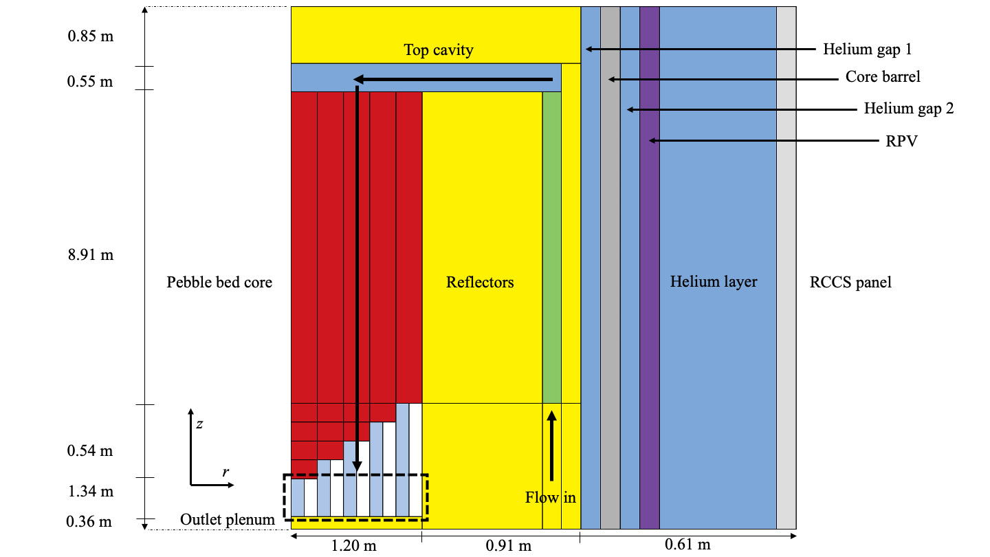
Figure 1: Schematic of the core model of the generic pebble bed reactor.
The SAM model is developed with the so-called core channel approach where the pebble bed is modeled with a number of PbCoreChannel components while the reflectors and other solid structures are modeled with the PbCoupledHeatStructure component. Along with them are the PbOneDFluidCompoenent used for modeling the flow channels. As shown in the above figure, the pebble bed is partitioned into five individual blocks radially where each block is a PbCoreChannel component. In this model, the number of PbCoreChannel components in the radial direction is chosen to match the partitioning of the reactivity feedback coefficients in the work by Stewart et al. (Stewart et al., 2021). Furthermore, the fuel chute is modeled with multiple smaller blocks of PbCoreChannel components to account for its complex geometry. Note that the PbCoreChannel in SAM is essentially a one-dimensional hydraulic component with built-in multi-dimensional heat structures. This allows the specification of hydraulic parameters such as flow area, hydraulic diameter, and surface roughness, as well as solid parameters such as the geometry and material properties of the heat structure. Furthermore, heat transfer parameters such as the heat transfer area density can be provided to the component. Solid, fluid, and heat transfer behaviors are then calculated internally by the PbCoreChannel component according to the provided information. In this model, the PbCoreChannel component is set to have spherical heat structures where the heat-transfer geometry is set as pebble bed.
The solid structures outside of the pebble bed are modeled as concentric rings with the PbCoupledHeatStructure components and are thermally coupled to the adjacent PbOneDFluidComponents when necessary. To ensure proper heat transfer between adjacent solid components, they are thermally coupled in both the radial and axial directions using the SurfaceCoupling component with an arbitrarily large heat transfer coefficient. Furthermore, similar approach is applied to thermally couple adjacent PbCoreChannels to model the core wide radial heat conduction in the pebble bed where the outermost PbCoreChannel is further coupled to the inner surface of the reflector. It is important that the core wide radial heat conduction is modeled correctly as it is one of the primary heat removal mechanisms during loss of forced flow transient scenarios. Heat transfer between solid structures across the helium layers is modeled as radiation heat transfer. Note that the helium layers are assumed as stagnant with no natural convection.
Point kinetics are included in the model for the transient load-following simulation. The point kinetics parameters such as the delayed neutron fractions, the neutron lifetimes, the delayed neutron precursor decay constant, the prompt neutron lifetime, and the reactivity feedback coefficients are obtained from the work by Stewart et al. (Stewart et al., 2021). In this model only temperature reactivity feedback from the fuel, moderator, and reflector regions are considered. Other mechanisms such as coolant reactivity feedback, xenon reactivity feedback, and core expansion reactivity feedback are not considered both in this work and the work by Stewart et al. (Stewart et al., 2021). The distribution of the local reactivity coefficients are illustrated in Figure 2 where the reactivity of the pebble bed is shown to be influenced by the feedback from the fuel, moderator, and reflector. To properly account for the reactivity feedback from different regions, it is necessary to divide the pebble heat structures into three layers of fuel, moderator, and reflector with the correct reactivity coefficients prescribed to each layer. Furthermore, this step is necessary because SAM treats fuel (Doppler) reactivity coefficients differently than moderator/reflector reactivity coefficients. Note that no such distinction is made by SAM between the moderator and reflector reactivity coefficients. This means that in the reflector region where the fuel (Doppler) reactivity coefficients are absent, the local moderator and reflector reactivity coefficients from Stewart et al. (Stewart et al., 2021) can be summed and prescribed directly to the heat structures.
.](../../media/generic-pbr/reactivity-coefficients.png)
Figure 2: Distribution of local reactivity coefficients from Griffin/Pronghorn by Stewart et al. (Stewart et al., 2021).
During steady-state, the one-dimensional fluid components of the model has an inlet velocity 7.17 m/s whose value is determined from the work by Stewart et al. (Stewart et al., 2021) and a pressure outlet boundary condition of 6 MPa. For the solid structures, the top and bottom surfaces are adiabatic while the outer surface of the RCCS panel is given a constant temperature boundary condition of 293.15 K. The total power of the reactor is set at 200 MW. During the transient, the coolant flow rate is reduced to 25% of its nominal value in a span of 900 s, then kept constant at that level for 1800 s, and lastly raised back to the nominal value over 900 s and is held constant to the end of the simulation. Note that other than the coolant flow rate, the other boundary conditions are kept unchanged.
The output files consist of: (1) a csv file that writes all user-specified variables and postprocessors at each time step; (2) a checkpoint folder that saves the snapshots of the simulation data including all meshes, solutions, and stateful object data. They are saved for restarting the run if needed; and (3) an ExodusII file that also has all mesh and solution data. Users can use Paraview to visualize the solution and analyze the data. This tutorial describes the content of the input file, the output files and how the model can be run using the SAM code.
Input Description
SAM uses a block-structured input syntax. Each block begins with square brackets which contain the type of input and ends with empty square brackets. Each block may contain sub-blocks. The blocks in the input file are described in the order as they appear. Before the first block entries, users can define variables and specify their values which are subsequently used in the input model. For example,
emissivity   = 0.8.             # Material emissivity
T_RCCS       = 293.15           # Temperature of RCCS panel
V_in         = 7.186055         # Coolant inlet velocity
In SAM, comments are entered after the # sign
Global parameters
This block contains the parameters such as global initial pressure, velocity, and temperature conditions, the scaling factors for primary variable residuals, etc. For example, to specify global pressure of 6.0e6 Pa, the user can input
global_init_P = 6.0e6
This block also contains a sub-block PBModelParams which specifies the modeling parameters associated with the primitive-variable based fluid model. New users should leave this sub-block unchanged.
EOS
This block specifies the Equation of State. The user can choose from built-in fluid library for common fluids like air, nitrogen, helium, sodium, molten salts, etc. The user can also input the properties of the fluid as constants or function of temperature. For example, the built-in eos for helium can be input as
[EOS]
  [eos]
    type = HeEquationOfState
  []
[]
Functions
Users can define functions for parameters used in the model. These include temporal, spatial, and temperature dependent functions. For example, users can input enthalpy as a function of temperature, power history as a function of time, or power profile as a function of position. Users should be cautious when time-dependent and temperature-dependent functions are in use to avoid confusion between time (t) and temperature (T). Currently, only certain parameters can be made temperature-dependent. These include material properties and the h_gap for the SurfaceCoupling component. The input below specifies the thermal conductivity of fuel pebbles as a function of temperature (in K).
[Functions]
  [k_TRISO]
    # Effective fuel thermal conductivity calculated with Chiew & Glandt model: kp = 4.13 W/(m K)
    type = PiecewiseLinear
    x = '600                700             800             900             1000            1100            1200            1300            1400            1500'
    y = '55.6153061 51.02219975 47.11901811 43.95203134 41.16924224 38.85202882 36.89323509 35.04777834 33.20027175 31.3520767'
  []
[]
MaterialProperties
Material properties are input in this block. The values can be constants or temperature dependent as defined in the Functions block. For example, the properties of fuel pebbles are input as
[MaterialProperties]
  [fuel-mat]
    type = SolidMaterialProps
    k = k_TRISO
    Cp = 1697 # Specific heat
    rho = 1780 # Density assumed the same as normal graphite as suggested by NEA report
  []
[]
The thermal conductivity is defined by the function k_TRISO which appears under the Functions block.
ComponentInputParameters
This block is used to input common features for Components (section below) so that these common features do not need to be repeated in the inputs for Components later on. For example, if pipes are used in various parts of the model and the pipes all have the same diameter, then the diameter can be specified in ComponentsInputParameters and it applies to all pipes used in the model.
[ComponentInputParameters]
  [CoolantChannel]
    type = PBOneDFluidComponentParameters
    eos = eos
    HTC_geometry_type = Pipe
  []
  [Graphite-Fuel]
    type = HeatStructureParameters
    hs_type = cylinder
    dim_hs = 2
    material_hs = 'fuel-mat'
  []
  [Graphite-Reflector]
    type = HeatStructureParameters
    hs_type = cylinder
    dim_hs = 2
    material_hs = 'graphite-mat'
  []
  [SS-Barrel]
    type = HeatStructureParameters
    hs_type = cylinder
    dim_hs = 2
    material_hs = 'ss-mat'
  []
  [SS-RPV]
    type = HeatStructureParameters
    hs_type = cylinder
    dim_hs = 2
    material_hs = 'ss-rpv-mat'
  []
  [Graphite-Reflector-Porous]
    type = HeatStructureParameters
    hs_type = cylinder
    dim_hs = 2
    material_hs = 'graphite-porous-mat'
  []
[]Components
This block provides the specifications for all components that make up the core. The components consist of: reactor, core channels, coolant channels, heat structures (fuel, reflectors, core barrel, RPV and RCCS), junctions for connecting components, and point kinetics. In the reactor component, the reactor power is an input and this includes normal operating power and decay heat. Point kinetics can also be enabled for the core channels through the reactor component.
[Components]
  [reactor]
    type = ReactorPower
    initial_power = 200e6 # Initial total reactor power
    operating_power = 200e6
    pke = 'pke'
    enable_decay_heat = true
    isotope_fission_fraction = '1.0 0.0 0.0 0.0'
  []
[]
Additional point kinetics information is needed by the model and can be provided through the PKE component. Such information includes the delayed neutron fractions, the prompt neutron lifetimes, the delayed neutron precursor decay constant, the names of components with reactivity feedback, and the time for reactivity feedback to start.
[Components]
  [pke]
    type = PointKinetics
    lambda = '1.334e-2 3.273e-2 1.208e-1 3.029e-1 8.501e-1 2.855' # From Griffin/Pronghorn (Table 9 of INL Report [1])
    LAMBDA = 6.519e-4 # From Griffin (Table 9 of INL Report [1])
    betai = '2.344e-4 1.210e-3 1.150e-3 2.588e-3 1.070e-3 4.486e-4' # From Griffin/Pronghorn (Table 9 of INL Report [1])
    feedback_start_time = -200
    feedback_components = 'F-1 F-2 F-3 F-4 F-5 F-6 F-7 F-8 F-9 F-10 F-11 F-12 F-13 F-14 F-15
                               BR-1 BR-2 BR-3 BR-4 BR-5 BR-6 BR-7 BR-8 BR-9 BR-10 BR-11 BR-12 BR-13 BR-14 BR-15 BR-16 BR-17 BR-18 BR-19 BR-20
                               R-4 R-5 R-6 R-7 R-8 R-9 R-10 R-11 R-12 R-13 R-14 R-15 R-16 R-17 R-18 R-19 R-20 R-21 R-22 R-23'
    irk_solver = true # Turn on IRK solver to speed up the simulation for PKE calculation
  []
[]
The coolant channels are modeled as 1-D fluid flow components, and heat structures are modeled as 2-D components. In the bottom reflector region, each coolant channel communicates with its adjacent heat structures through the name_comp_left and name_comp_right variables such as shown below
[Components]
  [BR-6]
    type = PBCoupledHeatStructure
    input_parameters = Graphite-Reflector-Porous
    radius_i = 0.99
    HS_BC_type = 'Coupled Coupled'
    position = '0.0 0 2.065'
    orientation = '0 0 1'
    length = 0.135
    elem_number_axial = 3
    HT_surface_area_density_left = ${aw_BR6_left}
    name_comp_left = CH-5
    HT_surface_area_density_right = ${aw_BR6_right}
    name_comp_right = CH-6
    width_of_hs = '0.1610973'
    elem_number_radial = 5
    moderator_reactivity_feedback = true
    n_layers_moderator = 1
    moderator_reactivity_coefficients = '${moderator_coef_BR6}'
  []
[]
Adjacent heat structures are thermally coupled using SurfaceCoupling to ensure temperature continuity in the radial direction
[Components]
  [coupling_radial_R9_R10]
    type = SurfaceCoupling
    coupling_type = GapHeatTransfer
    h_gap = ${h_gap}
    surface1_name = R-9:outer_wall
    surface2_name = R-10:inner_wall
    radius_1 = 1.72
  []
[]
and axial direction
[Components]
  [coupling_axial_R5_R8]
    type = SurfaceCoupling
    coupling_type = GapHeatTransfer
    h_gap = ${h_gap}
    surface1_name = R-8:top_wall
    surface2_name = R-5:bottom_wall
    radius_1 = 1.9
  []
[]
Note that the coupling in the radial direction is performed on the inner_wall and outer_wall of a heat structure while the coupling in the axial direction is performed on the top_wall and bottom_wall. In both cases the heat transfer coefficient, h_gap, is set to an arbitrarily large value to ensure temperature continuity.
Similarly, SurfaceCoupling is used to thermally couple adjacent core channels to allow for radial heat transfer between the core channels
[Components]
  [coupling_radial_F1_F2]
    type = SurfaceCoupling
    coupling_type = PebbleBedHeatTransfer
    surface1_name = F-1:solid:outer_wall
    surface2_name = F-2:solid:outer_wall
    h_gap = ${h_ZBS_1}
    radius_1 = ${F1_radius}
    radius_2 = ${F2_radius}
    area_ratio = ${F1_F2_ratio}
  []
[]
Note the difference in coupling_type used for the heat structures and the core channels. The former uses GapHeatTransfer and the latter uses PebbleBedHeatTransfer.
In SAM, 1-D fluid components are connected using PBSingleJunction. The following input is used to connect the outlet of component CH-1 to the inlet of component CH-3
[Components]
  [junc_CH1_CH3]
    type = PBSingleJunction
    eos = eos
    inputs = 'CH-1(out)'
    outputs = 'CH-3(in)'
  []
[]
Note that core channels can also be connected with the same approach.
For the components with point kinetics, additional information is required. As mentioned previously, the pebbles in the core channels are divided into three layers of fuel, moderator, and reflector. Using the F-6 core channel block as an example,
    n_heatstruct = 3
    elem_number_of_hs = '5 5 5'
    power_fraction = '${power_fraction_6} 0 0'
    pke_material_type = 'FuelDoppler Moderator Moderator'
    fuel_doppler_coef = ${fuel_coef_F6}
    n_layers_doppler = 1
    n_layers_moderator = 1
    moderator_reactivity_coefficients = '${moderator_coef_F6}; ${reflector_coef_F6}'
the number of layers can be set using the n_heatstruct option. The names, materials, widths, numbers of elements in the radial direction, and power fractions can be provided as a string using the name_of_hs, material_hs, width_of_hs, elem_number_of_hs, and power_fraction options, respectively. Note that because heat is generated only in the fuel region, the power fraction of the this region is set to the desired value with those of the moderator and reflector regions are set to zero. The types of reactivity feedback of each region is specified with the pke_material_type option. The fuel (Doppler) reactivity coefficients are provided with the fuel_doppler_coef option while the moderator/reflector reactivity coefficients are provided with the moderator_reactivity_coefficients option. The numbers of axial elements for point kinetics calculation in the fuel (Doppler) and moderator/reflector regions are provided with the n_layers_doppler and n_layers_moderator options, respectively. Note that the number of PKE axial elements must match the length of the provided reactivity coefficients.
By default, the reactivity feedback in the heat structures of a core channel is calculated using the layered-average solid temperature. However, users can choose to calculate the reactivity feedback in the fuel region with the fuel kernel temperature instead. This can be done by setting
    fuel_kernel_temperature = true
    use_kernel_temperature_doppler = true
Currently, the fuel kernel temperature is calculated using the analytical model implemented in the TINTE code (Gerwin et al., 2010). Additional information is needed as,
    molar_mass_uranium = 0.238
    molar_mass_kernel_material = 0.27
    heavy_metal_loading = 0.009
    local_power_fraction = 1.0
    heat_capacity_kernel_material = 300.0
    modified_heat_flux_resistance = 2.6e-6
  []
[]
Detailed descriptions of these parameters are available in the SAM Theory Manual (Hu et al., 2021) and the TINTE report (Gerwin et al., 2010).
Postprocessors
This block is used to specify the output quantities written to a csv file that can be further processed in Excel or other processing tools such as Python and Matlab. For example, to output the maximum fuel temperature in F-1:
[Postprocessors]
  [max_Tsolid_F1]
    type = NodalExtremeValue
    block = 'F-1:solid:fuel'
    variable = T_solid
  []
[]and the mass flow rate in F-1
[Postprocessors]
  [TotalMassFlowRateInlet_1]
    type = ComponentBoundaryFlow
    input = F-1(in)
  []
[]Preconditioning
This block describes the preconditioner to be used by the preconditioned JFNK solver (available through PETSc). Two options are currently available, the single matrix preconditioner (SMP) and the finite difference preconditioner (FDP). The theory behind the preconditioner can be found in the SAM Theory Manual (Hu et al., 2021). New users can leave this block unchanged.
[Preconditioning]
  [SMP_PJFNK]
    type = SMP
    full = true
    solve_type = 'PJFNK'
    petsc_options_iname = '-pc_type -ksp_gmres_restart'
    petsc_options_value = 'lu 101'
  []
[]Executioner
This block describes the calculation process flow. The user can specify the start time, end time, time step size for the simulation. The user can also choose to use an adaptive time step size with the IterationAdaptiveDT time stepper. Other inputs in this block include PETSc solver options, convergence tolerance, quadrature for elements, etc. which can be left unchanged.
[Executioner]
  type = Transient
  dt = 1
  dtmin = 0.001
  start_time = -172800
  end_time = -210
  dtmax = 10000
  nl_rel_tol = 1e-8
  l_tol = 1e-8
  nl_abs_tol = 1e-8
  nl_max_its = 30
  l_max_its = 200

  # The TimeStepper block can be activated if users
  # wish to enable adaptive time-stepper.
  # [./TimeStepper]
  #     type = IterationAdaptiveDT
  #     growth_factor = 1.25
  #     optimal_iterations = 8
  #     linear_iteration_ratio = 150
  #     dt = 1
  #     cutback_factor = 0.8
  #     cutback_factor_at_failure = 0.8
  # [../]
  [Quadrature]
    type = SIMPSON
    order = SECOND
  []
[]Running the Simulation
SAM can be run on Linux, Unix, and MacOS. Due to its dependence on MOOSE, SAM is not compatible with Windows. SAM can be run from the shell prompt as shown below
sam-opt -i pbr.i
Acknowledgements
This work is supported by U.S. DOE Office of Nuclear Energy’s Nuclear Energy Advanced Modeling and Simulation (NEAMS) program. The submitted manuscript has been created by UChicago Argonne LLC, Operator of Argonne National Laboratory (“Argonne”). Argonne, a U.S. Department of Energy Office of Science laboratory, is operated under Contract No. DE-AC02-06CH11357. The authors would like to acknowledge the support and assistance from Dr. Ryan Stewart and Dr. Paolo Balestra of Idaho National Laboratory in the completion of this work.
References
- H. Gerwin, W. Scherer, A. Lauer, and I. Clifford.
TINTE – Nuclear Calculation Theory Description Report.
Technical Report Jul-4317, Safety Research and Reactor Technology, Institute for Energy Research, 2010.[BibTeX]
@techreport{TINTE2010, author = "Gerwin, H. and Scherer, W. and Lauer, A. and Clifford, I.", number = "Jul-4317", institution = "Safety Research and Reactor Technology, Institute for Energy Research", title = "{TINTE – Nuclear Calculation Theory Description Report}", year = "2010" } - R. Hu, L. Zou, G. Hu, D. Nunez, T. Mui, and T. Fei.
SAM Theory Manual.
Technical Report ANL/NE-17/4 Rev. 1, Argonne National Laboratory, Lemont, IL, 2021.[BibTeX]
@techreport{Hu2021, author = "Hu, R. and Zou, L. and Hu, G. and Nunez, D. and Mui, T. and Fei, T.", address = "Lemont, IL", number = "ANL/NE-17/4 Rev. 1", institution = "Argonne National Laboratory", title = "{SAM Theory Manual}", year = "2021" } - OECDNEA.
PBMR Coupled Neutronics/ Thermal-hydraulics Transient Benchmark the PBMR-400 Core Design.
Technical Report NEA/NSC/DOC(2013)10, Organisation for Economic Co-operation and Development, Nuclear Energy Agency, Paris, France, 2013.[BibTeX]
@techreport{PBMR2013, author = "OECDNEA", address = "Paris, France", number = "NEA/NSC/DOC(2013)10", institution = "Organisation for Economic Co-operation and Development, Nuclear Energy Agency", title = "{PBMR Coupled Neutronics/ Thermal-hydraulics Transient Benchmark the PBMR-400 Core Design}", year = "2013" } - R. Stewart, D. Reger, and P. Balestra.
Demonstrate Capability of NEAMS Tools to Generate Reactor Kinetics Parameters for Pebble-Bed HTGRs Transient Modeling.
Technical Report INL/EXT-21-64176, Idaho National Laboratory, Idaho Falls, ID, 2021.[BibTeX]
@techreport{Stewart2021,
    author = "Stewart, R. and Reger, D. and Balestra, P.",
    address = "Idaho Falls, ID",
    number = "INL/EXT-21-64176",
    institution = "Idaho National Laboratory",
    title = "{Demonstrate Capability of NEAMS Tools to Generate Reactor Kinetics Parameters for Pebble-Bed HTGRs Transient Modeling}",
    year = "2021"
}
(htgr/generic-pbr/pbr.i)
## Author: Zhiee Jhia Ooi, PhD
## Institution: Argonne National Laboratory, 9700 S. Cass Ave, Lemont, IL 60439
################################################################################
## Generic Pebble-Bed HTGR ##
## SAM Single-Application ##
## 1D thermal hydraulics ##
## Primary loop (Core only) ##
################################################################################
# If using or referring to this model, please cite as explained in
# https://mooseframework.inl.gov/virtual_test_bed/citing.html
############################################ Model information ############################################
## 1. This is a SAM model for the generic pebble bed high temperature gas-cooled reactor (HTGR).
## 2. This model only covers the core of the reactor comprising of the pebble bed, the surrounding reflectors,
## core barrel, reactor pressure vessel, and the reactor cavity cooling system (RCCS) panels, as well as the
## upper and lower plena.
## 3. The inlet boundary condition is specified as the helium flow rate while a pressure boundary
## condition is set at the outlet.
## 4. The model is separated into two parts: steady-state and load-following transient. The steady-state simulation
## runs from -172800 s to 0 s, while the transient simulation runs from 0 s to 5000 s.
## 5. Point Kinetics (PKE) are included in the simulation and is activated at t = -210 s. To reduce simulation time, an
## adaptive time step is used during the steady-state non-PKE stage, with a maximum time step size of 10000 s. However,
## to avoid oscillations and instabilities during the PKE stage, the time step must be reduced to no larger than 2 s.
## To do so, the simulation needs to be stopped at -210 s, the maximum time step needs to be changed to 2 s, and then
## the simulation can be recovered.
## 6. Most of the design and operation information of the reactor is obtained from the INL report [1], and is supplemented
## with information from the NEA report [2].
## 7. The PKE parameters such as the reactivity coefficients, the delay neutron precursor fractions, the neutron generation
## time, etc., are obtained from the Griffin/Pronghorn simulation from the INL report [1].
## 8. The pebbles in this model is modeled as a three-layer heat structure comprised of the fuel, moderator, and reflector
## layers. Given that SAM treats Doppler (fuel) and moderator reactivity differently, the distinction is necessary to
## ensure the correct prescription of reactivity coefficients in the pebbles. On the other hand, for the reflector region
## where there is no Doppler reactivity, no distinctions are made between the moderator and reflector reactivities. They
## are summed and prescribed to the reflectors to reduce the complexity of the model.
## Note: The warnings about the dimension of the heat transfer component are expected and do not affect simulation
## results. They will be addressed in upcoming SAM development.
############################################ Main references ############################################
## 1. Stewart, R., Reger, D., and Balestra, P., 'Demonstrate Capability of NEAMS
## Tools to Generate Reactor Kinetics Parameters for Pebble-Bed HTGRs Transient Modeling',
## INL/EXT-21-64176, Idaho National Laboratory, 2021.
##
## 2. 'PBMR Coupled Neutronics/Thermal-hydraulics Transient Benchmark: The PBMR-400 Core Design',
## NEA/NSC/DOC(2013)10, Nuclear Energy Agency - Organisation for Economic Co-operation
## and Development, 2013.
##
## Note: For the remaining of this document, [1] is known as the 'INL report' while [2] is
## known as the 'NEA report'.
########################################################################################################
## If using or referring to this model, please cite as explained in
## https://mooseframework.inl.gov/virtual_test_bed/citing.html
############################################ Miscellaneous properties ############################################
emissivity = 0.8 # According to NEA report [2] graphite and SS are assumed to have a constant emissivity of 0.8
T_RCCS = 293.15 # RCCS outer wall temperature kept at 20 degree C
h_gap = 1e8 # Arbitrarily large value for the gap heat transfer coefficient to mimic solid-solid conduction
V_in = 7.186055 # Calculated based on inlet helium mass flow of 78.6 kg/s (from the INL report) and a flow area
# of 2.04706 m2 at a temperature 533 K and a pressure of 6 MPa
h_ZBS_1 = 43.0158 # Gap heat transfer coefficient for coupling adjacent core channels/flow channels.
h_ZBS_2 = 58.3786 # Calculated with the ZBS correlation at 1000K and 6 MPa for
h_ZBS_3 = 58.3786 # core-wide effective thermal conductivity. The K_eff is then converted to heat transfer coefficient
h_ZBS_4 = 58.3786 # by dividing it by the distance between the centers of adjacent channels.
h_Achenbach = 2068.113361 # Gap heat transfer coefficient for coupling the outermost core channels to the surface of the side reflector.
# Calculated with the Achenbach correlation at 1000K and 6 MPa. The correlation gives thermal conductivity and
# is converted to heat transfer coefficient by dividing it by the distance between the center of the
# outermost core channel to side reflector inner surface of 0.105 m.
############################################ PKE properties ############################################
# PKE properties obtained from the Griffin/Pronghorn simulation presented in the INL report [1].
# Fuel (Doppler) reactivity coefficients (multiplied by the local temperature to fulfill SAM's unit requirement for Doppler reactivity coefficients)
fuel_coef_F1 = -7.62E-03
fuel_coef_F2 = -7.18E-03
fuel_coef_F3 = -7.73E-03
fuel_coef_F4 = -6.79E-03
fuel_coef_F5 = -2.79E-03
fuel_coef_F6 = -2.99E-05
fuel_coef_F7 = -2.81E-05
fuel_coef_F8 = -2.96E-05
fuel_coef_F9 = -2.60E-05
fuel_coef_F10 = -2.28E-05
fuel_coef_F11 = -2.11E-05
fuel_coef_F12 = -2.18E-05
fuel_coef_F13 = -1.20E-05
fuel_coef_F14 = -1.12E-05
fuel_coef_F15 = -1.19E-05
# Moderator reactivity coefficients (NOT multiplied by temperature)
moderator_coef_F6 = -8.12E-09
moderator_coef_F7 = -9.04E-09
moderator_coef_F8 = -1.33E-08
moderator_coef_F9 = -1.59E-08
moderator_coef_F10 = -5.91E-09
moderator_coef_F11 = -7.03E-09
moderator_coef_F12 = -1.19E-08
moderator_coef_F13 = -2.56E-09
moderator_coef_F14 = -4.20E-09
moderator_coef_F15 = -2.75E-09
# Reflector reactivity coefficients (NOT multiplied by temperature)
reflector_coef_F6 = 0.00E+00
reflector_coef_F7 = 5.09E-10
reflector_coef_F8 = 0.00E+00
reflector_coef_F9 = -6.74E-09
reflector_coef_F10 = 0.00E+00
reflector_coef_F11 = 0.00E+00
reflector_coef_F12 = 0.00E+00
reflector_coef_F13 = 0.00E+00
reflector_coef_F14 = -6.03E-10
reflector_coef_F15 = 0.00E+00
# Moderator reactivity coefficients (NOT multiplied by temperature)
moderator_coef_BR1 = -1.35E-08
moderator_coef_BR2 = -2.40E-08
moderator_coef_BR3 = -1.60E-08
moderator_coef_BR4 = -1.24E-08
moderator_coef_BR5 = -1.126101E-08
moderator_coef_BR6 = 7.16974E-09
moderator_coef_BR7 = -1.009311E-08
moderator_coef_BR8 = -1.200361E-08
moderator_coef_BR9 = 4.138E-10
moderator_coef_BR10 = 1.217673E-08
moderator_coef_BR11 = -5.73167E-09
moderator_coef_BR12 = -6.93136E-09
moderator_coef_BR13 = -7.7841E-10
moderator_coef_BR14 = 2.11843E-09
moderator_coef_BR15 = 8.63787E-09
moderator_coef_BR16 = -4.56803E-09
moderator_coef_BR17 = 1.0505E-09
moderator_coef_BR18 = 4.66491E-09
moderator_coef_BR19 = 7.58068E-09
moderator_coef_BR20 = 1.042765E-08
# Reflector reactivity coefficients (NOT multiplied by temperature)
reflector_coef_R6 = 4.35E-08
reflector_coef_R7 = 3.27E-09
reflector_coef_R8 = 0.0
reflector_coef_R9 = 3.12E-08
reflector_coef_R10 = 2.10E-09
reflector_coef_R11 = 0.0
reflector_coef_R12 = 9.38E-09
reflector_coef_R13 = 0.0
reflector_coef_R14 = 0.0
reflector_coef_R15 = 8.63E-09
reflector_coef_R16 = 0.0
reflector_coef_R17 = 0.0
reflector_coef_R18 = 6.84E-09
reflector_coef_R19 = 0.0
reflector_coef_R20 = 0.0
reflector_coef_R21 = 1.003E-08
reflector_coef_R22 = 0.0
reflector_coef_R23 = 0.0
############################################ Thermal hydraulics properties ############################################
# Power fraction of each core channel. Calculated based on the radial power distribution obtained from the INL report [1].
power_fraction_1 = 0.098943344958895
power_fraction_2 = 0.139863269584776
power_fraction_3 = 0.189405592213813
power_fraction_4 = 0.241003959791546
power_fraction_5 = 0.31840010045097
power_fraction_6 = 0.000853753110737
power_fraction_7 = 0.001206839141485
power_fraction_8 = 0.001634325316277
power_fraction_9 = 0.002079552500043
power_fraction_10 = 0.000853753110737
power_fraction_11 = 0.001206839141485
power_fraction_12 = 0.001634325316277
power_fraction_13 = 0.000853753110737
power_fraction_14 = 0.001206839141485
power_fraction_15 = 0.000853753110737
# Number of fuel pebbles of each core channel. Calculated based the volume of each channel and the volume of a fuel pebble (6cm diameter).
n_pebbles_1 = 19610
n_pebbles_2 = 29552
n_pebbles_3 = 42897
n_pebbles_4 = 56243
n_pebbles_5 = 69589
n_pebbles_6 = 296
n_pebbles_7 = 447
n_pebbles_8 = 649
n_pebbles_9 = 850
n_pebbles_10 = 296
n_pebbles_11 = 447
n_pebbles_12 = 649
n_pebbles_13 = 296
n_pebbles_14 = 447
n_pebbles_15 = 296
# Heat transfer area densities of core channels (Units: m2/m3)
# Aw = (Total surface area of pebbles in channel) / (Total volume of fluid in channel)
aw_F1 = 156.41
aw_F2 = 156.41
aw_F3 = 156.41
aw_F4 = 156.41
aw_F5 = 156.41
aw_F6 = 156.41
aw_F7 = 156.41
aw_F8 = 156.41
aw_F9 = 156.41
aw_F10 = 156.41
aw_F11 = 156.41
aw_F12 = 156.41
aw_F13 = 156.41
aw_F14 = 156.41
aw_F15 = 156.41
# Heat transfer area densities of the heat structures in the lower reflector region.
# These are used for the thermal coupling between the heat structures with adjacent
# core channels/heat structures. The 'left' and 'right' notations indicate the left and
# right surfaces of the heat structures.
# Aw = (Surface area of heat structure) / (Fluid volume of adjacent channel)
aw_BR12_left = 22.2222222222222
aw_BR17_left = 22.2222222222222
aw_BR8_left = 23.3486943164363
aw_BR13_left = 23.3486943164363
aw_BR18_left = 23.3486943164363
aw_BR5_left = 22.010582010582
aw_BR9_left = 22.010582010582
aw_BR14_left = 22.010582010582
aw_BR19_left = 22.010582010582
aw_BR3_left = 21.3075060532688
aw_BR6_left = 21.3075060532688
aw_BR10_left = 21.3075060532688
aw_BR15_left = 21.3075060532688
aw_BR20_left = 21.3075060532688
aw_R4_left = 11.8708 # 2*pi*1.2 / (pi*(1.2^2-0.96^2)*0.39)
aw_R6_left = 18.52
aw_R9_left = 18.52
aw_R12_left = 18.52
aw_R15_left = 18.52
aw_R18_left = 18.52
aw_R21_left = 18.52
aw_BR11_right = 19.2450089729875
aw_BR16_right = 19.2450089729875
aw_BR7_right = 21.5229245937167
aw_BR12_right = 21.5229245937167
aw_BR17_right = 21.5229245937167
aw_BR4_right = 20.6888455616507
aw_BR8_right = 20.6888455616507
aw_BR13_right = 20.6888455616507
aw_BR18_right = 20.6888455616507
aw_BR2_right = 20.272255607993
aw_BR5_right = 20.272255607993
aw_BR9_right = 20.272255607993
aw_BR14_right = 20.272255607993
aw_BR19_right = 20.272255607993
aw_BR1_right = 20.023436444044
aw_BR3_right = 20.023436444044
aw_BR6_right = 20.023436444044
aw_BR10_right = 20.023436444044
aw_BR15_right = 20.023436444044
aw_BR20_right = 20.023436444044
# Heat transfer area densities between the upcomer channel
# and the adjacent heat structures.
aw_R4_right = 5.2793124616329
aw_R5_left = 5.83179864947821
# Dimensions of flow channels
A_F1 = 0.158788659083042
A_F6 = 0.158788659083042
A_F10 = 0.158788659083042
A_F13 = 0.158788659083042
A_F15 = 0.158788659083042
A_CH11 = 0.100668573141062
A_CH16 = 0.100668573141062
A_F2 = 0.239285687645974
A_F7 = 0.239285687645974
A_F11 = 0.239285687645974
A_F14 = 0.239285687645974
A_CH7 = 0.153388261311522
A_CH12 = 0.153388261311522
A_CH17 = 0.153388261311522
A_F3 = 0.347350191744155
A_F8 = 0.347350191744155
A_F12 = 0.347350191744155
A_CH4 = 0.222660379323177
A_CH8 = 0.222660379323177
A_CH13 = 0.222660379323177
A_CH18 = 0.222660379323177
A_F4 = 0.455414695842337
A_F9 = 0.455414695842337
A_CH2 = 0.291932497334831
A_CH5 = 0.291932497334831
A_CH9 = 0.291932497334831
A_CH14 = 0.291932497334831
A_CH19 = 0.291932497334831
A_F5 = 0.563479199940519
A_CH1 = 0.361204615346487
A_CH3 = 0.361204615346487
A_CH6 = 0.361204615346487
A_CH10 = 0.361204615346487
A_CH15 = 0.361204615346487
A_CH20 = 0.361204615346487
# Hydraulic diameters of flow channels
Dh_F1 = 0.0383606557377049
Dh_F6 = 0.0383606557377049
Dh_F10 = 0.0383606557377049
Dh_F13 = 0.0383606557377049
Dh_F15 = 0.0383606557377049
Dh_CH11 = 0.0964617092752041
Dh_CH16 = 0.0964617092752041
Dh_F2 = 0.0383606557377049
Dh_F7 = 0.0383606557377049
Dh_F11 = 0.0383606557377049
Dh_F14 = 0.0383606557377049
Dh_CH7 = 0.0891432067117803
Dh_CH12 = 0.0891432067117803
Dh_CH17 = 0.0891432067117803
Dh_F3 = 0.0383606557377049
Dh_F8 = 0.0383606557377049
Dh_F12 = 0.0383606557377049
Dh_CH4 = 0.0936780708180076
Dh_CH8 = 0.0936780708180076
Dh_CH13 = 0.0936780708180076
Dh_CH18 = 0.0936780708180076
Dh_F4 = 0.0383606557377049
Dh_F9 = 0.0383606557377049
Dh_CH2 = 0.0962006476272479
Dh_CH5 = 0.0962006476272479
Dh_CH9 = 0.0962006476272479
Dh_CH14 = 0.0962006476272479
Dh_CH19 = 0.0962006476272479
Dh_F5 = 0.0383606557377049
Dh_CH1 = 0.0978053948460396
Dh_CH3 = 0.0978053948460396
Dh_CH6 = 0.0978053948460396
Dh_CH10 = 0.0978053948460396
Dh_CH15 = 0.0978053948460396
Dh_CH20 = 0.0978053948460396
# Upcomer channel
A_UP1 = 2.04706
Dh_UP1 = 0.36
# Cross sectional area of the upper and lower plena
A_plenum_in = 6.567 # Assume as the cross sectional area between the plenum and the core
A_plenum_out = 7.16 # Cross sectional area of the core
############################################ Surface coupling properties ############################################
# Channel radius
F1_radius = 0.03
F2_radius = 0.03
F3_radius = 0.03
F4_radius = 0.03
F5_radius = 0.03
F6_radius = 0.03
F7_radius = 0.03
F8_radius = 0.03
F9_radius = 0.03
F10_radius = 0.03
F11_radius = 0.03
F12_radius = 0.03
F13_radius = 0.03
F14_radius = 0.03
F15_radius = 0.03
R4_radius = 1.2
# Bottom reflector radius
BR1_radius = 1.15109730257698
BR2_radius = 0.941899676186376
BR4_radius = 0.733160964590996
BR7_radius = 0.52542839664411
# Surface area ratio between the surfaces of two core channels that are thermally coupled together
# Defined as the total surface area of pebbles in the inner core channel to that of the outer core channel
F1_F2_ratio = '${fparse (n_pebbles_1 / n_pebbles_2) }'
F2_F3_ratio = '${fparse (n_pebbles_2 / n_pebbles_3) }'
F3_F4_ratio = '${fparse (n_pebbles_3 / n_pebbles_4) }'
F4_F5_ratio = '${fparse (n_pebbles_4 / n_pebbles_5) }'
F6_F7_ratio = '${fparse (n_pebbles_6 / n_pebbles_7) }'
F7_F8_ratio = '${fparse (n_pebbles_7 / n_pebbles_8) }'
F8_F9_ratio = '${fparse (n_pebbles_8 / n_pebbles_9) }'
F10_F11_ratio = '${fparse (n_pebbles_10 / n_pebbles_11) }'
F11_F12_ratio = '${fparse (n_pebbles_11 / n_pebbles_12) }'
F13_F14_ratio = '${fparse (n_pebbles_13 / n_pebbles_14) }'
# Surface area ration between a core channel and an adjacent heat structure
# Defined as the total surface area of pebbles in the core channel to surface area of the heat structures
F15_BR7_ratio = '${fparse (4.0 * pi * 0.03^2) * n_pebbles_15 / (2 * pi * 0.36 * 0.135)}'
F12_BR2_ratio = '${fparse (4.0 * pi * 0.03^2) * n_pebbles_12 / (2 * pi * 0.78 * 0.135)}'
F9_BR1_ratio = '${fparse (4.0 * pi * 0.03^2) * n_pebbles_9 / (2 * pi * 0.99 * 0.135)}'
F14_BR4_ratio = '${fparse (4.0 * pi * 0.03^2) * n_pebbles_14 / (2 * pi * 0.57 * 0.135)}'
F5_R4_ratio = '${fparse (4.0 * pi * 0.03^2) * n_pebbles_5 / (2 * pi * 1.2 * 8.93)}' # Surface area of pebbles in F-5 divided by surface area of R-4
############################################ Start modeling ############################################
[GlobalParams]
global_init_P = 6e6
global_init_V = ${V_in}
global_init_T = 533
Tsolid_sf = 1e-3
p_order = 2
[]
[Functions]
[time_step]
type = PiecewiseLinear
x = '-172800 -172700 -100 0'
y = '5 300 300 1'
[]
[power_axial_fn]
type = PiecewiseLinear
x = '0 0.5 1 1.5 2 2.5 3 3.5 4 4.5
5 5.5 6 6.5 7 7.5 8 8.5 8.90 8.93'
y = '0.39299934 0.56820578 0.7237816 0.8597268 0.97604136 1.0727253 1.14977861 1.20720129 1.24499334 1.26315477
1.26168557 1.24058574 1.19985528 1.1394942 1.05950249 0.95988015 0.84062718 0.70174359 0.56660312 0.56660312'
axis = x
[]
[power_axial_fn_uniform]
type = PiecewiseLinear
x = '0 0.125 0.135'
y = '1.0 1.0 1.0'
axis = x
[]
[outlet_pressure_fn]
type = PiecewiseLinear
x = '-1.00E+06 0 13 1e6'
y = '6e6 6e6 6e6 6e6'
[]
[V_inlet]
type = PiecewiseLinear
x = '-1.00E+06 0 900 2700 3600 5000'
y = '7.18605 7.18605 1.7965125 1.7965125 7.18605 7.18605'
[]
[rho_func]
type = PiecewiseLinear
y = '0 0'
x = '-1e6 1e6'
[]
# TRISO fuel
[k_TRISO] # Effective fuel thermal conductivity calculated with Chiew & Glandt model: kp = 4.13 W/(m K)
type = PiecewiseLinear
x = '600 700 800 900 1000 1100 1200 1300 1400 1500'
y = '55.6153061 51.02219975 47.11901811 43.95203134 41.16924224 38.85202882 36.89323509 35.04777834 33.20027175 31.3520767'
[]
# Pebble bed effective thermal conductivity calculated from the ZBS correlation
[keff_pebble_bed]
type = PiecewiseLinear
x = '300 400 500 600 700 800 900 1000 1100
1200 1300 1400 1500 1600 1700 1800 1900 2000'
y = '11.940293 12.87749357 14.41727341 16.46031467 18.89508767 21.59454026 24.42480955 27.25852959 29.98755338
32.53156707 34.84117769 36.89601027 38.69951358 40.272406 41.64628551 42.8582912 43.94713743 44.9504677 '
[]
[]
[EOS]
# Built in Helium
[eos]
type = HeEquationOfState
[]
# Built in Air
[air_eos]
type = AirEquationOfState
p_0 = 1.e5
[]
[]
[MaterialProperties]
[ss-mat] # From NEA report [2]
type = SolidMaterialProps
k = 17
Cp = 540
rho = 780
[]
[ss-rpv-mat] # From NEA report [2]
type = SolidMaterialProps
k = 38
Cp = 525
rho = 780
[]
[graphite-mat] # From NEA report [2]
type = SolidMaterialProps
k = 26
Cp = 1697
rho = 1780
[]
[fuel-mat]
type = SolidMaterialProps
k = k_TRISO
Cp = 1697 # Specific heat
rho = 1780 # Density assumed the same as normal graphite as suggested by NEA report
[]
[graphite-porous-mat] # From NEA report [2]: 0.8 of the non-porous graphite properties
type = SolidMaterialProps
k = 20.8
Cp = 1357.6
rho = 1424
[]
[]
[ComponentInputParameters]
[CoolantChannel]
type = PBOneDFluidComponentParameters
eos = eos
HTC_geometry_type = Pipe
[]
[Graphite-Fuel]
type = HeatStructureParameters
hs_type = cylinder
dim_hs = 2
material_hs = 'fuel-mat'
[]
[Graphite-Reflector]
type = HeatStructureParameters
hs_type = cylinder
dim_hs = 2
material_hs = 'graphite-mat'
[]
[SS-Barrel]
type = HeatStructureParameters
hs_type = cylinder
dim_hs = 2
material_hs = 'ss-mat'
[]
[SS-RPV]
type = HeatStructureParameters
hs_type = cylinder
dim_hs = 2
material_hs = 'ss-rpv-mat'
[]
[Graphite-Reflector-Porous]
type = HeatStructureParameters
hs_type = cylinder
dim_hs = 2
material_hs = 'graphite-porous-mat'
[]
[]
[Components]
[pke]
type = PointKinetics
lambda = '1.334e-2 3.273e-2 1.208e-1 3.029e-1 8.501e-1 2.855' # From Griffin/Pronghorn (Table 9 of INL Report [1])
LAMBDA = 6.519e-4 # From Griffin (Table 9 of INL Report [1])
betai = '2.344e-4 1.210e-3 1.150e-3 2.588e-3 1.070e-3 4.486e-4' # From Griffin/Pronghorn (Table 9 of INL Report [1])
feedback_start_time = -200
feedback_components = 'F-1 F-2 F-3 F-4 F-5 F-6 F-7 F-8 F-9 F-10 F-11 F-12 F-13 F-14 F-15
BR-1 BR-2 BR-3 BR-4 BR-5 BR-6 BR-7 BR-8 BR-9 BR-10 BR-11 BR-12 BR-13 BR-14 BR-15 BR-16 BR-17 BR-18 BR-19 BR-20
R-4 R-5 R-6 R-7 R-8 R-9 R-10 R-11 R-12 R-13 R-14 R-15 R-16 R-17 R-18 R-19 R-20 R-21 R-22 R-23'
irk_solver = true # Turn on IRK solver to speed up the simulation for PKE calculation
[]
[reactor]
type = ReactorPower
initial_power = 200e6 # Initial total reactor power
operating_power = 200e6
pke = 'pke'
enable_decay_heat = true
isotope_fission_fraction = '1.0 0.0 0.0 0.0'
[]
[R-1]
type = PBCoupledHeatStructure
input_parameters = Graphite-Reflector
width_of_hs = 1.9
radius_i = 0
HS_BC_type = 'Adiabatic Adiabatic'
position = '0 0 11.95'
orientation = '0 0 1'
length = 0.85
elem_number_radial = 5
elem_number_axial = 3
[]
[F-1]
type = PBCoreChannel
eos = eos
HTC_geometry_type = PebbleBed
d_pebble = 0.06
position = '0 0 11.4'
orientation = '0 0 -1'
roughness = 0.000015
A = ${A_F1}
Dh = ${Dh_F1}
D_heated = ${Dh_F1}
length = 8.93
n_elems = 30
initial_V = ${V_in}
initial_T = 533
Ts_init = 533
initial_P = 6e6
HT_surface_area_density = ${aw_F1}
fuel_type = sphere
power_shape_function = power_axial_fn
dim_hs = 2
porosity = 0.39
HTC_user_option = 'KTA'
material_hs = 'fuel-mat fuel-mat fuel-mat'
name_of_hs = 'fuel moderator reflector'
width_of_hs = '0.025 0.0025 0.0025'
n_heatstruct = 3
elem_number_of_hs = '5 5 5'
power_fraction = '${power_fraction_1} 0 0'
pke_material_type = 'FuelDoppler Moderator Moderator'
fuel_doppler_coef = ${fuel_coef_F1}
n_layers_doppler = 1
n_layers_moderator = 24
moderator_reactivity_coefficients = '-2.41773E-08 -3.98315E-08 -6.02766E-08 -8.7955E-08 -1.26432E-07 -1.70282E-07 -2.25889E-07 -2.8892E-07 -3.64586E-07 -4.40907E-07 -5.04632E-07 -5.18626E-07 -5.07847E-07 -4.70759E-07 -3.42967E-07 -2.29905E-07 -1.28804E-07 -5.85004E-08 -1.8135E-08 0 0 0 0 0 ;
4.91333E-09 9.012E-09 2.00576E-08 2.83693E-08 3.51253E-08 4.57724E-08 5.885E-08 7.0789E-08 7.3222E-08 8.3686E-08 9.3647E-08 9.4312E-08 8.6329E-08 8.5129E-08 9.1274E-08 7.6509E-08 7.1162E-08 5.0449E-08 3.14267E-08 1.09845E-08 5.1141E-10 -1.09373E-08 0 0 '
fuel_kernel_temperature = true
use_kernel_temperature_doppler = true
molar_mass_uranium = 0.238
molar_mass_kernel_material = 0.27
heavy_metal_loading = 0.009
local_power_fraction = 1.0
heat_capacity_kernel_material = 300.0
modified_heat_flux_resistance = 2.6e-6
[]
[F-6]
type = PBCoreChannel
eos = eos
HTC_geometry_type = PebbleBed
d_pebble = 0.06
position = '0 0 2.47'
orientation = '0 0 -1'
roughness = 0.000015
A = ${A_F6}
Dh = ${Dh_F6}
D_heated = ${Dh_F6}
length = 0.135
n_elems = 3
initial_V = ${V_in}
initial_T = 533
Ts_init = 533
initial_P = 6e6
HT_surface_area_density = ${aw_F6}
fuel_type = sphere
power_shape_function = power_axial_fn_uniform
dim_hs = 2
porosity = 0.39
HTC_user_option = 'KTA'
material_hs = 'fuel-mat fuel-mat fuel-mat'
name_of_hs = 'fuel moderator reflector'
width_of_hs = '0.025 0.0025 0.0025'
n_heatstruct = 3
elem_number_of_hs = '5 5 5'
power_fraction = '${power_fraction_6} 0 0'
pke_material_type = 'FuelDoppler Moderator Moderator'
fuel_doppler_coef = ${fuel_coef_F6}
n_layers_doppler = 1
n_layers_moderator = 1
moderator_reactivity_coefficients = '${moderator_coef_F6}; ${reflector_coef_F6}'
fuel_kernel_temperature = true
use_kernel_temperature_doppler = true
molar_mass_uranium = 0.238
molar_mass_kernel_material = 0.27
heavy_metal_loading = 0.009
local_power_fraction = 1.0
heat_capacity_kernel_material = 300.0
modified_heat_flux_resistance = 2.6e-6
[]
[F-10]
type = PBCoreChannel
eos = eos
HTC_geometry_type = PebbleBed
d_pebble = 0.06
position = '0 0 2.335'
orientation = '0 0 -1'
roughness = 0.000015
A = ${A_F10}
Dh = ${Dh_F10}
D_heated = ${Dh_F10}
length = 0.135
n_elems = 3
initial_V = ${V_in}
initial_T = 533
Ts_init = 533
initial_P = 6e6
HT_surface_area_density = ${aw_F10}
fuel_type = sphere
power_shape_function = power_axial_fn_uniform
dim_hs = 2
porosity = 0.39
HTC_user_option = 'KTA'
material_hs = 'fuel-mat fuel-mat fuel-mat'
name_of_hs = 'fuel moderator reflector'
width_of_hs = '0.025 0.0025 0.0025'
n_heatstruct = 3
elem_number_of_hs = '5 5 5'
power_fraction = '${power_fraction_10} 0 0'
pke_material_type = 'FuelDoppler Moderator Moderator'
fuel_doppler_coef = ${fuel_coef_F10}
n_layers_doppler = 1
n_layers_moderator = 1
moderator_reactivity_coefficients = '${moderator_coef_F10}; ${reflector_coef_F10}'
fuel_kernel_temperature = true
use_kernel_temperature_doppler = true
molar_mass_uranium = 0.238
molar_mass_kernel_material = 0.27
heavy_metal_loading = 0.009
local_power_fraction = 1.0
heat_capacity_kernel_material = 300.0
modified_heat_flux_resistance = 2.6e-6
[]
[F-13]
type = PBCoreChannel
eos = eos
HTC_geometry_type = PebbleBed
d_pebble = 0.06
position = '0 0 2.2'
orientation = '0 0 -1'
roughness = 0.000015
A = ${A_F13}
Dh = ${Dh_F13}
D_heated = ${Dh_F13}
length = 0.135
n_elems = 3
initial_V = ${V_in}
initial_T = 533
Ts_init = 533
initial_P = 6e6
HT_surface_area_density = ${aw_F13}
fuel_type = sphere
power_shape_function = power_axial_fn_uniform
dim_hs = 2
porosity = 0.39
HTC_user_option = 'KTA'
material_hs = 'fuel-mat fuel-mat fuel-mat'
name_of_hs = 'fuel moderator reflector'
width_of_hs = '0.025 0.0025 0.0025'
n_heatstruct = 3
elem_number_of_hs = '5 5 5'
power_fraction = '${power_fraction_13} 0 0'
pke_material_type = 'FuelDoppler Moderator Moderator'
fuel_doppler_coef = ${fuel_coef_F13}
n_layers_doppler = 1
n_layers_moderator = 1
moderator_reactivity_coefficients = '${moderator_coef_F13}; ${reflector_coef_F13}'
fuel_kernel_temperature = true
use_kernel_temperature_doppler = true
molar_mass_uranium = 0.238
molar_mass_kernel_material = 0.27
heavy_metal_loading = 0.009
local_power_fraction = 1.0
heat_capacity_kernel_material = 300.0
modified_heat_flux_resistance = 2.6e-6
[]
[F-15]
type = PBCoreChannel
eos = eos
HTC_geometry_type = PebbleBed
d_pebble = 0.06
position = '0 0 2.065'
orientation = '0 0 -1'
roughness = 0.000015
A = ${A_F15}
Dh = ${Dh_F15}
D_heated = ${Dh_F15}
length = 0.135
n_elems = 3
initial_V = ${V_in}
initial_T = 533
Ts_init = 533
initial_P = 6e6
HT_surface_area_density = ${aw_F15}
fuel_type = sphere
power_shape_function = power_axial_fn_uniform
dim_hs = 2
porosity = 0.39
HTC_user_option = 'KTA'
material_hs = 'fuel-mat fuel-mat fuel-mat'
name_of_hs = 'fuel moderator reflector'
width_of_hs = '0.025 0.0025 0.0025'
n_heatstruct = 3
elem_number_of_hs = '5 5 5'
power_fraction = '${power_fraction_15} 0 0'
pke_material_type = 'FuelDoppler Moderator Moderator'
fuel_doppler_coef = ${fuel_coef_F15}
n_layers_doppler = 1
n_layers_moderator = 1
moderator_reactivity_coefficients = '${moderator_coef_F15}; ${reflector_coef_F15}'
fuel_kernel_temperature = true
use_kernel_temperature_doppler = true
molar_mass_uranium = 0.238
molar_mass_kernel_material = 0.27
heavy_metal_loading = 0.009
local_power_fraction = 1.0
heat_capacity_kernel_material = 300.0
modified_heat_flux_resistance = 2.6e-6
[]
[BR-11]
type = PBCoupledHeatStructure
input_parameters = Graphite-Reflector-Porous
radius_i = 0
HS_BC_type = 'Adiabatic Coupled'
position = '0 0 1.54'
orientation = '0 0 1'
length = 0.39
elem_number_axial = 3
HT_surface_area_density_right = ${aw_BR11_right}
name_comp_right = CH-11
width_of_hs = '0.311769'
elem_number_radial = 5
moderator_reactivity_feedback = true
n_layers_moderator = 1
moderator_reactivity_coefficients = '${moderator_coef_BR11}'
[]
[BR-16]
type = PBCoupledHeatStructure
input_parameters = Graphite-Reflector-Porous
radius_i = 0
HS_BC_type = 'Adiabatic Coupled'
position = '0 0 0.59'
orientation = '0 0 1'
length = 0.95
elem_number_axial = 5
HT_surface_area_density_right = ${aw_BR16_right}
name_comp_right = CH-16
width_of_hs = '0.311769'
elem_number_radial = 5
moderator_reactivity_feedback = true
n_layers_moderator = 1
moderator_reactivity_coefficients = '${moderator_coef_BR16}'
[]
[R-24]
type = PBCoupledHeatStructure
input_parameters = Graphite-Reflector
width_of_hs = 0.311769145362398
radius_i = 0
HS_BC_type = 'Adiabatic Adiabatic'
position = '0 0 0.0'
orientation = '0 0 1'
length = 0.59
elem_number_radial = 5
elem_number_axial = 3
[]
[CH-11]
type = PBOneDFluidComponent
input_parameters = CoolantChannel
position = '0.311769145362398 0 1.93'
orientation = '0 0 -1'
length = 0.39
A = ${A_CH11}
Dh = ${Dh_CH11}
HTC_geometry_type = Pipe
n_elems = 3
[]
[CH-16]
type = PBOneDFluidComponent
input_parameters = CoolantChannel
position = '0.311769145362398 0 1.54'
orientation = '0 0 -1'
length = 0.95
A = ${A_CH16}
Dh = ${Dh_CH16}
HTC_geometry_type = Pipe
n_elems = 5
[]
[R-25]
type = PBCoupledHeatStructure
input_parameters = Graphite-Reflector
width_of_hs = 0.048230854637602
radius_i = 0.311769145362398
HS_BC_type = 'Adiabatic Adiabatic'
position = '0.0 0 0.0'
orientation = '0 0 1'
length = 0.59
elem_number_radial = 5
elem_number_axial = 3
[]
[F-2]
type = PBCoreChannel
eos = eos
HTC_geometry_type = PebbleBed
d_pebble = 0.06
position = '0 0.36 11.4'
orientation = '0 0 -1'
roughness = 0.000015
A = ${A_F2}
Dh = ${Dh_F2}
D_heated = ${Dh_F2}
length = 8.93
n_elems = 30
initial_V = ${V_in}
initial_T = 533
Ts_init = 533
initial_P = 6e6
HT_surface_area_density = ${aw_F2}
fuel_type = sphere
power_shape_function = power_axial_fn
dim_hs = 2
porosity = 0.39
HTC_user_option = 'KTA'
material_hs = 'fuel-mat fuel-mat fuel-mat'
name_of_hs = 'fuel moderator reflector'
width_of_hs = '0.025 0.0025 0.0025'
n_heatstruct = 3
elem_number_of_hs = '5 5 5'
power_fraction = '${power_fraction_2} 0 0'
pke_material_type = 'FuelDoppler Moderator Moderator'
fuel_doppler_coef = ${fuel_coef_F2}
n_layers_doppler = 1
n_layers_moderator = 24
moderator_reactivity_coefficients = '-3.1206E-08 -5.0376E-08 -7.3166E-08 -1.04494E-07 -1.42457E-07 -1.89368E-07 -2.4576E-07 -3.11E-07 -3.8324E-07 -4.4223E-07 -4.7318E-07 -4.8782E-07 -4.7237E-07 -4.0142E-07 -2.9106E-07 -1.94784E-07 -1.1736E-07 -5.1004E-08 -1.33765E-08 0 0 0 0 0 ;
6.2158E-09 1.10162E-08 1.54576E-08 2.2245E-08 2.5374E-08 3.2176E-08 5.0429E-08 6.0147E-08 5.3201E-08 5.9858E-08 6.3467E-08 6.5185E-08 8.2931E-08 7.693E-08 7.0086E-08 6.0303E-08 5.3136E-08 3.5494E-08 2.26861E-08 5.8898E-09 -2.8066E-09 -8.7439E-09 0 0 '
fuel_kernel_temperature = true
use_kernel_temperature_doppler = true
molar_mass_uranium = 0.238
molar_mass_kernel_material = 0.27
heavy_metal_loading = 0.009
local_power_fraction = 1.0
heat_capacity_kernel_material = 300.0
modified_heat_flux_resistance = 2.6e-6
[]
[F-7]
type = PBCoreChannel
eos = eos
HTC_geometry_type = PebbleBed
d_pebble = 0.06
position = '0 0.36 2.47'
orientation = '0 0 -1'
roughness = 0.000015
A = ${A_F7}
Dh = ${Dh_F7}
D_heated = ${Dh_F7}
length = 0.135
n_elems = 3
initial_V = ${V_in}
initial_T = 533
Ts_init = 533
initial_P = 6e6
HT_surface_area_density = ${aw_F7}
fuel_type = sphere
power_shape_function = power_axial_fn_uniform
dim_hs = 2
porosity = 0.39
HTC_user_option = 'KTA'
material_hs = 'fuel-mat fuel-mat fuel-mat'
name_of_hs = 'fuel moderator reflector'
width_of_hs = '0.025 0.0025 0.0025'
n_heatstruct = 3
elem_number_of_hs = '5 5 5'
power_fraction = '${power_fraction_7} 0 0'
pke_material_type = 'FuelDoppler Moderator Moderator'
fuel_doppler_coef = ${fuel_coef_F7}
n_layers_doppler = 1
n_layers_moderator = 1
moderator_reactivity_coefficients = '${moderator_coef_F7}; ${reflector_coef_F7}'
fuel_kernel_temperature = true
use_kernel_temperature_doppler = true
molar_mass_uranium = 0.238
molar_mass_kernel_material = 0.27
heavy_metal_loading = 0.009
local_power_fraction = 1.0
heat_capacity_kernel_material = 300.0
modified_heat_flux_resistance = 2.6e-6
[]
[F-11]
type = PBCoreChannel
eos = eos
HTC_geometry_type = PebbleBed
d_pebble = 0.06
position = '0 0.36 2.335'
orientation = '0 0 -1'
roughness = 0.000015
A = ${A_F11}
Dh = ${Dh_F11}
D_heated = ${Dh_F11}
length = 0.135
n_elems = 3
initial_V = ${V_in}
initial_T = 533
Ts_init = 533
initial_P = 6e6
HT_surface_area_density = ${aw_F11}
fuel_type = sphere
power_shape_function = power_axial_fn_uniform
dim_hs = 2
porosity = 0.39
HTC_user_option = 'KTA'
material_hs = 'fuel-mat fuel-mat fuel-mat'
name_of_hs = 'fuel moderator reflector'
width_of_hs = '0.025 0.0025 0.0025'
n_heatstruct = 3
elem_number_of_hs = '5 5 5'
power_fraction = '${power_fraction_11} 0 0'
pke_material_type = 'FuelDoppler Moderator Moderator'
fuel_doppler_coef = ${fuel_coef_F11}
n_layers_doppler = 1
n_layers_moderator = 1
moderator_reactivity_coefficients = '${moderator_coef_F11}; ${reflector_coef_F11}'
fuel_kernel_temperature = true
use_kernel_temperature_doppler = true
molar_mass_uranium = 0.238
molar_mass_kernel_material = 0.27
heavy_metal_loading = 0.009
local_power_fraction = 1.0
heat_capacity_kernel_material = 300.0
modified_heat_flux_resistance = 2.6e-6
[]
[F-14]
type = PBCoreChannel
eos = eos
HTC_geometry_type = PebbleBed
d_pebble = 0.06
position = '0 0.36 2.2'
orientation = '0 0 -1'
roughness = 0.000015
A = ${A_F14}
Dh = ${Dh_F14}
D_heated = ${Dh_F14}
length = 0.135
n_elems = 3
initial_V = ${V_in}
initial_T = 533
Ts_init = 533
initial_P = 6e6
HT_surface_area_density = ${aw_F14}
fuel_type = sphere
power_shape_function = power_axial_fn_uniform
dim_hs = 2
porosity = 0.39
HTC_user_option = 'KTA'
material_hs = 'fuel-mat fuel-mat fuel-mat'
name_of_hs = 'fuel moderator reflector'
width_of_hs = '0.025 0.0025 0.0025'
n_heatstruct = 3
elem_number_of_hs = '5 5 5'
power_fraction = '${power_fraction_14} 0 0'
pke_material_type = 'FuelDoppler Moderator Moderator'
fuel_doppler_coef = ${fuel_coef_F14}
n_layers_doppler = 1
n_layers_moderator = 1
moderator_reactivity_coefficients = '${moderator_coef_F14}; ${reflector_coef_F14}'
fuel_kernel_temperature = true
use_kernel_temperature_doppler = true
molar_mass_uranium = 0.238
molar_mass_kernel_material = 0.27
heavy_metal_loading = 0.009
local_power_fraction = 1.0
heat_capacity_kernel_material = 300.0
modified_heat_flux_resistance = 2.6e-6
[]
[BR-7]
type = PBCoupledHeatStructure
input_parameters = Graphite-Reflector-Porous
radius_i = 0.36
HS_BC_type = 'Adiabatic Coupled'
position = '0.0 0 1.93'
orientation = '0 0 1'
length = 0.135
elem_number_axial = 3
HT_surface_area_density_right = ${aw_BR7_right}
name_comp_right = CH-7
width_of_hs = '0.165428'
elem_number_radial = 5
moderator_reactivity_feedback = true
n_layers_moderator = 1
moderator_reactivity_coefficients = '${moderator_coef_BR7}'
[]
[BR-12]
type = PBCoupledHeatStructure
input_parameters = Graphite-Reflector-Porous
radius_i = 0.36
HS_BC_type = 'Coupled Coupled'
position = '0.0 0 1.54'
orientation = '0 0 1'
length = 0.39
elem_number_axial = 3
HT_surface_area_density_left = ${aw_BR12_left}
name_comp_left = CH-11
HT_surface_area_density_right = ${aw_BR12_right}
name_comp_right = CH-12
width_of_hs = '0.165428'
elem_number_radial = 5
moderator_reactivity_feedback = true
n_layers_moderator = 1
moderator_reactivity_coefficients = '${moderator_coef_BR12}'
[]
[BR-17]
type = PBCoupledHeatStructure
input_parameters = Graphite-Reflector-Porous
radius_i = 0.36
HS_BC_type = 'Coupled Coupled'
position = '0.0 0 0.59'
orientation = '0 0 1'
length = 0.95
elem_number_axial = 5
HT_surface_area_density_left = ${aw_BR17_left}
name_comp_left = CH-16
HT_surface_area_density_right = ${aw_BR17_right}
name_comp_right = CH-17
width_of_hs = '0.165428'
elem_number_radial = 5
moderator_reactivity_feedback = true
n_layers_moderator = 1
moderator_reactivity_coefficients = '${moderator_coef_BR17}'
[]
[R-26]
type = PBCoupledHeatStructure
input_parameters = Graphite-Reflector
width_of_hs = 0.16542839664411
radius_i = 0.36
HS_BC_type = 'Adiabatic Adiabatic'
position = '0.0 0 0.0'
orientation = '0 0 1'
length = 0.59
elem_number_radial = 5
elem_number_axial = 3
[]
[CH-7]
type = PBOneDFluidComponent
input_parameters = CoolantChannel
position = '0.52542839664411 0 2.065'
orientation = '0 0 -1'
length = 0.135
A = ${A_CH7}
Dh = ${Dh_CH7}
HTC_geometry_type = Pipe
n_elems = 3
[]
[CH-12]
type = PBOneDFluidComponent
input_parameters = CoolantChannel
position = '0.52542839664411 0 1.93'
orientation = '0 0 -1'
length = 0.39
A = ${A_CH12}
Dh = ${Dh_CH12}
HTC_geometry_type = Pipe
n_elems = 3
[]
[CH-17]
type = PBOneDFluidComponent
input_parameters = CoolantChannel
position = '0.52542839664411 0 1.54'
orientation = '0 0 -1'
length = 0.95
A = ${A_CH17}
Dh = ${Dh_CH17}
HTC_geometry_type = Pipe
n_elems = 5
[]
[R-27]
type = PBCoupledHeatStructure
input_parameters = Graphite-Reflector
width_of_hs = 0.04457160335589
radius_i = 0.52542839664411
HS_BC_type = 'Adiabatic Adiabatic'
position = '0.0 0 0.0'
orientation = '0 0 1'
length = 0.59
elem_number_radial = 5
elem_number_axial = 3
[]
[F-3]
type = PBCoreChannel
eos = eos
HTC_geometry_type = PebbleBed
d_pebble = 0.06
position = '0 0.57 11.4'
orientation = '0 0 -1'
roughness = 0.000015
A = ${A_F3}
Dh = ${Dh_F3}
D_heated = ${Dh_F3}
length = 8.93
n_elems = 30
initial_V = ${V_in}
initial_T = 533
Ts_init = 533
initial_P = 6e6
HT_surface_area_density = ${aw_F3}
fuel_type = sphere
power_shape_function = power_axial_fn
dim_hs = 2
porosity = 0.39
HTC_user_option = 'KTA'
material_hs = 'fuel-mat fuel-mat fuel-mat'
name_of_hs = 'fuel moderator reflector'
width_of_hs = '0.025 0.0025 0.0025'
n_heatstruct = 3
elem_number_of_hs = '5 5 5'
power_fraction = '${power_fraction_3} 0 0'
pke_material_type = 'FuelDoppler Moderator Moderator'
fuel_doppler_coef = ${fuel_coef_F3}
n_layers_doppler = 1
n_layers_moderator = 24
moderator_reactivity_coefficients = '-4.1502E-08 -6.6531E-08 -9.7965E-08 -1.39468E-07 -1.87341E-07 -2.4789E-07 -3.2676E-07 -4.0955E-07 -4.8555E-07 -5.2862E-07 -5.7208E-07 -5.9023E-07 -5.5259E-07 -4.4628E-07 -3.2909E-07 -2.1846E-07 -1.24808E-07 -5.1652E-08 -9.5243E-09 0 0 0 0 0 ;
4.8208E-09 9.0552E-09 1.28369E-08 1.84375E-08 2.4855E-08 3.1243E-08 4.5786E-08 5.4986E-08 4.2126E-08 4.5781E-08 6.3294E-08 6.4477E-08 6.8275E-08 6.6649E-08 5.6315E-08 4.8701E-08 5.1472E-08 3.6056E-08 1.83018E-08 6.9841E-10 -4.7966E-09 -8.0451E-09 0 0 '
fuel_kernel_temperature = true
use_kernel_temperature_doppler = true
molar_mass_uranium = 0.238
molar_mass_kernel_material = 0.27
heavy_metal_loading = 0.009
local_power_fraction = 1.0
heat_capacity_kernel_material = 300.0
modified_heat_flux_resistance = 2.6e-6
[]
[F-8]
type = PBCoreChannel
eos = eos
HTC_geometry_type = PebbleBed
d_pebble = 0.06
position = '0 0.57 2.47'
orientation = '0 0 -1'
roughness = 0.000015
A = ${A_F8}
Dh = ${Dh_F8}
D_heated = ${Dh_F8}
length = 0.135
n_elems = 3
initial_V = ${V_in}
initial_T = 533
Ts_init = 533
initial_P = 6e6
HT_surface_area_density = ${aw_F8}
fuel_type = sphere
power_shape_function = power_axial_fn_uniform
dim_hs = 2
porosity = 0.39
HTC_user_option = 'KTA'
material_hs = 'fuel-mat fuel-mat fuel-mat'
name_of_hs = 'fuel moderator reflector'
width_of_hs = '0.025 0.0025 0.0025'
n_heatstruct = 3
elem_number_of_hs = '5 5 5'
power_fraction = '${power_fraction_8} 0 0'
pke_material_type = 'FuelDoppler Moderator Moderator'
fuel_doppler_coef = ${fuel_coef_F8}
n_layers_doppler = 1
n_layers_moderator = 1
moderator_reactivity_coefficients = '${moderator_coef_F8}; ${reflector_coef_F8}'
fuel_kernel_temperature = true
use_kernel_temperature_doppler = true
molar_mass_uranium = 0.238
molar_mass_kernel_material = 0.27
heavy_metal_loading = 0.009
local_power_fraction = 1.0
heat_capacity_kernel_material = 300.0
modified_heat_flux_resistance = 2.6e-6
[]
[F-12]
type = PBCoreChannel
eos = eos
HTC_geometry_type = PebbleBed
d_pebble = 0.06
position = '0 0.57 2.335'
orientation = '0 0 -1'
roughness = 0.000015
A = ${A_F12}
Dh = ${Dh_F12}
D_heated = ${Dh_F12}
length = 0.135
n_elems = 3
initial_V = ${V_in}
initial_T = 533
Ts_init = 533
initial_P = 6e6
HT_surface_area_density = ${aw_F12}
fuel_type = sphere
power_shape_function = power_axial_fn_uniform
dim_hs = 2
porosity = 0.39
HTC_user_option = 'KTA'
material_hs = 'fuel-mat fuel-mat fuel-mat'
name_of_hs = 'fuel moderator reflector'
width_of_hs = '0.025 0.0025 0.0025'
n_heatstruct = 3
elem_number_of_hs = '5 5 5'
power_fraction = '${power_fraction_12} 0 0'
pke_material_type = 'FuelDoppler Moderator Moderator'
fuel_doppler_coef = ${fuel_coef_F12}
n_layers_doppler = 1
n_layers_moderator = 1
moderator_reactivity_coefficients = '${moderator_coef_F12}; ${reflector_coef_F12}'
fuel_kernel_temperature = true
use_kernel_temperature_doppler = true
molar_mass_uranium = 0.238
molar_mass_kernel_material = 0.27
heavy_metal_loading = 0.009
local_power_fraction = 1.0
heat_capacity_kernel_material = 300.0
modified_heat_flux_resistance = 2.6e-6
[]
[BR-4]
type = PBCoupledHeatStructure
input_parameters = Graphite-Reflector-Porous
radius_i = 0.57
HS_BC_type = 'Adiabatic Coupled'
position = '0.0 0 2.065'
orientation = '0 0 1'
length = 0.135
elem_number_axial = 3
HT_surface_area_density_right = ${aw_BR4_right}
name_comp_right = CH-4
width_of_hs = '0.16316'
elem_number_radial = 5
moderator_reactivity_feedback = true
n_layers_moderator = 1
moderator_reactivity_coefficients = '${moderator_coef_BR4}'
[]
[BR-8]
type = PBCoupledHeatStructure
input_parameters = Graphite-Reflector-Porous
radius_i = 0.57
HS_BC_type = 'Coupled Coupled'
position = '0.0 0 1.93'
orientation = '0 0 1'
length = 0.135
elem_number_axial = 3
HT_surface_area_density_left = ${aw_BR8_left}
name_comp_left = CH-7
HT_surface_area_density_right = ${aw_BR8_right}
name_comp_right = CH-8
width_of_hs = '0.16316'
elem_number_radial = 5
moderator_reactivity_feedback = true
n_layers_moderator = 1
moderator_reactivity_coefficients = '${moderator_coef_BR8}'
[]
[BR-13]
type = PBCoupledHeatStructure
input_parameters = Graphite-Reflector-Porous
radius_i = 0.57
HS_BC_type = 'Coupled Coupled'
position = '0.0 0 1.54'
orientation = '0 0 1'
length = 0.39
elem_number_axial = 3
HT_surface_area_density_left = ${aw_BR13_left}
name_comp_left = CH-12
HT_surface_area_density_right = ${aw_BR13_right}
name_comp_right = CH-13
width_of_hs = '0.16316'
elem_number_radial = 5
moderator_reactivity_feedback = true
n_layers_moderator = 1
moderator_reactivity_coefficients = '${moderator_coef_BR13}'
[]
[BR-18]
type = PBCoupledHeatStructure
input_parameters = Graphite-Reflector-Porous
radius_i = 0.57
HS_BC_type = 'Coupled Coupled'
position = '0.0 0 0.59'
orientation = '0 0 1'
length = 0.95
elem_number_axial = 5
HT_surface_area_density_left = ${aw_BR18_left}
name_comp_left = CH-17
HT_surface_area_density_right = ${aw_BR18_right}
name_comp_right = CH-18
width_of_hs = '0.16316'
elem_number_radial = 5
moderator_reactivity_feedback = true
n_layers_moderator = 1
moderator_reactivity_coefficients = '${moderator_coef_BR18}'
[]
[R-28]
type = PBCoupledHeatStructure
input_parameters = Graphite-Reflector
width_of_hs = 0.163160964590996
radius_i = 0.57
HS_BC_type = 'Adiabatic Adiabatic'
position = '0.0 0 0.0'
orientation = '0 0 1'
length = 0.59
elem_number_radial = 5
elem_number_axial = 3
[]
[CH-4]
type = PBOneDFluidComponent
input_parameters = CoolantChannel
position = '0.733160964590996 0 2.2'
orientation = '0 0 -1'
length = 0.135
A = ${A_CH4}
Dh = ${Dh_CH4}
HTC_geometry_type = Pipe
n_elems = 3
[]
[CH-8]
type = PBOneDFluidComponent
input_parameters = CoolantChannel
position = '0.733160964590996 0 2.065'
orientation = '0 0 -1'
length = 0.135
A = ${A_CH8}
Dh = ${Dh_CH8}
HTC_geometry_type = Pipe
n_elems = 3
[]
[CH-13]
type = PBOneDFluidComponent
input_parameters = CoolantChannel
position = '0.733160964590996 0 1.93'
orientation = '0 0 -1'
length = 0.39
A = ${A_CH13}
Dh = ${Dh_CH13}
HTC_geometry_type = Pipe
n_elems = 3
[]
[CH-18]
type = PBOneDFluidComponent
input_parameters = CoolantChannel
position = '0.733160964590996 0 1.54'
orientation = '0 0 -1'
length = 0.95
A = ${A_CH18}
Dh = ${Dh_CH18}
HTC_geometry_type = Pipe
n_elems = 5
[]
[R-29]
type = PBCoupledHeatStructure
input_parameters = Graphite-Reflector
width_of_hs = 0.046839035409004
radius_i = 0.733160964590996
HS_BC_type = 'Adiabatic Adiabatic'
position = '0.0 0 0.0'
orientation = '0 0 1'
length = 0.59
elem_number_radial = 5
elem_number_axial = 3
[]
[F-4]
type = PBCoreChannel
eos = eos
HTC_geometry_type = PebbleBed
d_pebble = 0.06
position = '0 0.78 11.4'
orientation = '0 0 -1'
roughness = 0.000015
A = ${A_F4}
Dh = ${Dh_F4}
D_heated = ${Dh_F4}
length = 8.93
n_elems = 30
initial_V = ${V_in}
initial_T = 533
Ts_init = 533
initial_P = 6e6
HT_surface_area_density = ${aw_F4}
fuel_type = sphere
power_shape_function = power_axial_fn
dim_hs = 2
porosity = 0.39
HTC_user_option = 'KTA'
material_hs = 'fuel-mat fuel-mat fuel-mat'
name_of_hs = 'fuel moderator reflector'
width_of_hs = '0.025 0.0025 0.0025'
n_heatstruct = 3
elem_number_of_hs = '5 5 5'
power_fraction = '${power_fraction_4} 0 0'
pke_material_type = 'FuelDoppler Moderator Moderator'
fuel_doppler_coef = ${fuel_coef_F4}
n_layers_doppler = 1
n_layers_moderator = 24
moderator_reactivity_coefficients = '-5.1478E-08 -8.238E-08 -1.23281E-07 -1.75574E-07 -2.3964E-07 -3.1655E-07 -4.1231E-07 -5.1694E-07 -6.2474E-07 -6.9342E-07 -7.372E-07 -7.6304E-07 -7.5774E-07 -6.1366E-07 -4.4703E-07 -2.9582E-07 -1.6193E-07 -6.6565E-08 -1.24153E-08 0 0 0 0 0 ;
-1.14807E-08 -1.60696E-08 -2.26269E-08 -2.89545E-08 -2.9162E-08 -3.4328E-08 -4.5102E-08 -4.9339E-08 -5.7451E-08 -6.4695E-08 -5.8815E-08 -6.7572E-08 -7.8757E-08 -7.9902E-08 -8.3934E-08 -7.8444E-08 -6.5091E-08 -5.1167E-08 -3.72781E-08 -2.9257E-08 -1.33766E-08 -7.4375E-09 0 0 '
fuel_kernel_temperature = true
use_kernel_temperature_doppler = true
molar_mass_uranium = 0.238
molar_mass_kernel_material = 0.27
heavy_metal_loading = 0.009
local_power_fraction = 1.0
heat_capacity_kernel_material = 300.0
modified_heat_flux_resistance = 2.6e-6
[]
[F-9]
type = PBCoreChannel
eos = eos
HTC_geometry_type = PebbleBed
d_pebble = 0.06
position = '0 0.78 2.47'
orientation = '0 0 -1'
roughness = 0.000015
A = ${A_F9}
Dh = ${Dh_F9}
D_heated = ${Dh_F9}
length = 0.135
n_elems = 3
initial_V = ${V_in}
initial_T = 533
Ts_init = 533
initial_P = 6e6
HT_surface_area_density = ${aw_F9}
fuel_type = sphere
power_shape_function = power_axial_fn_uniform
dim_hs = 2
porosity = 0.39
HTC_user_option = 'KTA'
material_hs = 'fuel-mat fuel-mat fuel-mat'
name_of_hs = 'fuel moderator reflector'
width_of_hs = '0.025 0.0025 0.0025'
n_heatstruct = 3
elem_number_of_hs = '5 5 5'
power_fraction = '${power_fraction_9} 0 0'
pke_material_type = 'FuelDoppler Moderator Moderator'
fuel_doppler_coef = ${fuel_coef_F9}
n_layers_doppler = 1
n_layers_moderator = 1
moderator_reactivity_coefficients = '${moderator_coef_F9}; ${reflector_coef_F9}'
fuel_kernel_temperature = true
use_kernel_temperature_doppler = true
molar_mass_uranium = 0.238
molar_mass_kernel_material = 0.27
heavy_metal_loading = 0.009
local_power_fraction = 1.0
heat_capacity_kernel_material = 300.0
modified_heat_flux_resistance = 2.6e-6
[]
[BR-2]
type = PBCoupledHeatStructure
input_parameters = Graphite-Reflector-Porous
radius_i = 0.78
HS_BC_type = 'Adiabatic Coupled'
position = '0.0 0 2.2'
orientation = '0 0 1'
length = 0.135
elem_number_axial = 3
HT_surface_area_density_right = ${aw_BR2_right}
name_comp_right = CH-2
width_of_hs = '0.1618996'
elem_number_radial = 5
moderator_reactivity_feedback = true
n_layers_moderator = 1
moderator_reactivity_coefficients = '${moderator_coef_BR2}'
[]
[BR-5]
type = PBCoupledHeatStructure
input_parameters = Graphite-Reflector-Porous
radius_i = 0.78
HS_BC_type = 'Coupled Coupled'
position = '0.0 0 2.065'
orientation = '0 0 1'
length = 0.135
elem_number_axial = 3
HT_surface_area_density_left = ${aw_BR5_left}
name_comp_left = CH-4
HT_surface_area_density_right = ${aw_BR5_right}
name_comp_right = CH-5
width_of_hs = '0.1618996'
elem_number_radial = 5
moderator_reactivity_feedback = true
n_layers_moderator = 1
moderator_reactivity_coefficients = '${moderator_coef_BR5}'
[]
[BR-9]
type = PBCoupledHeatStructure
input_parameters = Graphite-Reflector-Porous
radius_i = 0.78
HS_BC_type = 'Coupled Coupled'
position = '0.0 0 1.93'
orientation = '0 0 1'
length = 0.135
elem_number_axial = 3
HT_surface_area_density_left = ${aw_BR9_left}
name_comp_left = CH-8
HT_surface_area_density_right = ${aw_BR9_right}
name_comp_right = CH-9
width_of_hs = '0.1618996'
elem_number_radial = 5
moderator_reactivity_feedback = true
n_layers_moderator = 1
moderator_reactivity_coefficients = '${moderator_coef_BR9}'
[]
[BR-14]
type = PBCoupledHeatStructure
input_parameters = Graphite-Reflector-Porous
radius_i = 0.78
HS_BC_type = 'Coupled Coupled'
position = '0.0 0 1.54'
orientation = '0 0 1'
length = 0.39
elem_number_axial = 3
HT_surface_area_density_left = ${aw_BR14_left}
name_comp_left = CH-13
HT_surface_area_density_right = ${aw_BR14_right}
name_comp_right = CH-14
width_of_hs = '0.1618996'
elem_number_radial = 5
moderator_reactivity_feedback = true
n_layers_moderator = 1
moderator_reactivity_coefficients = '${moderator_coef_BR14}'
[]
[BR-19]
type = PBCoupledHeatStructure
input_parameters = Graphite-Reflector-Porous
radius_i = 0.78
HS_BC_type = 'Coupled Coupled'
position = '0.0 0 0.59'
orientation = '0 0 1'
length = 0.95
elem_number_axial = 5
HT_surface_area_density_left = ${aw_BR19_left}
name_comp_left = CH-18
HT_surface_area_density_right = ${aw_BR19_right}
name_comp_right = CH-19
width_of_hs = '0.1618996'
elem_number_radial = 5
moderator_reactivity_feedback = true
n_layers_moderator = 1
moderator_reactivity_coefficients = '${moderator_coef_BR19}'
[]
[R-30]
type = PBCoupledHeatStructure
input_parameters = Graphite-Reflector
width_of_hs = 0.161899676186376
radius_i = 0.78
HS_BC_type = 'Adiabatic Adiabatic'
position = '0.0 0 0.0'
orientation = '0 0 1'
length = 0.59
elem_number_radial = 5
elem_number_axial = 3
[]
[CH-2]
type = PBOneDFluidComponent
input_parameters = CoolantChannel
position = '0.941899676186376 0 2.335'
orientation = '0 0 -1'
length = 0.135
A = ${A_CH2}
Dh = ${Dh_CH2}
HTC_geometry_type = Pipe
n_elems = 3
[]
[CH-5]
type = PBOneDFluidComponent
input_parameters = CoolantChannel
position = '0.941899676186376 0 2.2'
orientation = '0 0 -1'
length = 0.135
A = ${A_CH5}
Dh = ${Dh_CH5}
HTC_geometry_type = Pipe
n_elems = 3
[]
[CH-9]
type = PBOneDFluidComponent
input_parameters = CoolantChannel
position = '0.941899676186376 0 2.065'
orientation = '0 0 -1'
length = 0.135
A = ${A_CH9}
Dh = ${Dh_CH9}
HTC_geometry_type = Pipe
n_elems = 3
[]
[CH-14]
type = PBOneDFluidComponent
input_parameters = CoolantChannel
position = '0.941899676186376 0 1.93'
orientation = '0 0 -1'
length = 0.39
A = ${A_CH14}
Dh = ${Dh_CH14}
HTC_geometry_type = Pipe
n_elems = 3
[]
[CH-19]
type = PBOneDFluidComponent
input_parameters = CoolantChannel
position = '0.941899676186376 0 1.54'
orientation = '0 0 -1'
length = 0.95
A = ${A_CH19}
Dh = ${Dh_CH19}
HTC_geometry_type = Pipe
n_elems = 5
[]
[R-31]
type = PBCoupledHeatStructure
input_parameters = Graphite-Reflector
width_of_hs = 0.048100323813624
radius_i = 0.941899676186376
HS_BC_type = 'Adiabatic Adiabatic'
position = '0.0 0 0.0'
orientation = '0 0 1'
length = 0.59
elem_number_radial = 5
elem_number_axial = 3
[]
[F-5]
type = PBCoreChannel
eos = eos
HTC_geometry_type = PebbleBed
d_pebble = 0.06
position = '0 0.99 11.4'
orientation = '0 0 -1'
roughness = 0.000015
A = ${A_F5}
Dh = ${Dh_F5}
D_heated = ${Dh_F5}
length = 8.93
n_elems = 30
initial_V = ${V_in}
initial_T = 533
Ts_init = 533
initial_P = 6e6
HT_surface_area_density = ${aw_F5}
fuel_type = sphere
power_shape_function = power_axial_fn
dim_hs = 2
porosity = 0.39
HTC_user_option = 'KTA'
material_hs = 'fuel-mat fuel-mat fuel-mat'
name_of_hs = 'fuel moderator reflector'
width_of_hs = '0.025 0.0025 0.0025'
n_heatstruct = 3
elem_number_of_hs = '5 5 5'
power_fraction = '${power_fraction_5} 0 0'
pke_material_type = 'FuelDoppler Moderator Moderator'
fuel_doppler_coef = ${fuel_coef_F5}
n_layers_doppler = 1
n_layers_moderator = 24
moderator_reactivity_coefficients = '-3.70306E-08 -5.94132E-08 -8.9707E-08 -1.28418E-07 -1.78363E-07 -2.38849E-07 -3.14346E-07 -4.02238E-07 -5.03327E-07 -6.07354E-07 -6.28733E-07 -6.58135E-07 -6.83367E-07 -6.0209E-07 -4.524085E-07 -3.048042E-07 -1.62664E-07 -6.80384E-08 -7.361E-09 7.8554E-09 8.6996E-09 2.4915E-09 0 0 ;
7.29199999999999E-09 2.2746E-08 3.8951E-08 8.2539E-08 1.28962E-07 2.19077E-07 2.5175E-07 2.9007E-07 3.2917E-07 3.6051E-07 4.0184E-07 4.7956E-07 4.9371E-07 5.601E-07 5.6805E-07 5.4002E-07 4.5629E-07 3.696E-07 2.3873E-07 9.5877E-08 6.68E-09 4.29100000000001E-10 1.75E-09 9.532E-10 '
fuel_kernel_temperature = true
use_kernel_temperature_doppler = true
molar_mass_uranium = 0.238
molar_mass_kernel_material = 0.27
heavy_metal_loading = 0.009
local_power_fraction = 1.0
heat_capacity_kernel_material = 300.0
modified_heat_flux_resistance = 2.6e-6
[]
[BR-1]
type = PBCoupledHeatStructure
input_parameters = Graphite-Reflector-Porous
radius_i = 0.99
HS_BC_type = 'Adiabatic Coupled'
position = '0.0 0 2.335'
orientation = '0 0 1'
length = 0.135
elem_number_axial = 3
HT_surface_area_density_right = ${aw_BR1_right}
name_comp_right = CH-1
width_of_hs = '0.1610973'
elem_number_radial = 5
moderator_reactivity_feedback = true
n_layers_moderator = 1
moderator_reactivity_coefficients = '${moderator_coef_BR1}'
[]
[BR-3]
type = PBCoupledHeatStructure
input_parameters = Graphite-Reflector-Porous
radius_i = 0.99
HS_BC_type = 'Coupled Coupled'
position = '0.0 0 2.2'
orientation = '0 0 1'
length = 0.135
elem_number_axial = 3
HT_surface_area_density_left = ${aw_BR3_left}
name_comp_left = CH-2
HT_surface_area_density_right = ${aw_BR3_right}
name_comp_right = CH-3
width_of_hs = '0.1610973'
elem_number_radial = 5
moderator_reactivity_feedback = true
n_layers_moderator = 1
moderator_reactivity_coefficients = '${moderator_coef_BR3}'
[]
[BR-6]
type = PBCoupledHeatStructure
input_parameters = Graphite-Reflector-Porous
radius_i = 0.99
HS_BC_type = 'Coupled Coupled'
position = '0.0 0 2.065'
orientation = '0 0 1'
length = 0.135
elem_number_axial = 3
HT_surface_area_density_left = ${aw_BR6_left}
name_comp_left = CH-5
HT_surface_area_density_right = ${aw_BR6_right}
name_comp_right = CH-6
width_of_hs = '0.1610973'
elem_number_radial = 5
moderator_reactivity_feedback = true
n_layers_moderator = 1
moderator_reactivity_coefficients = '${moderator_coef_BR6}'
[]
[BR-10]
type = PBCoupledHeatStructure
input_parameters = Graphite-Reflector-Porous
radius_i = 0.99
HS_BC_type = 'Coupled Coupled'
position = '0.0 0 1.93'
orientation = '0 0 1'
length = 0.135
elem_number_axial = 3
HT_surface_area_density_left = ${aw_BR10_left}
name_comp_left = CH-9
HT_surface_area_density_right = ${aw_BR10_right}
name_comp_right = CH-10
width_of_hs = '0.1610973'
elem_number_radial = 5
moderator_reactivity_feedback = true
n_layers_moderator = 1
moderator_reactivity_coefficients = '${moderator_coef_BR10}'
[]
[BR-15]
type = PBCoupledHeatStructure
input_parameters = Graphite-Reflector-Porous
radius_i = 0.99
HS_BC_type = 'Coupled Coupled'
position = '0.0 0 1.54'
orientation = '0 0 1'
length = 0.39
elem_number_axial = 3
HT_surface_area_density_left = ${aw_BR15_left}
name_comp_left = CH-14
HT_surface_area_density_right = ${aw_BR15_right}
name_comp_right = CH-15
width_of_hs = '0.1610973'
elem_number_radial = 5
moderator_reactivity_feedback = true
n_layers_moderator = 1
moderator_reactivity_coefficients = '${moderator_coef_BR15}'
[]
[BR-20]
type = PBCoupledHeatStructure
input_parameters = Graphite-Reflector-Porous
radius_i = 0.99
HS_BC_type = 'Coupled Coupled'
position = '0.0 0 0.59'
orientation = '0 0 1'
length = 0.95
elem_number_axial = 5
HT_surface_area_density_left = ${aw_BR20_left}
name_comp_left = CH-19
HT_surface_area_density_right = ${aw_BR20_right}
name_comp_right = CH-20
width_of_hs = '0.1610973'
elem_number_radial = 5
moderator_reactivity_feedback = true
n_layers_moderator = 1
moderator_reactivity_coefficients = '${moderator_coef_BR20}'
[]
[R-32]
type = PBCoupledHeatStructure
input_parameters = Graphite-Reflector
width_of_hs = 0.16109730257698
radius_i = 0.99
HS_BC_type = 'Adiabatic Adiabatic'
position = '0.0 0 0.0'
orientation = '0 0 1'
length = 0.59
elem_number_radial = 5
elem_number_axial = 3
[]
[CH-1]
type = PBOneDFluidComponent
input_parameters = CoolantChannel
position = '1.15109730257698 0 2.47'
orientation = '0 0 -1'
length = 0.135
A = ${A_CH1}
Dh = ${Dh_CH1}
HTC_geometry_type = Pipe
n_elems = 3
[]
[CH-3]
type = PBOneDFluidComponent
input_parameters = CoolantChannel
position = '1.15109730257698 0 2.335'
orientation = '0 0 -1'
length = 0.135
A = ${A_CH3}
Dh = ${Dh_CH3}
HTC_geometry_type = Pipe
n_elems = 3
[]
[CH-6]
type = PBOneDFluidComponent
input_parameters = CoolantChannel
position = '1.15109730257698 0 2.2'
orientation = '0 0 -1'
length = 0.135
A = ${A_CH6}
Dh = ${Dh_CH6}
HTC_geometry_type = Pipe
n_elems = 3
[]
[CH-10]
type = PBOneDFluidComponent
input_parameters = CoolantChannel
position = '1.15109730257698 0 2.065'
orientation = '0 0 -1'
length = 0.135
A = ${A_CH10}
Dh = ${Dh_CH10}
HTC_geometry_type = Pipe
n_elems = 3
[]
[CH-15]
type = PBOneDFluidComponent
input_parameters = CoolantChannel
position = '1.15109730257698 0 1.93'
orientation = '0 0 -1'
length = 0.39
A = ${A_CH15}
Dh = ${Dh_CH15}
HTC_geometry_type = Pipe
n_elems = 3
[]
[CH-20]
type = PBOneDFluidComponent
input_parameters = CoolantChannel
position = '1.15109730257698 0 1.54'
orientation = '0 0 -1'
length = 0.95
A = ${A_CH20}
Dh = ${Dh_CH20}
HTC_geometry_type = Pipe
n_elems = 5
[]
[R-33]
type = PBCoupledHeatStructure
input_parameters = Graphite-Reflector
width_of_hs = 0.04890269742302
radius_i = 1.15109730257698
HS_BC_type = 'Adiabatic Adiabatic'
position = '0.0 0 0.0'
orientation = '0 0 1'
length = 0.59
elem_number_radial = 5
elem_number_axial = 3
[]
[R-4]
type = PBCoupledHeatStructure
input_parameters = Graphite-Reflector
width_of_hs = 0.52
radius_i = 1.2
HS_BC_type = 'Coupled Coupled'
position = '0 0 2.47'
orientation = '0 0 1'
length = 8.93
elem_number_radial = 5
elem_number_axial = 30
HT_surface_area_density_left = ${aw_R4_left}
name_comp_left = F-5
HT_surface_area_density_right = ${aw_R4_right}
name_comp_right = UP-1
moderator_reactivity_feedback = true
n_layers_moderator = 24
moderator_reactivity_coefficients = '1.510198E-07 2.351771E-07 3.3468599E-07 4.5263012E-07 5.91495E-07 7.41718E-07 8.96893E-07 1.071479E-06 1.20447901E-06 1.4356126E-06 1.5167201E-06 1.68314219E-06
1.81722225E-06 1.86475982E-06 1.77378685E-06 1.61356169E-06 1.352843E-06 1.009933E-06 6.33447E-07 2.756934E-07 6.68299E-08 1.397587E-08 2.71111E-09 8.3455E-10'
[]
[R-6]
type = PBCoupledHeatStructure
input_parameters = Graphite-Reflector
width_of_hs = 0.52
radius_i = 1.2
HS_BC_type = 'Coupled Adiabatic'
position = '0 0 2.335'
orientation = '0 0 1'
length = 0.135
elem_number_radial = 5
elem_number_axial = 3
HT_surface_area_density_left = ${aw_R6_left}
name_comp_left = CH-1
moderator_reactivity_feedback = true
n_layers_moderator = 1
moderator_reactivity_coefficients = '${reflector_coef_R6}'
[]
[R-9]
type = PBCoupledHeatStructure
input_parameters = Graphite-Reflector
width_of_hs = 0.52
radius_i = 1.2
HS_BC_type = 'Coupled Adiabatic'
position = '0 0 2.2'
orientation = '0 0 1'
length = 0.135
elem_number_radial = 5
elem_number_axial = 3
HT_surface_area_density_left = ${aw_R9_left}
name_comp_left = CH-3
moderator_reactivity_feedback = true
n_layers_moderator = 1
moderator_reactivity_coefficients = '${reflector_coef_R9}'
[]
[R-12]
type = PBCoupledHeatStructure
input_parameters = Graphite-Reflector
width_of_hs = 0.52
radius_i = 1.2
HS_BC_type = 'Coupled Adiabatic'
position = '0 0 2.065'
orientation = '0 0 1'
length = 0.135
elem_number_radial = 5
elem_number_axial = 3
HT_surface_area_density_left = ${aw_R12_left}
name_comp_left = CH-6
moderator_reactivity_feedback = true
n_layers_moderator = 1
moderator_reactivity_coefficients = '${reflector_coef_R12}'
[]
[R-15]
type = PBCoupledHeatStructure
input_parameters = Graphite-Reflector
width_of_hs = 0.52
radius_i = 1.2
HS_BC_type = 'Coupled Adiabatic'
position = '0 0 1.93'
orientation = '0 0 1'
length = 0.135
elem_number_radial = 5
elem_number_axial = 3
HT_surface_area_density_left = ${aw_R15_left}
name_comp_left = CH-10
moderator_reactivity_feedback = true
n_layers_moderator = 1
moderator_reactivity_coefficients = '${reflector_coef_R15}'
[]
[R-18]
type = PBCoupledHeatStructure
input_parameters = Graphite-Reflector
width_of_hs = 0.52
radius_i = 1.2
HS_BC_type = 'Coupled Adiabatic'
position = '0 0 1.54'
orientation = '0 0 1'
length = 0.39
elem_number_radial = 5
elem_number_axial = 3
HT_surface_area_density_left = ${aw_R18_left}
name_comp_left = CH-15
moderator_reactivity_feedback = true
n_layers_moderator = 1
moderator_reactivity_coefficients = '${reflector_coef_R18}'
[]
[R-21]
type = PBCoupledHeatStructure
input_parameters = Graphite-Reflector
width_of_hs = 0.52
radius_i = 1.2
HS_BC_type = 'Coupled Adiabatic'
position = '0 0 0.59'
orientation = '0 0 1'
length = 0.95
elem_number_radial = 5
elem_number_axial = 5
HT_surface_area_density_left = ${aw_R21_left}
name_comp_left = CH-20
moderator_reactivity_feedback = true
n_layers_moderator = 1
moderator_reactivity_coefficients = '${reflector_coef_R21}'
[]
[R-34]
type = PBCoupledHeatStructure
input_parameters = Graphite-Reflector
width_of_hs = 0.52
radius_i = 1.2
HS_BC_type = 'Adiabatic Adiabatic'
position = '0 0 0.0'
orientation = '0 0 1'
length = 0.59
elem_number_radial = 5
elem_number_axial = 3
[]
[UP-1]
type = PBOneDFluidComponent
input_parameters = CoolantChannel
position = '1.72 0 2.47'
orientation = '0 0 1'
length = 8.93
A = ${A_UP1}
Dh = ${Dh_UP1}
HTC_geometry_type = Pipe
n_elems = 30
[]
[R-7]
type = PBCoupledHeatStructure
input_parameters = Graphite-Reflector
width_of_hs = 0.18
radius_i = 1.72
HS_BC_type = 'Adiabatic Adiabatic'
position = '0.0 0 2.335'
orientation = '0 0 1'
length = 0.135
elem_number_radial = 5
elem_number_axial = 3
moderator_reactivity_feedback = true
n_layers_moderator = 1
moderator_reactivity_coefficients = '${reflector_coef_R7}'
[]
[R-10]
type = PBCoupledHeatStructure
input_parameters = Graphite-Reflector
width_of_hs = 0.18
radius_i = 1.72
HS_BC_type = 'Adiabatic Adiabatic'
position = '0.0 0 2.2'
orientation = '0 0 1'
length = 0.135
elem_number_radial = 5
elem_number_axial = 3
moderator_reactivity_feedback = true
n_layers_moderator = 1
moderator_reactivity_coefficients = '${reflector_coef_R10}'
[]
[R-13]
type = PBCoupledHeatStructure
input_parameters = Graphite-Reflector
width_of_hs = 0.18
radius_i = 1.72
HS_BC_type = 'Adiabatic Adiabatic'
position = '0.0 0 2.065'
orientation = '0 0 1'
length = 0.135
elem_number_radial = 5
elem_number_axial = 3
moderator_reactivity_feedback = true
n_layers_moderator = 1
moderator_reactivity_coefficients = '${reflector_coef_R13}'
[]
[R-16]
type = PBCoupledHeatStructure
input_parameters = Graphite-Reflector
width_of_hs = 0.18
radius_i = 1.72
HS_BC_type = 'Adiabatic Adiabatic'
position = '0.0 0 1.93'
orientation = '0 0 1'
length = 0.135
elem_number_radial = 5
elem_number_axial = 3
moderator_reactivity_feedback = true
n_layers_moderator = 1
moderator_reactivity_coefficients = '${reflector_coef_R16}'
[]
[R-19]
type = PBCoupledHeatStructure
input_parameters = Graphite-Reflector
width_of_hs = 0.18
radius_i = 1.72
HS_BC_type = 'Adiabatic Adiabatic'
position = '0.0 0 1.54'
orientation = '0 0 1'
length = 0.39
elem_number_radial = 5
elem_number_axial = 3
moderator_reactivity_feedback = true
n_layers_moderator = 1
moderator_reactivity_coefficients = '${reflector_coef_R19}'
[]
[R-22]
type = PBCoupledHeatStructure
input_parameters = Graphite-Reflector
width_of_hs = 0.18
radius_i = 1.72
HS_BC_type = 'Adiabatic Adiabatic'
position = '0.0 0 0.59'
orientation = '0 0 1'
length = 0.95
elem_number_radial = 5
elem_number_axial = 5
moderator_reactivity_feedback = true
n_layers_moderator = 1
moderator_reactivity_coefficients = '${reflector_coef_R22}'
[]
[R-35]
type = PBCoupledHeatStructure
input_parameters = Graphite-Reflector
width_of_hs = 0.18
radius_i = 1.72
HS_BC_type = 'Adiabatic Adiabatic'
position = '0.0 0 0.0'
orientation = '0 0 1'
length = 0.59
elem_number_radial = 5
elem_number_axial = 3
[]
[R-2]
type = PBCoupledHeatStructure
input_parameters = Graphite-Reflector
width_of_hs = 0.21
radius_i = 1.9
HS_BC_type = 'Adiabatic Adiabatic'
position = '0 0 11.95'
orientation = '0 0 1'
length = 0.85
elem_number_radial = 5
elem_number_axial = 3
[]
[R-3]
type = PBCoupledHeatStructure
input_parameters = Graphite-Reflector
width_of_hs = 0.21
radius_i = 1.9
HS_BC_type = 'Adiabatic Adiabatic'
position = '0 0 11.4'
orientation = '0 0 1'
length = 0.55
elem_number_radial = 5
elem_number_axial = 5
[]
[R-5]
type = PBCoupledHeatStructure
input_parameters = Graphite-Reflector
width_of_hs = 0.21
radius_i = 1.9
HS_BC_type = 'Coupled Adiabatic'
position = '0 0 2.47'
orientation = '0 0 1'
length = 8.93
elem_number_radial = 5
elem_number_axial = 30
HT_surface_area_density_left = ${aw_R5_left}
name_comp_left = UP-1
moderator_reactivity_feedback = true
n_layers_moderator = 24
moderator_reactivity_coefficients = '0 0 0 0 0 5.5064E-10 6.8695E-10 8.9123E-10 1.1926E-09 1.4572E-09 1.5849E-09 1.8187E-09
1.8842E-09 1.8054E-09 1.7642E-09 1.5331E-09 1.3424E-09 9.9099E-10 7.4293E-10 0 0 0 0 0'
[]
[R-8]
type = PBCoupledHeatStructure
input_parameters = Graphite-Reflector
width_of_hs = 0.21
radius_i = 1.9
HS_BC_type = 'Adiabatic Adiabatic'
position = '0 0 2.335'
orientation = '0 0 1'
length = 0.135
elem_number_radial = 5
elem_number_axial = 3
moderator_reactivity_feedback = true
n_layers_moderator = 1
moderator_reactivity_coefficients = '${reflector_coef_R8}'
[]
[R-11]
type = PBCoupledHeatStructure
input_parameters = Graphite-Reflector
width_of_hs = 0.21
radius_i = 1.9
HS_BC_type = 'Adiabatic Adiabatic'
position = '0 0 2.2'
orientation = '0 0 1'
length = 0.135
elem_number_radial = 5
elem_number_axial = 3
moderator_reactivity_feedback = true
n_layers_moderator = 1
moderator_reactivity_coefficients = '${reflector_coef_R11}'
[]
[R-14]
type = PBCoupledHeatStructure
input_parameters = Graphite-Reflector
width_of_hs = 0.21
radius_i = 1.9
HS_BC_type = 'Adiabatic Adiabatic'
position = '0 0 2.065'
orientation = '0 0 1'
length = 0.135
elem_number_radial = 5
elem_number_axial = 3
moderator_reactivity_feedback = true
n_layers_moderator = 1
moderator_reactivity_coefficients = '${reflector_coef_R14}'
[]
[R-17]
type = PBCoupledHeatStructure
input_parameters = Graphite-Reflector
width_of_hs = 0.21
radius_i = 1.9
HS_BC_type = 'Adiabatic Adiabatic'
position = '0 0 1.93'
orientation = '0 0 1'
length = 0.135
elem_number_radial = 5
elem_number_axial = 3
moderator_reactivity_feedback = true
n_layers_moderator = 1
moderator_reactivity_coefficients = '${reflector_coef_R17}'
[]
[R-20]
type = PBCoupledHeatStructure
input_parameters = Graphite-Reflector
width_of_hs = 0.21
radius_i = 1.9
HS_BC_type = 'Adiabatic Adiabatic'
position = '0 0 1.54'
orientation = '0 0 1'
length = 0.39
elem_number_radial = 5
elem_number_axial = 3
moderator_reactivity_feedback = true
n_layers_moderator = 1
moderator_reactivity_coefficients = '${reflector_coef_R20}'
[]
[R-23]
type = PBCoupledHeatStructure
input_parameters = Graphite-Reflector
width_of_hs = 0.21
radius_i = 1.9
HS_BC_type = 'Adiabatic Adiabatic'
position = '0 0 0.59'
orientation = '0 0 1'
length = 0.95
elem_number_radial = 5
elem_number_axial = 5
moderator_reactivity_feedback = true
n_layers_moderator = 1
moderator_reactivity_coefficients = '${reflector_coef_R23}'
[]
[R-36]
type = PBCoupledHeatStructure
input_parameters = Graphite-Reflector
width_of_hs = 0.21
radius_i = 1.9
HS_BC_type = 'Adiabatic Adiabatic'
position = '0 0 0.0'
orientation = '0 0 1'
length = 0.59
elem_number_radial = 5
elem_number_axial = 3
[]
[BRL-1]
type = PBCoupledHeatStructure
input_parameters = SS-Barrel
width_of_hs = 0.04
radius_i = 2.15
HS_BC_type = 'Adiabatic Adiabatic'
position = '0 0 11.95'
orientation = '0 0 1'
length = 0.85
elem_number_radial = 2
elem_number_axial = 3
[]
[BRL-2]
type = PBCoupledHeatStructure
input_parameters = SS-Barrel
width_of_hs = 0.04
radius_i = 2.15
HS_BC_type = 'Adiabatic Adiabatic'
position = '0 0 11.4'
orientation = '0 0 1'
length = 0.55
elem_number_radial = 2
elem_number_axial = 5
[]
[BRL-3]
type = PBCoupledHeatStructure
input_parameters = SS-Barrel
width_of_hs = 0.04
radius_i = 2.15
HS_BC_type = 'Adiabatic Adiabatic'
position = '0 0 2.47'
orientation = '0 0 1'
length = 8.93
elem_number_radial = 2
elem_number_axial = 30
[]
[BRL-4]
type = PBCoupledHeatStructure
input_parameters = SS-Barrel
width_of_hs = 0.04
radius_i = 2.15
HS_BC_type = 'Adiabatic Adiabatic'
position = '0 0 2.335'
orientation = '0 0 1'
length = 0.135
elem_number_radial = 2
elem_number_axial = 3
[]
[BRL-5]
type = PBCoupledHeatStructure
input_parameters = SS-Barrel
width_of_hs = 0.04
radius_i = 2.15
HS_BC_type = 'Adiabatic Adiabatic'
position = '0 0 2.2'
orientation = '0 0 1'
length = 0.135
elem_number_radial = 2
elem_number_axial = 3
[]
[BRL-6]
type = PBCoupledHeatStructure
input_parameters = SS-Barrel
width_of_hs = 0.04
radius_i = 2.15
HS_BC_type = 'Adiabatic Adiabatic'
position = '0 0 2.065'
orientation = '0 0 1'
length = 0.135
elem_number_radial = 2
elem_number_axial = 3
[]
[BRL-7]
type = PBCoupledHeatStructure
input_parameters = SS-Barrel
width_of_hs = 0.04
radius_i = 2.15
HS_BC_type = 'Adiabatic Adiabatic'
position = '0 0 1.93'
orientation = '0 0 1'
length = 0.135
elem_number_radial = 2
elem_number_axial = 3
[]
[BRL-8]
type = PBCoupledHeatStructure
input_parameters = SS-Barrel
width_of_hs = 0.04
radius_i = 2.15
HS_BC_type = 'Adiabatic Adiabatic'
position = '0 0 1.54'
orientation = '0 0 1'
length = 0.39
elem_number_radial = 2
elem_number_axial = 3
[]
[BRL-9]
type = PBCoupledHeatStructure
input_parameters = SS-Barrel
width_of_hs = 0.04
radius_i = 2.15
HS_BC_type = 'Adiabatic Adiabatic'
position = '0 0 0.59'
orientation = '0 0 1'
length = 0.95
elem_number_radial = 2
elem_number_axial = 5
[]
[BRL-10]
type = PBCoupledHeatStructure
input_parameters = SS-Barrel
width_of_hs = 0.04
radius_i = 2.15
HS_BC_type = 'Adiabatic Adiabatic'
position = '0 0 0.0'
orientation = '0 0 1'
length = 0.59
elem_number_radial = 2
elem_number_axial = 3
[]
[RPV-1]
type = PBCoupledHeatStructure
input_parameters = SS-Barrel
width_of_hs = 0.09
radius_i = 2.27
HS_BC_type = 'Adiabatic Adiabatic'
position = '0 0 11.95'
orientation = '0 0 1'
length = 0.85
elem_number_radial = 2
elem_number_axial = 3
[]
[RPV-2]
type = PBCoupledHeatStructure
input_parameters = SS-Barrel
width_of_hs = 0.09
radius_i = 2.27
HS_BC_type = 'Adiabatic Adiabatic'
position = '0 0 11.4'
orientation = '0 0 1'
length = 0.55
elem_number_radial = 2
elem_number_axial = 5
[]
[RPV-3]
type = PBCoupledHeatStructure
input_parameters = SS-Barrel
width_of_hs = 0.09
radius_i = 2.27
HS_BC_type = 'Adiabatic Adiabatic'
position = '0 0 2.47'
orientation = '0 0 1'
length = 8.93
elem_number_radial = 2
elem_number_axial = 30
[]
[RPV-4]
type = PBCoupledHeatStructure
input_parameters = SS-Barrel
width_of_hs = 0.09
radius_i = 2.27
HS_BC_type = 'Adiabatic Adiabatic'
position = '0 0 2.335'
orientation = '0 0 1'
length = 0.135
elem_number_radial = 2
elem_number_axial = 3
[]
[RPV-5]
type = PBCoupledHeatStructure
input_parameters = SS-Barrel
width_of_hs = 0.09
radius_i = 2.27
HS_BC_type = 'Adiabatic Adiabatic'
position = '0 0 2.2'
orientation = '0 0 1'
length = 0.135
elem_number_radial = 2
elem_number_axial = 3
[]
[RPV-6]
type = PBCoupledHeatStructure
input_parameters = SS-Barrel
width_of_hs = 0.09
radius_i = 2.27
HS_BC_type = 'Adiabatic Adiabatic'
position = '0 0 2.065'
orientation = '0 0 1'
length = 0.135
elem_number_radial = 2
elem_number_axial = 3
[]
[RPV-7]
type = PBCoupledHeatStructure
input_parameters = SS-Barrel
width_of_hs = 0.09
radius_i = 2.27
HS_BC_type = 'Adiabatic Adiabatic'
position = '0 0 1.93'
orientation = '0 0 1'
length = 0.135
elem_number_radial = 2
elem_number_axial = 3
[]
[RPV-8]
type = PBCoupledHeatStructure
input_parameters = SS-Barrel
width_of_hs = 0.09
radius_i = 2.27
HS_BC_type = 'Adiabatic Adiabatic'
position = '0 0 1.54'
orientation = '0 0 1'
length = 0.39
elem_number_radial = 2
elem_number_axial = 3
[]
[RPV-9]
type = PBCoupledHeatStructure
input_parameters = SS-Barrel
width_of_hs = 0.09
radius_i = 2.27
HS_BC_type = 'Adiabatic Adiabatic'
position = '0 0 0.59'
orientation = '0 0 1'
length = 0.95
elem_number_radial = 2
elem_number_axial = 5
[]
[RPV-10]
type = PBCoupledHeatStructure
input_parameters = SS-Barrel
width_of_hs = 0.09
radius_i = 2.27
HS_BC_type = 'Adiabatic Adiabatic'
position = '0 0 0.0'
orientation = '0 0 1'
length = 0.59
elem_number_radial = 2
elem_number_axial = 3
[]
[RCCS-1]
type = PBCoupledHeatStructure
input_parameters = SS-Barrel
width_of_hs = 0.01
radius_i = 2.7
HS_BC_type = 'Adiabatic Temperature'
T_bc_right = ${T_RCCS}
position = '0 0 11.95'
orientation = '0 0 1'
length = 0.85
elem_number_radial = 2
elem_number_axial = 3
[]
[RCCS-2]
type = PBCoupledHeatStructure
input_parameters = SS-Barrel
width_of_hs = 0.01
radius_i = 2.7
HS_BC_type = 'Adiabatic Temperature'
T_bc_right = ${T_RCCS}
position = '0 0 11.4'
orientation = '0 0 1'
length = 0.55
elem_number_radial = 2
elem_number_axial = 5
[]
[RCCS-3]
type = PBCoupledHeatStructure
input_parameters = SS-Barrel
width_of_hs = 0.01
radius_i = 2.7
HS_BC_type = 'Adiabatic Temperature'
T_bc_right = ${T_RCCS}
position = '0 0 2.47'
orientation = '0 0 1'
length = 8.93
elem_number_radial = 2
elem_number_axial = 30
[]
[RCCS-4]
type = PBCoupledHeatStructure
input_parameters = SS-Barrel
width_of_hs = 0.01
radius_i = 2.7
HS_BC_type = 'Adiabatic Temperature'
T_bc_right = ${T_RCCS}
position = '0 0 2.335'
orientation = '0 0 1'
length = 0.135
elem_number_radial = 2
elem_number_axial = 3
[]
[RCCS-5]
type = PBCoupledHeatStructure
input_parameters = SS-Barrel
width_of_hs = 0.01
radius_i = 2.7
HS_BC_type = 'Adiabatic Temperature'
T_bc_right = ${T_RCCS}
position = '0 0 2.2'
orientation = '0 0 1'
length = 0.135
elem_number_radial = 2
elem_number_axial = 3
[]
[RCCS-6]
type = PBCoupledHeatStructure
input_parameters = SS-Barrel
width_of_hs = 0.01
radius_i = 2.7
HS_BC_type = 'Adiabatic Temperature'
T_bc_right = ${T_RCCS}
position = '0 0 2.065'
orientation = '0 0 1'
length = 0.135
elem_number_radial = 2
elem_number_axial = 3
[]
[RCCS-7]
type = PBCoupledHeatStructure
input_parameters = SS-Barrel
width_of_hs = 0.01
radius_i = 2.7
HS_BC_type = 'Adiabatic Temperature'
T_bc_right = ${T_RCCS}
position = '0 0 1.93'
orientation = '0 0 1'
length = 0.135
elem_number_radial = 2
elem_number_axial = 3
[]
[RCCS-8]
type = PBCoupledHeatStructure
input_parameters = SS-Barrel
width_of_hs = 0.01
radius_i = 2.7
HS_BC_type = 'Adiabatic Temperature'
T_bc_right = ${T_RCCS}
position = '0 0 1.54'
orientation = '0 0 1'
length = 0.39
elem_number_radial = 2
elem_number_axial = 3
[]
[RCCS-9]
type = PBCoupledHeatStructure
input_parameters = SS-Barrel
width_of_hs = 0.01
radius_i = 2.7
HS_BC_type = 'Adiabatic Temperature'
T_bc_right = ${T_RCCS}
position = '0 0 0.59'
orientation = '0 0 1'
length = 0.95
elem_number_radial = 2
elem_number_axial = 5
[]
[RCCS-10]
type = PBCoupledHeatStructure
input_parameters = SS-Barrel
width_of_hs = 0.01
radius_i = 2.7
HS_BC_type = 'Adiabatic Temperature'
T_bc_right = ${T_RCCS}
position = '0 0 0.0'
orientation = '0 0 1'
length = 0.59
elem_number_radial = 2
elem_number_axial = 3
[]
# Auxiliary fluid components #####################################################################################
[plenum-in]
type = PBVolumeBranch
center = '0.95 0.0 11.675'
inputs = 'UP-1(out)'
outputs = 'F-1(in) F-2(in) F-3(in) F-4(in) F-5(in)'
K = '0.0 0.0 0.0 0.0 0.0 0.0'
Area = ${A_plenum_in}
volume = 6.2376
width = 1.9
height = 0.55
initial_P = 6e6
eos = eos
[]
[plenum-out]
type = PBVolumeBranch
center = '0.6 0.0 0.295'
inputs = 'CH-16(out) CH-17(out) CH-18(out) CH-19(out) CH-20(out)'
outputs = 'out-channel(in)'
K = '0.0 0.0 0.0 0.0 0.0 0.0'
Area = ${A_plenum_out}
volume = 2.6645
width = 1.2
height = 0.589
initial_P = 6e6
eos = eos
[]
[out-channel] # horizontal pipe connecting from outlet plenum
type = PBOneDFluidComponent
A = 0.1963
Dh = 0.5
length = 0.52
n_elems = 5
orientation = '1 0 0'
position = '1.2 0.0 0.2945'
eos = eos
[]
# Core channel junctions
[junc_F1_F6]
type = PBSingleJunction
eos = eos
inputs = 'F-1(out)'
outputs = 'F-6(in)'
[]
[junc_F6_F10]
type = PBSingleJunction
eos = eos
inputs = 'F-6(out)'
outputs = 'F-10(in)'
[]
[junc_F10_F13]
type = PBSingleJunction
eos = eos
inputs = 'F-10(out)'
outputs = 'F-13(in)'
[]
[junc_F13_F15]
type = PBSingleJunction
eos = eos
inputs = 'F-13(out)'
outputs = 'F-15(in)'
[]
[junc_F15_CH11]
type = PBSingleJunction
eos = eos
inputs = 'F-15(out)'
outputs = 'CH-11(in)'
[]
[junc_CH11_CH16]
type = PBSingleJunction
eos = eos
inputs = 'CH-11(out)'
outputs = 'CH-16(in)'
[]
[junc_F2_F7]
type = PBSingleJunction
eos = eos
inputs = 'F-2(out)'
outputs = 'F-7(in)'
[]
[junc_F7_F11]
type = PBSingleJunction
eos = eos
inputs = 'F-7(out)'
outputs = 'F-11(in)'
[]
[junc_F11_F14]
type = PBSingleJunction
eos = eos
inputs = 'F-11(out)'
outputs = 'F-14(in)'
[]
[junc_F14_CH7]
type = PBSingleJunction
eos = eos
inputs = 'F-14(out)'
outputs = 'CH-7(in)'
[]
[junc_CH7_CH12]
type = PBSingleJunction
eos = eos
inputs = 'CH-7(out)'
outputs = 'CH-12(in)'
[]
[junc_CH12_CH17]
type = PBSingleJunction
eos = eos
inputs = 'CH-12(out)'
outputs = 'CH-17(in)'
[]
[junc_F3_F8]
type = PBSingleJunction
eos = eos
inputs = 'F-3(out)'
outputs = 'F-8(in)'
[]
[junc_F8_F12]
type = PBSingleJunction
eos = eos
inputs = 'F-8(out)'
outputs = 'F-12(in)'
[]
[junc_F12_CH4]
type = PBSingleJunction
eos = eos
inputs = 'F-12(out)'
outputs = 'CH-4(in)'
[]
[junc_CH4_CH8]
type = PBSingleJunction
eos = eos
inputs = 'CH-4(out)'
outputs = 'CH-8(in)'
[]
[junc_CH8_CH13]
type = PBSingleJunction
eos = eos
inputs = 'CH-8(out)'
outputs = 'CH-13(in)'
[]
[junc_CH13_CH18]
type = PBSingleJunction
eos = eos
inputs = 'CH-13(out)'
outputs = 'CH-18(in)'
[]
[junc_F4_F9]
type = PBSingleJunction
eos = eos
inputs = 'F-4(out)'
outputs = 'F-9(in)'
[]
[junc_F9_CH2]
type = PBSingleJunction
eos = eos
inputs = 'F-9(out)'
outputs = 'CH-2(in)'
[]
[junc_CH2_CH5]
type = PBSingleJunction
eos = eos
inputs = 'CH-2(out)'
outputs = 'CH-5(in)'
[]
[junc_CH5_CH9]
type = PBSingleJunction
eos = eos
inputs = 'CH-5(out)'
outputs = 'CH-9(in)'
[]
[junc_CH9_CH14]
type = PBSingleJunction
eos = eos
inputs = 'CH-9(out)'
outputs = 'CH-14(in)'
[]
[junc_CH14_CH19]
type = PBSingleJunction
eos = eos
inputs = 'CH-14(out)'
outputs = 'CH-19(in)'
[]
[junc_F5_CH1]
type = PBSingleJunction
eos = eos
inputs = 'F-5(out)'
outputs = 'CH-1(in)'
[]
[junc_CH1_CH3]
type = PBSingleJunction
eos = eos
inputs = 'CH-1(out)'
outputs = 'CH-3(in)'
[]
[junc_CH3_CH6]
type = PBSingleJunction
eos = eos
inputs = 'CH-3(out)'
outputs = 'CH-6(in)'
[]
[junc_CH6_CH10]
type = PBSingleJunction
eos = eos
inputs = 'CH-6(out)'
outputs = 'CH-10(in)'
[]
[junc_CH10_CH15]
type = PBSingleJunction
eos = eos
inputs = 'CH-10(out)'
outputs = 'CH-15(in)'
[]
[junc_CH15_CH20]
type = PBSingleJunction
eos = eos
inputs = 'CH-15(out)'
outputs = 'CH-20(in)'
[]
[inlet_bc]
type = PBTDJ
eos = eos
T_bc = 533
# v_bc = ${V_in}
v_fn = V_inlet
input = 'UP-1(in)'
[]
[outlet_bc]
type = PBTDV
eos = eos
# p_bc = 6e6
p_fn = outlet_pressure_fn
input = 'out-channel(out)'
[]
# Surface coupling for solid-solid conduction and gap radiation #################################################
# Surface coupling between outermost heater and the outer reflector
[coupling_radial_F5_R4]
type = SurfaceCoupling
coupling_type = PebbleBedHeatTransfer
surface1_name = F-5:solid:outer_wall
surface2_name = R-4:inner_wall
h_gap = ${h_Achenbach}
radius_1 = ${F5_radius}
radius_2 = ${R4_radius}
area_ratio = ${F5_R4_ratio}
[]
[coupling_radial_BR1_R6]
type = SurfaceCoupling
coupling_type = GapHeatTransfer
surface1_name = BR-1:outer_wall
surface2_name = R-6:inner_wall
radius_1 = 1.2
h_gap = ${h_Achenbach}
[]
[coupling_radial_BR3_R9]
type = SurfaceCoupling
coupling_type = GapHeatTransfer
surface1_name = BR-3:outer_wall
surface2_name = R-9:inner_wall
h_gap = ${h_Achenbach}
radius_1 = 1.2
[]
[coupling_radial_BR6_R12]
type = SurfaceCoupling
coupling_type = GapHeatTransfer
surface1_name = BR-6:outer_wall
surface2_name = R-12:inner_wall
h_gap = ${h_Achenbach}
radius_1 = 1.2
[]
[coupling_radial_BR10_R15]
type = SurfaceCoupling
coupling_type = GapHeatTransfer
surface1_name = BR-10:outer_wall
surface2_name = R-15:inner_wall
h_gap = ${h_Achenbach}
radius_1 = 1.2
[]
[coupling_radial_BR15_R18]
type = SurfaceCoupling
coupling_type = GapHeatTransfer
surface1_name = BR-15:outer_wall
surface2_name = R-18:inner_wall
h_gap = ${h_Achenbach}
radius_1 = 1.2
[]
[coupling_radial_BR20_R21]
type = SurfaceCoupling
coupling_type = GapHeatTransfer
surface1_name = BR-20:outer_wall
surface2_name = R-21:inner_wall
h_gap = ${h_Achenbach}
radius_1 = 1.2
[]
# Surface coupling between the outer reflectors on both sides of the upriser
[coupling_radial_R4_R5]
type = SurfaceCoupling
coupling_type = GapHeatTransfer
surface1_name = R-4:outer_wall
surface2_name = R-5:inner_wall
h_gap = ${h_gap}
radius_1 = 1.72
[]
##################################################################################3
[coupling_radial_F1_F2]
type = SurfaceCoupling
coupling_type = PebbleBedHeatTransfer
surface1_name = F-1:solid:outer_wall
surface2_name = F-2:solid:outer_wall
h_gap = ${h_ZBS_1}
radius_1 = ${F1_radius}
radius_2 = ${F2_radius}
area_ratio = ${F1_F2_ratio}
[]
[coupling_radial_F6_F7]
type = SurfaceCoupling
coupling_type = PebbleBedHeatTransfer
surface1_name = F-6:solid:outer_wall
surface2_name = F-7:solid:outer_wall
h_gap = ${h_ZBS_1}
radius_1 = ${F6_radius}
radius_2 = ${F7_radius}
area_ratio = ${F6_F7_ratio}
[]
[coupling_radial_F10_F11]
type = SurfaceCoupling
coupling_type = PebbleBedHeatTransfer
surface1_name = F-10:solid:outer_wall
surface2_name = F-11:solid:outer_wall
h_gap = ${h_ZBS_1}
radius_1 = ${F10_radius}
radius_2 = ${F11_radius}
area_ratio = ${F10_F11_ratio}
[]
[coupling_radial_F13_F14]
type = SurfaceCoupling
coupling_type = PebbleBedHeatTransfer
surface1_name = F-13:solid:outer_wall
surface2_name = F-14:solid:outer_wall
h_gap = ${h_ZBS_1}
radius_1 = ${F13_radius}
radius_2 = ${F14_radius}
area_ratio = ${F13_F14_ratio}
[]
[coupling_radial_F15_BR7]
type = SurfaceCoupling
coupling_type = PebbleBedHeatTransfer
surface1_name = F-15:solid:outer_wall
surface2_name = BR-7:inner_wall
h_gap = ${h_ZBS_1}
radius_1 = ${F15_radius}
radius_2 = ${BR7_radius}
area_ratio = ${F15_BR7_ratio}
[]
[coupling_radial_BR11_BR12]
type = SurfaceCoupling
coupling_type = GapHeatTransfer
surface1_name = BR-11:outer_wall
surface2_name = BR-12:inner_wall
radius_1 = 0.31
h_gap = ${h_ZBS_1}
[]
[coupling_axial_BR11_BR16]
type = SurfaceCoupling
coupling_type = GapHeatTransfer
h_gap = ${h_gap}
surface1_name = BR-16:top_wall
surface2_name = BR-11:bottom_wall
radius_1 = 0.31
[]
[coupling_radial_BR16_BR17]
type = SurfaceCoupling
coupling_type = GapHeatTransfer
surface1_name = BR-16:outer_wall
surface2_name = BR-17:inner_wall
h_gap = ${h_ZBS_1}
radius_1 = 0.31
[]
[coupling_axial_BR16_R24]
type = SurfaceCoupling
coupling_type = GapHeatTransfer
h_gap = ${h_gap}
surface1_name = R-24:top_wall
surface2_name = BR-16:bottom_wall
radius_1 = 0.31
[]
[coupling_radial_R24_R25]
type = SurfaceCoupling
coupling_type = GapHeatTransfer
h_gap = ${h_gap}
surface1_name = R-24:outer_wall
surface2_name = R-25:inner_wall
radius_1 = 0.31
[]
[coupling_radial_F2_F3]
type = SurfaceCoupling
coupling_type = PebbleBedHeatTransfer
surface1_name = F-2:solid:outer_wall
surface2_name = F-3:solid:outer_wall
h_gap = ${h_ZBS_2}
radius_1 = ${F2_radius}
radius_2 = ${F3_radius}
area_ratio = ${F2_F3_ratio}
[]
[coupling_radial_F7_F8]
type = SurfaceCoupling
coupling_type = PebbleBedHeatTransfer
surface1_name = F-7:solid:outer_wall
surface2_name = F-8:solid:outer_wall
h_gap = ${h_ZBS_2}
radius_1 = ${F7_radius}
radius_2 = ${F8_radius}
area_ratio = ${F7_F8_ratio}
[]
[coupling_radial_F11_F12]
type = SurfaceCoupling
coupling_type = PebbleBedHeatTransfer
surface1_name = F-11:solid:outer_wall
surface2_name = F-12:solid:outer_wall
h_gap = ${h_ZBS_2}
radius_1 = ${F11_radius}
radius_2 = ${F12_radius}
area_ratio = ${F11_F12_ratio}
[]
[coupling_radial_F14_BR4]
type = SurfaceCoupling
coupling_type = PebbleBedHeatTransfer
surface1_name = F-14:solid:outer_wall
surface2_name = BR-4:inner_wall
h_gap = ${h_ZBS_2}
radius_1 = ${F14_radius}
radius_2 = ${BR4_radius}
area_ratio = ${F14_BR4_ratio}
[]
[coupling_radial_BR7_BR8]
type = SurfaceCoupling
coupling_type = GapHeatTransfer
surface1_name = BR-7:outer_wall
surface2_name = BR-8:inner_wall
h_gap = ${h_ZBS_2}
radius_1 = 0.53
[]
[coupling_axial_BR7_BR12]
type = SurfaceCoupling
coupling_type = GapHeatTransfer
h_gap = ${h_gap}
surface1_name = BR-12:top_wall
surface2_name = BR-7:bottom_wall
radius_1 = 0.53
[]
[coupling_radial_BR12_BR13]
type = SurfaceCoupling
coupling_type = GapHeatTransfer
surface1_name = BR-12:outer_wall
surface2_name = BR-13:inner_wall
h_gap = ${h_ZBS_2}
radius_1 = 0.53
[]
[coupling_axial_BR12_BR17]
type = SurfaceCoupling
coupling_type = GapHeatTransfer
h_gap = ${h_gap}
surface1_name = BR-17:top_wall
surface2_name = BR-12:bottom_wall
radius_1 = 0.53
[]
[coupling_radial_BR17_BR18]
type = SurfaceCoupling
coupling_type = GapHeatTransfer
surface1_name = BR-17:outer_wall
surface2_name = BR-18:inner_wall
h_gap = ${h_ZBS_2}
radius_1 = 0.53
[]
[coupling_radial_R25_R26]
type = SurfaceCoupling
coupling_type = GapHeatTransfer
h_gap = ${h_gap}
surface1_name = R-25:outer_wall
surface2_name = R-26:inner_wall
radius_1 = 0.36
[]
[coupling_axial_BR17_R26]
type = SurfaceCoupling
coupling_type = GapHeatTransfer
h_gap = ${h_gap}
surface1_name = R-26:top_wall
surface2_name = BR-17:bottom_wall
radius_1 = 0.53
[]
[coupling_radial_R26_R27]
type = SurfaceCoupling
coupling_type = GapHeatTransfer
h_gap = ${h_gap}
surface1_name = R-26:outer_wall
surface2_name = R-27:inner_wall
radius_1 = 0.53
[]
[coupling_radial_F3_F4]
type = SurfaceCoupling
coupling_type = PebbleBedHeatTransfer
surface1_name = F-3:solid:outer_wall
surface2_name = F-4:solid:outer_wall
h_gap = ${h_ZBS_3}
radius_1 = ${F3_radius}
radius_2 = ${F4_radius}
area_ratio = ${F3_F4_ratio}
[]
[coupling_radial_F8_F9]
type = SurfaceCoupling
coupling_type = PebbleBedHeatTransfer
surface1_name = F-8:solid:outer_wall
surface2_name = F-9:solid:outer_wall
h_gap = ${h_ZBS_3}
radius_1 = ${F8_radius}
radius_2 = ${F9_radius}
area_ratio = ${F8_F9_ratio}
[]
[coupling_radial_F12_BR2]
type = SurfaceCoupling
coupling_type = PebbleBedHeatTransfer
surface1_name = F-12:solid:outer_wall
surface2_name = BR-2:inner_wall
h_gap = ${h_ZBS_3}
radius_1 = ${F12_radius}
radius_2 = ${BR2_radius}
area_ratio = ${F12_BR2_ratio}
[]
[coupling_radial_BR4_BR5]
type = SurfaceCoupling
coupling_type = GapHeatTransfer
surface1_name = BR-4:outer_wall
surface2_name = BR-5:inner_wall
h_gap = ${h_ZBS_3}
radius_1 = 0.73
[]
[coupling_axial_BR4_BR8]
type = SurfaceCoupling
coupling_type = GapHeatTransfer
h_gap = ${h_gap}
surface1_name = BR-8:top_wall
surface2_name = BR-4:bottom_wall
radius_1 = 0.73
[]
[coupling_radial_BR8_BR9]
type = SurfaceCoupling
coupling_type = GapHeatTransfer
surface1_name = BR-8:outer_wall
surface2_name = BR-9:inner_wall
h_gap = ${h_ZBS_3}
radius_1 = 0.73
[]
[coupling_axial_BR8_BR13]
type = SurfaceCoupling
coupling_type = GapHeatTransfer
h_gap = ${h_gap}
surface1_name = BR-13:top_wall
surface2_name = BR-8:bottom_wall
radius_1 = 0.73
[]
[coupling_radial_BR13_BR14]
type = SurfaceCoupling
coupling_type = GapHeatTransfer
surface1_name = BR-13:outer_wall
surface2_name = BR-14:inner_wall
h_gap = ${h_ZBS_3}
radius_1 = 0.73
[]
[coupling_axial_BR13_BR18]
type = SurfaceCoupling
coupling_type = GapHeatTransfer
h_gap = ${h_gap}
surface1_name = BR-18:top_wall
surface2_name = BR-13:bottom_wall
radius_1 = 0.73
[]
[coupling_radial_BR18_BR19]
type = SurfaceCoupling
coupling_type = GapHeatTransfer
surface1_name = BR-18:outer_wall
surface2_name = BR-19:inner_wall
h_gap = ${h_ZBS_3}
radius_1 = 0.73
[]
[coupling_radial_R27_R28]
type = SurfaceCoupling
coupling_type = GapHeatTransfer
h_gap = ${h_gap}
surface1_name = R-27:outer_wall
surface2_name = R-28:inner_wall
radius_1 = 0.57
[]
[coupling_axial_BR18_R28]
type = SurfaceCoupling
coupling_type = GapHeatTransfer
h_gap = ${h_gap}
surface1_name = R-28:top_wall
surface2_name = BR-18:bottom_wall
radius_1 = 0.73
[]
[coupling_radial_R28_R29]
type = SurfaceCoupling
coupling_type = GapHeatTransfer
h_gap = ${h_gap}
surface1_name = R-28:outer_wall
surface2_name = R-29:inner_wall
radius_1 = 0.73
[]
[coupling_radial_F4_F5]
type = SurfaceCoupling
coupling_type = PebbleBedHeatTransfer
surface1_name = F-4:solid:outer_wall
surface2_name = F-5:solid:outer_wall
h_gap = ${h_ZBS_4}
radius_1 = ${F4_radius}
radius_2 = ${F5_radius}
area_ratio = ${F4_F5_ratio}
[]
[coupling_radial_F9_BR1]
type = SurfaceCoupling
coupling_type = PebbleBedHeatTransfer
surface1_name = F-9:solid:outer_wall
surface2_name = BR-1:inner_wall
h_gap = ${h_ZBS_4}
radius_1 = ${F9_radius}
radius_2 = ${BR1_radius}
area_ratio = ${F9_BR1_ratio}
[]
[coupling_radial_BR2_BR3]
type = SurfaceCoupling
coupling_type = GapHeatTransfer
surface1_name = BR-2:outer_wall
surface2_name = BR-3:inner_wall
h_gap = ${h_ZBS_4}
radius_1 = 0.94
[]
[coupling_axial_BR2_BR5]
type = SurfaceCoupling
coupling_type = GapHeatTransfer
h_gap = ${h_gap}
surface1_name = BR-5:top_wall
surface2_name = BR-2:bottom_wall
radius_1 = 0.94
[]
[coupling_radial_BR5_BR6]
type = SurfaceCoupling
coupling_type = GapHeatTransfer
surface1_name = BR-5:outer_wall
surface2_name = BR-6:inner_wall
h_gap = ${h_ZBS_4}
radius_1 = 0.94
[]
[coupling_axial_BR5_BR9]
type = SurfaceCoupling
coupling_type = GapHeatTransfer
h_gap = ${h_gap}
surface1_name = BR-9:top_wall
surface2_name = BR-5:bottom_wall
radius_1 = 0.94
[]
[coupling_radial_BR9_BR10]
type = SurfaceCoupling
coupling_type = GapHeatTransfer
surface1_name = BR-9:outer_wall
surface2_name = BR-10:inner_wall
h_gap = ${h_ZBS_4}
radius_1 = 0.94
[]
[coupling_axial_BR9_BR14]
type = SurfaceCoupling
coupling_type = GapHeatTransfer
h_gap = ${h_gap}
surface1_name = BR-14:top_wall
surface2_name = BR-9:bottom_wall
radius_1 = 0.94
[]
[coupling_radial_BR14_BR15]
type = SurfaceCoupling
coupling_type = GapHeatTransfer
surface1_name = BR-14:outer_wall
surface2_name = BR-15:inner_wall
h_gap = ${h_ZBS_4}
radius_1 = 0.94
[]
[coupling_axial_BR14_BR19]
type = SurfaceCoupling
coupling_type = GapHeatTransfer
h_gap = ${h_gap}
surface1_name = BR-19:top_wall
surface2_name = BR-14:bottom_wall
radius_1 = 0.94
[]
[coupling_radial_BR19_BR20]
type = SurfaceCoupling
coupling_type = GapHeatTransfer
surface1_name = BR-19:outer_wall
surface2_name = BR-20:inner_wall
h_gap = ${h_ZBS_4}
radius_1 = 0.94
[]
[coupling_radial_R29_R30]
type = SurfaceCoupling
coupling_type = GapHeatTransfer
h_gap = ${h_gap}
surface1_name = R-29:outer_wall
surface2_name = R-30:inner_wall
radius_1 = 0.78
[]
[coupling_axial_BR19_R30]
type = SurfaceCoupling
coupling_type = GapHeatTransfer
h_gap = ${h_gap}
surface1_name = R-30:top_wall
surface2_name = BR-19:bottom_wall
radius_1 = 0.94
[]
[coupling_radial_R30_R31]
type = SurfaceCoupling
coupling_type = GapHeatTransfer
h_gap = ${h_gap}
surface1_name = R-30:outer_wall
surface2_name = R-31:inner_wall
radius_1 = 0.94
[]
[coupling_axial_BR1_BR3]
type = SurfaceCoupling
coupling_type = GapHeatTransfer
h_gap = ${h_gap}
surface1_name = BR-3:top_wall
surface2_name = BR-1:bottom_wall
radius_1 = 1.15
[]
[coupling_axial_BR3_BR6]
type = SurfaceCoupling
coupling_type = GapHeatTransfer
h_gap = ${h_gap}
surface1_name = BR-6:top_wall
surface2_name = BR-3:bottom_wall
radius_1 = 1.15
[]
[coupling_axial_BR6_BR10]
type = SurfaceCoupling
coupling_type = GapHeatTransfer
h_gap = ${h_gap}
surface1_name = BR-10:top_wall
surface2_name = BR-6:bottom_wall
radius_1 = 1.15
[]
[coupling_axial_BR10_BR15]
type = SurfaceCoupling
coupling_type = GapHeatTransfer
h_gap = ${h_gap}
surface1_name = BR-15:top_wall
surface2_name = BR-10:bottom_wall
radius_1 = 1.15
[]
[coupling_axial_BR15_BR20]
type = SurfaceCoupling
coupling_type = GapHeatTransfer
h_gap = ${h_gap}
surface1_name = BR-20:top_wall
surface2_name = BR-15:bottom_wall
radius_1 = 1.15
[]
[coupling_radial_R31_R32]
type = SurfaceCoupling
coupling_type = GapHeatTransfer
h_gap = ${h_gap}
surface1_name = R-31:outer_wall
surface2_name = R-32:inner_wall
radius_1 = 0.99
[]
[coupling_axial_BR20_R32]
type = SurfaceCoupling
coupling_type = GapHeatTransfer
h_gap = ${h_gap}
surface1_name = R-32:top_wall
surface2_name = BR-20:bottom_wall
radius_1 = 1.15
[]
[coupling_radial_R32_R33]
type = SurfaceCoupling
coupling_type = GapHeatTransfer
h_gap = ${h_gap}
surface1_name = R-32:outer_wall
surface2_name = R-33:inner_wall
radius_1 = 1.15
[]
[coupling_axial_R4_R6]
type = SurfaceCoupling
coupling_type = GapHeatTransfer
h_gap = ${h_gap}
surface1_name = R-6:top_wall
surface2_name = R-4:bottom_wall
radius_1 = 1.72
[]
[coupling_axial_R6_R9]
type = SurfaceCoupling
coupling_type = GapHeatTransfer
h_gap = ${h_gap}
surface1_name = R-9:top_wall
surface2_name = R-6:bottom_wall
radius_1 = 1.72
[]
[coupling_axial_R9_R12]
type = SurfaceCoupling
coupling_type = GapHeatTransfer
h_gap = ${h_gap}
surface1_name = R-12:top_wall
surface2_name = R-9:bottom_wall
radius_1 = 1.72
[]
[coupling_axial_R12_R15]
type = SurfaceCoupling
coupling_type = GapHeatTransfer
h_gap = ${h_gap}
surface1_name = R-15:top_wall
surface2_name = R-12:bottom_wall
radius_1 = 1.72
[]
[coupling_axial_R15_R18]
type = SurfaceCoupling
coupling_type = GapHeatTransfer
h_gap = ${h_gap}
surface1_name = R-18:top_wall
surface2_name = R-15:bottom_wall
radius_1 = 1.72
[]
[coupling_axial_R18_R21]
type = SurfaceCoupling
coupling_type = GapHeatTransfer
h_gap = ${h_gap}
surface1_name = R-21:top_wall
surface2_name = R-18:bottom_wall
radius_1 = 1.72
[]
[coupling_radial_R33_R34]
type = SurfaceCoupling
coupling_type = GapHeatTransfer
h_gap = ${h_gap}
surface1_name = R-33:outer_wall
surface2_name = R-34:inner_wall
radius_1 = 1.72
[]
[coupling_axial_R21_R34]
type = SurfaceCoupling
coupling_type = GapHeatTransfer
h_gap = ${h_gap}
surface1_name = R-34:top_wall
surface2_name = R-21:bottom_wall
radius_1 = 1.72
[]
[coupling_radial_R6_R7]
type = SurfaceCoupling
coupling_type = GapHeatTransfer
h_gap = ${h_gap}
surface1_name = R-6:outer_wall
surface2_name = R-7:inner_wall
radius_1 = 1.72
[]
[coupling_radial_R9_R10]
type = SurfaceCoupling
coupling_type = GapHeatTransfer
h_gap = ${h_gap}
surface1_name = R-9:outer_wall
surface2_name = R-10:inner_wall
radius_1 = 1.72
[]
[coupling_axial_R7_R10]
type = SurfaceCoupling
coupling_type = GapHeatTransfer
h_gap = ${h_gap}
surface1_name = R-10:top_wall
surface2_name = R-7:bottom_wall
radius_1 = 1.9
[]
[coupling_radial_R12_R13]
type = SurfaceCoupling
coupling_type = GapHeatTransfer
h_gap = ${h_gap}
surface1_name = R-12:outer_wall
surface2_name = R-13:inner_wall
radius_1 = 1.72
[]
[coupling_axial_R10_R13]
type = SurfaceCoupling
coupling_type = GapHeatTransfer
h_gap = ${h_gap}
surface1_name = R-13:top_wall
surface2_name = R-10:bottom_wall
radius_1 = 1.9
[]
[coupling_radial_R15_R16]
type = SurfaceCoupling
coupling_type = GapHeatTransfer
h_gap = ${h_gap}
surface1_name = R-15:outer_wall
surface2_name = R-16:inner_wall
radius_1 = 1.72
[]
[coupling_axial_R13_R16]
type = SurfaceCoupling
coupling_type = GapHeatTransfer
h_gap = ${h_gap}
surface1_name = R-16:top_wall
surface2_name = R-13:bottom_wall
radius_1 = 1.9
[]
[coupling_radial_R18_R19]
type = SurfaceCoupling
coupling_type = GapHeatTransfer
h_gap = ${h_gap}
surface1_name = R-18:outer_wall
surface2_name = R-19:inner_wall
radius_1 = 1.72
[]
[coupling_axial_R16_R19]
type = SurfaceCoupling
coupling_type = GapHeatTransfer
h_gap = ${h_gap}
surface1_name = R-19:top_wall
surface2_name = R-16:bottom_wall
radius_1 = 1.9
[]
[coupling_radial_R21_R22]
type = SurfaceCoupling
coupling_type = GapHeatTransfer
h_gap = ${h_gap}
surface1_name = R-21:outer_wall
surface2_name = R-22:inner_wall
radius_1 = 1.72
[]
[coupling_axial_R19_R22]
type = SurfaceCoupling
coupling_type = GapHeatTransfer
h_gap = ${h_gap}
surface1_name = R-22:top_wall
surface2_name = R-19:bottom_wall
radius_1 = 1.9
[]
[coupling_radial_R34_R35]
type = SurfaceCoupling
coupling_type = GapHeatTransfer
h_gap = ${h_gap}
surface1_name = R-34:outer_wall
surface2_name = R-35:inner_wall
radius_1 = 1.72
[]
[coupling_axial_R22_R35]
type = SurfaceCoupling
coupling_type = GapHeatTransfer
h_gap = ${h_gap}
surface1_name = R-35:top_wall
surface2_name = R-22:bottom_wall
radius_1 = 1.9
[]
[coupling_radial_R1_R2]
type = SurfaceCoupling
coupling_type = GapHeatTransfer
h_gap = ${h_gap}
surface1_name = R-1:outer_wall
surface2_name = R-2:inner_wall
radius_1 = 1.9
[]
[coupling_axial_R2_R3]
type = SurfaceCoupling
coupling_type = GapHeatTransfer
h_gap = ${h_gap}
surface1_name = R-3:top_wall
surface2_name = R-2:bottom_wall
radius_1 = 1.9
[]
[coupling_axial_R3_R5]
type = SurfaceCoupling
coupling_type = GapHeatTransfer
h_gap = ${h_gap}
surface1_name = R-5:top_wall
surface2_name = R-3:bottom_wall
radius_1 = 1.9
[]
[coupling_radial_R7_R8]
type = SurfaceCoupling
coupling_type = GapHeatTransfer
h_gap = ${h_gap}
surface1_name = R-7:outer_wall
surface2_name = R-8:inner_wall
radius_1 = 1.9
[]
[coupling_axial_R5_R8]
type = SurfaceCoupling
coupling_type = GapHeatTransfer
h_gap = ${h_gap}
surface1_name = R-8:top_wall
surface2_name = R-5:bottom_wall
radius_1 = 1.9
[]
[coupling_radial_R10_R11]
type = SurfaceCoupling
coupling_type = GapHeatTransfer
h_gap = ${h_gap}
surface1_name = R-10:outer_wall
surface2_name = R-11:inner_wall
radius_1 = 1.9
[]
[coupling_axial_R8_R11]
type = SurfaceCoupling
coupling_type = GapHeatTransfer
h_gap = ${h_gap}
surface1_name = R-11:top_wall
surface2_name = R-8:bottom_wall
radius_1 = 1.9
[]
[coupling_radial_R13_R14]
type = SurfaceCoupling
coupling_type = GapHeatTransfer
h_gap = ${h_gap}
surface1_name = R-13:outer_wall
surface2_name = R-14:inner_wall
radius_1 = 1.9
[]
[coupling_axial_R11_R14]
type = SurfaceCoupling
coupling_type = GapHeatTransfer
h_gap = ${h_gap}
surface1_name = R-14:top_wall
surface2_name = R-11:bottom_wall
radius_1 = 1.9
[]
[coupling_radial_R16_R17]
type = SurfaceCoupling
coupling_type = GapHeatTransfer
h_gap = ${h_gap}
surface1_name = R-16:outer_wall
surface2_name = R-17:inner_wall
radius_1 = 1.9
[]
[coupling_axial_R14_R17]
type = SurfaceCoupling
coupling_type = GapHeatTransfer
h_gap = ${h_gap}
surface1_name = R-17:top_wall
surface2_name = R-14:bottom_wall
radius_1 = 1.9
[]
[coupling_radial_R19_R20]
type = SurfaceCoupling
coupling_type = GapHeatTransfer
h_gap = ${h_gap}
surface1_name = R-19:outer_wall
surface2_name = R-20:inner_wall
radius_1 = 1.9
[]
[coupling_axial_R17_R20]
type = SurfaceCoupling
coupling_type = GapHeatTransfer
h_gap = ${h_gap}
surface1_name = R-20:top_wall
surface2_name = R-17:bottom_wall
radius_1 = 1.9
[]
[coupling_radial_R22_R23]
type = SurfaceCoupling
coupling_type = GapHeatTransfer
h_gap = ${h_gap}
surface1_name = R-22:outer_wall
surface2_name = R-23:inner_wall
radius_1 = 1.9
[]
[coupling_axial_R20_R23]
type = SurfaceCoupling
coupling_type = GapHeatTransfer
h_gap = ${h_gap}
surface1_name = R-23:top_wall
surface2_name = R-20:bottom_wall
radius_1 = 1.9
[]
[coupling_radial_R35_R36]
type = SurfaceCoupling
coupling_type = GapHeatTransfer
h_gap = ${h_gap}
surface1_name = R-35:outer_wall
surface2_name = R-36:inner_wall
radius_1 = 1.9
[]
[coupling_axial_R23_R36]
type = SurfaceCoupling
coupling_type = GapHeatTransfer
h_gap = ${h_gap}
surface1_name = R-36:top_wall
surface2_name = R-23:bottom_wall
radius_1 = 1.9
[]
[rad_GI-1]
type = SurfaceCoupling
use_displaced_mesh = true
coupling_type = RadiationHeatTransfer
surface1_name = 'R-2:outer_wall'
surface2_name = 'BRL-1:inner_wall'
epsilon_1 = ${emissivity}
epsilon_2 = ${emissivity}
area_ratio = 0.963136830719308
width = 0.04
radius_1 = 2.11
length = 0.85
eos = eos
[]
[rad_GI-2]
type = SurfaceCoupling
use_displaced_mesh = true
coupling_type = RadiationHeatTransfer
surface1_name = 'R-3:outer_wall'
surface2_name = 'BRL-2:inner_wall'
epsilon_1 = ${emissivity}
epsilon_2 = ${emissivity}
area_ratio = 0.963136830719308
width = 0.04
radius_1 = 2.11
length = 0.55
eos = eos
[]
[rad_GI-3]
type = SurfaceCoupling
use_displaced_mesh = true
coupling_type = RadiationHeatTransfer
surface1_name = 'R-5:outer_wall'
surface2_name = 'BRL-3:inner_wall'
epsilon_1 = ${emissivity}
epsilon_2 = ${emissivity}
area_ratio = 0.963136830719308
width = 0.04
radius_1 = 2.11
length = 8.93
eos = eos
[]
[rad_GI-4]
type = SurfaceCoupling
use_displaced_mesh = true
coupling_type = RadiationHeatTransfer
surface1_name = 'R-8:outer_wall'
surface2_name = 'BRL-4:inner_wall'
epsilon_1 = ${emissivity}
epsilon_2 = ${emissivity}
area_ratio = 0.963136830719308
width = 0.04
radius_1 = 2.11
length = 0.135
eos = eos
[]
[rad_GI-5]
type = SurfaceCoupling
use_displaced_mesh = true
coupling_type = RadiationHeatTransfer
surface1_name = 'R-11:outer_wall'
surface2_name = 'BRL-5:inner_wall'
epsilon_1 = ${emissivity}
epsilon_2 = ${emissivity}
area_ratio = 0.963136830719308
width = 0.04
radius_1 = 2.11
length = 0.135
eos = eos
[]
[rad_GI-6]
type = SurfaceCoupling
use_displaced_mesh = true
coupling_type = RadiationHeatTransfer
surface1_name = 'R-14:outer_wall'
surface2_name = 'BRL-6:inner_wall'
epsilon_1 = ${emissivity}
epsilon_2 = ${emissivity}
area_ratio = 0.963136830719308
width = 0.04
radius_1 = 2.11
length = 0.135
eos = eos
[]
[rad_GI-7]
type = SurfaceCoupling
use_displaced_mesh = true
coupling_type = RadiationHeatTransfer
surface1_name = 'R-17:outer_wall'
surface2_name = 'BRL-7:inner_wall'
epsilon_1 = ${emissivity}
epsilon_2 = ${emissivity}
area_ratio = 0.963136830719308
width = 0.04
radius_1 = 2.11
length = 0.135
eos = eos
[]
[rad_GI-8]
type = SurfaceCoupling
use_displaced_mesh = true
coupling_type = RadiationHeatTransfer
surface1_name = 'R-20:outer_wall'
surface2_name = 'BRL-8:inner_wall'
epsilon_1 = ${emissivity}
epsilon_2 = ${emissivity}
area_ratio = 0.963136830719308
width = 0.04
radius_1 = 2.11
length = 0.39
eos = eos
[]
[rad_GI-9]
type = SurfaceCoupling
use_displaced_mesh = true
coupling_type = RadiationHeatTransfer
surface1_name = 'R-23:outer_wall'
surface2_name = 'BRL-9:inner_wall'
epsilon_1 = ${emissivity}
epsilon_2 = ${emissivity}
area_ratio = 0.963136830719308
width = 0.04
radius_1 = 2.11
length = 0.95
eos = eos
[]
[rad_GI-10]
type = SurfaceCoupling
use_displaced_mesh = true
coupling_type = RadiationHeatTransfer
surface1_name = 'R-36:outer_wall'
surface2_name = 'BRL-10:inner_wall'
epsilon_1 = ${emissivity}
epsilon_2 = ${emissivity}
area_ratio = 0.963136830719308
width = 0.04
radius_1 = 2.11
length = 0.59
eos = eos
[]
[coupling_axial_BRL1_BRL2]
type = SurfaceCoupling
coupling_type = GapHeatTransfer
h_gap = ${h_gap}
surface1_name = BRL-2:top_wall
surface2_name = BRL-1:bottom_wall
radius_1 = 2.19
[]
[coupling_axial_BRL2_BRL3]
type = SurfaceCoupling
coupling_type = GapHeatTransfer
h_gap = ${h_gap}
surface1_name = BRL-3:top_wall
surface2_name = BRL-2:bottom_wall
radius_1 = 2.19
[]
[coupling_axial_BRL3_BRL4]
type = SurfaceCoupling
coupling_type = GapHeatTransfer
h_gap = ${h_gap}
surface1_name = BRL-4:top_wall
surface2_name = BRL-3:bottom_wall
radius_1 = 2.19
[]
[coupling_axial_BRL4_BRL5]
type = SurfaceCoupling
coupling_type = GapHeatTransfer
h_gap = ${h_gap}
surface1_name = BRL-5:top_wall
surface2_name = BRL-4:bottom_wall
radius_1 = 2.19
[]
[coupling_axial_BRL5_BRL6]
type = SurfaceCoupling
coupling_type = GapHeatTransfer
h_gap = ${h_gap}
surface1_name = BRL-6:top_wall
surface2_name = BRL-5:bottom_wall
radius_1 = 2.19
[]
[coupling_axial_BRL6_BRL7]
type = SurfaceCoupling
coupling_type = GapHeatTransfer
h_gap = ${h_gap}
surface1_name = BRL-7:top_wall
surface2_name = BRL-6:bottom_wall
radius_1 = 2.19
[]
[coupling_axial_BRL7_BRL8]
type = SurfaceCoupling
coupling_type = GapHeatTransfer
h_gap = ${h_gap}
surface1_name = BRL-8:top_wall
surface2_name = BRL-7:bottom_wall
radius_1 = 2.19
[]
[coupling_axial_BRL8_BRL9]
type = SurfaceCoupling
coupling_type = GapHeatTransfer
h_gap = ${h_gap}
surface1_name = BRL-9:top_wall
surface2_name = BRL-8:bottom_wall
radius_1 = 2.19
[]
[coupling_axial_BRL9_BRL10]
type = SurfaceCoupling
coupling_type = GapHeatTransfer
h_gap = ${h_gap}
surface1_name = BRL-10:top_wall
surface2_name = BRL-9:bottom_wall
radius_1 = 2.19
[]
[rad_GM-1]
type = SurfaceCoupling
use_displaced_mesh = true
coupling_type = RadiationHeatTransfer
surface1_name = 'BRL-1:outer_wall'
surface2_name = 'RPV-1:inner_wall'
epsilon_1 = ${emissivity}
epsilon_2 = ${emissivity}
area_ratio = 0.930757437559433
width = 0.08
radius_1 = 2.19
length = 0.85
eos = eos
[]
[rad_GM-2]
type = SurfaceCoupling
use_displaced_mesh = true
coupling_type = RadiationHeatTransfer
surface1_name = 'BRL-2:outer_wall'
surface2_name = 'RPV-2:inner_wall'
epsilon_1 = ${emissivity}
epsilon_2 = ${emissivity}
area_ratio = 0.930757437559433
width = 0.08
radius_1 = 2.19
length = 0.55
eos = eos
[]
[rad_GM-3]
type = SurfaceCoupling
use_displaced_mesh = true
coupling_type = RadiationHeatTransfer
surface1_name = 'BRL-3:outer_wall'
surface2_name = 'RPV-3:inner_wall'
epsilon_1 = ${emissivity}
epsilon_2 = ${emissivity}
area_ratio = 0.930757437559433
width = 0.08
radius_1 = 2.19
length = 8.93
eos = eos
[]
[rad_GM-4]
type = SurfaceCoupling
use_displaced_mesh = true
coupling_type = RadiationHeatTransfer
surface1_name = 'BRL-4:outer_wall'
surface2_name = 'RPV-4:inner_wall'
epsilon_1 = ${emissivity}
epsilon_2 = ${emissivity}
area_ratio = 0.930757437559433
width = 0.08
radius_1 = 2.19
length = 0.135
eos = eos
[]
[rad_GM-5]
type = SurfaceCoupling
use_displaced_mesh = true
coupling_type = RadiationHeatTransfer
surface1_name = 'BRL-5:outer_wall'
surface2_name = 'RPV-5:inner_wall'
epsilon_1 = ${emissivity}
epsilon_2 = ${emissivity}
area_ratio = 0.930757437559433
width = 0.08
radius_1 = 2.19
length = 0.135
eos = eos
[]
[rad_GM-6]
type = SurfaceCoupling
use_displaced_mesh = true
coupling_type = RadiationHeatTransfer
surface1_name = 'BRL-6:outer_wall'
surface2_name = 'RPV-6:inner_wall'
epsilon_1 = ${emissivity}
epsilon_2 = ${emissivity}
area_ratio = 0.930757437559433
width = 0.08
radius_1 = 2.19
length = 0.135
eos = eos
[]
[rad_GM-7]
type = SurfaceCoupling
use_displaced_mesh = true
coupling_type = RadiationHeatTransfer
surface1_name = 'BRL-7:outer_wall'
surface2_name = 'RPV-7:inner_wall'
epsilon_1 = ${emissivity}
epsilon_2 = ${emissivity}
area_ratio = 0.930757437559433
width = 0.08
radius_1 = 2.19
length = 0.135
eos = eos
[]
[rad_GM-8]
type = SurfaceCoupling
use_displaced_mesh = true
coupling_type = RadiationHeatTransfer
surface1_name = 'BRL-8:outer_wall'
surface2_name = 'RPV-8:inner_wall'
epsilon_1 = ${emissivity}
epsilon_2 = ${emissivity}
area_ratio = 0.930757437559433
width = 0.08
radius_1 = 2.19
length = 0.39
eos = eos
[]
[rad_GM-9]
type = SurfaceCoupling
use_displaced_mesh = true
coupling_type = RadiationHeatTransfer
surface1_name = 'BRL-9:outer_wall'
surface2_name = 'RPV-9:inner_wall'
epsilon_1 = ${emissivity}
epsilon_2 = ${emissivity}
area_ratio = 0.930757437559433
width = 0.08
radius_1 = 2.19
length = 0.95
eos = eos
[]
[rad_GM-10]
type = SurfaceCoupling
use_displaced_mesh = true
coupling_type = RadiationHeatTransfer
surface1_name = 'BRL-10:outer_wall'
surface2_name = 'RPV-10:inner_wall'
epsilon_1 = ${emissivity}
epsilon_2 = ${emissivity}
area_ratio = 0.930757437559433
width = 0.08
radius_1 = 2.19
length = 0.59
eos = eos
[]
[coupling_axial_RPV1_RPV2]
type = SurfaceCoupling
coupling_type = GapHeatTransfer
h_gap = ${h_gap}
surface1_name = RPV-2:top_wall
surface2_name = RPV-1:bottom_wall
radius_1 = 2.36
[]
[coupling_axial_RPV2_RPV3]
type = SurfaceCoupling
coupling_type = GapHeatTransfer
h_gap = ${h_gap}
surface1_name = RPV-3:top_wall
surface2_name = RPV-2:bottom_wall
radius_1 = 2.36
[]
[coupling_axial_RPV3_RPV4]
type = SurfaceCoupling
coupling_type = GapHeatTransfer
h_gap = ${h_gap}
surface1_name = RPV-4:top_wall
surface2_name = RPV-3:bottom_wall
radius_1 = 2.36
[]
[coupling_axial_RPV4_RPV5]
type = SurfaceCoupling
coupling_type = GapHeatTransfer
h_gap = ${h_gap}
surface1_name = RPV-5:top_wall
surface2_name = RPV-4:bottom_wall
radius_1 = 2.36
[]
[coupling_axial_RPV5_RPV6]
type = SurfaceCoupling
coupling_type = GapHeatTransfer
h_gap = ${h_gap}
surface1_name = RPV-6:top_wall
surface2_name = RPV-5:bottom_wall
radius_1 = 2.36
[]
[coupling_axial_RPV6_RPV7]
type = SurfaceCoupling
coupling_type = GapHeatTransfer
h_gap = ${h_gap}
surface1_name = RPV-7:top_wall
surface2_name = RPV-6:bottom_wall
radius_1 = 2.36
[]
[coupling_axial_RPV7_RPV8]
type = SurfaceCoupling
coupling_type = GapHeatTransfer
h_gap = ${h_gap}
surface1_name = RPV-8:top_wall
surface2_name = RPV-7:bottom_wall
radius_1 = 2.36
[]
[coupling_axial_RPV8_RPV9]
type = SurfaceCoupling
coupling_type = GapHeatTransfer
h_gap = ${h_gap}
surface1_name = RPV-9:top_wall
surface2_name = RPV-8:bottom_wall
radius_1 = 2.36
[]
[coupling_axial_RPV9_RPV10]
type = SurfaceCoupling
coupling_type = GapHeatTransfer
h_gap = ${h_gap}
surface1_name = RPV-10:top_wall
surface2_name = RPV-9:bottom_wall
radius_1 = 2.36
[]
[rad_GO-1]
type = SurfaceCoupling
use_displaced_mesh = true
coupling_type = RadiationHeatTransfer
surface1_name = 'RPV-1:outer_wall'
surface2_name = 'RCCS-1:inner_wall'
epsilon_1 = ${emissivity}
epsilon_2 = ${emissivity}
area_ratio = 0.76400548696845
width = 1.34
radius_1 = 2.36
length = 0.85
eos = eos
[]
[rad_GO-2]
type = SurfaceCoupling
use_displaced_mesh = true
coupling_type = RadiationHeatTransfer
surface1_name = 'RPV-2:outer_wall'
surface2_name = 'RCCS-2:inner_wall'
epsilon_1 = ${emissivity}
epsilon_2 = ${emissivity}
area_ratio = 0.76400548696845
width = 1.34
radius_1 = 2.36
length = 0.55
eos = eos
[]
[rad_GO-3]
type = SurfaceCoupling
use_displaced_mesh = true
coupling_type = RadiationHeatTransfer
surface1_name = 'RPV-3:outer_wall'
surface2_name = 'RCCS-3:inner_wall'
epsilon_1 = ${emissivity}
epsilon_2 = ${emissivity}
area_ratio = 0.76400548696845
width = 1.34
radius_1 = 2.36
length = 8.93
eos = eos
[]
[rad_GO-4]
type = SurfaceCoupling
use_displaced_mesh = true
coupling_type = RadiationHeatTransfer
surface1_name = 'RPV-4:outer_wall'
surface2_name = 'RCCS-4:inner_wall'
epsilon_1 = ${emissivity}
epsilon_2 = ${emissivity}
area_ratio = 0.76400548696845
width = 1.34
radius_1 = 2.36
length = 0.135
eos = eos
[]
[rad_GO-5]
type = SurfaceCoupling
use_displaced_mesh = true
coupling_type = RadiationHeatTransfer
surface1_name = 'RPV-5:outer_wall'
surface2_name = 'RCCS-5:inner_wall'
epsilon_1 = ${emissivity}
epsilon_2 = ${emissivity}
area_ratio = 0.76400548696845
width = 1.34
radius_1 = 2.36
length = 0.135
eos = eos
[]
[rad_GO-6]
type = SurfaceCoupling
use_displaced_mesh = true
coupling_type = RadiationHeatTransfer
surface1_name = 'RPV-6:outer_wall'
surface2_name = 'RCCS-6:inner_wall'
epsilon_1 = ${emissivity}
epsilon_2 = ${emissivity}
area_ratio = 0.76400548696845
width = 1.34
radius_1 = 2.36
length = 0.135
eos = eos
[]
[rad_GO-7]
type = SurfaceCoupling
use_displaced_mesh = true
coupling_type = RadiationHeatTransfer
surface1_name = 'RPV-7:outer_wall'
surface2_name = 'RCCS-7:inner_wall'
epsilon_1 = ${emissivity}
epsilon_2 = ${emissivity}
area_ratio = 0.76400548696845
width = 1.34
radius_1 = 2.36
length = 0.135
eos = eos
[]
[rad_GO-8]
type = SurfaceCoupling
use_displaced_mesh = true
coupling_type = RadiationHeatTransfer
surface1_name = 'RPV-8:outer_wall'
surface2_name = 'RCCS-8:inner_wall'
epsilon_1 = ${emissivity}
epsilon_2 = ${emissivity}
area_ratio = 0.76400548696845
width = 1.34
radius_1 = 2.36
length = 0.39
eos = eos
[]
[rad_GO-9]
type = SurfaceCoupling
use_displaced_mesh = true
coupling_type = RadiationHeatTransfer
surface1_name = 'RPV-9:outer_wall'
surface2_name = 'RCCS-9:inner_wall'
epsilon_1 = ${emissivity}
epsilon_2 = ${emissivity}
area_ratio = 0.76400548696845
width = 1.34
radius_1 = 2.36
length = 0.95
eos = eos
[]
[rad_GO-10]
type = SurfaceCoupling
use_displaced_mesh = true
coupling_type = RadiationHeatTransfer
surface1_name = 'RPV-10:outer_wall'
surface2_name = 'RCCS-10:inner_wall'
epsilon_1 = ${emissivity}
epsilon_2 = ${emissivity}
area_ratio = 0.76400548696845
width = 1.34
radius_1 = 2.36
length = 0.59
eos = eos
[]
[coupling_axial_RCCS1_RCCS2]
type = SurfaceCoupling
coupling_type = GapHeatTransfer
h_gap = ${h_gap}
surface1_name = RCCS-2:top_wall
surface2_name = RCCS-1:bottom_wall
radius_1 = 2.7
[]
[coupling_axial_RCCS2_RCCS3]
type = SurfaceCoupling
coupling_type = GapHeatTransfer
h_gap = ${h_gap}
surface1_name = RCCS-3:top_wall
surface2_name = RCCS-2:bottom_wall
radius_1 = 2.7
[]
[coupling_axial_RCCS3_RCCS4]
type = SurfaceCoupling
coupling_type = GapHeatTransfer
h_gap = ${h_gap}
surface1_name = RCCS-4:top_wall
surface2_name = RCCS-3:bottom_wall
radius_1 = 2.7
[]
[coupling_axial_RCCS4_RCCS5]
type = SurfaceCoupling
coupling_type = GapHeatTransfer
h_gap = ${h_gap}
surface1_name = RCCS-5:top_wall
surface2_name = RCCS-4:bottom_wall
radius_1 = 2.7
[]
[coupling_axial_RCCS5_RCCS6]
type = SurfaceCoupling
coupling_type = GapHeatTransfer
h_gap = ${h_gap}
surface1_name = RCCS-6:top_wall
surface2_name = RCCS-5:bottom_wall
radius_1 = 2.7
[]
[coupling_axial_RCCS6_RCCS7]
type = SurfaceCoupling
coupling_type = GapHeatTransfer
h_gap = ${h_gap}
surface1_name = RCCS-7:top_wall
surface2_name = RCCS-6:bottom_wall
radius_1 = 2.7
[]
[coupling_axial_RCCS7_RCCS8]
type = SurfaceCoupling
coupling_type = GapHeatTransfer
h_gap = ${h_gap}
surface1_name = RCCS-8:top_wall
surface2_name = RCCS-7:bottom_wall
radius_1 = 2.7
[]
[coupling_axial_RCCS8_RCCS9]
type = SurfaceCoupling
coupling_type = GapHeatTransfer
h_gap = ${h_gap}
surface1_name = RCCS-9:top_wall
surface2_name = RCCS-8:bottom_wall
radius_1 = 2.7
[]
[coupling_axial_RCCS9_RCCS10]
type = SurfaceCoupling
coupling_type = GapHeatTransfer
h_gap = ${h_gap}
surface1_name = RCCS-10:top_wall
surface2_name = RCCS-9:bottom_wall
radius_1 = 2.7
[]
[]
# Note that the postprocessors are not essential to the running
# of the simulation. They are added here for completeness. Users
# can add/remove them as they see fit.
[Postprocessors]
# Total heat removed from the core by the flow channels
[TotalHeatRemovalRate_1]
type = ComponentBoundaryEnergyBalance
input = 'F-1(in) CH-16(out)'
eos = eos
[]
# Mass flow rate into the core
[TotalMassFlowRateInlet_1]
type = ComponentBoundaryFlow
input = F-1(in)
[]
# Heater max temperature ###################
[max_Tsolid_F1]
type = NodalExtremeValue
block = 'F-1:solid:fuel'
variable = T_solid
[]
# Heater mean temperature ###################
[mean_Tsolid_F1]
type = AverageNodalVariableValue
block = 'F-1:solid:fuel'
variable = T_solid
[]
# Max fuel kernel temperature
[max_Tkernel_F1]
type = NodalExtremeValue
block = 'F-1:solid:fuel'
variable = T_kernel
[]
[]
[Preconditioning]
[SMP_PJFNK]
type = SMP
full = true
solve_type = 'PJFNK'
petsc_options_iname = '-pc_type -ksp_gmres_restart'
petsc_options_value = 'lu 101'
[]
[]
# The tolerances have been decreased for testing purpose.
# Users are free to adjust them as they see fit.
[Executioner]
type = Transient
dt = 1
dtmin = 0.001
start_time = -172800
end_time = -210
dtmax = 10000
nl_rel_tol = 1e-8
l_tol = 1e-8
nl_abs_tol = 1e-8
nl_max_its = 30
l_max_its = 200
# The TimeStepper block can be activated if users
# wish to enable adaptive time-stepper.
# [./TimeStepper]
# type = IterationAdaptiveDT
# growth_factor = 1.25
# optimal_iterations = 8
# linear_iteration_ratio = 150
# dt = 1
# cutback_factor = 0.8
# cutback_factor_at_failure = 0.8
# [../]
[Quadrature]
type = SIMPSON
order = SECOND
[]
[]
[Outputs]
print_linear_residuals = false
perf_graph = true
[out]
type = Checkpoint
[]
[out_displaced]
type = Exodus
use_displaced = true
execute_on = 'initial timestep_end'
time_step_interval = 5
sequence = false
[]
[csv]
type = CSV
time_step_interval = 1
[]
[console]
type = Console
fit_mode = AUTO
execute_scalars_on = 'NONE'
[]
[]