Step 5

Step 5 makes the following changes to the model:

• Bottom and side/top reflector are added. The reflectors differ in their porosity. The side reflector has a porosity of 0 and thus no flow through it, while the bottom reflector has a porosity of 0.4 and has flow going thorugh it. These two reflectors are made up of graphite (see objects added in the Materials section).

• Dimensions of the core, inlet temperature, mass flow rate, and material properties are changed to prototypical values.

Parameters

The inlet temperature is changed to K and the mass flow rate is changed to kg/s. These changes are are made by modifying the header of the file:

bed_radius = 1.2
outlet_pressure = 5.84e+6
T_inlet = 533.25
inlet_density = 5.2955
pebble_diameter = 0.06
thermal_mass_scaling = 1

mass_flow_rate = 64.3
flow_area = '${fparse pi * bed_radius * bed_radius}'
flow_vel = '${fparse mass_flow_rate / flow_area / inlet_density}'

# scales the heat source to integrate to 200 MW
power_fn_scaling = 0.9792628

# moves the heat source around axially to have the peak in the right spot
offset = -0.29119

# the y-coordinate of the top of the core
top_core = 9.7845

# hydraulic diameters (excluding bed where it's pebble diameter)
bottom_reflector_Dh = 0.1

Geometry

The geometry is changed by updating the [Mesh/cartesian_mesh] block:

[Mesh]
  [cartesian_mesh]
    type = CartesianMeshGenerator
    dim = 2

    dx = '0.20 0.20 0.20 0.20 0.20 0.20 0.010 0.055'

    ix = '1 1 1 1 1 1 1 1'

    dy = '0.1709 0.1709 0.1709 0.1709 0.1709
           0.4465 0.4465 0.4465 0.4465 0.4465 0.4465 0.4465 0.4465 0.4465 0.4465
           0.4465 0.4465 0.4465 0.4465 0.4465 0.4465 0.4465 0.4465 0.4465 0.4465
           0.458 0.712'

    iy = '2 2 1 1 1
          4 1 1 1 1 1 1 1 1 1
          1 1 1 1 1 1 1 1 1 4
          4 2'

    subdomain_id = '3 3 3 3 3 3 4 4
                    3 3 3 3 3 3 4 4
                    3 3 3 3 3 3 4 4
                    3 3 3 3 3 3 4 4
                    3 3 3 3 3 3 4 4
                    1 1 1 1 1 1 4 4
                    1 1 1 1 1 1 4 4
                    1 1 1 1 1 1 4 4
                    1 1 1 1 1 1 4 4
                    1 1 1 1 1 1 4 4
                    1 1 1 1 1 1 4 4
                    1 1 1 1 1 1 4 4
                    1 1 1 1 1 1 4 4
                    1 1 1 1 1 1 4 4
                    1 1 1 1 1 1 4 4
                    1 1 1 1 1 1 4 4
                    1 1 1 1 1 1 4 4
                    1 1 1 1 1 1 4 4
                    1 1 1 1 1 1 4 4
                    1 1 1 1 1 1 4 4
                    1 1 1 1 1 1 4 4
                    1 1 1 1 1 1 4 4
                    1 1 1 1 1 1 4 4
                    1 1 1 1 1 1 4 4
                    1 1 1 1 1 1 4 4
                    2 2 2 2 2 2 4 4
                    4 4 4 4 4 4 4 4'
  []
[]

The mesh is drawn up by the inputs of dy and dx. The entries in the dx and dy represent the thickness of segments that total up to the total size of the model along the respective axis. The product of the sets of segments along the x-axis and y-axis create a grid of elements whose blocks can be set using the subdomain_id parameter. The entries in the subdomain_id parameter are ordered from the left bottom to the top right with entries in the bottom row of the geometry being filled first before moving to the second row and so forth. The bottom reflector has block id 3 while the side reflector has block id 4. The blocks present in the subdomain_id are named using the following lines:

  block_id = '1 2 3 4'
  block_name = 'pebble_bed
                cavity
                bottom_reflector

In addition to adding the bottom and side reflector, several additional sidesets (or synonymously in MOOSE: boundaries) are created in the Mesh block and the dimension of the pebble bed are updated.

The addition of two blocks requires updates to most of the block parameters in Step 5.

Updating the Action

Step 5 is the first model with solid-only (i.e., no flow) blocks. Therefore, the blocks on which fluid flow is solved must be set in the NavierStokesFV and that is done using the block parameter:

  [NavierStokesFV]
    # general control parameters
    compressibility = 'weakly-compressible'
    porous_medium_treatment = true
    add_energy_equation = true
    block = 'pebble_bed cavity bottom_reflector'

    # material property parameters
    density = rho
    dynamic_viscosity = mu
    thermal_conductivity = kappa

    # porous medium treatment parameters

It is also imperative to block-restrict the fluid properties object to only operate on the fluid blocks:

[FunctorMaterials]
  [fluid_props_to_mat_props]
    type = GeneralFunctorFluidProps
    fp = fluid_properties_obj
    porosity = porosity
    pressure = pressure
    T_fluid = T_fluid
    speed = speed
    characteristic_length = characteristic_length
    block = 'pebble_bed cavity bottom_reflector'
  []
[]

Take a particular note of the line thermal_conductivity = kappa which instructs the code to obtain the functor kappa and use it as thermal conductivity of the fluid. The reason why we do this is detailed in the Materials section.

The Pebble-bed Geometry Object

The pebble-bed geometry object is used by several materials to modify properties at the reflector wall, at the top of the pebble-bed, or in the bottom cone. Pebble-bed geometries are special user objects. For the simple geometry used in this tutorial, WallDistanceCylindricalBed is used:

[UserObjects]
  [bed_geometry]
    type = WallDistanceCylindricalBed
    top = ${top_core}
    inner_radius = 0.0
    outer_radius = 1.2
  []
[]

The pebble bed geometry is fully defined using the inner_radius, the outer_radius and the top of the core. inner_radius and outer_radius do not change and are therefore set to and , but top is the y-coordinate of the top end of the core which changes when more geometry is added in the following steps. Therefore, we define a variable top_core to set it.

Materials

The goal of Step 5 is to use realistic material properties and closure relationships.

First, we define a diagonal tensor effective thermal conductivity called effective_thermal_conductivity. In the pebble bed, effective_thermal_conductivity will contain contributions from conduction through the bed, radiation between pebbles, and conduction through the fluid. We will use an empirical correlation in the bed. To accomplish that, we need to define base material properties in the bed. This is accomplished by using an ADGenericFunctorMaterial object:

[FunctorMaterials]
  [graphite_rho_and_cp_bed]
    type = ADGenericFunctorMaterial
    prop_names = 'rho_s  cp_s k_s'
    prop_values = '1780.0 1697 26'
    block = 'pebble_bed'
  []
[]

We set the full density thermal conductivity of graphite to W/m-K.

The effective thermal conductivity in the bed is then computed using empirical models that can be selected using the FunctorPebbleBedKappaSolid object:

[FunctorMaterials]
  [kappa_s_pebble_bed]
    type = FunctorPebbleBedKappaSolid
    T_solid = T_solid
    porosity = porosity
    solid_conduction = ZBS
    emissivity = 0.8
    infinite_porosity = 0.39
    Youngs_modulus = 9e+9
    Poisson_ratio = 0.1360
    lattice_parameters = interpolation
    coordination_number = You
    wall_distance = bed_geometry
    block = 'pebble_bed'
    pebble_diameter = ${pebble_diameter}
    acceleration = '0.00 -9.81 0.00 '
  []
[]

This object uses the base thermal conductivity of graphite (k_s=26) and produces a scalar property named kappa_s. The options available in FunctorPebbleBedKappaSolid are detailed in the Pronghorn manual.

In the reflector regions, we use ADGenericFunctorMaterial and directly modify the thermal conductivity by multiplying it by where is the porosity. Note, that in the reflector regions, we directly define the functor kappa_s. The two objects defining thermal properties in the reflector regions are:

  [graphite_rho_and_cp_side_reflector]
    type = ADGenericFunctorMaterial
    prop_names = 'rho_s  cp_s kappa_s'
    prop_values = '1780.0 1697 ${fparse 1 * 26}'
    block = 'side_reflector'
  []

  [graphite_rho_and_cp_bottom_reflector]
    type = ADGenericFunctorMaterial
    prop_names = 'rho_s  cp_s kappa_s'
    prop_values = '1780.0 1697 ${fparse 0.7 * 26}'
    block = 'bottom_reflector'
  []

We want to define the property effective_thermal_conductivity as a diagonal tensor property everywhere. To that end we use ADGenericVectorFunctorMaterial to inject kappa_s into effective_thermal_conductivity:

  [effective_pebble_bed_thermal_conductivity]
    type = ADGenericVectorFunctorMaterial
    prop_names = 'effective_thermal_conductivity'
    prop_values = 'kappa_s kappa_s kappa_s'
    block = 'pebble_bed
             bottom_reflector
             side_reflector'
  []

Neither rho_s nor cp_s are modified by because that modification is automatically performed in the PINSFVEnergyTimeDerivative.

We use the same paradigm for providing effective thermal conductivity, kappa, of the fluid as for providing the effective solid thermal conductivity (i.e.,effective_thermal_conductivity). The effective solid thermal conductivity is identical to the molecular thermal conductivity of helium almost everywhere. The exception is the pebble bed, where the thermal conductivity of the helium is increased to account for the braiding effect. Braiding refers to the lateral movement of fluid around pebbles on its way through the core which is not accounted for in porous medium models. The standard way of accounting for braiding is to increase the thermal conductivity of helium. The fluid_props_to_mat_props object of type GeneralFunctorFluidProps provides the molecular thermal conductivity of helium as a scalar functor with name k. In the bed, we use FunctorLinearPecletKappaFluid to set kappa, while on all remaining fluid blocks, we simply copy over k into kappa noting that kappa is a diagonal tensor and not a scalar value.

  [kappa_f_pebble_bed]
    type = FunctorLinearPecletKappaFluid
    porosity = porosity
    block = 'pebble_bed'
  []

  [kappa_f_mat_no_pebble_bed]
    type = ADGenericVectorFunctorMaterial
    prop_names = 'kappa'
    prop_values = 'k k k'
    block = 'cavity bottom_reflector'
  []

The volumetric heat transfer coefficient between pebbles and helium is computed using the German Kerntechnischer Ausschuss correlation:

[FunctorMaterials]
  [pebble_bed_alpha]
    type = FunctorKTAPebbleBedHTC
    T_solid = T_solid
    T_fluid = T_fluid
    mu = mu
    porosity = porosity
    pressure = pressure
    fp = fluid_properties_obj
    pebble_diameter = ${pebble_diameter}
    block = 'pebble_bed'
  []
[]

Pronghorn provides a wide variety of other correlations that are documented in the Pronghorn manual. The heat transfer coefficient in the bottom reflector is (somewhat arbitrarily) set to W/m-K.

For the pressure drop in the bottom reflector, we assume that the bottom reflector is made up of pipes if diameter m. The pressure drop in these pipes is estimated using the Churchill correlation that is available in Pronghorn via the FunctorChurchillDragCoefficients object:

[FunctorMaterials]
  [drag_bottom_reflector]
    type = FunctorChurchillDragCoefficients
    multipliers = '1e4 1 1e4'
    block = 'bottom_reflector'
  []
[]

The multipliers parameter makes the pressure drop in the x-direction much larger than in the y-direction modeling a pipe oriented along the y-direction.

Some materials based on correlations pick up a characteristic length as parameter characteristic_length. The characteristic length is usually different in different parts of the model so it is good practice to set it using PiecewiseByBlockFunctorMaterial.

[FunctorMaterials]
  [characteristic_length]
    type = PiecewiseByBlockFunctorMaterial
    prop_name = characteristic_length
    subdomain_to_prop_value = 'pebble_bed       ${pebble_diameter}
                               bottom_reflector ${bottom_reflector_Dh}'
  []
[]

Currently, we only set the characteristic length in the pebble bed and bottom reflector because that is where we use empirical correlations.

Postprocessors

The appropriate way to get an average outlet temperature is to weight it by the mass flux and then integrate over the outlet boundary. This is accomplished in MOOSE using the MassFluxWeightedFlowRate object:

[Postprocessors]
  [mass_flux_weighted_Tf_out]
    type = MassFluxWeightedFlowRate
    vel_x = superficial_vel_x
    vel_y = superficial_vel_y
    density = rho
    rhie_chow_user_object = 'pins_rhie_chow_interpolator'
    boundary = outlet
    advected_quantity = T_fluid
  []
[]

It works very similar to the already discussed VolumetricFlowRate postprocessor objects that are used to compute mass flow rate and enthalpy flow rates. We obtain an average outlet temperature of K corresponding to a temperature rise of K which is almost identical to the expected value.

Execution

./pronghorn-opt -i step5.i

Results

The geometry/mesh, fluid temperature, solid temperature, and superficial velocity magnitude, and solid temperatures are shown in Figure 1 to Figure 5.

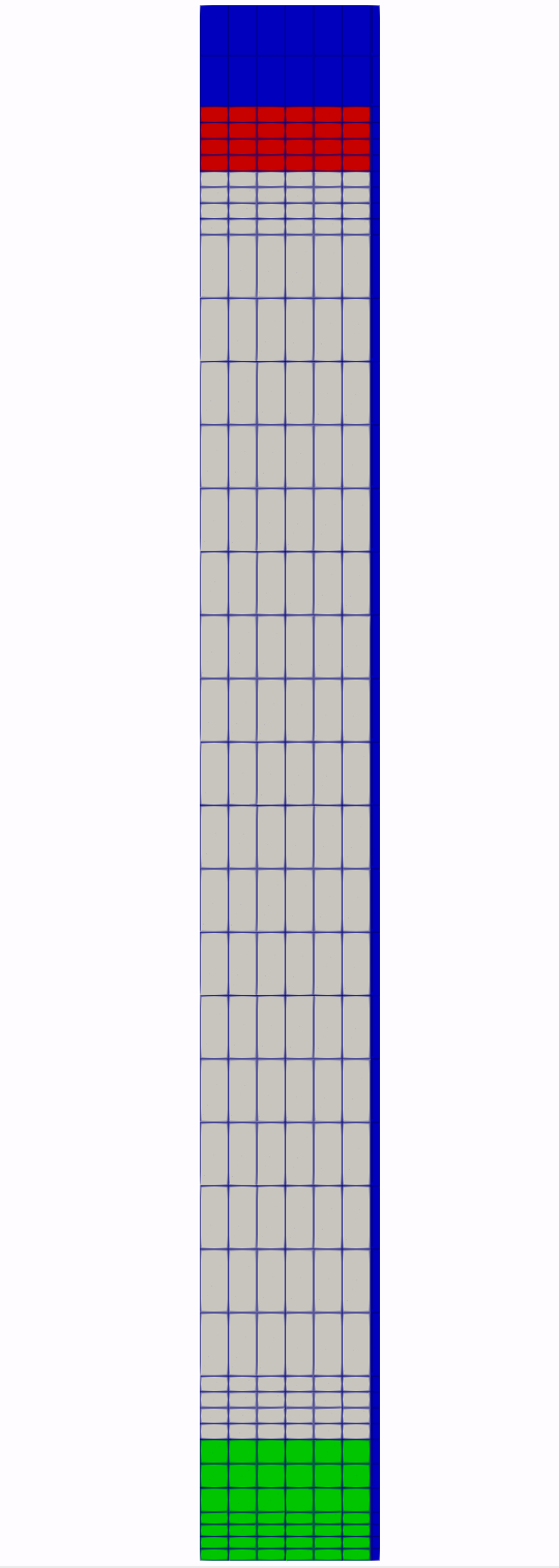
Figure 1: Mesh for Step 5.

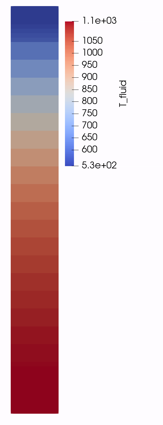
Figure 2: Temperature of the fluid for Step 5.

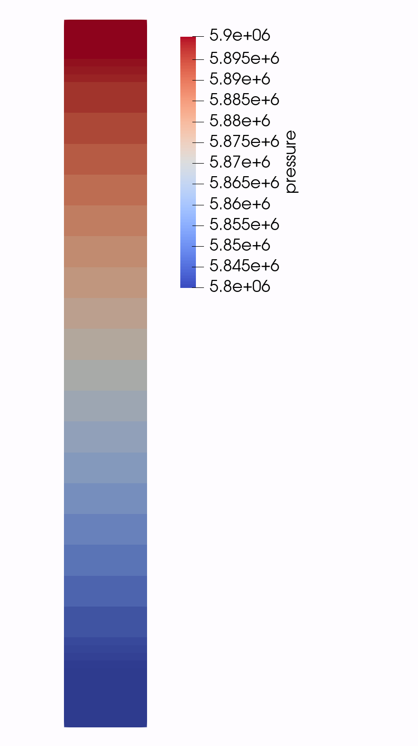
Figure 3: Pressure of the system for Step 5.

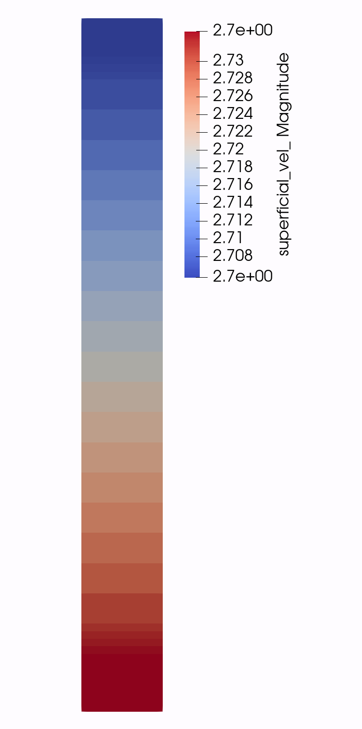
Figure 4: Fluid velocity in the system for Step 5.

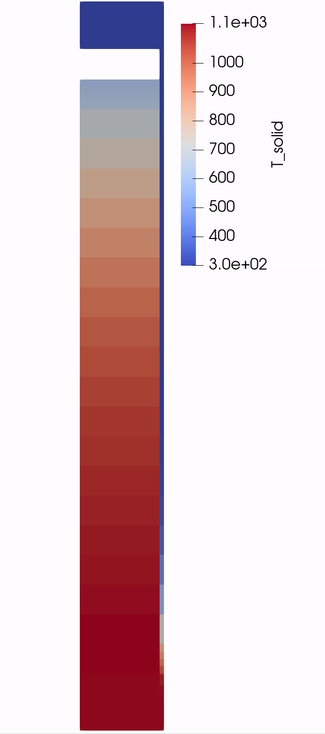
Figure 5: Temperature of the solid for Step 5.