val-2c
Test Cell Release Experiment
Case Description
This validation problem is taken from Holland and Jalbert (1986) and was part of the validation suite of TMAP4 Longhurst et al. (1992) and TMAP7 Ambrosek and Longhurst (2008). It has been updated and extended in Simon et al. (2025). Whenever tritium is released into a fusion reactor test cell, it is crucial to clean it up to prevent exposure. This case models an experiment conducted at Los Alamos National Laboratory at the tritium systems test assembly (TSTA) to study the behavior of tritium once released in a test cell and the efficacy of the emergency tritium cleanup system (ETCS).
The experimental set up, described in greater detail in Holland and Jalbert (1986), can be summarized as such: the inner walls of an enclosure of volume are covered with an aluminum foil and then covered in paint with an average thickness , which is then in contact with the enclosure air. A given amount, T, of tritium, T, is injected in the enclosure, which initially contained ambient air, representing tritium release. A flow rate through the enclosure represents the air replacement time expected for large test cells. The purge gas is ambient air with 20% relative humidity. A fraction of that amount is diverted through the measurement system to determine the concentrations of chemical species within the enclosure.
Several phenomena are taking place and need to be captured in the model to determine the concentrations of elemental tritium (i.e., T and HT), tritiated water (i.e., HTO), and water (i.e., HO). First, The following chemical reactions occur inside the enclosure: (1) (2) mostly as a consequence of the tritium reactivity. The reaction rates of these reactions are and , respectively, where (3) and (4) Here, represents the concentration of species , and is a constant.
Second, the different species will permeate in the paint. The elemental tritium species, T and HT, have a given solubility and diffusivity , while the tritiated water, HTO, and water, HO, have a solubility and diffusivity . It is expected that the species will initially permeate into the paint and later get released as the purge gas cleans up the enclosure air.
The objectives of this case are to determine the time evolution of T and HTO concentrations in the enclosure, match the experimental data published in Holland and Jalbert (1986), and display this comparison with the appropriate error checking (see Figure 1 and Figure 2).
Model Description
To model the case described above, TMAP8 simulates a one-dimensional domain with one block to represent the air in the enclosure, and another block to represent the paint. In each block, the simulation tracks the local concentration of T, HT, HTO, and HO. Note that this case can easily be extended to a two- or three-dimensional case, but consistent with previous analyses, we will maintain the one-dimensional configuration here.
In the enclosure, to capture the purge gas and the chemical reactions, the concentrations evolve as (5) (6) (7) and (8) where is the concentration of HO in the incoming purge gas.
In the paint, TMAP8 captures species diffusion through (9) (10) (11) and (12)
At the interface between the enclosure air and the paint, sorption is captured in TMAP8 with Henry's law thanks to the ADInterfaceSorption / InterfaceSorption object: (13) where and are the concentrations of species in the enclosure and in the paint, respectively, and is the solubility (either or ). The boundary conditions are set to "no flux" since no permeation happens at the interface between the paint and the aluminum foil and the only flux leaving the enclosure is already captured by the purge gas (Holland and Jalbert, 1986).
One of the assumptions made in the original paper and TMAP4 V&V case is that the tritium is immediately added to the enclosure (Holland and Jalbert, 1986; Longhurst et al., 1992). However, this leads to an early HTO peak concentration, which does not exactly match the experimental data. In Ambrosek and Longhurst (2008), TMAP7 introduces a new enclosure to account for a slower injection of tritium. Here, we model this case with two different approaches. The first approach, like (Holland and Jalbert, 1986; Longhurst et al., 1992), assumes that the entire tritium inventory is immediately injected in the enclosure at the beginning of the experiment. The second approach assumes that the tritium inventory is being injected into the enclosure at a linear rate during a period of time until the entire tritium inventory is injected. The results of these two approaches are presented and discussed below.
Case and Model Parameters
The case and model parameters used in both approaches in TMAP8 are listed in Table 1. Some of the parameters are directly leveraged from Holland and Jalbert (1986), Longhurst et al. (1992), and Ambrosek and Longhurst (2008), but others were adapted, originally by hand (see Table 1) and then using a rigorous calibration study (see Table 2), to better match the experimental data.
Table 1: Case and model parameters values used in both immediate and delayed injection approaches in TMAP8 with , the gas constant, and , Avogadro's number, as defined in PhysicalConstants. When values are the same for both approaches, they are noted as identical. Model parameters that have been adapted from Longhurst et al. (1992) show a corrective factor in bold. Units are converted in the input file.
| Parameter | Immediate injection approach | Delayed injection approach | Unit | Reference |
|---|---|---|---|---|
| 0.96 | Identical | m | Holland and Jalbert (1986) | |
| 0.16 (between 0.1 and 0.2) | Identical | mm | Holland and Jalbert (1986) | |
| T | 10 | Identical | Ci/m | Holland and Jalbert (1986) |
| 714 | Identical | Pa | Longhurst et al. (1992) | |
| 0.54 | Identical | m/hr | Holland and Jalbert (1986) | |
| 303 | Identical | K | Holland and Jalbert (1986) | |
| Total time | 180000 | Identical | s | Holland and Jalbert (1986) |
| m/Ci/s | Adapted from Longhurst et al. (1992) | |||
| 4.0 | Identical | m/s | Holland and Jalbert (1986) | |
| 1.0 | Identical | m/s | Holland and Jalbert (1986) | |
| 1/m/Pa | Adapted from Longhurst et al. (1992) | |||
| 1/m/Pa | Adapted from Longhurst et al. (1992) | |||
| N/A | 3 | hr |
The calibration study was performed using MOOSE's stochastic tools module, and in particular the Parallel Subset Simulation (PSS) approach. The inputs and methodology provided here do not correspond to the full PSS study, but a scaled down version of it to minimize the computational costs. For this PSS study, we used 5 subsets with a subset probability of 0.1 (default) and 1000 samples per subset for a total of 5000 simulations, which were performed in parallel on 5 processors. For a full PSS study, it is common to use 10 subsets with 10000 samples per subset.
To calibrate the model against both the T and HTO concentrations in the enclosure over time, we performed a multi-objective optimization study. The penalties for the difference between the experimental data and the modeling prediction is given by
(14)
for HTO, and
(15)
for T. The metric to be optimized is then defined as the time integral of
(16)
Notably, the integral difference is defined in logarithmic space to give equal weight to all data points in the logarithmic scale during the optimization process. The complexity of the optimization metric is due to the large difference in scale for each species, as well as the discrete nature of the T measurements compared to the almost continuous nature of the HTO measurements. These differences make it challenging to optimize the fits of both species.
The comparison between the original and calibrated values of selected model parameters is summarized in Table 2.
Table 2: Calibrated model parameters values for the delayed injection case in val-2c..
| Parameter | Non-calibrated values (see Table 1) | Calibrated values using Parallel Subset Simulation | Unit |
|---|---|---|---|
| 2.833 | m/Ci/s | ||
| 4.0 | 3.864 | m/s | |
| 1.0 | 1.737 | m/s | |
| 2.514 | 1/m/Pa | ||
| 9.862 | 1/m/Pa | ||
| 10800 | 9536 | s |
Results and Discussion
The results presented here are updated results from those presented in Simon et al. (2025). First, the initial time step was reduced from dt=60 s in Simon et al. (2025) to dt=1 s in the current case. This slightly affects the results for both the immediate and delayed injection cases. However, the results are qualitatively unchanged and conclusions remain valid. Second, the calibration approach was updated since Simon et al. (2025) with an updated multi-objective function, and new results. This improves the previous calibration results from Simon et al. (2025).
Figure 1 and Figure 2 show the comparison of the TMAP8 calculations (both with immediately injected and delayed injected T) against the experimental data for T and HTO concentration in the enclosure over time. There is reasonable agreement between the TMAP8 predictions and the experimental data. In the case of immediate T injection, the root mean square percentage errors (RMSPE) are equal to RMSPE = 58.68% for T and RMSPE = 146.23% for HTO, respectively. When accounting for a delay in T injection, the TMAP8 predictions best match the experimental data, in particular the position of the peak HTO concentration. The RMSPE values decrease to RMSPE = 89.50% for T and RMSPE = 75.66% for HTO, respectively. Note that the model parameters listed in Table 1 are somewhat different from Holland and Jalbert (1986), Longhurst et al. (1992), and Ambrosek and Longhurst (2008) to better match the experimental data. In particular, Longhurst et al. (1992) and Ambrosek and Longhurst (2008) did not validate the TMAP predictions against T concentration, which we do here in Figure 1 and in Simon et al. (2025). This affects some of the model parameters.
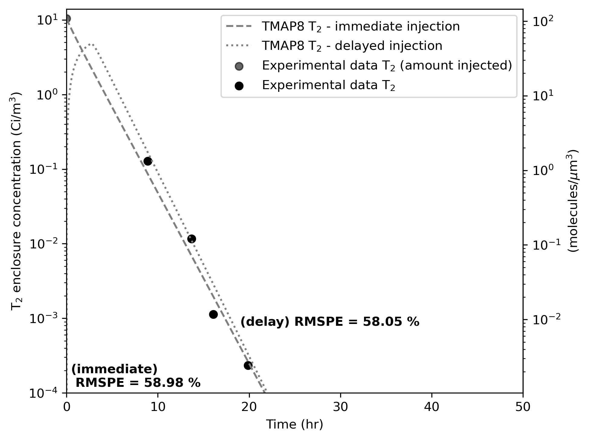
Figure 1: Comparison of TMAP8 calculations against the experimental data for T concentration in the enclosure over time. TMAP8 matches the experimental data well, with an improvement when T is injected over a given period rather than immediately. Calibration of the delayed injection model delivers further improvements.
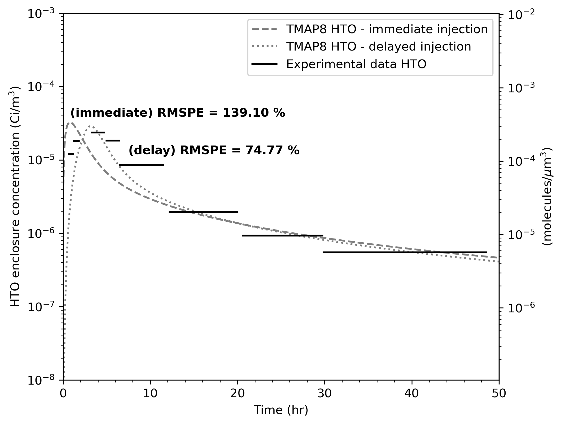
Figure 2: Comparison of TMAP8 calculations against the experimental data for HTO concentration in the enclosure over time. Calibration of the delayed injection model delivers further improvements, with more accurate simulation results when T is injected over a given period rather than immediately.
As shown in the red curve in Figure 1 and Figure 2, using MOOSE's stochastic tools module notably increased the agreement between the modeling predictions and experimental data for both the T and HTO concentrations. The RMSPE for T decreases from 89.50% to 30.18% and the RMSPE for HTO decreases from 75.66% to 67.07%. Note that although the calibration approach is similar to the one presented in Simon et al. (2025), the results presented here include more simulations and the quality of the calibration is increased here (RMSPE values are further decreased here).
Figure 3 and Figure 4 show the evolution of the model parameter values and of the optimization metric (time integral of defined in Eq. (16)) as a function of the number of simulation. The calibrated model corresponds to the highest value.
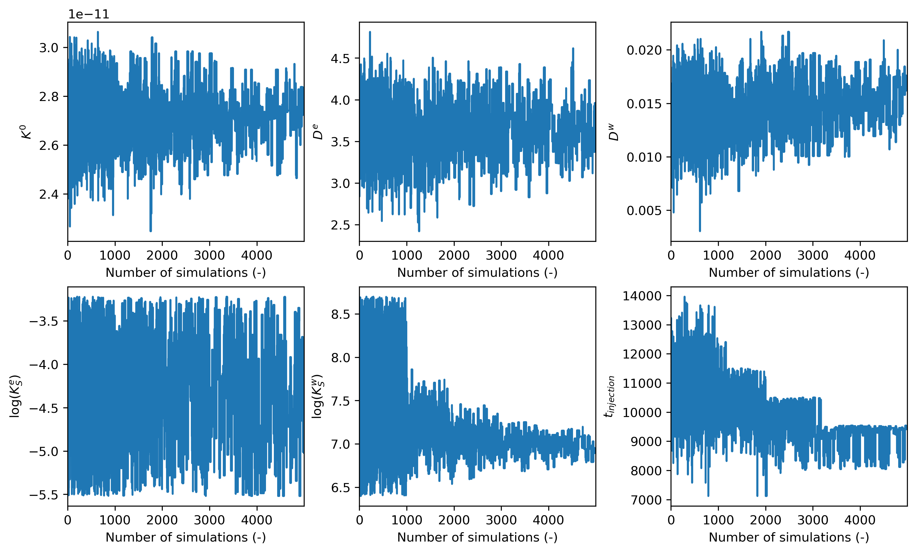
Figure 3: Evolution of the model parameter values as a function of the number of simulations.
![Evolution of the optimization metric (time integral of $g$ defined in [eq:optimization_metric]) as a function of the number of simulations. The calibrated model corresponds to the highest value.](figures/val-2c_pss_output.png)
Figure 4: Evolution of the optimization metric (time integral of defined in Eq. (16)) as a function of the number of simulations. The calibrated model corresponds to the highest value.
Figure 5 and Figure 6 show the value of the calibrated parameters and the range of the data that was explored in the Parallel Subset Simulation study. Figure 5 shows the parameters that followed a normal distribution, and Figure 6 shows those that followed a uniform distribution in log scale. In both cases, the calibrated parameters are not on the extremes of the distribution, suggesting that the ranges were properly defined.
 study. None of the parameters are at the extremes of the distribution.](figures/val-2c_pss_inputs_normal_calibrated.png)
Figure 5: Calibrated parameter values compared to the normalized normal distribution used in the Parallel Subset Simulation study. None of the parameters are at the extremes of the distribution.
 study. None of the parameters are at the extremes of the distributions.](figures/val-2c_pss_inputs_uniform_calibrated.png)
Figure 6: Calibrated parameter values compared to the normal distribution in the log scale used in the Parallel Subset Simulation study. None of the parameters are at the extremes of the distributions.
Input files
The input files for this case can be found at (test/tests/val-2c/val-2c_immediate_injection.i) and (test/tests/val-2c/val-2c_delay.i). Note that both input files utilize a common base file (test/tests/val-2c/val-2c_base.i) with the line !include val-2c_base.i. The base input file contains all the features and TMAP8 objects common to both cases, reducing duplication, and this allows the immediate injection and delayed injection inputs to focus on what is specific to each case. Note that both input files are also used as TMAP8 tests, outlined at (test/tests/val-2c/tests).
To learn more about the !include feature, refer to the Input File Syntax page.
For the calibration study, additional input files are provided.
(test/tests/val-2c/val-2c_base_pss.i) provides key functions and postprocessor blocks necessary for the PSS study, including calculations of the multi-objective optimization metric (i.e., the time integral of defined in Eq. (16)).
(test/tests/val-2c/val-2c_delay_pss.i) includes both (test/tests/val-2c/val-2c_base_pss.i) and (test/tests/val-2c/val-2c_delay.i) to generate the needed full input file for the simulation.
(test/tests/val-2c/val-2c_pss_main.i) is the main input file for the PSS study. It defines what model parameters to vary and how, defines what approach to use, and initiates simulations using (test/tests/val-2c/val-2c_delay_pss.i).
To run the PSS study in the terminal, users can perform:
cd ~/projects/TMAP8/test/tests/val-2c/
mpirun -np 5 ~/projects/TMAP8/tmap8-opt -i val-2c_pss_main.i
Note that this study is time consuming since a large number of simulations are being run. Modifying the PSS parameters can reduce the computational cost.
Although a very short PSS study is simulated as a test in (test/tests/val-2c/tests) to ensure these files run properly, the full calibration study is not performed regularly in tests to limit computational costs within the TMAP8 testing suite. The gold files (test/tests/val-2c/gold/val-2c_pss_results/val-2c_pss_main_out.json) and (test/tests/val-2c/gold/calibrated_parameter_values.txt) are, therefore, not continuously tested, and the calibrated model parameters used in (test/tests/val-2c/tests) are not continuously updated.
References
- James Ambrosek and GR Longhurst.
Verification and Validation of TMAP7.
Technical Report INEEL/EXT-04-01657, Idaho National Engineering and Environmental Laboratory, December 2008.[BibTeX]
@techreport{ambrosek2008verification, author = "Ambrosek, James and Longhurst, GR", title = "{Verification and Validation of TMAP7}", year = "2008", number = "INEEL/EXT-04-01657", month = "December", institution = "Idaho National Engineering and Environmental Laboratory" } - D F Holland and R A Jalbert.
A model for tritium concentration following tritium release into a test cell and subsequent operation of an atmospheric cleanup system.
In Eleventh Symposium on Fusion Engineering. IEEE Cat. No. CH2251-7, Vol 1. pp. 638-643, 11 1986.[BibTeX]
@inproceedings{Holland1986, author = "Holland, D F and Jalbert, R A", city = "Austin, TX", booktitle = "Eleventh Symposium on Fusion Engineering", month = "11", publisher = "IEEE Cat. No. CH2251-7, Vol 1. pp. 638-643", title = "A model for tritium concentration following tritium release into a test cell and subsequent operation of an atmospheric cleanup system", year = "1986" } - GR Longhurst, SL Harms, ES Marwil, and BG Miller.
Verification and Validation of TMAP4.
Technical Report EGG-FSP-10347, Idaho National Engineering Laboratory, Idaho Falls, ID (United States), 1992.[BibTeX]
@techreport{longhurst1992verification, author = "Longhurst, GR and Harms, SL and Marwil, ES and Miller, BG", title = "{Verification and Validation of TMAP4}", year = "1992", institution = "Idaho National Engineering Laboratory, Idaho Falls, ID (United States)", number = "EGG-FSP-10347" } - Pierre-Clément A. Simon, Casey T. Icenhour, Gyanender Singh, Alexander D Lindsay, Chaitanya Vivek Bhave, Lin Yang, Adriaan Anthony Riet, Yifeng Che, Paul Humrickhouse, Masashi Shimada, and Pattrick Calderoni.
MOOSE-based tritium migration analysis program, version 8 (TMAP8) for advanced open-source tritium transport and fuel cycle modeling.
Fusion Engineering and Design, 214:114874, May 2025.
doi:10.1016/j.fusengdes.2025.114874.[BibTeX]
@article{Simon2025,
    author = "Simon, Pierre-Clément A. and Icenhour, Casey T. and Singh, Gyanender and Lindsay, Alexander D and Bhave, Chaitanya Vivek and Yang, Lin and Riet, Adriaan Anthony and Che, Yifeng and Humrickhouse, Paul and Shimada, Masashi and Calderoni, Pattrick",
    title = "{MOOSE}-based Tritium Migration Analysis Program, Version 8 ({TMAP8}) for Advanced Open-Source Tritium Transport and Fuel Cycle Modeling",
    journal = "Fusion Engineering and Design",
    publisher = "Elsevier",
    volume = "214",
    pages = "114874",
    year = "2025",
    month = "May",
    issn = "0920-3796",
    doi = "10.1016/j.fusengdes.2025.114874"
}
(test/tests/val-2c/val-2c_immediate_injection.i)
# This input file utilizes val_2c_base and adds specific parameter values and capabilities to inject T2 immediately

# Physical Constants (from PhysicalConstant.h)
kb = '${units 1.380649e-23 J/K}' # Boltzmann constant based on number used in include/utils/PhysicalConstants.h
NA = '${units 6.02214076e23 at/mol}' # Avogadro's number based on number used in include/utils/PhysicalConstants.h

## Geometry
paint_thickness = '${units 0.16 mm -> mum}'
mesh_num_nodes_paint = 12 # impose by manual mesh
mesh_node_size_paint = '${fparse paint_thickness/mesh_num_nodes_paint}'
length_domain = '${fparse paint_thickness + 2*mesh_node_size_paint}'
volume_enclosure = '${units 0.96 m^3 -> mum^3}'

## Conditions
temperature = '${units 303 K}'

## Conversion
Curie = '${units 3.7e10 1/s}' # desintegrations/s - activity of one Curie
decay_rate_tritium = '${units 1.78199e-9 1/s/at}' # desintegrations/s/atoms
conversion_Ci_atom = '${units ${fparse decay_rate_tritium / Curie} 1/at}' # 1 tritium at = ~4.82e-20 Ci
concentration_to_pressure_conversion_factor = '${units ${fparse kb * temperature} Pa*m^3 -> Pa*mum^3}' # J = Pa*m^3

## Material properties
diffusivity_elemental_tritium = '${units 4.0e-12 m^2/s -> mum^2/s}'
diffusivity_tritiated_water = '${units 1.0e-14 m^2/s -> mum^2/s}'
diffusivity_artificial_enclosure = '${fparse diffusivity_elemental_tritium*1e3}'
reaction_rate = '${units ${fparse 1.5 * 2.0e-10*conversion_Ci_atom} m^3/at/s -> mum^3/at/s}' # ~ 1.5* 9.62e-30 m^3/at/s, close to the 1.0e-29 m3/atoms/s in TMAP4
solubility_elemental_tritium = '${units ${fparse 5e-2 * 4.0e19} 1/m^3/Pa -> 1/mum^3/Pa}' # molecules/microns^3/Pa = molecules*s^2/m^2/kg
solubility_tritiated_water = '${units ${fparse 3.5e-4 * 6.0e24} 1/m^3/Pa -> 1/mum^3/Pa}' # molecules/microns^3/Pa = molecules*s^2/m^2/kg

## Initial conditions
# The units below are actually in molecules, not atoms
initial_T2_inventory = '${units ${fparse 10 / 2 / conversion_Ci_atom} at}' # (equivalent to 10 Ci) - the 1/2 is to account for 2 tritium atoms per molecules, both contributing to activity
initial_T2_concentration = '${units ${fparse initial_T2_inventory / volume_enclosure} at/mum^3}'
initial_H2O_pressure = '${units 714 Pa}' # Found in TMAP4 input file, which corresponds to ambient air with 20% relative humidity.
initial_H2O_concentration = '${units ${fparse initial_H2O_pressure / concentration_to_pressure_conversion_factor} at/mum^3}'

## Numerical parameters
time_step = '${units 1 s}'
time_end = '${units 180000 s}'
dtmax = '${units 1e3 s}'
dtmin = '${units 1 s}'
lower_value_threshold = '${units -1e-20 at/mum^3}' # lower limit for concentration

## Inflow and outflow
inflow = '${units 0.54 m^3/h -> mum^3/s}' # inflow of normally moist (20% relative humidity) air at the same temperature as the enclosure
inflow_concentration = '${fparse initial_H2O_concentration * inflow / volume_enclosure}'
outflow = '${units 0.54 m^3/h -> mum^3/s}' # outflow of enclosure air # even if only 0.06 m^3/h is used to do measurements, all that air is purged out.

!include val-2c_base.i

[Variables]
  # T2 concentration in the enclosure in molecules/microns^3
  [t2_enclosure_concentration]
    initial_condition = ${initial_T2_concentration}
  []
[]
(test/tests/val-2c/val-2c_delay.i)
# This input file utilizes val_2c_base and adds specific parameter values and capabilities to inject T2 with a delay

!include val-2c_delay.params
!include val-2c_base.i

[Functions]
  [injection_window]
    type = ParsedFunction
    expression = 'if(t<${time_injection_T2_start}, 0., if(t<${time_injection_T2_end}, ${injection_rate_T2}, 0.))'
  []
[]

[Kernels]
  [t2_inflow]
    type = MaskedBodyForce
    variable = t2_enclosure_concentration
    value = '1'
    function = 'injection_window'
    mask = '1'
    block = 1
  []
[]
(test/tests/val-2c/val-2c_base.i)
# Validation problem #2c from TMAP4/TMAP7 V&V document
# Test Cell Release Experiment based on
# D. F. Holland and R. A. Jalbert, "A Model for Tritium Concentration Following Tritium
# Release into a Test Cell and Subsequent Operation of an Atmospheric Cleanup Systen,"
# Proceedings, Eleventh Symposium of Fusion Engineering, November 18-22, 1985,. Austin,
# TX, Vol I, pp. 638-43, IEEE Cat. No. CH2251-7.

# Note that the approach to model this validation case is different in TMAP4 and TMAP7.

[Mesh]
  [base_mesh]
    type = GeneratedMeshGenerator
    dim = 1
    nx = '${fparse mesh_num_nodes_paint + 2}'
    xmax = ${length_domain}
  []
  [subdomain_id]
    input = base_mesh
    type = SubdomainPerElementGenerator
    subdomain_ids = '0 0 0 0 0 0 0 0 0 0 0 0 1 1'
  []
  [interface]
    type = SideSetsBetweenSubdomainsGenerator
    input = subdomain_id
    primary_block = '0' # paint
    paired_block = '1' # enclosure
    new_boundary = 'interface'
  []
  [interface_other_side]
    type = SideSetsBetweenSubdomainsGenerator
    input = interface
    primary_block = '1' # enclosure
    paired_block = '0' # paint
    new_boundary = 'interface_other'
  []
[]

[Variables]
  # T2 concentration in the enclosure in molecules/microns^3
  [t2_enclosure_concentration]
    block = 1
  []
  # HT concentration in the enclosure in molecules/microns^3
  [ht_enclosure_concentration]
    block = 1
  []
  # HTO concentration in the enclosure in molecules/microns^3
  [hto_enclosure_concentration]
    block = 1
  []
  # H2O concentration in the enclosure in molecules/microns^3
  [h2o_enclosure_concentration]
    block = 1
    initial_condition = ${initial_H2O_concentration}
  []
  # concentration of T2 in the paint in molecules/microns^3
  [t2_paint_concentration]
    block = 0
  []
  # concentration of HT in the paint in molecules/microns^3
  [ht_paint_concentration]
    block = 0
  []
  # concentration of HTO in the paint in molecules/microns^3
  [hto_paint_concentration]
    block = 0
  []
  # concentration of H2O in the paint in molecules/microns^3
  [h2o_paint_concentration]
    block = 0
  []
[]

[AuxVariables]
  # Used to prevent negative concentrations
  [bounds_dummy_t2_paint_concentration]
    order = FIRST
    family = LAGRANGE
  []
  [bounds_dummy_t2_enclosure_concentration]
    order = FIRST
    family = LAGRANGE
  []
  [bounds_dummy_hto_paint_concentration]
    order = FIRST
    family = LAGRANGE
  []
  [bounds_dummy_hto_enclosure_concentration]
    order = FIRST
    family = LAGRANGE
  []
  [bounds_dummy_h2o_paint_concentration]
    order = FIRST
    family = LAGRANGE
  []
  [bounds_dummy_h2o_enclosure_concentration]
    order = FIRST
    family = LAGRANGE
  []
[]

[Bounds]
  # To prevent negative concentrations
  [t2_paint_concentration_lower_bound]
    type = ConstantBounds
    variable = bounds_dummy_t2_paint_concentration
    bounded_variable = t2_paint_concentration
    bound_type = lower
    bound_value = ${lower_value_threshold}
  []
  [t2_enclosure_concentration_lower_bound]
    type = ConstantBounds
    variable = bounds_dummy_t2_enclosure_concentration
    bounded_variable = t2_enclosure_concentration
    bound_type = lower
    bound_value = ${lower_value_threshold}
  []
  [hto_paint_concentration_lower_bound]
    type = ConstantBounds
    variable = bounds_dummy_hto_paint_concentration
    bounded_variable = hto_paint_concentration
    bound_type = lower
    bound_value = ${lower_value_threshold}
  []
  [hto_enclosure_concentration_lower_bound]
    type = ConstantBounds
    variable = bounds_dummy_hto_enclosure_concentration
    bounded_variable = hto_enclosure_concentration
    bound_type = lower
    bound_value = ${lower_value_threshold}
  []
  [h2o_paint_concentration_lower_bound]
    type = ConstantBounds
    variable = bounds_dummy_h2o_paint_concentration
    bounded_variable = h2o_paint_concentration
    bound_type = lower
    bound_value = -1e-4
  []
  [h2o_enclosure_concentration_lower_bound]
    type = ConstantBounds
    variable = bounds_dummy_h2o_enclosure_concentration
    bounded_variable = h2o_enclosure_concentration
    bound_type = lower
    bound_value = -1e-4
  []
[]

[Kernels]
  # In the enclosure
  [t2_time_derivative]
    type = TimeDerivative
    variable = t2_enclosure_concentration
    block = 1
  []
  [t2_outflow]
    type = MaskedBodyForce
    variable = t2_enclosure_concentration
    value = '-1'
    mask = t2_enclosure_concentration_outflow
    block = 1
  []
  [t2_diffusion]
    type = MatDiffusion
    variable = t2_enclosure_concentration
    block = 1
    diffusivity = ${diffusivity_artificial_enclosure}
  []
  [ht_time_derivative]
    type = TimeDerivative
    variable = ht_enclosure_concentration
    block = 1
  []
  [ht_outflow]
    type = MaskedBodyForce
    variable = ht_enclosure_concentration
    value = '-1'
    mask = ht_enclosure_concentration_outflow
    block = 1
  []
  [ht_diffusion]
    type = MatDiffusion
    variable = ht_enclosure_concentration
    block = 1
    diffusivity = ${diffusivity_artificial_enclosure}
  []
  [hto_time_derivative]
    type = TimeDerivative
    variable = hto_enclosure_concentration
    block = 1
  []
  [hto_outflow]
    type = MaskedBodyForce
    variable = hto_enclosure_concentration
    value = '-1'
    mask = hto_enclosure_concentration_outflow
    block = 1
  []
  [hto_diffusion]
    type = MatDiffusion
    variable = hto_enclosure_concentration
    block = 1
    diffusivity = ${diffusivity_artificial_enclosure}
  []
  [h2o_time_derivative]
    type = TimeDerivative
    variable = h2o_enclosure_concentration
    block = 1
  []
  [h2o_inflow]
    type = MaskedBodyForce
    variable = h2o_enclosure_concentration
    mask = ${inflow_concentration}
    block = 1
  []
  [h2o_outflow]
    type = MaskedBodyForce
    variable = h2o_enclosure_concentration
    value = '-1'
    mask = h2o_enclosure_concentration_outflow
    block = 1
  []
  [h2o_diffusion]
    type = MatDiffusion
    variable = h2o_enclosure_concentration
    block = 1
    diffusivity = ${diffusivity_artificial_enclosure}
  []

  # reaction T2+H2O->HTO+HT
  [reaction_1_t2]
    type = ADMatReactionFlexible
    variable = t2_enclosure_concentration
    block = 1
    coeff = -1
    reaction_rate_name = reaction_rate_t2
  []
  [reaction_1_h2o]
    type = ADMatReactionFlexible
    variable = h2o_enclosure_concentration
    block = 1
    coeff = -1
    reaction_rate_name = reaction_rate_t2
  []
  [reaction_1_hto]
    type = ADMatReactionFlexible
    variable = hto_enclosure_concentration
    block = 1
    coeff = 1
    reaction_rate_name = reaction_rate_t2
  []
  [reaction_1_ht]
    type = ADMatReactionFlexible
    variable = ht_enclosure_concentration
    block = 1
    coeff = 1
    reaction_rate_name = reaction_rate_t2
  []
  # reaction HT+H2O->HTO+H2
  [reaction_2_HT]
    type = ADMatReactionFlexible
    variable = ht_enclosure_concentration
    block = 1
    coeff = -1
    reaction_rate_name = reaction_rate_ht
  []
  [reaction_2_h2o]
    type = ADMatReactionFlexible
    variable = h2o_enclosure_concentration
    block = 1
    coeff = -1
    reaction_rate_name = reaction_rate_ht
  []
  [reaction_2_hto]
    type = ADMatReactionFlexible
    variable = hto_enclosure_concentration
    block = 1
    coeff = 1
    reaction_rate_name = reaction_rate_ht
  []

  # In the paint
  [t2_paint_time]
    type = TimeDerivative
    variable = t2_paint_concentration
    block = 0
  []
  [t2_paint_diffusion]
    type = MatDiffusion
    variable = t2_paint_concentration
    block = 0
    diffusivity = '${diffusivity_elemental_tritium}'
  []
  [ht_paint_time]
    type = TimeDerivative
    variable = ht_paint_concentration
    block = 0
  []
  [ht_paint_diffusion]
    type = MatDiffusion
    variable = ht_paint_concentration
    block = 0
    diffusivity = '${diffusivity_elemental_tritium}'
  []
  [hto_paint_time]
    type = TimeDerivative
    variable = hto_paint_concentration
    block = 0
  []
  [hto_paint_diffusion]
    type = MatDiffusion
    variable = hto_paint_concentration
    block = 0
    diffusivity = '${diffusivity_tritiated_water}'
  []
  [h2o_paint_time]
    type = TimeDerivative
    variable = h2o_paint_concentration
    block = 0
  []
  [h2o_paint_diffusion]
    type = MatDiffusion
    variable = h2o_paint_concentration
    block = 0
    diffusivity = '${diffusivity_tritiated_water}'
  []
[]

[InterfaceKernels]
  # solubility at the surface of the paint
  [t2_solubility]
    type = ADInterfaceSorption
    variable = t2_paint_concentration
    neighbor_var = t2_enclosure_concentration # molecules/microns^3
    unit_scale_neighbor = '${fparse 1e18/NA}' # to convert neighbor concentration to mol/m^3
    K0 = ${solubility_elemental_tritium}
    Ea = 0
    n_sorption = 1 # Henry's law
    temperature = ${temperature}
    diffusivity = diffusivity_elemental_tritium
    boundary = 'interface'
  []
  [ht_solubility]
    type = ADInterfaceSorption
    variable = ht_paint_concentration
    neighbor_var = ht_enclosure_concentration # molecules/microns^3
    unit_scale_neighbor = '${fparse 1e18/NA}' # to convert neighbor concentration to mol/m^3
    K0 = ${solubility_elemental_tritium}
    Ea = 0
    n_sorption = 1 # Henry's law
    temperature = ${temperature}
    diffusivity = diffusivity_elemental_tritium
    boundary = 'interface'
  []
  [hto_solubility]
    type = ADInterfaceSorption
    variable = hto_paint_concentration
    neighbor_var = hto_enclosure_concentration # molecules/microns^3
    unit_scale_neighbor = '${fparse 1e18/NA}' # to convert neighbor concentration to mol/m^3
    K0 = ${solubility_tritiated_water}
    Ea = 0
    n_sorption = 1 # Henry's law
    temperature = ${temperature}
    diffusivity = diffusivity_tritiated_water
    boundary = 'interface'
  []
  [h2o_solubility]
    type = ADInterfaceSorption
    variable = h2o_paint_concentration
    neighbor_var = h2o_enclosure_concentration # molecules/microns^3
    unit_scale_neighbor = '${fparse 1e18/NA}' # to convert neighbor concentration to mol/m^3
    K0 = ${solubility_tritiated_water}
    Ea = 0
    n_sorption = 1 # Henry's law
    temperature = ${temperature}
    diffusivity = diffusivity_tritiated_water
    boundary = 'interface'
  []
[]

[Materials]
  [reaction_rate_t2]
    type = ADDerivativeParsedMaterial
    coupled_variables = 't2_enclosure_concentration ht_enclosure_concentration hto_enclosure_concentration'
    expression = '${reaction_rate} * 2 * t2_enclosure_concentration * (2*t2_enclosure_concentration + ht_enclosure_concentration + hto_enclosure_concentration)'
    property_name = reaction_rate_t2
    block = 1
  []
  [reaction_rate_ht]
    type = ADDerivativeParsedMaterial
    coupled_variables = 't2_enclosure_concentration ht_enclosure_concentration hto_enclosure_concentration'
    expression = '${reaction_rate} * ht_enclosure_concentration * (2*t2_enclosure_concentration + ht_enclosure_concentration + hto_enclosure_concentration)'
    property_name = reaction_rate_ht
    block = 1
  []
  [diffusivity_elemental_tritium_paint]
    type = ADConstantMaterial
    value = ${diffusivity_elemental_tritium}
    property_name = 'diffusivity_elemental_tritium'
    block = 0
  []
  [diffusivity_elemental_tritium_enclosure]
    type = ADConstantMaterial
    value = ${diffusivity_artificial_enclosure}
    property_name = 'diffusivity_elemental_tritium'
    block = 1
  []
  [diffusivity_tritiated_water_paint]
    type = ADConstantMaterial
    value = ${diffusivity_tritiated_water}
    property_name = 'diffusivity_tritiated_water'
    block = 0
  []
  [diffusivity_tritiated_water_enclosure]
    type = ADConstantMaterial
    value = ${diffusivity_artificial_enclosure}
    property_name = 'diffusivity_tritiated_water'
    block = 1
  []

  [t2_enclosure_concentration_outflow]
    type = DerivativeParsedMaterial
    coupled_variables = 't2_enclosure_concentration'
    expression = 't2_enclosure_concentration * ${outflow} / ${volume_enclosure}'
    property_name = 't2_enclosure_concentration_outflow'
    block = 1
  []
  [ht_enclosure_concentration_outflow]
    type = DerivativeParsedMaterial
    coupled_variables = 'ht_enclosure_concentration'
    expression = 'ht_enclosure_concentration * ${outflow} / ${volume_enclosure}'
    property_name = 'ht_enclosure_concentration_outflow'
    block = 1
  []
  [hto_enclosure_concentration_outflow]
    type = DerivativeParsedMaterial
    coupled_variables = 'hto_enclosure_concentration'
    expression = 'hto_enclosure_concentration * ${outflow} / ${volume_enclosure}'
    property_name = 'hto_enclosure_concentration_outflow'
    block = 1
  []
  [h2o_enclosure_concentration_outflow]
    type = DerivativeParsedMaterial
    coupled_variables = 'h2o_enclosure_concentration'
    expression = 'h2o_enclosure_concentration * ${outflow} / ${volume_enclosure}'
    property_name = 'h2o_enclosure_concentration_outflow'
    block = 1
  []
[]

[Postprocessors]
  # Pressures in enclosure
  [t2_enclosure_edge_concentration] # (molecules/microns^3)
    type = PointValue
    point = '${length_domain} 0 0' # on the far side of the enclosure
    variable = t2_enclosure_concentration
    execute_on = 'initial timestep_end'
  []
  [ht_enclosure_edge_concentration] # (molecules/microns^3)
    type = PointValue
    point = '${length_domain} 0 0' # on the far side of the enclosure
    variable = ht_enclosure_concentration
    execute_on = 'initial timestep_end'
  []
  [hto_enclosure_edge_concentration] # (molecules/microns^3)
    type = PointValue
    point = '${length_domain} 0 0' # on the far side of the enclosure
    variable = hto_enclosure_concentration
    execute_on = 'initial timestep_end'
  []
  [h2o_enclosure_edge_concentration] # (molecules/microns^3)
    type = PointValue
    point = '${length_domain} 0 0' # on the far side of the enclosure
    variable = h2o_enclosure_concentration
    execute_on = 'initial timestep_end'
  []

  # Inventory in enclosure
  [t2_enclosure_inventory] # (molecules/microns^2)
    type = ElementIntegralVariablePostprocessor
    variable = t2_enclosure_concentration
    execute_on = 'initial timestep_end'
    block = 1
  []
  [ht_enclosure_inventory] # (molecules/microns^2)
    type = ElementIntegralVariablePostprocessor
    variable = ht_enclosure_concentration
    execute_on = 'initial timestep_end'
    block = 1
  []
  [hto_enclosure_inventory] # (molecules/microns^2)
    type = ElementIntegralVariablePostprocessor
    variable = hto_enclosure_concentration
    execute_on = 'initial timestep_end'
    block = 1
  []
  [h2o_enclosure_inventory] # (molecules/microns^2)
    type = ElementIntegralVariablePostprocessor
    variable = h2o_enclosure_concentration
    execute_on = 'initial timestep_end'
    block = 1
  []

  # Inventory in paint
  [t2_paint_inventory] # (molecules/microns^2)
    type = ElementIntegralVariablePostprocessor
    variable = t2_paint_concentration
    execute_on = 'initial timestep_end'
    block = 0
  []
  [ht_paint_inventory] # (molecules/microns^2)
    type = ElementIntegralVariablePostprocessor
    variable = ht_paint_concentration
    execute_on = 'initial timestep_end'
    block = 0
  []
  [hto_paint_inventory] # (molecules/microns^2)
    type = ElementIntegralVariablePostprocessor
    variable = hto_paint_concentration
    execute_on = 'initial timestep_end'
    block = 0
  []
  [h2o_paint_inventory] # (molecules/microns^2)
    type = ElementIntegralVariablePostprocessor
    variable = h2o_paint_concentration
    execute_on = 'initial timestep_end'
    block = 0
  []

  [tritium_total_inventory]
    type = LinearCombinationPostprocessor
    pp_names = 't2_enclosure_inventory ht_enclosure_inventory hto_enclosure_inventory t2_paint_inventory ht_paint_inventory hto_paint_inventory'
    pp_coefs = '2                      1                      1                       2                  1                  1'
    execute_on = 'initial timestep_end'
  []
[]

[Debug]
  show_var_residual_norms = true
[]

[Preconditioning]
  [smp]
    type = SMP
    full = true
  []
[]

[Executioner]
  type = Transient
  solve_type = NEWTON
  scheme = 'bdf2'

  petsc_options_iname = '-pc_type -sub_pc_type -snes_type'
  petsc_options_value = 'asm      lu           vinewtonrsls' # This petsc option helps prevent negative concentrations with bounds'

  nl_rel_tol = 1.e-10
  automatic_scaling = true
  compute_scaling_once = false

  end_time = ${time_end}
  dtmax = ${dtmax}
  dtmin = ${dtmin}
  nl_max_its = 16
  [TimeStepper]
    type = IterationAdaptiveDT
    dt = ${time_step}
    optimal_iterations = 12
    iteration_window = 1
    growth_factor = 1.1
    cutback_factor = 0.7
  []
[]

[Outputs]
  perf_graph = true
  [csv]
    type = CSV
    execute_on = 'initial timestep_end'
  []
[]
(test/tests/val-2c/tests)
[Tests]
  design = 'val-2c.md'
  validation = 'val-2c.md'
  issues = '#12 #98'
  [val-2c_immediate_injection_csv]
    type = CSVDiff
    input = val-2c_immediate_injection.i
    cli_args = 'Outputs/exodus=true'
    csvdiff = val-2c_immediate_injection_csv.csv
    requirement = 'The system shall be able to model the Test Cell Release Experiment (val-2c) with immediate T2 injection.'
    max_parallel = 1 # see #200
    recover = false # see #196
  []
  [val-2c_immediate_injection_exodus]
    type = Exodiff
    input = val-2c_immediate_injection.i
    cli_args = 'Outputs/exodus=true'
    prereq = val-2c_immediate_injection_csv
    should_execute = false # this test relies on the output files from val-2c_immediate_injection_csv, so it shouldn't be run twice
    exodiff = val-2c_immediate_injection_out.e
    custom_cmp = 'val-2c_exodus.exodiff'
    requirement = 'The system shall be able to model the Test Cell Release Experiment (val-2c) with immediate T2 injection and properly compute the exodus file.'
    max_parallel = 1 # see #200
    recover = false # see #196
  []
  [val-2c_delay_csv]
    type = CSVDiff
    input = val-2c_delay.i
    cli_args = 'Outputs/exodus=true'
    csvdiff = val-2c_delay_csv.csv
    requirement = 'The system shall be able to model the Test Cell Release Experiment (val-2c) with delayed T2 injection.'
    abs_zero = 1e-8
    rel_err = 3e-5
    max_parallel = 1 # see #200
    recover = false # see #196
  []
  [val-2c_delay_exodus]
    type = Exodiff
    input = val-2c_delay.i
    cli_args = 'Outputs/exodus=true'
    prereq = val-2c_delay_csv
    should_execute = false # this test relies on the output files from val-2c_delay_csv, so it shouldn't be run twice
    exodiff = val-2c_delay_out.e
    custom_cmp = 'val-2c_exodus.exodiff'
    requirement = 'The system shall be able to model the Test Cell Release Experiment (val-2c) with delayed T2 injection and properly compute the exodus file.'
    max_parallel = 1 # see #200
    recover = false # see #196
  []
  [val-2c_delay_calibrated_csv]
    type = CSVDiff
    input = 'val-2c_delay.i'
     # the parameter values below are from gold/calibrated_parameter_values.txt
    cli_args = 'reaction_rate=2.8331901331213944e-11
                diffusivity_elemental_tritium=3.8640662435310973
                diffusivity_tritiated_water=0.017373835349450507
                log_solubility_elemental_tritium=-3.683352919815223
                log_solubility_tritiated_water=6.8938628913078555
                time_injection_T2_end=9536.239653312441
                Outputs/file_base=val-2c_delay_calibrated_out'
    csvdiff = val-2c_delay_calibrated_out.csv
    requirement = 'The system shall be able to model the Test Cell Release Experiment (val-2c) with delayed T2 injection using calibrated model parameters.'
    abs_zero = 1e-8
    rel_err = 2e-5
    max_parallel = 1 # see #200
    recover = false # see #196
    issues = '#266'
  []
  [val-2c_delay_pss_study_csv]
    type = JSONDiff
    input = val-2c_pss_main.i
    cli_args = 'num_samplessub=2
                num_subsets=1
                Samplers/sample/num_parallel_chains=1
                subset_probability=0.5
                Samplers/sample/seed=1518
                file_base_output=val-2c_pss_results_short/val-2c_pss_main_short_out'
    jsondiff = val-2c_pss_results_short/val-2c_pss_main_short_out.json
    requirement = 'The system shall be able to perform a Parallel Subset Simulation study using a model of the Test Cell Release Experiment (val-2c) with delayed T2 injection.'
    abs_zero = 1e-8
    rel_err = 1e-5
    max_parallel = 1 # see #200
    recover = false # see #196
    issues = '#266'
  []
  [val-2c_delay_comparison]
    type = RunCommand
    command = 'python3 comparison_val-2c.py'
    requirement = 'The system shall be able to generate comparison plots between simulated solutions and experimental data of validation cases val-2c, modeling a Test Cell Release Experiment.'
    required_python_packages = 'matplotlib numpy pandas scipy os json'
  []
[]
(test/tests/val-2c/val-2c_base_pss.i)
# This input file adds key blocks to the val-2c_base.i input files for the PSS study

## Conversion
lengthscale = 1e18 # ${units 1 m^3 -> mum^3}

times_measurement_HTO_start = 2440.415722 # s
times_measurement_HTO_end = 174765.6056 # s

times_measurement_T2_1 = 32003.54498 # s
times_measurement_T2_2 = 49281.50916 # s
times_measurement_T2_3 = 57804.64646 # s
times_measurement_T2_4 = 71561.68891 # s
time_measurement_T2 = 600 # s - assuming it takes 10 minutes to take the measurement
default_diff_value = 3 # value to be used as difference between modeling prediction and experimental data when experimental data is not available

[Functions]
  [experimental_data_hto] # time (s), concentrations (Ci/m^3)
    type = PiecewiseLinear
    data_file = gold/Experimental_data_HTO_concentration.csv
    scale_factor = 1
    format = columns
  []
  [experimental_data_t2] # time (s), concentrations (Ci/m^3)
    type = PiecewiseLinear
    data_file = gold/Experimental_data_T2_concentration.csv
    scale_factor = 1
    format = columns
  []
[]

[Postprocessors]
  [time]
    type = TimePostprocessor
    execution_order_group = -3
  []
  [concentration_hto_interp]
    type = FunctionValuePostprocessor
    function = experimental_data_hto
    time = time
    execution_order_group = -2
    execute_on = 'INITIAL TIMESTEP_END'
  []
  [concentration_hto]
    type = ParsedPostprocessor
    pp_names = 'hto_enclosure_edge_concentration'
    expression = 'hto_enclosure_edge_concentration * ${fparse decay_rate_tritium / Curie * lengthscale}'
    execute_on = 'TIMESTEP_END'
  []
  [concentration_t2_interp]
    type = FunctionValuePostprocessor
    function = experimental_data_t2
    time = time
    execution_order_group = -2
    execute_on = 'INITIAL TIMESTEP_END'
  []
  [concentration_t2]
    type = ParsedPostprocessor
    pp_names = 't2_enclosure_edge_concentration'
    expression = 't2_enclosure_edge_concentration * 2 * ${fparse decay_rate_tritium / Curie * lengthscale}'
    execute_on = 'TIMESTEP_END'
  []
  [diff_concentration_hto]
    type = ParsedPostprocessor
    pp_names = 'time concentration_hto_interp concentration_hto'
    expression = 'if((${times_measurement_HTO_start} <= time & time <= ${times_measurement_HTO_end}),
                  (log(concentration_hto_interp) - log(max(concentration_hto,1e-42)))^2*concentration_hto_interp*1e5, ${default_diff_value})' # the 1e-42 is to avoid the Inf at the first timesteps, which would make csvdiff fail
    execution_order_group = -1
    execute_on = 'TIMESTEP_END'
  []
  [diff_concentration_t2]
    type = ParsedPostprocessor
    pp_names = 'time concentration_t2_interp concentration_t2'
    expression = 'if((${fparse times_measurement_T2_1-time_measurement_T2/2} <= time & time <= ${fparse times_measurement_T2_1+time_measurement_T2/2})
                  |  (${fparse times_measurement_T2_2-time_measurement_T2/2} <= time & time <= ${fparse times_measurement_T2_2+time_measurement_T2/2})
                  |  (${fparse times_measurement_T2_3-time_measurement_T2/2} <= time & time <= ${fparse times_measurement_T2_3+time_measurement_T2/2})
                  |  (${fparse times_measurement_T2_4-time_measurement_T2/2} <= time & time <= ${fparse times_measurement_T2_4+time_measurement_T2/2}),
                  (log(concentration_t2_interp) - log(max(concentration_t2,1e-42)))^2, ${default_diff_value})' # the 1e-42 is to avoid the Inf at the first timesteps, which would make csvdiff fail
    execution_order_group = -1
    execute_on = 'TIMESTEP_END'
  []
  [objective1]
    type = ParsedPostprocessor
    pp_names = 'diff_concentration_hto diff_concentration_t2'
    expression = '(diff_concentration_hto^2+8000)/(30*diff_concentration_hto^4+400*diff_concentration_hto^2+1) + (diff_concentration_t2^2+45000)/(0.1*diff_concentration_t2^4+50*diff_concentration_t2^2+1)'
  []
  [objective]
    type = TimeIntegratedPostprocessor
    value = objective1
  []
[]

[Executioner]
  error_on_dtmin = false
[]

[Outputs]
  sync_times = '${fparse times_measurement_T2_1-time_measurement_T2/2} ${times_measurement_T2_1} ${fparse times_measurement_T2_1+time_measurement_T2/2}
                ${fparse times_measurement_T2_2-time_measurement_T2/2} ${times_measurement_T2_2} ${fparse times_measurement_T2_2+time_measurement_T2/2}
                ${fparse times_measurement_T2_3-time_measurement_T2/2} ${times_measurement_T2_3} ${fparse times_measurement_T2_3+time_measurement_T2/2}
                ${fparse times_measurement_T2_4-time_measurement_T2/2} ${times_measurement_T2_4} ${fparse times_measurement_T2_4+time_measurement_T2/2}'
[]
(test/tests/val-2c/val-2c_delay_pss.i)
# This input file utilizes val_2c_delay and adds specific blocks to perform the PSS study

!include val-2c_delay.i
!include val-2c_base_pss.i
(test/tests/val-2c/val-2c_base_pss.i)
# This input file adds key blocks to the val-2c_base.i input files for the PSS study

## Conversion
lengthscale = 1e18 # ${units 1 m^3 -> mum^3}

times_measurement_HTO_start = 2440.415722 # s
times_measurement_HTO_end = 174765.6056 # s

times_measurement_T2_1 = 32003.54498 # s
times_measurement_T2_2 = 49281.50916 # s
times_measurement_T2_3 = 57804.64646 # s
times_measurement_T2_4 = 71561.68891 # s
time_measurement_T2 = 600 # s - assuming it takes 10 minutes to take the measurement
default_diff_value = 3 # value to be used as difference between modeling prediction and experimental data when experimental data is not available

[Functions]
  [experimental_data_hto] # time (s), concentrations (Ci/m^3)
    type = PiecewiseLinear
    data_file = gold/Experimental_data_HTO_concentration.csv
    scale_factor = 1
    format = columns
  []
  [experimental_data_t2] # time (s), concentrations (Ci/m^3)
    type = PiecewiseLinear
    data_file = gold/Experimental_data_T2_concentration.csv
    scale_factor = 1
    format = columns
  []
[]

[Postprocessors]
  [time]
    type = TimePostprocessor
    execution_order_group = -3
  []
  [concentration_hto_interp]
    type = FunctionValuePostprocessor
    function = experimental_data_hto
    time = time
    execution_order_group = -2
    execute_on = 'INITIAL TIMESTEP_END'
  []
  [concentration_hto]
    type = ParsedPostprocessor
    pp_names = 'hto_enclosure_edge_concentration'
    expression = 'hto_enclosure_edge_concentration * ${fparse decay_rate_tritium / Curie * lengthscale}'
    execute_on = 'TIMESTEP_END'
  []
  [concentration_t2_interp]
    type = FunctionValuePostprocessor
    function = experimental_data_t2
    time = time
    execution_order_group = -2
    execute_on = 'INITIAL TIMESTEP_END'
  []
  [concentration_t2]
    type = ParsedPostprocessor
    pp_names = 't2_enclosure_edge_concentration'
    expression = 't2_enclosure_edge_concentration * 2 * ${fparse decay_rate_tritium / Curie * lengthscale}'
    execute_on = 'TIMESTEP_END'
  []
  [diff_concentration_hto]
    type = ParsedPostprocessor
    pp_names = 'time concentration_hto_interp concentration_hto'
    expression = 'if((${times_measurement_HTO_start} <= time & time <= ${times_measurement_HTO_end}),
                  (log(concentration_hto_interp) - log(max(concentration_hto,1e-42)))^2*concentration_hto_interp*1e5, ${default_diff_value})' # the 1e-42 is to avoid the Inf at the first timesteps, which would make csvdiff fail
    execution_order_group = -1
    execute_on = 'TIMESTEP_END'
  []
  [diff_concentration_t2]
    type = ParsedPostprocessor
    pp_names = 'time concentration_t2_interp concentration_t2'
    expression = 'if((${fparse times_measurement_T2_1-time_measurement_T2/2} <= time & time <= ${fparse times_measurement_T2_1+time_measurement_T2/2})
                  |  (${fparse times_measurement_T2_2-time_measurement_T2/2} <= time & time <= ${fparse times_measurement_T2_2+time_measurement_T2/2})
                  |  (${fparse times_measurement_T2_3-time_measurement_T2/2} <= time & time <= ${fparse times_measurement_T2_3+time_measurement_T2/2})
                  |  (${fparse times_measurement_T2_4-time_measurement_T2/2} <= time & time <= ${fparse times_measurement_T2_4+time_measurement_T2/2}),
                  (log(concentration_t2_interp) - log(max(concentration_t2,1e-42)))^2, ${default_diff_value})' # the 1e-42 is to avoid the Inf at the first timesteps, which would make csvdiff fail
    execution_order_group = -1
    execute_on = 'TIMESTEP_END'
  []
  [objective1]
    type = ParsedPostprocessor
    pp_names = 'diff_concentration_hto diff_concentration_t2'
    expression = '(diff_concentration_hto^2+8000)/(30*diff_concentration_hto^4+400*diff_concentration_hto^2+1) + (diff_concentration_t2^2+45000)/(0.1*diff_concentration_t2^4+50*diff_concentration_t2^2+1)'
  []
  [objective]
    type = TimeIntegratedPostprocessor
    value = objective1
  []
[]

[Executioner]
  error_on_dtmin = false
[]

[Outputs]
  sync_times = '${fparse times_measurement_T2_1-time_measurement_T2/2} ${times_measurement_T2_1} ${fparse times_measurement_T2_1+time_measurement_T2/2}
                ${fparse times_measurement_T2_2-time_measurement_T2/2} ${times_measurement_T2_2} ${fparse times_measurement_T2_2+time_measurement_T2/2}
                ${fparse times_measurement_T2_3-time_measurement_T2/2} ${times_measurement_T2_3} ${fparse times_measurement_T2_3+time_measurement_T2/2}
                ${fparse times_measurement_T2_4-time_measurement_T2/2} ${times_measurement_T2_4} ${fparse times_measurement_T2_4+time_measurement_T2/2}'
[]
(test/tests/val-2c/val-2c_delay.i)
# This input file utilizes val_2c_base and adds specific parameter values and capabilities to inject T2 with a delay

!include val-2c_delay.params
!include val-2c_base.i

[Functions]
  [injection_window]
    type = ParsedFunction
    expression = 'if(t<${time_injection_T2_start}, 0., if(t<${time_injection_T2_end}, ${injection_rate_T2}, 0.))'
  []
[]

[Kernels]
  [t2_inflow]
    type = MaskedBodyForce
    variable = t2_enclosure_concentration
    value = '1'
    function = 'injection_window'
    mask = '1'
    block = 1
  []
[]
(test/tests/val-2c/val-2c_pss_main.i)
# This is the parallel subset simulation file for val-2c

## Conversion
Curie = '${units 3.7e10 1/s}' # disintegrations/s - activity of one Curie
decay_rate_tritium = '${units 1.78199e-9 1/s/at}' # disintegrations/s/atoms
conversion_Ci_atom = '${units ${fparse decay_rate_tritium / Curie} 1/at}' # 1 tritium at = ~4.82e-20 Ci

## Material properties
diffusivity_elemental_tritium = '${units ${fparse 4.0e-12 * (1.0-0.1)} m^2/s -> mum^2/s}'
diffusivity_tritiated_water = '${units ${fparse 1.0e-14 * (1.0+0.4)} m^2/s -> mum^2/s}'
reaction_rate = '${units ${fparse 2.8 * 2.0e-10*conversion_Ci_atom} m^3/at/s -> mum^3/at/s}' # ~ 1.5* 9.62e-30 m^3/at/s, close to the 1.0e-29 m3/atoms/s in TMAP4
solubility_elemental_tritium = '${units 4.0e19 1/m^3/Pa -> 1/mum^3/Pa}' # molecules/microns^3/Pa = molecules*s^2/m^2/kg
solubility_tritiated_water = '${units 6.0e24 1/m^3/Pa -> 1/mum^3/Pa}' # molecules/microns^3/Pa = molecules*s^2/m^2/kg

## Numerical parameters
time_injection_T2_end = '${units 3 h -> s}'

## PSS parameters
num_samplessub = 1000 # should be higher for a full PSS study (~6000-10000)
num_subsets = 5 # should be higher for a full PSS study (~10)
subset_probability = 0.2 # should be closer to 0.1 for a full PSS study

## Outputs
file_base_output = val-2c_pss_results/val-2c_pss_main_out

sub_app_input = "val-2c_delay_pss.i"

[StochasticTools]
[]

[Distributions]
  [reaction_rate] # K^0
    type = Normal
    mean = ${reaction_rate}
    standard_deviation = '${fparse 5/100 * reaction_rate}' # 5% of mean
  []
  [diffusivity_elemental_tritium] # D^e
    type = Normal
    mean = ${diffusivity_elemental_tritium}
    standard_deviation = '${fparse 10/100 * diffusivity_elemental_tritium}' # 10% of mean
  []
  [diffusivity_tritiated_water] # D^w
    type = Normal
    mean = ${diffusivity_tritiated_water}
    standard_deviation = '${fparse 20/100 * diffusivity_tritiated_water}' # 20% of mean
  []
  [log_solubility_elemental_tritium] # KS^e
    type = Uniform
    lower_bound = '${fparse log(1e-4 * solubility_elemental_tritium)}'
    upper_bound = '${fparse log(1e-3 * solubility_elemental_tritium)}' # a preliminary study has shown that the calibrated value is much lower than the original value.
  []
  [log_solubility_tritiated_water] # KS^w
    type = Uniform
    lower_bound = '${fparse log(1e-4 * solubility_tritiated_water)}'
    upper_bound = '${fparse log(1e-3 * solubility_tritiated_water)}' # a preliminary study has shown that the calibrated value is much lower than the original value.
  []
  [time_injection_T2_end]
    type = Normal
    mean = ${time_injection_T2_end}
    standard_deviation = '${fparse 10/100 * time_injection_T2_end}' # 10% of mean
  []
[]

[Samplers]
  [sample]
    type = ParallelSubsetSimulation
    distributions = 'reaction_rate diffusivity_elemental_tritium diffusivity_tritiated_water log_solubility_elemental_tritium log_solubility_tritiated_water time_injection_T2_end'
    execute_on = 'PRE_MULTIAPP_SETUP'
    subset_probability = ${subset_probability}
    num_samplessub = ${num_samplessub}
    num_subsets = ${num_subsets}
    # num_parallel_chains = 5 # using multiple parallel chains helps with convergence
    inputs_reporter = 'adaptive_MC/inputs'
    output_reporter = 'constant/reporter_transfer:objective:value'
    seed = 1012
  []
[]

[MultiApps]
  [sub]
    type = SamplerFullSolveMultiApp
    input_files = ${sub_app_input}
    sampler = sample
    ignore_solve_not_converge = true
  []
[]

[Transfers]
  [reporter_transfer]
    type = SamplerReporterTransfer
    from_reporter = 'objective/value'
    stochastic_reporter = 'constant'
    from_multi_app = sub
    sampler = sample
  []
[]

[Controls]
  [cmdline]
    type = MultiAppSamplerControl
    multi_app = sub
    sampler = sample
    param_names = 'reaction_rate diffusivity_elemental_tritium diffusivity_tritiated_water log_solubility_elemental_tritium log_solubility_tritiated_water time_injection_T2_end'
  []
[]

[Reporters]
  [constant]
    type = StochasticReporter
  []

  [adaptive_MC]
    type = AdaptiveMonteCarloDecision
    output_value = constant/reporter_transfer:objective:value
    inputs = 'inputs'
    sampler = sample
  []
[]

[Executioner]
  type = Transient
[]

[Outputs]
  file_base = ${file_base_output}
  [out]
    type = JSON
  []
[]
(test/tests/val-2c/val-2c_delay_pss.i)
# This input file utilizes val_2c_delay and adds specific blocks to perform the PSS study

!include val-2c_delay.i
!include val-2c_base_pss.i
(test/tests/val-2c/tests)
[Tests]
  design = 'val-2c.md'
  validation = 'val-2c.md'
  issues = '#12 #98'
  [val-2c_immediate_injection_csv]
    type = CSVDiff
    input = val-2c_immediate_injection.i
    cli_args = 'Outputs/exodus=true'
    csvdiff = val-2c_immediate_injection_csv.csv
    requirement = 'The system shall be able to model the Test Cell Release Experiment (val-2c) with immediate T2 injection.'
    max_parallel = 1 # see #200
    recover = false # see #196
  []
  [val-2c_immediate_injection_exodus]
    type = Exodiff
    input = val-2c_immediate_injection.i
    cli_args = 'Outputs/exodus=true'
    prereq = val-2c_immediate_injection_csv
    should_execute = false # this test relies on the output files from val-2c_immediate_injection_csv, so it shouldn't be run twice
    exodiff = val-2c_immediate_injection_out.e
    custom_cmp = 'val-2c_exodus.exodiff'
    requirement = 'The system shall be able to model the Test Cell Release Experiment (val-2c) with immediate T2 injection and properly compute the exodus file.'
    max_parallel = 1 # see #200
    recover = false # see #196
  []
  [val-2c_delay_csv]
    type = CSVDiff
    input = val-2c_delay.i
    cli_args = 'Outputs/exodus=true'
    csvdiff = val-2c_delay_csv.csv
    requirement = 'The system shall be able to model the Test Cell Release Experiment (val-2c) with delayed T2 injection.'
    abs_zero = 1e-8
    rel_err = 3e-5
    max_parallel = 1 # see #200
    recover = false # see #196
  []
  [val-2c_delay_exodus]
    type = Exodiff
    input = val-2c_delay.i
    cli_args = 'Outputs/exodus=true'
    prereq = val-2c_delay_csv
    should_execute = false # this test relies on the output files from val-2c_delay_csv, so it shouldn't be run twice
    exodiff = val-2c_delay_out.e
    custom_cmp = 'val-2c_exodus.exodiff'
    requirement = 'The system shall be able to model the Test Cell Release Experiment (val-2c) with delayed T2 injection and properly compute the exodus file.'
    max_parallel = 1 # see #200
    recover = false # see #196
  []
  [val-2c_delay_calibrated_csv]
    type = CSVDiff
    input = 'val-2c_delay.i'
     # the parameter values below are from gold/calibrated_parameter_values.txt
    cli_args = 'reaction_rate=2.8331901331213944e-11
                diffusivity_elemental_tritium=3.8640662435310973
                diffusivity_tritiated_water=0.017373835349450507
                log_solubility_elemental_tritium=-3.683352919815223
                log_solubility_tritiated_water=6.8938628913078555
                time_injection_T2_end=9536.239653312441
                Outputs/file_base=val-2c_delay_calibrated_out'
    csvdiff = val-2c_delay_calibrated_out.csv
    requirement = 'The system shall be able to model the Test Cell Release Experiment (val-2c) with delayed T2 injection using calibrated model parameters.'
    abs_zero = 1e-8
    rel_err = 2e-5
    max_parallel = 1 # see #200
    recover = false # see #196
    issues = '#266'
  []
  [val-2c_delay_pss_study_csv]
    type = JSONDiff
    input = val-2c_pss_main.i
    cli_args = 'num_samplessub=2
                num_subsets=1
                Samplers/sample/num_parallel_chains=1
                subset_probability=0.5
                Samplers/sample/seed=1518
                file_base_output=val-2c_pss_results_short/val-2c_pss_main_short_out'
    jsondiff = val-2c_pss_results_short/val-2c_pss_main_short_out.json
    requirement = 'The system shall be able to perform a Parallel Subset Simulation study using a model of the Test Cell Release Experiment (val-2c) with delayed T2 injection.'
    abs_zero = 1e-8
    rel_err = 1e-5
    max_parallel = 1 # see #200
    recover = false # see #196
    issues = '#266'
  []
  [val-2c_delay_comparison]
    type = RunCommand
    command = 'python3 comparison_val-2c.py'
    requirement = 'The system shall be able to generate comparison plots between simulated solutions and experimental data of validation cases val-2c, modeling a Test Cell Release Experiment.'
    required_python_packages = 'matplotlib numpy pandas scipy os json'
  []
[]
(test/tests/val-2c/gold/val-2c_pss_results/val-2c_pss_main_out.json)
{
"app_name": "main",
"current_time": "Fri Aug 1 14:23:59 2025",
"executable": "/Users/simopa/projects/TMAP8/tmap8-opt",
"executable_time": "Wed Jul 30 22:31:04 2025",
"libmesh_version": "",
"moose_version": "git commit af6d54ecda on 2025-06-18",
"number_of_parts": 5,
"part": 0,
"petsc_version": "3.23.0",
"reporters": {
"adaptive_MC": {
"type": "AdaptiveMonteCarloDecision",
"values": {
"inputs": {
"type": "std::vector<std::vector<double>>"
},
"output_required": {
"type": "std::vector<double>"
}
}
},
"constant": {
"type": "StochasticReporter",
"values": {
"reporter_transfer:converged": {
"row_begin": 0,
"row_end": 1,
"type": "std::vector<bool>"
},
"reporter_transfer:objective:value": {
"row_begin": 0,
"row_end": 1,
"type": "std::vector<double>"
}
}
}
},
"slepc_version": "3.23.0",
"time_steps": [
{
"adaptive_MC": {
"inputs": [
[
0.0,
0.0,
0.0,
0.0,
0.0
],
[
0.0,
0.0,
0.0,
0.0,
0.0
],
[
0.0,
0.0,
0.0,
0.0,
0.0
],
[
0.0,
0.0,
0.0,
0.0,
0.0
],
[
0.0,
0.0,
0.0,
0.0,
0.0
],
[
0.0,
0.0,
0.0,
0.0,
0.0
]
],
"output_required": [
0.0,
0.0,
0.0,
0.0,
0.0
]
},
"constant": {
"reporter_transfer:converged": [
false
],
"reporter_transfer:objective:value": [
0.0
]
},
"time": 0.0,
"time_step": 0
},
{
"adaptive_MC": {
"inputs": [
[
2.4713363041185423e-11,
2.6947638010926498e-11,
2.951617827965887e-11,
2.833741229218028e-11,
2.6429255078293336e-11
],
[
3.2354201602709236,
2.8380679396784543,
3.260596917895746,
3.8754515950798933,
3.1440263535685657
],
[
0.016726916874408904,
0.015862580206713862,
0.01294151522311029,
0.013794370206244687,
0.013624279864182945
],
[
-4.595279775172757,
-4.75260297796554,
-4.141722363383405,
-5.306430924606175,
-5.2102629467353045
],
[
8.113034704461473,
8.09954674038386,
6.858276744645792,
6.996439349849046,
7.837336818734823
],
[
12088.265334542586,
10815.48619296882,
10747.37607801805,
10260.40834083634,
13230.037465320207
]
],
"output_required": [
1143447422.5987992,
1149288475.9187112,
1239083007.7420988,
1291541039.6037502,
1151272335.539685
]
},
"constant": {
"reporter_transfer:converged": [
true
],
"reporter_transfer:objective:value": [
1143447422.5987992
]
},
"time": 1.0,
"time_step": 1
},
{
"adaptive_MC": {
"inputs": [
[
2.4346237924472796e-11,
2.7260324798964375e-11,
2.8663648329324936e-11,
2.713698014209436e-11,
2.7658593867869885e-11
],
[
3.39562678142714,
3.4129059714968784,
3.6935902013485298,
3.6720719806184308,
3.718811749585282
],
[
0.012342162339187302,
0.010208118556172143,
0.011664462748707714,
0.012196264364578022,
0.011786657247754469
],
[
-4.477796110612149,
-4.402543238961863,
-4.824533706063824,
-4.207852768789609,
-3.2525768938112467
],
[
6.415134933281065,
7.966386113625483,
6.979617913967853,
6.797250796744561,
7.730914900918463
],
[
12296.149249527482,
8714.539767893477,
11264.441525964015,
10745.702907855788,
11020.185031933628
]
],
"output_required": [
910003686.9475335,
1165184442.3693311,
1253738448.7691343,
1228460200.6572974,
1236833474.6921935
]
},
"constant": {
"reporter_transfer:converged": [
true
],
"reporter_transfer:objective:value": [
910003686.9475335
]
},
"time": 2.0,
"time_step": 2
},
{
"adaptive_MC": {
"inputs": [
[
2.668671257012498e-11,
2.806007306885201e-11,
2.5996054059466193e-11,
2.6475199873734024e-11,
2.6309999246628226e-11
],
[
3.5706310261852843,
4.067002206291059,
3.5316075605474753,
3.972964331250602,
3.0461577607478847
],
[
0.00895438409799479,
0.01167144034523309,
0.01282554089761128,
0.015544339144570679,
0.015916296006331737
],
[
-4.303037476994904,
-4.11337489564753,
-3.974966635983646,
-4.040717082897228,
-3.9799400241830165
],
[
7.148240675351178,
6.91593552409685,
6.4014683167463255,
7.594516879652097,
6.857124931307366
],
[
9655.487239768157,
9474.194317657659,
11193.98180354098,
11758.155443072897,
10361.687885602212
]
],
"output_required": [
1260309750.444825,
1295879587.0561283,
1028954508.6622841,
1208388210.6806955,
1282809526.1811714
]
},
"constant": {
"reporter_transfer:converged": [
true
],
"reporter_transfer:objective:value": [
1260309750.444825
]
},
"time": 3.0,
"time_step": 3
},
{
"adaptive_MC": {
"inputs": [
[
2.7922979551228585e-11,
2.5856260759787172e-11,
2.5078819699636457e-11,
2.8180802446718215e-11,
2.5931992152695274e-11
],
[
3.75481757750683,
3.53881110000615,
3.689084405472093,
3.764493682060207,
3.571843536981327
],
[
0.011131441588210153,
0.011847112509618535,
0.013002975824033702,
0.01030366286994685,
0.012063762915361317
],
[
-4.225873810508866,
-3.349480058795558,
-4.513735923679664,
-5.291631422822898,
-4.81211278724027
],
[
7.891639230552917,
7.0663742590492475,
8.631361556994008,
8.690159515451466,
7.293224312198744
],
[
10845.258814873318,
9214.932224659507,
9666.123118487498,
9037.497012793461,
10568.77988962954
]
],
"output_required": [
1210832828.117108,
1300475823.7017848,
1165228194.9280813,
1168098800.5629044,
1258372615.6688817
]
},
"constant": {
"reporter_transfer:converged": [
true
],
"reporter_transfer:objective:value": [
1210832828.117108
]
},
"time": 4.0,
"time_step": 4
},
{
"adaptive_MC": {
"inputs": [
[
2.889925284229863e-11,
2.647961722372226e-11,
2.6558692326148764e-11,
2.3810371630353765e-11,
2.460360591557982e-11
],
[
3.4937062563950017,
3.4300528329377498,
4.382767426582413,
3.406537596832123,
3.1706671125382844
],
[
0.01501583185113875,
0.015202906299038628,
0.014517504613520887,
0.01259220818317234,
0.009205829758010806
],
[
-5.174103945267801,
-3.231001857020972,
-4.4843990960397395,
-5.510883959829487,
-4.411742285122953
],
[
7.283465537713986,
7.213772014999471,
6.992789336790779,
6.89512195397325,
7.473465941813519
],
[
10051.136194533448,
9691.091078764324,
9774.902503819389,
12549.107819672807,
8675.273595961398
]
],
"output_required": [
1269587490.637513,
1266243932.997658,
1276786186.0778306,
1167525006.0853226,
1273616994.36564
]
},
"constant": {
"reporter_transfer:converged": [
true
],
"reporter_transfer:objective:value": [
1269587490.637513
]
},
"time": 5.0,
"time_step": 5
},
{
"adaptive_MC": {
"inputs": [
[
2.6711705510945396e-11,
2.933071004013278e-11,
2.7913113465704818e-11,
2.8121568037233757e-11,
2.860004586195195e-11
],
[
3.6968889327475645,
3.1795170510154174,
3.5459779808047025,
3.0702099381774266,
3.670224590155039
],
[
0.012946541461081935,
0.012930612050414363,
0.012455398164772915,
0.014933021486398522,
0.01080072279629649
],
[
-4.888160015227333,
-5.427458496751949,
-3.89477550168869,
-4.816356363353429,
-3.9188353150897703
],
[
7.958043512129146,
7.018151332322182,
8.614214783676138,
7.267802891150167,
7.237627256578851
],
[
10270.385282277522,
11132.111984727611,
11173.270173695591,
12777.641830723222,
11825.12276129599
]
],
"output_required": [
1222107600.8131247,
1258066361.7641604,
1156891850.8519838,
1228588972.1349118,
1235068192.1518404
]
},
"constant": {
"reporter_transfer:converged": [
true
],
"reporter_transfer:objective:value": [
1222107600.8131247
]
},
"time": 6.0,
"time_step": 6
},
{
"adaptive_MC": {
"inputs": [
[
2.6660249075810838e-11,
2.7564745806910082e-11,
2.6113202229369033e-11,
2.919607835438129e-11,
2.7844233892211195e-11
],
[
3.4602983490087316,
4.424721085607536,
3.3132687298915475,
3.320543322219419,
3.4465636132599835
],
[
0.016896551838601493,
0.007098783972022108,
0.015598243030061628,
0.01506671988829613,
0.011119229419405859
],
[
-3.609476233603254,
-3.3988108136200808,
-5.051511533694791,
-3.7009623052207337,
-4.972248827466455
],
[
6.398994556237459,
8.13455921670013,
6.860582804759117,
7.221144095314746,
7.817732775051674
],
[
12619.250200376391,
11261.418949884423,
12520.00730407496,
10336.360136589943,
10032.356165515846
]
],
"output_required": [
1105159821.1433966,
1222280593.0989728,
1204050846.1943161,
1288834524.9741216,
1233107734.8295686
]
},
"constant": {
"reporter_transfer:converged": [
true
],
"reporter_transfer:objective:value": [
1105159821.1433966
]
},
"time": 7.0,
"time_step": 7
},
{
"adaptive_MC": {
"inputs": [
[
2.6955579914574855e-11,
2.7697910403059028e-11,
2.6618340062771013e-11,
2.5922786537833376e-11,
2.5957311406978137e-11
],
[
3.4973971253064313,
3.7953488235862998,
3.761181239670987,
3.3306806305080725,
3.063246776870325
],
[
0.017356135129483637,
0.01838170234059196,
0.012668414518733956,
0.010473646013792998,
0.009933819466568534
],
[
-3.8071905996516797,
-3.494017123101636,
-4.573129934026298,
-4.731934939289666,
-3.9807166185439233
],
[
7.219318489615841,
7.266240843799464,
7.9670949665256705,
8.061861974068982,
7.821895786956226
],
[
11392.270498370019,
10605.49449492841,
8818.502699135894,
11259.54544773555,
11632.508185104585
]
],
"output_required": [
1277048720.038278,
1237305878.6346738,
1198531311.4062397,
1187837878.7537594,
1220214422.5398962
]
},
"constant": {
"reporter_transfer:converged": [
true
],
"reporter_transfer:objective:value": [
1277048720.038278
]
},
"time": 8.0,
"time_step": 8
},
{
"adaptive_MC": {
"inputs": [
[
2.496038120485593e-11,
2.7664605693413963e-11,
2.905754966917256e-11,
2.8947185959259415e-11,
2.846739008643312e-11
],
[
3.9601864230632575,
3.561041051520979,
3.488474581639473,
3.772723949640878,
3.2285568027172085
],
[
0.012142024286010453,
0.017803753693772215,
0.009651380600477013,
0.013876946375477314,
0.011873866826310314
],
[
-3.6775402262759345,
-5.285230399721758,
-4.2905057315622885,
-3.3794936532414073,
-3.7572227631449238
],
[
7.852688793196141,
7.794741167533405,
7.75981212490258,
7.64378720846437,
7.5756432070088255
],
[
10381.524274753796,
9114.385193139322,
11346.698818713185,
11348.248764973794,
11491.96059405822
]
],
"output_required": [
1232378898.8921702,
1219005922.4130347,
1254689201.2365453,
1241405123.9324172,
1266509191.1467159
]
},
"constant": {
"reporter_transfer:converged": [
true
],
"reporter_transfer:objective:value": [
1232378898.8921702
]
},
"time": 9.0,
"time_step": 9
},
{
"adaptive_MC": {
"inputs": [
[
2.7269935364249436e-11,
2.9715248880563604e-11,
3.0427240092975626e-11,
3.0350710707739474e-11,
2.2659963562063604e-11
],
[
3.522044797668765,
3.844208441637275,
3.993630841488706,
3.7796970105251955,
3.820457816734791
],
[
0.010684708685571467,
0.018978914704805734,
0.009094654313389454,
0.019459262739254416,
0.015440262988028497
],
[
-3.5923563141921067,
-5.329076530642418,
-5.3023514977452795,
-4.401461454174034,
-4.107514546060543
],
[
6.718815854256723,
7.476385874871367,
6.8251013580809685,
7.945582283183861,
7.167511398817298
],
[
9584.136947733776,
10414.166085234576,
11163.46428827409,
9519.61834287281,
8251.096164088438
]
],
"output_required": [
1235300427.6024034,
1255044692.1103616,
1222528511.9024398,
1198084461.9592662,
1283131357.9998252
]
},
"constant": {
"reporter_transfer:converged": [
true
],
"reporter_transfer:objective:value": [
1235300427.6024034
]
},
"time": 10.0,
"time_step": 10
},
{
"adaptive_MC": {
"inputs": [
[
2.6587026592905884e-11,
2.584011227872958e-11,
2.7885826965343063e-11,
2.9360551129103575e-11,
2.788071722652582e-11
],
[
3.355270609609229,
3.469636335178314,
3.469664374170556,
3.8412034400051445,
3.5657203084398406
],
[
0.017769039431012806,
0.014336150353923887,
0.015131547601976436,
0.016967682946926382,
0.01354747368650665
],
[
-5.041224011153987,
-3.9665605749784874,
-4.579642356976275,
-3.4522634977306716,
-3.5740863709677066
],
[
7.416447724357427,
8.36199618966127,
6.417805826733883,
7.995442750127602,
7.087518952256318
],
[
9599.036612968071,
10513.78081884276,
11289.946118447117,
11186.630526902149,
12593.41583968039
]
],
"output_required": [
1230396159.638289,
1140128479.5705395,
1132665954.510188,
1155215647.8274624,
1210956262.1938872
]
},
"constant": {
"reporter_transfer:converged": [
true
],
"reporter_transfer:objective:value": [
1230396159.638289
]
},
"time": 11.0,
"time_step": 11
},
{
"adaptive_MC": {
"inputs": [
[
2.6567348700104576e-11,
2.812806806644927e-11,
2.4132706773473772e-11,
2.918068964255573e-11,
2.6683549517922605e-11
],
[
2.970262192574465,
3.4460986064675714,
3.1709626529130084,
3.8035667401238538,
2.963218812820201
],
[
0.01217589932837745,
0.004788373022537976,
0.014428332791689443,
0.013730759324469466,
0.01882014884701619
],
[
-4.309668113299267,
-4.65622857576151,
-4.054701882533869,
-4.742618001555496,
-4.587612780878777
],
[
6.849822513235459,
8.402947907291107,
6.7557852270803345,
8.662219609329167,
7.506144161174188
],
[
11562.908085248759,
10295.99415456183,
10840.066864389975,
10383.360531620274,
10537.098970031098
]
],
"output_required": [
1211919767.1850545,
1184519723.9887435,
1211632268.2941508,
1182747432.484809,
1213467997.7597635
]
},
"constant": {
"reporter_transfer:converged": [
true
],
"reporter_transfer:objective:value": [
1211919767.1850545
]
},
"time": 12.0,
"time_step": 12
},
{
"adaptive_MC": {
"inputs": [
[
2.6637069198225697e-11,
2.5479974446249387e-11,
2.751090838085789e-11,
2.5399542286326095e-11,
2.6854925845954003e-11
],
[
3.8003785128869834,
3.943358465538219,
3.9579120747057814,
3.0976174396952163,
3.486117604456431
],
[
0.012423627226468125,
0.014795661189298115,
0.013912748401326318,
0.014549036028791608,
0.01784021366812129
],
[
-3.8705888512687077,
-4.76095161528913,
-3.505980741047054,
-4.402544388397899,
-4.4085415525935625
],
[
7.645855598292206,
7.419025979462888,
7.694825291175452,
8.530906378779655,
6.710175663377798
],
[
10332.662261574422,
12061.198089133968,
10243.692786750005,
10418.141280362388,
9946.787634179189
]
],
"output_required": [
1268148830.2294645,
1232566717.9465525,
1252399476.3611054,
1176740820.0279894,
1272434954.0173118
]
},
"constant": {
"reporter_transfer:converged": [
true
],
"reporter_transfer:objective:value": [
1268148830.2294645
]
},
"time": 13.0,
"time_step": 13
},
{
"adaptive_MC": {
"inputs": [
[
2.5904304961722146e-11,
2.5895984146438683e-11,
2.5920726450260065e-11,
2.7404772655990624e-11,
2.7319375430770105e-11
],
[
3.4964839254851574,
3.4026359035115856,
3.4341701978065484,
3.4260267105580704,
3.535348826368553
],
[
0.01602212589667554,
0.011454501735144612,
0.015323028703532242,
0.014981310027506734,
0.014079985274487365
],
[
-3.6469547237527338,
-5.056324140338785,
-4.328271630858262,
-3.787516250231219,
-4.4191211109734185
],
[
8.20691490588419,
6.574732320131255,
7.1770253518742875,
7.140574627539583,
8.113769363515122
],
[
10634.645005450615,
10830.198384700681,
11247.49220150591,
11076.871136615575,
11546.303400602861
]
],
"output_required": [
1144739250.2580988,
1130343614.4755468,
1278329789.098174,
1274523818.1164513,
1127651854.256179
]
},
"constant": {
"reporter_transfer:converged": [
true
],
"reporter_transfer:objective:value": [
1144739250.2580988
]
},
"time": 14.0,
"time_step": 14
},
{
"adaptive_MC": {
"inputs": [
[
2.796717925710421e-11,
2.695853099569034e-11,
2.63931866387259e-11,
2.914085756964658e-11,
2.741629795352677e-11
],
[
3.6841366609092185,
3.599526116142278,
4.28505277792663,
3.5975748744470346,
3.1106878164542677
],
[
0.013926495109187101,
0.014843704217968746,
0.015018050662089884,
0.008895477622896268,
0.015235874546392334
],
[
-3.492224893974241,
-4.0001920355406515,
-3.780100805761831,
-3.465539043173375,
-4.837065437549078
],
[
7.090482688291442,
6.822912811100868,
6.858533550081607,
7.872155854321497,
6.427014783930401
],
[
11032.682228938256,
9778.03308356991,
11594.50421088822,
9272.396697624079,
10246.17888404967
]
],
"output_required": [
1266637448.7546473,
1265865213.0074565,
1227129115.1688254,
1219311190.4292712,
1175168908.8538327
]
},
"constant": {
"reporter_transfer:converged": [
true
],
"reporter_transfer:objective:value": [
1266637448.7546473
]
},
"time": 15.0,
"time_step": 15
},
{
"adaptive_MC": {
"inputs": [
[
2.738563252496928e-11,
2.5658212223241236e-11,
2.5079876955531025e-11,
2.3422095562646523e-11,
2.5766569365689122e-11
],
[
3.534750303156082,
3.280254923570354,
3.387319544086178,
3.715033794926207,
3.427301446749766
],
[
0.014772026518427612,
0.01698045014229978,
0.012944120491807693,
0.011205143315428595,
0.018681032326835767
],
[
-4.423942631282402,
-4.93006908943779,
-4.054008797266171,
-4.294068819613041,
-3.2369022702829158
],
[
7.809283525990276,
6.937631774839345,
8.135634936079446,
6.8068068377498046,
8.205857659111441
],
[
9275.814828420404,
10504.040744358756,
9936.50063880157,
9188.700689167923,
10827.89743481653
]
],
"output_required": [
1243293846.7176118,
1255309432.535875,
1187076116.9998431,
1226957822.9171429,
1152701315.1425924
]
},
"constant": {
"reporter_transfer:converged": [
true
],
"reporter_transfer:objective:value": [
1243293846.7176118
]
},
"time": 16.0,
"time_step": 16
},
{
"adaptive_MC": {
"inputs": [
[
2.4866880487793163e-11,
3.01562578891801e-11,
2.795156601580384e-11,
2.830701516323935e-11,
2.836348521848309e-11
],
[
3.9404477143283843,
3.2657106419419146,
3.588806729317035,
3.315933246709252,
4.316910300205252
],
[
0.011922949651291091,
0.016150908817829542,
0.0157427149216667,
0.013937922415441718,
0.013501298925051522
],
[
-4.534595748928935,
-4.551751615619212,
-4.225000908856681,
-3.377632581596117,
-3.774870579202547
],
[
8.196547478627183,
6.557652256685048,
8.223739675105927,
8.362267250520166,
7.636796428669379
],
[
12187.013066577249,
9343.731065102056,
11322.23714999782,
9978.690620084495,
10799.310033109785
]
],
"output_required": [
1146429090.677273,
1278797209.2511597,
1164774476.2617047,
1157496461.237637,
1226865585.3986056
]
},
"constant": {
"reporter_transfer:converged": [
true
],
"reporter_transfer:objective:value": [
1146429090.677273
]
},
"time": 17.0,
"time_step": 17
},
{
"adaptive_MC": {
"inputs": [
[
2.6277513608539675e-11,
2.966339770127401e-11,
2.4448435210393927e-11,
2.5521361291889388e-11,
2.707211291536579e-11
],
[
3.3563975262463113,
3.3385980249780323,
3.6360554142345354,
3.53886856540478,
3.433025830963675
],
[
0.01615719247502974,
0.012745240616419823,
0.0163538857720439,
0.012939531808434225,
0.01221023203299803
],
[
-4.20902059479663,
-3.9168492806967454,
-3.4588508803700586,
-3.474513417473914,
-4.805967679729946
],
[
7.2913756380832355,
7.311265976165503,
6.628468734742063,
8.3028981323496,
7.649996207049896
],
[
11003.887947388715,
11332.440461009208,
9154.513932806298,
10336.233694570388,
11833.925927518716
]
],
"output_required": [
1271617725.7246246,
1273234430.903316,
1257298977.3360615,
1189181071.7502632,
1233160145.2713058
]
},
"constant": {
"reporter_transfer:converged": [
true
],
"reporter_transfer:objective:value": [
1271617725.7246246
]
},
"time": 18.0,
"time_step": 18
},
{
"adaptive_MC": {
"inputs": [
[
2.7247232249623746e-11,
2.6351522174412872e-11,
2.5284660184725607e-11,
2.6467352374572222e-11,
2.8374070047205923e-11
],
[
3.92953432438188,
3.5881545789947933,
2.9450645808737,
3.808465462751868,
3.666725017125146
],
[
0.00997107011508307,
0.013416214542830807,
0.015145998826634807,
0.012876142528440021,
0.013237342327486041
],
[
-5.498127492507245,
-3.2853486163332293,
-5.426148655343126,
-3.5818666338879384,
-5.3475511544806
],
[
8.418179311447007,
7.575525211091423,
7.642377541360126,
8.587561737599529,
8.23968662043269
],
[
9650.724782446783,
11676.541203441328,
12371.424524928734,
9880.75826729739,
12157.87218465942
]
],
"output_required": [
1151231185.0897477,
1232139144.0450394,
1176577833.6636274,
1168590175.2513833,
1143716941.9373522
]
},
"constant": {
"reporter_transfer:converged": [
true
],
"reporter_transfer:objective:value": [
1151231185.0897477
]
},
"time": 19.0,
"time_step": 19
},
{
"adaptive_MC": {
"inputs": [
[
2.9087676975814903e-11,
2.6229502944090278e-11,
2.7489895581841606e-11,
2.6712904896773757e-11,
2.562204803564342e-11
],
[
3.388303017244153,
3.26029702379012,
3.5015516450962427,
2.944986095296949,
3.170980889732937
],
[
0.014110887111556579,
0.01133988147084534,
0.01363700918062326,
0.011177010774849599,
0.018177939620523963
],
[
-3.673773943425882,
-5.369728984281303,
-3.93442743056001,
-5.2236998941135715,
-5.395958085910341
],
[
8.194434168244786,
8.389429423553162,
7.39540695126084,
8.575546133981486,
7.299680690371611
],
[
10562.400077907612,
11229.808258019864,
10780.048259845627,
10445.996340418678,
10201.120236701903
]
],
"output_required": [
1114044033.4999745,
1164842311.0605438,
1254027588.2139997,
1187950024.9766533,
1279018425.4516766
]
},
"constant": {
"reporter_transfer:converged": [
true
],
"reporter_transfer:objective:value": [
1114044033.4999745
]
},
"time": 20.0,
"time_step": 20
},
{
"adaptive_MC": {
"inputs": [
[
2.6161265960864593e-11,
2.6908614480719198e-11,
2.793065535171395e-11,
2.5245782185465543e-11,
2.6251452700973477e-11
],
[
3.4967457070011942,
4.4958300758732515,
3.251719214488968,
3.9824889296023924,
3.71906717279188
],
[
0.016730355526209887,
0.011502149246424278,
0.016685671835078242,
0.01730697498078577,
0.008026095218194237
],
[
-4.440686898283489,
-5.056325967023999,
-3.3436687163197756,
-5.086993788087216,
-3.860190106827754
],
[
7.698960914054595,
8.317679685625675,
8.438786485799074,
7.155246575951728,
6.749585334460537
],
[
12001.611386081253,
9967.966061160712,
9879.780552971055,
11363.322108202037,
9475.455177678428
]
],
"output_required": [
1174232174.450025,
1175148427.0224628,
1159082535.687969,
1265620599.1512163,
1169576172.588066
]
},
"constant": {
"reporter_transfer:converged": [
true
],
"reporter_transfer:objective:value": [
1174232174.450025
]
},
"time": 21.0,
"time_step": 21
},
{
"adaptive_MC": {
"inputs": [
[
2.8507822458323093e-11,
2.4260192789893637e-11,
2.7972069800390737e-11,
2.7766487122931288e-11,
2.627047530546458e-11
],
[
3.272610301867615,
3.7701369153379867,
4.456911598325804,
3.7534778159888376,
4.311844376253723
],
[
0.012359450935918156,
0.01427879368826036,
0.012045075803111151,
0.010938259781922886,
0.015146826122465599
],
[
-5.175037213978326,
-3.63958272064703,
-3.447897560007657,
-5.369230455740513,
-3.6560371022448277
],
[
7.741037310619609,
8.589105187791786,
8.542720384957946,
8.654751801491036,
7.937509939389073
],
[
10529.647254805255,
11102.175907117156,
12322.675555677279,
10000.205251767467,
11084.47031478127
]
],
"output_required": [
1195654401.5719042,
1136421003.193105,
1141118650.150766,
1167260431.6442096,
1173524248.1911762
]
},
"constant": {
"reporter_transfer:converged": [
true
],
"reporter_transfer:objective:value": [
1195654401.5719042
]
},
"time": 22.0,
"time_step": 22
},
{
"adaptive_MC": {
"inputs": [
[
2.54270821382068e-11,
2.8070562389047306e-11,
2.755527473979982e-11,
2.67656511157842e-11,
2.4320413685493636e-11
],
[
4.180699371296975,
3.413722418039292,
3.2548304028744295,
3.7106952141415257,
3.018617617064697
],
[
0.017824163472069544,
0.01191401630069727,
0.013469144599931756,
0.012369530557169115,
0.011374780535173616
],
[
-4.9358339513147,
-4.439645970457373,
-4.247672671165807,
-3.6153232477079196,
-4.20544093138547
],
[
7.189600421519472,
7.166311994724635,
8.639055502909526,
6.936804964973869,
6.655638402238166
],
[
10356.139944246786,
10396.793251958328,
12225.080703459067,
10543.912541369065,
11809.320242994594
]
],
"output_required": [
1286802277.6291246,
1296069138.6983137,
1132499101.6197731,
1240049921.8663592,
1088571198.1086628
]
},
"constant": {
"reporter_transfer:converged": [
true
],
"reporter_transfer:objective:value": [
1286802277.6291246
]
},
"time": 23.0,
"time_step": 23
},
{
"adaptive_MC": {
"inputs": [
[
2.754494552532571e-11,
2.8589366553331537e-11,
2.8164281036352134e-11,
2.750306137169491e-11,
2.7520907900347587e-11
],
[
3.7362635668094417,
3.385644201365374,
3.3778333629724315,
3.560024095719393,
3.124853908732689
],
[
0.008011364248378458,
0.016921394687657573,
0.013711439189382188,
0.011198956817113368,
0.013834199940474535
],
[
-4.71661876933449,
-5.272656506229778,
-4.212196710569539,
-3.6056781375458997,
-3.3448532999053353
],
[
7.8727640330626185,
8.264802169000646,
6.417360211911346,
8.167200033597943,
7.223282314805823
],
[
10094.203803248047,
11960.819406944107,
11104.920729049149,
10707.314581760667,
9027.554482727635
]
],
"output_required": [
1241960108.373273,
1133697699.6178448,
1128621471.4292622,
1161177757.359352,
1285674392.3959234
]
},
"constant": {
"reporter_transfer:converged": [
true
],
"reporter_transfer:objective:value": [
1241960108.373273
]
},
"time": 24.0,
"time_step": 24
},
{
"adaptive_MC": {
"inputs": [
[
2.728073670218563e-11,
2.8277519388378895e-11,
2.668876470682749e-11,
2.7267100770017327e-11,
2.920015520118691e-11
],
[
4.171976161536097,
3.698323438245877,
4.019235126957845,
3.2892190413446403,
3.7347040191696874
],
[
0.00827723850917136,
0.015129550615332107,
0.012213780216832315,
0.01593625256668041,
0.01734339704061075
],
[
-4.799050927432124,
-3.4183031705874063,
-3.736518055578809,
-3.820034713675358,
-3.2694900797980555
],
[
8.117423589037294,
8.567697279118487,
7.926087585462913,
6.477947857929971,
7.203721019811628
],
[
10030.3427472826,
8451.292199222382,
11050.57065000453,
9771.83799781982,
11292.46723179806
]
],
"output_required": [
1218697060.2983115,
1190807716.645788,
1199905937.8609915,
1226154335.9321141,
1273794519.665847
]
},
"constant": {
"reporter_transfer:converged": [
true
],
"reporter_transfer:objective:value": [
1218697060.2983115
]
},
"time": 25.0,
"time_step": 25
},
{
"adaptive_MC": {
"inputs": [
[
2.5721804272096303e-11,
2.6462594802713805e-11,
2.7642243095446733e-11,
2.6175634919529338e-11,
2.594177807704004e-11
],
[
3.987625503417341,
3.9362715569345257,
3.378754035981041,
3.2028028716702175,
3.8374742020258656
],
[
0.01709442904394175,
0.013909357144017871,
0.010769803560541838,
0.006449579966359162,
0.020429595820660274
],
[
-3.669406824652755,
-3.9734492754640836,
-5.067550662080693,
-3.7315462660853633,
-4.602248862889099
],
[
7.244587594064143,
7.8278164577545155,
8.676116982534406,
6.499119603638606,
8.044128656912857
],
[
9313.329217676062,
9246.564135642442,
12051.316683984971,
13164.268866782322,
9554.050872191667
]
],
"output_required": [
1287839387.902026,
1249282613.297837,
1136517081.5895395,
763036928.0154804,
1143782604.4818432
]
},
"constant": {
"reporter_transfer:converged": [
true
],
"reporter_transfer:objective:value": [
1287839387.902026
]
},
"time": 26.0,
"time_step": 26
},
{
"adaptive_MC": {
"inputs": [
[
2.7994971774318368e-11,
2.7907102075630456e-11,
2.8381894231440063e-11,
2.7649290162137488e-11,
2.7642245627699385e-11
],
[
3.247033406365152,
3.846628413096492,
3.649797801115415,
3.6827713468025127,
3.379397332043758
],
[
0.016787701656721096,
0.011836297070653036,
0.00987183267564262,
0.011818644659261668,
0.012246381057445108
],
[
-4.097333302842281,
-3.682031736544912,
-5.337559385869514,
-5.085699720796454,
-4.705282269331727
],
[
8.192663490502815,
8.216260651059782,
7.88387633405889,
7.71272987538413,
7.008365344183801
],
[
9338.079460319175,
10071.857609995675,
11673.11100533994,
10989.245240325488,
11466.95950760666
]
],
"output_required": [
1193848304.7460878,
1185215436.2326946,
1211124609.1716812,
1239907718.1594589,
1261984460.3079658
]
},
"constant": {
"reporter_transfer:converged": [
true
],
"reporter_transfer:objective:value": [
1193848304.7460878
]
},
"time": 27.0,
"time_step": 27
},
{
"adaptive_MC": {
"inputs": [
[
2.6446235278137346e-11,
2.7010909992229957e-11,
2.94942027195905e-11,
2.840057916929271e-11,
2.739166499219316e-11
],
[
3.2040507601866333,
3.308978632888874,
3.4816286617784673,
3.2619547480086437,
3.694315125883298
],
[
0.013598942374770356,
0.01577385124772707,
0.014967612177085646,
0.015197381828380695,
0.015770455504735385
],
[
-4.270759345662287,
-5.501015414115004,
-3.3969939135765004,
-5.487602069956897,
-3.233853132447694
],
[
7.2022685335139265,
8.640911976607132,
8.076992261844069,
7.812746437316116,
7.623921031130353
],
[
9327.932731722143,
10150.602043800309,
9710.317777520673,
8296.625011724456,
10993.71585666377
]
],
"output_required": [
1301477817.355071,
1175468715.1642077,
1136878818.987906,
1193375538.8811724,
1223370841.4307923
]
},
"constant": {
"reporter_transfer:converged": [
true
],
"reporter_transfer:objective:value": [
1301477817.355071
]
},
"time": 28.0,
"time_step": 28
},
{
"adaptive_MC": {
"inputs": [
[
2.7734715693000907e-11,
2.6375862649525284e-11,
3.041009642747595e-11,
2.8010609500670367e-11,
2.5864590064362056e-11
],
[
3.495500853690271,
3.707143977731357,
3.254882535764668,
3.84036510496868,
3.8973148169111678
],
[
0.01340273158949998,
0.011810298256616204,
0.01762234088870192,
0.0150112520438789,
0.011288778358605835
],
[
-5.281140443360291,
-3.3561640826645696,
-5.263538965857702,
-4.844121490966041,
-3.7328041452561544
],
[
7.4581234117010595,
8.058100957588438,
6.724745226148438,
8.550843062162597,
7.3303155326937155
],
[
7869.872685391272,
10222.643100338433,
10476.387555216223,
11116.555376198876,
12774.392681581598
]
],
"output_required": [
1244095611.5118222,
1213018164.9347744,
1285492777.984459,
1156104826.4929461,
1231535481.7861438
]
},
"constant": {
"reporter_transfer:converged": [
true
],
"reporter_transfer:objective:value": [
1244095611.5118222
]
},
"time": 29.0,
"time_step": 29
},
{
"adaptive_MC": {
"inputs": [
[
2.581467311314063e-11,
2.7407368327203965e-11,
2.6739350579586607e-11,
2.654394301535676e-11,
2.637609667649498e-11
],
[
3.635385402497609,
4.221606771402864,
4.091598701387433,
3.332023827775564,
3.526170879062277
],
[
0.016932675370987183,
0.016434954166641577,
0.014865080884422932,
0.00900220833168377,
0.007798008803616281
],
[
-5.036817187131565,
-5.273709204302758,
-4.38244743962397,
-5.426065480833744,
-5.428553866832883
],
[
7.081948154426932,
8.345215375505516,
7.200598295296391,
8.698112773353254,
8.680013645448883
],
[
11879.184720267735,
11588.741490442153,
10270.535012268021,
10506.068934918418,
9343.35511139356
]
],
"output_required": [
1260753586.80854,
1125325504.0058188,
1293709936.4174826,
1130978714.8111668,
1199169987.3390708
]
},
"constant": {
"reporter_transfer:converged": [
true
],
"reporter_transfer:objective:value": [
1260753586.80854
]
},
"time": 30.0,
"time_step": 30
},
{
"adaptive_MC": {
"inputs": [
[
2.358302681457022e-11,
2.7910758452415684e-11,
2.6662610404906192e-11,
2.6291693402155118e-11,
2.4424800396075726e-11
],
[
3.322831514718808,
3.761607804273044,
4.149967951006229,
3.95107073966449,
4.042982012239832
],
[
0.016376419976222828,
0.014593208323505233,
0.01720481952646635,
0.0165473804321993,
0.019084803299548578
],
[
-5.385013816500769,
-4.1329711284268225,
-4.974676580520442,
-3.873687818862292,
-5.115227708680177
],
[
6.42400558290131,
7.280144273052681,
8.307246887878986,
8.531477343827794,
6.454812348060171
],
[
11295.548734809234,
12538.917112388937,
10762.628082971922,
9542.210039094409,
11640.342919454673
]
],
"output_required": [
1044864876.8104595,
1214707869.8114038,
1147955852.1341617,
1196037576.005408,
1152100649.7296796
]
},
"constant": {
"reporter_transfer:converged": [
true
],
"reporter_transfer:objective:value": [
1044864876.8104595
]
},
"time": 31.0,
"time_step": 31
},
{
"adaptive_MC": {
"inputs": [
[
2.7775197506340588e-11,
2.6716918364206955e-11,
2.790962929057298e-11,
2.6803661648906053e-11,
2.894998907532489e-11
],
[
3.607202679730409,
3.792086796586207,
3.876069491001449,
3.7409755221636853,
3.036909858105408
],
[
0.013805456233180791,
0.018200400243708826,
0.017135522903694456,
0.014181954951432643,
0.020112784681764733
],
[
-3.4336177182018206,
-5.285857615308454,
-3.9255926532315724,
-4.67168963498851,
-4.282932394307427
],
[
7.364029448821398,
7.8139761022422185,
6.963497461444255,
6.7358499864811785,
6.590004671807586
],
[
11423.062494393516,
9148.582919625307,
12179.227648600854,
11218.949597154135,
10710.867033014627
]
],
"output_required": [
1278056536.323641,
1225023056.2854106,
1256560985.1825676,
1220750849.7899048,
1238552383.1074612
]
},
"constant": {
"reporter_transfer:converged": [
true
],
"reporter_transfer:objective:value": [
1278056536.323641
]
},
"time": 32.0,
"time_step": 32
},
{
"adaptive_MC": {
"inputs": [
[
2.6818776834488587e-11,
2.7285284519459016e-11,
2.8146649085331437e-11,
2.7805006592092472e-11,
3.009398570706314e-11
],
[
3.3361973142595245,
2.693342648536503,
3.2787575704433385,
3.5697088733550655,
2.938569941832824
],
[
0.010887322115639413,
0.013535575376066263,
0.0133001135717052,
0.015552776088458802,
0.01809056087414133
],
[
-3.7907210511722496,
-5.331434684223854,
-5.219501978173639,
-3.962010464318331,
-5.001658738229934
],
[
8.3477522894027,
7.752023813870806,
7.855876072585375,
8.126336055955038,
8.640484137139419
],
[
10581.296094283074,
9672.488845018066,
9403.198226240833,
12290.006246923509,
9329.557766981588
]
],
"output_required": [
1137486954.2312617,
1204739340.4793472,
1245041938.9385586,
1148782037.702491,
1191227321.0653286
]
},
"constant": {
"reporter_transfer:converged": [
true
],
"reporter_transfer:objective:value": [
1137486954.2312617
]
},
"time": 33.0,
"time_step": 33
},
{
"adaptive_MC": {
"inputs": [
[
2.7838223551616955e-11,
2.5811876147545686e-11,
2.7757222821725652e-11,
2.897639633977586e-11,
2.935348592229419e-11
],
[
3.681287703585581,
3.7211719893877127,
3.2365594622537652,
3.836884799398215,
4.2131077654853994
],
[
0.015024726576719903,
0.014717264529465675,
0.015170528936404498,
0.012094473158173028,
0.014303488804006177
],
[
-4.2987519048039715,
-4.356699520505497,
-5.3298602563765,
-4.3167762775567065,
-5.005914322480125
],
[
7.312283809649634,
6.522795696004139,
6.914169706346451,
6.760189862423432,
7.357142797002353
],
[
12385.561017280172,
10377.013139104238,
11033.336388526193,
12590.520331612966,
11096.283189654612
]
],
"output_required": [
1261989278.7992592,
1163002859.0295506,
1260302923.4763298,
1180137510.83265,
1259619894.0234368
]
},
"constant": {
"reporter_transfer:converged": [
true
],
"reporter_transfer:objective:value": [
1261989278.7992592
]
},
"time": 34.0,
"time_step": 34
},
{
"adaptive_MC": {
"inputs": [
[
2.8534464908585045e-11,
2.8202814067201383e-11,
2.7868021700664787e-11,
2.6194930946966125e-11,
2.4412728289687682e-11
],
[
3.4544094932174674,
4.132462020654074,
3.807233165160621,
3.4450126411297295,
3.035537028176423
],
[
0.01346579846382589,
0.012763700784832173,
0.009940349359017662,
0.012545395996125683,
0.016189939215524557
],
[
-4.286484012219764,
-3.2407990834349,
-3.7618121978819183,
-5.119597734841298,
-3.5201359182409213
],
[
8.514611150894916,
7.146516140693962,
6.978021361757169,
8.364920836630443,
8.582416754780505
],
[
13223.899424949062,
11337.884796897019,
10559.799153165237,
13292.377871035518,
10872.091204247976
]
],
"output_required": [
1120272496.2689042,
1275926389.3686185,
1235284707.3732274,
1121004781.023572,
1136947187.3948996
]
},
"constant": {
"reporter_transfer:converged": [
true
],
"reporter_transfer:objective:value": [
1120272496.2689042
]
},
"time": 35.0,
"time_step": 35
},
{
"adaptive_MC": {
"inputs": [
[
2.71019894614454e-11,
2.7277244014720668e-11,
2.441690500509398e-11,
2.7128262574082166e-11,
2.720976199296973e-11
],
[
3.9448970609713156,
3.0432751478390174,
4.24167737748241,
3.9724525576546235,
3.166461205032118
],
[
0.012027357718464839,
0.012748212887497213,
0.017551355258717045,
0.01575773028242982,
0.015488207150003739
],
[
-5.033494246975218,
-5.315385380709495,
-3.724255395914247,
-3.37077125834855,
-4.095605109495777
],
[
7.969433097685394,
7.074038071720423,
7.916819613900418,
8.557092656470967,
8.029537766795917
],
[
10801.901874854031,
11265.096684606358,
10401.501336295605,
13261.640414043553,
11072.205250792374
]
],
"output_required": [
1191765592.428328,
1271019905.7208712,
1196887016.734647,
1104300824.540459,
1163350857.246014
]
},
"constant": {
"reporter_transfer:converged": [
true
],
"reporter_transfer:objective:value": [
1191765592.428328
]
},
"time": 36.0,
"time_step": 36
},
{
"adaptive_MC": {
"inputs": [
[
2.6072611308609996e-11,
2.8603399951041223e-11,
2.6024690260054596e-11,
2.6431711288175678e-11,
2.625245760969144e-11
],
[
3.8935735662965474,
4.080492271136429,
3.435780602763182,
3.027381112454387,
3.67640381564783
],
[
0.012962350008513387,
0.012781929191937255,
0.01883506875434654,
0.017680669818548697,
0.016014127814589694
],
[
-4.995667469610505,
-5.199273797791769,
-4.176158720271441,
-4.580885124961511,
-4.091157284486014
],
[
6.71154983510776,
8.674421142576895,
7.555575095020856,
7.05335718285191,
6.781304690039201
],
[
10356.324634292987,
10344.88821575106,
10615.50141783619,
10387.34786972838,
12751.090585317083
]
],
"output_required": [
1218973268.2996495,
1182472032.5811236,
1208154123.757871,
1297430197.899351,
1195635153.9450326
]
},
"constant": {
"reporter_transfer:converged": [
true
],
"reporter_transfer:objective:value": [
1218973268.2996495
]
},
"time": 37.0,
"time_step": 37
},
{
"adaptive_MC": {
"inputs": [
[
2.684246688292922e-11,
3.039768503492807e-11,
2.6840745708236675e-11,
2.7466246607136518e-11,
2.5265929953038746e-11
],
[
3.311009812638591,
3.5097949600805154,
3.435232522881802,
3.4052753612652653,
3.185486219486804
],
[
0.013921298028031224,
0.018824758945082735,
0.016060159146394647,
0.009977801885899147,
0.012468353910366714
],
[
-4.275474923178783,
-4.409354930709086,
-3.2304338607630774,
-4.697835169469028,
-5.117352690629
],
[
8.077199959222456,
8.103109535804517,
6.673298995905277,
7.051469941873617,
6.80518341101648
],
[
10628.381793157116,
11214.638021823586,
11487.120645518959,
10298.70262732726,
11613.448000972663
]
],
"output_required": [
1151202793.508131,
1142002431.3451846,
1215310985.8103027,
1276914949.7097888,
1194175748.7152116
]
},
"constant": {
"reporter_transfer:converged": [
true
],
"reporter_transfer:objective:value": [
1151202793.508131
]
},
"time": 38.0,
"time_step": 38
},
{
"adaptive_MC": {
"inputs": [
[
2.7180801756176444e-11,
2.668558510288315e-11,
2.6210478100105162e-11,
2.6347252862388077e-11,
2.783971479710176e-11
],
[
2.643788200909441,
3.9077836368852155,
3.7312350351339685,
3.5505636241672573,
3.3334392768187997
],
[
0.010157990852150012,
0.01599543231534632,
0.018524628192629372,
0.013711874076274692,
0.01238079562399444
],
[
-4.704024348617522,
-4.180653756643062,
-4.653156661641709,
-5.324705190041238,
-4.711671987020138
],
[
8.383178529415028,
8.056221891401481,
6.6370534654025555,
7.433154671108927,
7.826038471778459
],
[
10435.01375438853,
10168.167719683996,
11067.318488968114,
8790.928884390683,
10465.123018084218
]
],
"output_required": [
1193075778.2619264,
1186690050.9408195,
1236018062.4897232,
1255357229.0709553,
1250569696.8603466
]
},
"constant": {
"reporter_transfer:converged": [
true
],
"reporter_transfer:objective:value": [
1193075778.2619264
]
},
"time": 39.0,
"time_step": 39
},
{
"adaptive_MC": {
"inputs": [
[
2.5826659987309153e-11,
2.7246384635894055e-11,
2.916704989752847e-11,
2.8396363883071295e-11,
2.8677893195119602e-11
],
[
3.5421942537551034,
3.650201656379806,
3.018895318742596,
3.830239158470482,
3.655751396308941
],
[
0.017400226324038304,
0.015078514448233469,
0.017541793577489907,
0.01466845847035219,
0.01222740108153069
],
[
-4.346426535819457,
-4.916487553807966,
-5.088064216795224,
-3.6456169764488484,
-5.342774434564737
],
[
8.618068589108645,
6.7786100708453665,
6.8251457369720505,
8.040589331526531,
6.769263376297243
],
[
10750.286687813119,
13253.0911877807,
10891.445492028013,
9994.56149232482,
10167.379263308247
]
],
"output_required": [
1142538012.145332,
1187075885.4804516,
1249035845.0095196,
1181955523.588677,
1258426871.911146
]
},
"constant": {
"reporter_transfer:converged": [
true
],
"reporter_transfer:objective:value": [
1142538012.145332
]
},
"time": 40.0,
"time_step": 40
},
{
"adaptive_MC": {
"inputs": [
[
2.8946613232375947e-11,
2.4328328506711294e-11,
2.554393235048126e-11,
2.7320282592677798e-11,
2.946846066956178e-11
],
[
3.3964294646582855,
3.445840283069912,
4.0712762366282655,
3.4297166198678832,
3.360277632825973
],
[
0.01503818288547143,
0.00927378997531809,
0.009709760495625375,
0.012304114635230894,
0.01703448342733391
],
[
-5.035972157565532,
-4.67105842058545,
-3.219344005236372,
-4.06022754207076,
-4.1718279124423505
],
[
8.443993831075135,
6.745832929710049,
7.592427676599617,
7.064524177713963,
6.84331969858521
],
[
11876.426602987949,
10542.315887717767,
11462.685949116129,
10107.920552964195,
10498.350817588635
]
],
"output_required": [
1130114015.1072316,
1147507951.355536,
1253077849.2357438,
1286393194.2402446,
1296556193.3388379
]
},
"constant": {
"reporter_transfer:converged": [
true
],
"reporter_transfer:objective:value": [
1130114015.1072316
]
},
"time": 41.0,
"time_step": 41
},
{
"adaptive_MC": {
"inputs": [
[
2.5565856013057948e-11,
2.6753533010433803e-11,
2.3930010602221608e-11,
2.8292787064718197e-11,
2.8263597065809746e-11
],
[
4.207190861489947,
3.5498102918670393,
3.5517474842209324,
3.896627717134985,
3.5849109609857592
],
[
0.016193281063397427,
0.009600667598442098,
0.014721570632974482,
0.007960003462085957,
0.013744308716707428
],
[
-4.148338168625884,
-5.420062672407482,
-5.323841699899119,
-4.678892811884806,
-4.235997866787857
],
[
8.576109339567811,
7.678867567803856,
8.300778590379254,
6.557023752268799,
7.6400328686320815
],
[
9565.959978754017,
11707.295737415456,
11455.93931075096,
11480.252132456251,
9005.345519245608
]
],
"output_required": [
1160353990.1779528,
1243166585.8239987,
1152062259.8526669,
1010553579.8926723,
1219568818.0589397
]
},
"constant": {
"reporter_transfer:converged": [
true
],
"reporter_transfer:objective:value": [
1160353990.1779528
]
},
"time": 42.0,
"time_step": 42
},
{
"adaptive_MC": {
"inputs": [
[
2.9408165666336776e-11,
2.653805086872e-11,
2.5533340397239095e-11,
2.6499734838932142e-11,
2.793321836886014e-11
],
[
4.3693788983272785,
3.049172997986705,
3.783390629137673,
3.0689012325762475,
3.9902247077278825
],
[
0.01601242548312727,
0.01687995978433769,
0.01837694089386556,
0.013994440454967172,
0.013163232568523229
],
[
-4.880530303347868,
-4.188217540454539,
-4.855220733251258,
-4.988663598977671,
-3.5606673668178574
],
[
7.5429877502067075,
7.966849900092984,
7.447159973203492,
8.609757735990117,
7.7431218407825835
],
[
11134.66002822125,
12354.054366988874,
10284.133308857958,
11961.176805931886,
13096.93431071186
]
],
"output_required": [
1238207058.3945217,
1154241293.9765165,
1260426221.8919005,
1130256801.6176152,
1181335760.440845
]
},
"constant": {
"reporter_transfer:converged": [
true
],
"reporter_transfer:objective:value": [
1238207058.3945217
]
},
"time": 43.0,
"time_step": 43
},
{
"adaptive_MC": {
"inputs": [
[
2.7485221851198862e-11,
2.7123438983958383e-11,
2.6012599207064094e-11,
2.5222234319773202e-11,
2.8500339747907727e-11
],
[
3.1610646849830886,
3.751344686413312,
4.0575294510777775,
3.153557550592678,
3.4236213252994347
],
[
0.007921842988127134,
0.015767080577626217,
0.01289358680284197,
0.015926987523082973,
0.010076857960791658
],
[
-3.90466775685868,
-4.506630972634042,
-4.6728985489589405,
-5.27973577032051,
-4.727068986856738
],
[
7.400081376205917,
8.053043679443128,
7.378208616396918,
6.562054605392198,
7.610053271068333
],
[
9787.096398802429,
11026.909605407734,
10186.214887234775,
9763.103286841384,
10467.12992706878
]
],
"output_required": [
1260599548.082657,
1160295760.307366,
1282373972.5032248,
1225296436.2148716,
1277526325.5883036
]
},
"constant": {
"reporter_transfer:converged": [
true
],
"reporter_transfer:objective:value": [
1260599548.082657
]
},
"time": 44.0,
"time_step": 44
},
{
"adaptive_MC": {
"inputs": [
[
2.6814462591848232e-11,
2.7600023226137596e-11,
2.636964126206337e-11,
2.7744022026223135e-11,
2.7778588895260077e-11
],
[
4.288271978125854,
2.8086011764509045,
3.881732044511978,
3.6376053192019886,
4.814438546541006
],
[
0.015198333848669076,
0.01691900793674009,
0.0079489103386852,
0.012518729412731435,
0.012187571581558095
],
[
-4.597060924836655,
-4.625354283713825,
-5.3561821485322545,
-5.4938839247344085,
-3.773486120929861
],
[
8.65876768035628,
8.587211064271395,
7.395239263540939,
8.41388999995699,
7.090732515926893
],
[
11330.024324777381,
9470.490268426924,
10284.741014126728,
8491.642345138986,
11856.115032822776
]
],
"output_required": [
1144576956.5377464,
1197639502.4085364,
1287405556.3709333,
1201163702.9779427,
1237791982.8912299
]
},
"constant": {
"reporter_transfer:converged": [
true
],
"reporter_transfer:objective:value": [
1144576956.5377464
]
},
"time": 45.0,
"time_step": 45
},
{
"adaptive_MC": {
"inputs": [
[
2.5697634408683713e-11,
2.561882818791427e-11,
2.517968328129176e-11,
2.8717286706264484e-11,
2.749870236986785e-11
],
[
3.416782935668422,
3.5310265607108526,
3.4242620432811757,
3.493001204238171,
3.756054198920897
],
[
0.014343911077382174,
0.011757449566934912,
0.012795648428082848,
0.015035281079335092,
0.011492077934252814
],
[
-5.0992778598045,
-4.544262975283839,
-3.5280264946294118,
-4.550998090309403,
-4.701543382013735
],
[
7.6538450205229225,
7.85947981582011,
7.9248927321686216,
7.694019689282973,
8.495741992624362
],
[
9339.301200129921,
9337.51226885699,
11233.823715618924,
10154.052553344489,
11089.140171555151
]
],
"output_required": [
1270583657.5580869,
1260973364.4727094,
1182616814.142125,
1235645451.8995984,
1156801093.5855405
]
},
"constant": {
"reporter_transfer:converged": [
true
],
"reporter_transfer:objective:value": [
1270583657.5580869
]
},
"time": 46.0,
"time_step": 46
},
{
"adaptive_MC": {
"inputs": [
[
2.6720424783371956e-11,
2.645969330260608e-11,
2.8412688707607034e-11,
2.6586393499282095e-11,
2.67483396883751e-11
],
[
3.7770267054784026,
3.656404093861478,
3.17547250998541,
4.340224021592639,
3.8207668769277334
],
[
0.01109128874995771,
0.015552214924154829,
0.013317353887528171,
0.015034481640168086,
0.01928895854839207
],
[
-3.6314518859531737,
-3.773996533608791,
-4.049454118088976,
-5.084481451298396,
-3.377233454571247
],
[
7.774589714364824,
6.536604535686275,
6.410571435729927,
8.359634815448707,
8.651523174678674
],
[
10897.667532537464,
10970.23439324826,
12299.192423165196,
10298.100404931902,
13413.730807115084
]
],
"output_required": [
1234031556.2371123,
1183936843.4366207,
1064638777.4003227,
1186734503.254242,
1068157014.4614938
]
},
"constant": {
"reporter_transfer:converged": [
true
],
"reporter_transfer:objective:value": [
1234031556.2371123
]
},
"time": 47.0,
"time_step": 47
},
{
"adaptive_MC": {
"inputs": [
[
2.618959871376634e-11,
2.7151091485280057e-11,
2.7427540920785192e-11,
2.7612384397388926e-11,
2.5051188570874956e-11
],
[
3.489489794285568,
3.804016272000286,
4.206784983496526,
2.9897366892120116,
3.493766122346085
],
[
0.016820582923516923,
0.016817613732272807,
0.014297267185212851,
0.015089080903709688,
0.014655082229434832
],
[
-5.409013131103464,
-4.816607677667039,
-5.264018611391343,
-3.805077923169322,
-5.068849359612007
],
[
6.566930549797426,
7.1942898336917755,
8.675792846890786,
8.586552365182811,
8.542075385601969
],
[
11406.424356965905,
11269.61540338555,
11973.920323504142,
11893.168155312156,
11731.220313902977
]
],
"output_required": [
1183073103.7065933,
1281801868.7362134,
1129411115.1564848,
1132283903.8787217,
1127547234.4899802
]
},
"constant": {
"reporter_transfer:converged": [
true
],
"reporter_transfer:objective:value": [
1183073103.7065933
]
},
"time": 48.0,
"time_step": 48
},
{
"adaptive_MC": {
"inputs": [
[
2.7048836026046735e-11,
2.716176519421305e-11,
2.6550393940071863e-11,
2.5196025023745273e-11,
2.70268679658532e-11
],
[
3.160317688962182,
3.336184197112971,
3.3965985779225076,
3.7277549278971844,
3.2774624755800654
],
[
0.01898570187518386,
0.016018181808318783,
0.012022860218096117,
0.01657543176533641,
0.02057533573950202
],
[
-5.207444058726671,
-4.341019768364935,
-4.027567288667578,
-4.899870743233611,
-5.475021151822518
],
[
8.09526619779951,
8.457054707064936,
6.756641695867914,
8.592984603021637,
7.364628870312182
],
[
10567.992698941727,
11323.194887160043,
11058.84843464246,
11794.721703068357,
11801.419156691703
]
],
"output_required": [
1129311483.2130353,
1159706626.2369678,
1202520315.890511,
1118674818.0363424,
1221911592.7439415
]
},
"constant": {
"reporter_transfer:converged": [
true
],
"reporter_transfer:objective:value": [
1129311483.2130353
]
},
"time": 49.0,
"time_step": 49
},
{
"adaptive_MC": {
"inputs": [
[
2.7045392396386748e-11,
2.9173160200999735e-11,
2.4538905026153035e-11,
2.613209257077421e-11,
2.6969450596996305e-11
],
[
3.4220925781960148,
3.580702168340563,
3.098930133724044,
2.9663642512871236,
3.7331631726440295
],
[
0.009540646401717201,
0.014690138565989566,
0.017648065787549357,
0.015637836873590577,
0.014733755525446555
],
[
-3.677263108591007,
-5.063631180784592,
-3.221828783321538,
-3.885293469844352,
-5.296209213965003
],
[
8.155442834460503,
8.055951981940602,
8.149170091358554,
8.355715190700506,
7.627812971242991
],
[
10513.636422349535,
9371.350461374568,
12570.824221503959,
10135.841573765774,
11161.646900653739
]
],
"output_required": [
1170139166.5971866,
1208984971.4490519,
1114091031.2012928,
1180977655.5860238,
1232257873.2309008
]
},
"constant": {
"reporter_transfer:converged": [
true
],
"reporter_transfer:objective:value": [
1170139166.5971866
]
},
"time": 50.0,
"time_step": 50
},
{
"adaptive_MC": {
"inputs": [
[
2.98045020629446e-11,
2.8405882880461338e-11,
2.6702817352234446e-11,
2.760068262884585e-11,
2.790368634493954e-11
],
[
3.305142506625835,
3.268915500125076,
3.7032529902542257,
3.0441861671594443,
4.100144554197369
],
[
0.017056615147009464,
0.014768781099576035,
0.015409727191172513,
0.01341811196742457,
0.015471809721165325
],
[
-5.35081261082923,
-4.208858006765443,
-3.5918151275979637,
-3.896717250248811,
-5.328568205863023
],
[
8.175562670901204,
6.515615557287381,
8.290248414688898,
7.853537001131981,
7.72485588128469
],
[
11396.859935277766,
9205.449382624747,
10687.197973453116,
10680.916896637184,
10007.610009452052
]
],
"output_required": [
1159744270.4275856,
1253878334.5047305,
1142244718.1909404,
1191795032.1452,
1227299672.2705748
]
},
"constant": {
"reporter_transfer:converged": [
true
],
"reporter_transfer:objective:value": [
1159744270.4275856
]
},
"time": 51.0,
"time_step": 51
},
{
"adaptive_MC": {
"inputs": [
[
2.6691042830635463e-11,
2.6386043814654916e-11,
2.7264686852396996e-11,
2.6383766327832996e-11,
2.6861642953418962e-11
],
[
3.5977535593703864,
3.867011251555069,
3.5650878378750295,
3.6239131452600732,
4.313019619848002
],
[
0.017717946605181997,
0.013135464931063164,
0.017080098158428807,
0.01046586862706694,
0.013117093095015443
],
[
-4.3336279860167854,
-4.780864047973803,
-4.181743768936191,
-5.336254300657261,
-4.689835212059012
],
[
6.697140074477632,
8.68516959779569,
8.127479496978964,
7.764813238544711,
7.119568620735893
],
[
11687.370009941376,
10776.123484971966,
11390.715271704592,
11292.701531146755,
10321.464768136455
]
],
"output_required": [
1222550516.561146,
1147802770.9912086,
1169123500.1995754,
1239981581.8038921,
1294406518.1405745
]
},
"constant": {
"reporter_transfer:converged": [
true
],
"reporter_transfer:objective:value": [
1222550516.561146
]
},
"time": 52.0,
"time_step": 52
},
{
"adaptive_MC": {
"inputs": [
[
2.648012228417368e-11,
2.7862825478995836e-11,
2.8731596988158985e-11,
2.5816563781971445e-11,
2.6816258552931284e-11
],
[
3.342336586146348,
3.498669420799224,
3.6999872673349494,
4.140186375502782,
3.31861538905971
],
[
0.01930969159117569,
0.012964141652945007,
0.014920115003465923,
0.01897636850196289,
0.017147957162635362
],
[
-3.944076722687766,
-5.455313003459695,
-5.058476949786542,
-4.897565391339306,
-5.220911469929905
],
[
6.933920317253935,
6.726454794570183,
7.9491117416901,
8.20152716281317,
7.450292534887424
],
[
11757.481876118025,
11707.204015273346,
10702.17828625994,
11492.095435173833,
8924.205206812538
]
],
"output_required": [
1252089685.4415677,
1204457407.9163558,
1157739726.396794,
1164406199.679778,
1241737230.3509731
]
},
"constant": {
"reporter_transfer:converged": [
true
],
"reporter_transfer:objective:value": [
1252089685.4415677
]
},
"time": 53.0,
"time_step": 53
},
{
"adaptive_MC": {
"inputs": [
[
2.7446895742394642e-11,
2.769302574702348e-11,
2.5037693573084003e-11,
2.6544891561087688e-11,
2.6093218455157958e-11
],
[
4.0565872380814065,
4.518111470541927,
3.9088205797904685,
4.012806641467165,
3.2314610045643697
],
[
0.010278178642285907,
0.010118459931023328,
0.01990808182945519,
0.014847847724527175,
0.017884476354360142
],
[
-3.397700475118992,
-3.5785128035082767,
-3.780116342604138,
-5.442274800762836,
-3.867670941296825
],
[
8.255929853569283,
6.589682908634542,
6.9253723175167226,
6.664770275385495,
6.424764500810083
],
[
8766.808046551478,
9803.020181815438,
11128.686149868805,
10709.406232011315,
9981.06499525579
]
],
"output_required": [
1155399679.5081332,
1192719336.924634,
1276113760.2871628,
1222622178.7470403,
1204742143.315104
]
},
"constant": {
"reporter_transfer:converged": [
true
],
"reporter_transfer:objective:value": [
1155399679.5081332
]
},
"time": 54.0,
"time_step": 54
},
{
"adaptive_MC": {
"inputs": [
[
2.7822324172812403e-11,
2.923597696464802e-11,
2.589612672507099e-11,
2.677282200128244e-11,
2.6399392087542946e-11
],
[
3.6348172727663037,
3.974592464317268,
3.517439115578059,
3.8621205852396607,
3.7476885516216396
],
[
0.014963441068886845,
0.018328503963135213,
0.011737877586428067,
0.01184876198680218,
0.01923843195628846
],
[
-5.057252142990067,
-4.1267117157752065,
-4.707181691347307,
-4.315305650319015,
-5.1203421281022985
],
[
6.774815359180807,
8.692926917612386,
8.05042664780267,
6.578201160147145,
7.727943508464507
],
[
9820.92319347702,
11010.439607383189,
10518.888275439022,
11398.717515155646,
10861.534684295168
]
],
"output_required": [
1264290687.4239838,
1148204601.063017,
1175077254.5864763,
1106234098.9127932,
1178058457.2975743
]
},
"constant": {
"reporter_transfer:converged": [
true
],
"reporter_transfer:objective:value": [
1264290687.4239838
]
},
"time": 55.0,
"time_step": 55
},
{
"adaptive_MC": {
"inputs": [
[
2.665041502309483e-11,
2.7219187217564017e-11,
2.843550728208051e-11,
2.67006936226851e-11,
2.4509358929443962e-11
],
[
2.6544359434420257,
3.6932237323382453,
4.174410703482143,
3.4258549042924282,
2.8901412158177937
],
[
0.012878238055647447,
0.012940910539447553,
0.01100039862353986,
0.011258649856718386,
0.015111013336197045
],
[
-5.043121670496191,
-3.5978297309299387,
-5.228007132114,
-3.8706067757816807,
-5.363563977526141
],
[
7.272074388632299,
6.566623283700566,
7.198585503714805,
7.077574610737191,
7.749817329177408
],
[
10869.675332410075,
11731.632456853551,
12055.42644062068,
10456.634591833787,
11450.217553897663
]
],
"output_required": [
1268645048.8140805,
1151904817.4442387,
1244083189.0639539,
1282970378.773126,
1183578705.7884536
]
},
"constant": {
"reporter_transfer:converged": [
true
],
"reporter_transfer:objective:value": [
1268645048.8140805
]
},
"time": 56.0,
"time_step": 56
},
{
"adaptive_MC": {
"inputs": [
[
2.5753652556405947e-11,
2.5796894890109552e-11,
2.8322909353256975e-11,
2.6333743493584317e-11,
2.88308570089378e-11
],
[
3.6395011304012566,
3.9175130690788276,
3.30046781341981,
3.6374850792702618,
3.4184175923483817
],
[
0.013192103450368035,
0.013300538581673252,
0.01764374551644396,
0.013308856158384272,
0.01418145932372211
],
[
-4.433399895086781,
-5.139423017452125,
-3.951978324052881,
-5.091924076183767,
-4.715211650036573
],
[
7.305984799925404,
7.830513366959876,
8.35551561088815,
8.330935334511448,
7.900252647622044
],
[
10636.330026678985,
9730.914809663805,
12237.187935662907,
12131.8712427117,
11306.248517157386
]
],
"output_required": [
1262609258.3004642,
1222352999.059412,
1141383780.3152168,
1143506779.5490046,
1194356339.6229029
]
},
"constant": {
"reporter_transfer:converged": [
true
],
"reporter_transfer:objective:value": [
1262609258.3004642
]
},
"time": 57.0,
"time_step": 57
},
{
"adaptive_MC": {
"inputs": [
[
2.698422022241567e-11,
2.853723085933961e-11,
2.622320547515431e-11,
2.6540240117957e-11,
2.6511020147333942e-11
],
[
3.9409266567571435,
3.780780919388209,
3.6770203322692483,
3.7981319199243813,
4.052313139578442
],
[
0.018235056659398854,
0.011166550525662716,
0.01762083479270986,
0.012602312703151118,
0.013242579077579975
],
[
-4.136653474377604,
-3.704417812181939,
-5.118677335535077,
-3.6956360762119,
-4.622887143701647
],
[
8.157329029261247,
7.633560758771704,
6.461409314090439,
6.685838549499928,
6.992409494811245
],
[
11983.552952738035,
9771.440797843157,
10839.809394798818,
13960.688856223283,
11053.253892369605
]
],
"output_required": [
1140713534.1380866,
1224154554.4440818,
1188371574.689122,
1086254392.5378785,
1260972416.1737528
]
},
"constant": {
"reporter_transfer:converged": [
true
],
"reporter_transfer:objective:value": [
1140713534.1380866
]
},
"time": 58.0,
"time_step": 58
},
{
"adaptive_MC": {
"inputs": [
[
2.574494173200937e-11,
2.589256998194093e-11,
2.5369392926027403e-11,
2.6820381414751097e-11,
2.795449093530024e-11
],
[
3.56685806742362,
3.5961923340189434,
3.2613522279822744,
4.064365722673225,
3.464673035124834
],
[
0.013432176951441136,
0.01661196755823428,
0.010949162995777053,
0.010608385359046632,
0.008631362862904085
],
[
-3.9135235289220947,
-4.518411689846593,
-4.6857969193580304,
-3.9898974226241966,
-4.944283813755105
],
[
8.69065257305107,
8.44211125132436,
6.698705775481931,
8.690155556168559,
8.698128487900021
],
[
13048.45383806329,
11495.341333716964,
11932.017334910572,
10352.931442491772,
11117.947548945653
]
],
"output_required": [
1089314605.7908862,
1151783775.475836,
1115133460.749404,
1183026781.118525,
1152711850.5170226
]
},
"constant": {
"reporter_transfer:converged": [
true
],
"reporter_transfer:objective:value": [
1089314605.7908862
]
},
"time": 59.0,
"time_step": 59
},
{
"adaptive_MC": {
"inputs": [
[
2.4310798185746915e-11,
2.7522824294204677e-11,
2.761965221437552e-11,
2.995828676120027e-11,
2.7072384603453537e-11
],
[
3.0665843548793115,
3.438306526956676,
3.299743174783454,
3.955125233880001,
3.604284164303698
],
[
0.013095654018772676,
0.012015319927946267,
0.018177992276455873,
0.014148374069330949,
0.012812906505943583
],
[
-3.9369405863476947,
-3.9517588415716767,
-3.920069944155654,
-4.232908028231974,
-4.736457232601938
],
[
6.459536854258533,
7.624494748613803,
7.483298928603474,
7.720133662317611,
6.864808474842058
],
[
11583.04055575657,
10513.891723307375,
9777.539112226803,
11671.722575938691,
9744.554550621247
]
],
"output_required": [
1049807703.895674,
1221503817.2813268,
1223140962.7174757,
1189036616.8602667,
1262043133.7127886
]
},
"constant": {
"reporter_transfer:converged": [
true
],
"reporter_transfer:objective:value": [
1049807703.895674
]
},
"time": 60.0,
"time_step": 60
},
{
"adaptive_MC": {
"inputs": [
[
2.7808045986763774e-11,
2.602053157605511e-11,
2.561446207475553e-11,
2.8668516477870653e-11,
2.7170462586083346e-11
],
[
3.030547986377816,
3.8088528395496515,
3.4493591410668385,
4.223371965711629,
3.437798786145011
],
[
0.019553341126625642,
0.016575971495646245,
0.01668523087051747,
0.011851598732225263,
0.017041750637176882
],
[
-4.191051212694532,
-5.148359800647894,
-4.826535088781924,
-3.5211706618062184,
-5.418411476124477
],
[
8.687449986713043,
7.59463947462023,
8.015974128966711,
8.47879285171188,
8.389320663370958
],
[
11803.716877563282,
10082.872252072133,
10266.240759480777,
9400.33836578139,
9836.443684353313
]
],
"output_required": [
1119050303.5363429,
1249344023.6337304,
1193605195.8285265,
1191290798.101918,
1162532804.7297468
]
},
"constant": {
"reporter_transfer:converged": [
true
],
"reporter_transfer:objective:value": [
1119050303.5363429
]
},
"time": 61.0,
"time_step": 61
},
{
"adaptive_MC": {
"inputs": [
[
2.93825793571661e-11,
2.714530911970127e-11,
2.6685948285265235e-11,
2.9374340579971957e-11,
2.6390737909234216e-11
],
[
4.259588268683361,
3.4803764217605138,
3.7890403949316087,
3.0575418251073225,
3.3678532420415546
],
[
0.012999799204412289,
0.01764453700559514,
0.014160992622921307,
0.010841239238139884,
0.010204166586290503
],
[
-4.863379639825722,
-3.7093966533806233,
-4.084559213817262,
-4.531212698645789,
-4.673088683274487
],
[
7.223491522994918,
6.711843128526908,
6.547703821640678,
6.694642044110144,
6.8971560604608255
],
[
9217.673228629217,
9936.265820920535,
9088.138068930395,
10089.56153871745,
11624.16945803625
]
],
"output_required": [
1287018373.1353676,
1270438097.3414378,
1242456517.5280259,
1239837036.5533576,
1200295638.6212072
]
},
"constant": {
"reporter_transfer:converged": [
true
],
"reporter_transfer:objective:value": [
1287018373.1353676
]
},
"time": 62.0,
"time_step": 62
},
{
"adaptive_MC": {
"inputs": [
[
2.7527594101454075e-11,
2.521734561429388e-11,
2.714052590117825e-11,
2.7090346394653192e-11,
2.7823635886527418e-11
],
[
3.799656559978517,
3.8736355636151845,
3.7942503629903865,
3.484511368800839,
3.4179726496452933
],
[
0.015779027710748742,
0.011488791602012004,
0.011929658623581451,
0.011999992145346647,
0.01563536894472655
],
[
-5.507212826672245,
-3.6826545263752557,
-3.9706125666117793,
-4.17469929423432,
-4.476833898717893
],
[
8.38063459956285,
8.195100065488166,
7.550594294883376,
8.531889298727148,
8.341589448089477
],
[
11646.824291655344,
11128.509097875862,
9898.380834273295,
9898.846209771886,
10026.732512444418
]
],
"output_required": [
1127588911.4066136,
1167842432.3031058,
1255918313.4235299,
1164412192.9082248,
1167569417.5340428
]
},
"constant": {
"reporter_transfer:converged": [
true
],
"reporter_transfer:objective:value": [
1127588911.4066136
]
},
"time": 63.0,
"time_step": 63
},
{
"adaptive_MC": {
"inputs": [
[
2.965238826787705e-11,
2.6409485204933705e-11,
2.620873860794681e-11,
2.7519283590654668e-11,
2.4739429102123156e-11
],
[
3.3964460875102063,
3.670790536362435,
3.364973106150092,
3.6275429480814534,
3.9144719426586225
],
[
0.014894170001150286,
0.0130481676640042,
0.010107611861964327,
0.016324109742929378,
0.019039537087911604
],
[
-4.863581027136753,
-3.8960413907308373,
-3.3031844147833547,
-4.700042877550526,
-4.958552235090196
],
[
7.7054052423347,
7.106912817457619,
7.45429578897051,
8.048091716710779,
6.433639391417516
],
[
9910.67078477583,
12036.660956434853,
10288.496864409253,
11710.752830881771,
10112.775488322282
]
],
"output_required": [
1194983087.1783888,
1250468092.522313,
1283907139.0427496,
1132050007.3521953,
1191211523.4230292
]
},
"constant": {
"reporter_transfer:converged": [
true
],
"reporter_transfer:objective:value": [
1194983087.1783888
]
},
"time": 64.0,
"time_step": 64
},
{
"adaptive_MC": {
"inputs": [
[
2.9015746002672443e-11,
2.586458904472786e-11,
2.8997780952423727e-11,
2.5979473227077502e-11,
2.668344837823133e-11
],
[
3.5737417601071444,
3.5446783731384666,
3.547147960661424,
3.7219136306667204,
3.8105097602910334
],
[
0.014594706135470424,
0.014436957339850447,
0.012193077421353784,
0.017396833042677598,
0.015983451088083456
],
[
-3.585949253566221,
-4.024876023948021,
-5.253159450660872,
-4.77899742363744,
-5.219058452007922
],
[
6.759832333204043,
7.862270290954345,
6.9091399058974385,
7.789603004257971,
7.388972188216694
],
[
10910.167070266218,
13761.470592200245,
9623.16303403217,
9575.65334357375,
10393.745580006687
]
],
"output_required": [
1241719371.9934556,
1121822905.9388072,
1251188441.123349,
1191846065.9944677,
1281351303.8327975
]
},
"constant": {
"reporter_transfer:converged": [
true
],
"reporter_transfer:objective:value": [
1241719371.9934556
]
},
"time": 65.0,
"time_step": 65
},
{
"adaptive_MC": {
"inputs": [
[
2.778021324216048e-11,
2.7148698032076955e-11,
2.7894975854906543e-11,
2.7616371311274148e-11,
2.5878529503670552e-11
],
[
3.8292242461725836,
3.800167396491688,
2.9149125482414515,
3.154379786818895,
4.139668825118502
],
[
0.010833849359273845,
0.010009413203795964,
0.016938049946106093,
0.018043827124445067,
0.016944602743952868
],
[
-3.2751328424119945,
-3.3378138309151124,
-3.72541955270109,
-5.1748306522440854,
-4.288614804351386
],
[
7.54719965065867,
8.19494077434842,
6.538274050253022,
8.065647802258576,
7.502366630088841
],
[
10620.172641457035,
11551.83472081877,
10795.590690914574,
11904.56762289156,
10309.825674857651
]
],
"output_required": [
1234827737.8918183,
1146800706.6721797,
1220969853.9984186,
1137176242.5781925,
1261291883.1394162
]
},
"constant": {
"reporter_transfer:converged": [
true
],
"reporter_transfer:objective:value": [
1234827737.8918183
]
},
"time": 66.0,
"time_step": 66
},
{
"adaptive_MC": {
"inputs": [
[
2.801276052304258e-11,
2.7962769299054328e-11,
2.909022859265323e-11,
2.7408668479247107e-11,
2.703830841584958e-11
],
[
3.883996725356903,
3.2875822789377347,
3.3961149663735597,
3.911098457282856,
3.4455618235464267
],
[
0.013051811090614344,
0.013723071541456628,
0.013584759930009585,
0.012378185023236782,
0.009629140095530852
],
[
-3.593955652701606,
-5.340185047630914,
-3.2425090085893884,
-3.295855335455736,
-3.5651004681421186
],
[
8.308260489458068,
6.852567376098674,
7.092765433328327,
8.12417495622526,
7.566393131734312
],
[
11237.723156978971,
10800.346133233172,
9948.356907648718,
10411.406311305065,
9025.269991185221
]
],
"output_required": [
1160980261.5016482,
1244554366.7753572,
1266805809.938707,
1202454432.7157683,
1267555914.2391818
]
},
"constant": {
"reporter_transfer:converged": [
true
],
"reporter_transfer:objective:value": [
1160980261.5016482
]
},
"time": 67.0,
"time_step": 67
},
{
"adaptive_MC": {
"inputs": [
[
2.5333743492708963e-11,
2.781412709526781e-11,
2.7157203028013813e-11,
2.7522439254252807e-11,
2.8348210001008807e-11
],
[
3.572598059443176,
3.1386652478806125,
3.1682943705865942,
4.06582974904873,
3.1994060783868465
],
[
0.014474030364368331,
0.011635100642799075,
0.015914392297699385,
0.01621448235348837,
0.016501053475332778
],
[
-5.5126703860863415,
-4.489932395215436,
-3.6456428429492522,
-4.7664674362296,
-5.021141975598492
],
[
8.388535332570772,
6.714023008037628,
7.971340107889106,
8.55814447753279,
8.213398751259076
],
[
12529.526065359536,
10407.871302355608,
11002.539380529983,
11037.930643054056,
10246.8475526966
]
],
"output_required": [
1111372475.5188465,
1222144396.6136444,
1163710037.408851,
1153569836.134087,
1177180970.7101245
]
},
"constant": {
"reporter_transfer:converged": [
true
],
"reporter_transfer:objective:value": [
1111372475.5188465
]
},
"time": 68.0,
"time_step": 68
},
{
"adaptive_MC": {
"inputs": [
[
2.52207002949284e-11,
2.8152497059764033e-11,
2.6210424795141156e-11,
2.839754063620144e-11,
2.8763693562022906e-11
],
[
3.6986259169167797,
4.189869217638988,
3.1268702868785874,
3.812626411212883,
4.3502708671512105
],
[
0.018704656168028556,
0.01580131458699935,
0.015657309015002938,
0.015498939326157162,
0.011503128514186918
],
[
-3.813819622811153,
-5.11530742843337,
-4.010158588304138,
-3.4166108680644043,
-4.334419652969722
],
[
6.678865484648945,
8.195719526470816,
6.825765413076374,
7.982649753436494,
8.443294950567937
],
[
10671.651120105182,
10444.571914905604,
10572.97731309864,
13718.193160306704,
8362.214331426907
]
],
"output_required": [
1241271002.50714,
1189486975.5438724,
1244122588.8005004,
1106941660.8655968,
1177570883.9753969
]
},
"constant": {
"reporter_transfer:converged": [
true
],
"reporter_transfer:objective:value": [
1241271002.50714
]
},
"time": 69.0,
"time_step": 69
},
{
"adaptive_MC": {
"inputs": [
[
2.6246862149590897e-11,
2.808951430795356e-11,
2.5492069066122662e-11,
2.6025964182524462e-11,
2.694541185897471e-11
],
[
3.4335402628792844,
2.878746232479227,
3.974460233783712,
3.602938385394802,
3.9826975983216575
],
[
0.014692066369228034,
0.015915958917719224,
0.015230636097607117,
0.013081373483789502,
0.013080779349723324
],
[
-3.484365348723894,
-4.307295145378935,
-4.951752392757965,
-4.5205302108978325,
-5.065810935949599
],
[
7.139306455936905,
6.759085712523401,
8.374933247734612,
7.399168257139592,
8.18965949714623
],
[
11119.463140228187,
11628.248833975784,
11871.469802190186,
10652.244500963525,
10671.12530601811
]
],
"output_required": [
1275808666.440624,
1223318998.965446,
1136555073.629171,
1258775238.0568295,
1144823201.681452
]
},
"constant": {
"reporter_transfer:converged": [
true
],
"reporter_transfer:objective:value": [
1275808666.440624
]
},
"time": 70.0,
"time_step": 70
},
{
"adaptive_MC": {
"inputs": [
[
2.7780700306894438e-11,
2.5916274756507878e-11,
2.6825637955286298e-11,
2.48863169334343e-11,
2.6179537415809924e-11
],
[
3.3149820002845285,
3.553540694249809,
3.6491627008082754,
3.991990015497513,
3.8972004306407917
],
[
0.01306509742570088,
0.017590536003362873,
0.01750573042600752,
0.016096663491379535,
0.01882933309436341
],
[
-3.452236707469523,
-5.0431130420756505,
-4.825271837049826,
-5.203225572122249,
-4.234342540235448
],
[
8.405140161889458,
7.0623641511346396,
7.7057525086738075,
7.592869587417308,
8.665276351391608
],
[
10665.698552634873,
11090.441453325577,
10313.868992198795,
9949.327789005725,
8458.260669724334
]
],
"output_required": [
1131800638.6009333,
1279564420.748238,
1230965850.9225466,
1248033300.3068457,
1192672502.5390844
]
},
"constant": {
"reporter_transfer:converged": [
true
],
"reporter_transfer:objective:value": [
1131800638.6009333
]
},
"time": 71.0,
"time_step": 71
},
{
"adaptive_MC": {
"inputs": [
[
2.650020535172023e-11,
2.8101739025050713e-11,
2.8033930147777974e-11,
2.7831081772170423e-11,
2.7663888991780255e-11
],
[
3.693695042020283,
3.52644761032802,
3.9620943847232835,
4.062634863045193,
3.3721268894581224
],
[
0.017683684472103795,
0.017748914371347672,
0.01447226027443058,
0.015702199331457157,
0.015097646315887704
],
[
-5.299838157152382,
-3.6523026368953637,
-5.1106119455467285,
-3.396744851451804,
-3.2243723767484735
],
[
6.967797643654131,
6.927249847704744,
7.475778846968131,
7.993049798060431,
7.644038254911869
],
[
12793.765941027954,
12438.17635252683,
9774.758446050933,
7859.252710108955,
9361.348094639303
]
],
"output_required": [
1229673806.6649272,
1260832903.7283382,
1237445389.118005,
1203912918.8205912,
1256409423.2704756
]
},
"constant": {
"reporter_transfer:converged": [
true
],
"reporter_transfer:objective:value": [
1229673806.6649272
]
},
"time": 72.0,
"time_step": 72
},
{
"adaptive_MC": {
"inputs": [
[
2.6568981969134245e-11,
2.834868115168936e-11,
2.7492122471658816e-11,
2.6659628133757338e-11,
2.9316034707751714e-11
],
[
4.102332117341821,
2.916506271581872,
3.6884049924578783,
3.7048910678058182,
3.382029998782496
],
[
0.01792762554186933,
0.009845250550780305,
0.014169597255575489,
0.013280805202018277,
0.017081421375261408
],
[
-3.509715536751348,
-5.4365138464830975,
-3.953917489176696,
-4.493601160827518,
-5.346914854384955
],
[
6.685526404064282,
8.602282177707231,
7.658623251376157,
8.158718920720165,
8.268654697370938
],
[
10282.845983358882,
10419.011196790141,
10234.88745841607,
11338.470868712846,
11214.858799255242
]
],
"output_required": [
1271739175.9347546,
1183934289.2950118,
1255651301.8502624,
1171280724.2353237,
1153971387.1601787
]
},
"constant": {
"reporter_transfer:converged": [
true
],
"reporter_transfer:objective:value": [
1271739175.9347546
]
},
"time": 73.0,
"time_step": 73
},
{
"adaptive_MC": {
"inputs": [
[
2.7259448217880546e-11,
2.911201232908638e-11,
2.626589529828293e-11,
2.5649923938634102e-11,
2.689629631425398e-11
],
[
3.4942628561859697,
3.75692884555729,
3.5543120482303765,
3.3721119063223424,
3.746198458966319
],
[
0.012803772176262662,
0.018360669580498343,
0.01121165932626009,
0.015309440732797282,
0.011521848208317823
],
[
-5.491497918613763,
-4.256206850244051,
-5.026357142968681,
-3.3282447303716474,
-4.7857321995260484
],
[
7.179696923885521,
7.048739446288251,
7.689567233153417,
6.5812436481948495,
7.492495710626361
],
[
12054.059825372688,
9682.245209316003,
12374.822025718697,
9701.25473362981,
8320.640021842897
]
],
"output_required": [
1255426835.124101,
1238273928.81052,
1212465368.912579,
1229615410.575667,
1263064884.4691427
]
},
"constant": {
"reporter_transfer:converged": [
true
],
"reporter_transfer:objective:value": [
1255426835.124101
]
},
"time": 74.0,
"time_step": 74
},
{
"adaptive_MC": {
"inputs": [
[
2.6607667788260433e-11,
2.990459668165547e-11,
2.4939671177277372e-11,
2.8539473324496607e-11,
2.564955949388165e-11
],
[
3.5464440587025274,
4.222419709589838,
3.744390078358307,
4.061211375322693,
3.7560566557148714
],
[
0.014196022632089696,
0.013218273269856057,
0.0156894907473791,
0.01626375470409289,
0.008648121215650112
],
[
-3.404202969935842,
-5.446896186498442,
-5.215360260891042,
-3.2844625091030153,
-5.099454919315671
],
[
7.1613716939731935,
7.994889254394188,
7.380327313806803,
6.603955246304955,
8.52632771887848
],
[
9694.330096502848,
12773.673929626371,
10406.325064226166,
11773.028205803172,
10450.213948140074
]
],
"output_required": [
1269812066.9731715,
1130499469.5133345,
1272945932.0750298,
1208058022.6787672,
1192408432.6552012
]
},
"constant": {
"reporter_transfer:converged": [
true
],
"reporter_transfer:objective:value": [
1269812066.9731715
]
},
"time": 75.0,
"time_step": 75
},
{
"adaptive_MC": {
"inputs": [
[
2.9020608191874746e-11,
2.782701401641764e-11,
2.7458820734331352e-11,
2.826692975728639e-11,
2.706092386775981e-11
],
[
3.4412874279779313,
3.421405250215006,
3.2075147921530176,
3.5791232074530996,
3.275488692485094
],
[
0.01934487274619633,
0.013634546029513866,
0.012449423590359455,
0.01006917711199521,
0.011884967181794229
],
[
-4.6601410008568465,
-4.383162558483631,
-5.338273104647259,
-3.9128757918141837,
-3.355814421328037
],
[
7.561964436661875,
7.664311840294117,
6.658776701744032,
7.4923836654281475,
8.546989894849583
],
[
10809.526815778343,
10168.792162110467,
9928.022765605514,
11490.0660200303,
10707.201812836358
]
],
"output_required": [
1198069483.2439969,
1251136957.7982862,
1234386067.2271185,
1278369183.725551,
1141889903.8334444
]
},
"constant": {
"reporter_transfer:converged": [
true
],
"reporter_transfer:objective:value": [
1198069483.2439969
]
},
"time": 76.0,
"time_step": 76
},
{
"adaptive_MC": {
"inputs": [
[
2.9314593144755646e-11,
2.710173684400035e-11,
2.6621875497669278e-11,
2.587313335604895e-11,
2.7666361791449457e-11
],
[
3.5681051335698686,
3.614873235987315,
4.091499496317281,
3.6568638037754737,
3.5748649944963375
],
[
0.013386883837572585,
0.015087675464191786,
0.016299507837249694,
0.015453096854127485,
0.01529564295568316
],
[
-3.8688769522084567,
-5.1054219091678075,
-4.595765266347278,
-3.531532591821845,
-4.221550841581209
],
[
7.3042885705863405,
8.149555316629952,
7.739656589927789,
8.350832954123733,
6.845322033374046
],
[
11229.305734172594,
11980.376351631194,
9810.035953181603,
9980.21837692989,
11544.742695510859
]
],
"output_required": [
1270044268.5890288,
1142902954.2870538,
1216568343.9622672,
1175328166.5455651,
1225473743.030796
]
},
"constant": {
"reporter_transfer:converged": [
true
],
"reporter_transfer:objective:value": [
1270044268.5890288
]
},
"time": 77.0,
"time_step": 77
},
{
"adaptive_MC": {
"inputs": [
[
2.4836813620194417e-11,
2.7445335597163548e-11,
2.7887806516618e-11,
2.8420852924646394e-11,
2.619773156234606e-11
],
[
3.576806757732758,
3.31528458773528,
3.9240760706968083,
4.262482655022538,
3.576535169484945
],
[
0.010732794380245048,
0.011118075586567109,
0.014613545875445048,
0.015372733678488675,
0.012436737721467112
],
[
-3.806450333589591,
-4.853443195187191,
-3.8202193366041053,
-5.141842149923609,
-4.270313462711531
],
[
6.883889956233852,
8.590111601793359,
7.782163490144414,
7.371003950743934,
7.047319648034466
],
[
11300.129313568488,
8475.722143331663,
10170.410699749364,
10651.157027390516,
9565.52811250304
]
],
"output_required": [
1184462005.1726558,
1196092580.333707,
1232529697.0587986,
1232311651.6658485,
1262997871.426119
]
},
"constant": {
"reporter_transfer:converged": [
true
],
"reporter_transfer:objective:value": [
1184462005.1726558
]
},
"time": 78.0,
"time_step": 78
},
{
"adaptive_MC": {
"inputs": [
[
2.7713706844920054e-11,
2.6527855702346105e-11,
2.7505722553025796e-11,
2.6344904829653356e-11,
2.5393524482713587e-11
],
[
3.6090142577185045,
4.19822810957624,
3.807000358758086,
3.32143243042952,
3.651118280225354
],
[
0.012646528587052253,
0.010164019262859317,
0.009149669166962766,
0.01366260788014341,
0.016823991252465764
],
[
-4.328925824382545,
-3.510381119747358,
-4.92876055709164,
-4.064052456753904,
-3.653120046754528
],
[
8.05555392811721,
7.998375409243232,
7.92467738449411,
8.675694197558007,
7.508212074593645
],
[
10991.373152642107,
10728.256515348763,
11455.323364261454,
9814.751414583685,
11730.246987665445
]
],
"output_required": [
1174120866.7258456,
1202072557.3234668,
1234153834.772152,
1167593165.3139117,
1208539451.048755
]
},
"constant": {
"reporter_transfer:converged": [
true
],
"reporter_transfer:objective:value": [
1174120866.7258456
]
},
"time": 79.0,
"time_step": 79
},
{
"adaptive_MC": {
"inputs": [
[
2.4594945106157375e-11,
2.6796279779178105e-11,
2.7047297576368394e-11,
2.7378263346921025e-11,
2.534410132054399e-11
],
[
3.6770091118902046,
3.186952798287169,
3.553978577462302,
4.013912511567215,
3.8772548503919513
],
[
0.014144126447289457,
0.01306372103380171,
0.0125471627642976,
0.011845621524550869,
0.015343103092099058
],
[
-4.681916497115201,
-3.8923665112539663,
-3.559915244934251,
-4.117834872650542,
-3.393046673086548
],
[
7.826972770944083,
7.603219960154342,
8.236588671379472,
7.331192590990618,
6.9268625852218175
],
[
10964.717937528903,
12126.16610013857,
12584.612551370512,
11723.775571061231,
9976.48844678218
]
],
"output_required": [
1187447534.3091698,
1225134091.8061912,
1114961577.8657832,
1245145637.487569,
1282458767.0566926
]
},
"constant": {
"reporter_transfer:converged": [
true
],
"reporter_transfer:objective:value": [
1187447534.3091698
]
},
"time": 80.0,
"time_step": 80
},
{
"adaptive_MC": {
"inputs": [
[
2.6353020121482656e-11,
2.6638196092517754e-11,
2.923158853895732e-11,
2.711793920980909e-11,
2.8935459434874608e-11
],
[
3.8902288286076514,
4.2012584748126764,
3.124901988037055,
3.6495516778198085,
3.4524526534590416
],
[
0.014320007367007915,
0.012409787464034839,
0.013064714898569077,
0.01012281314691463,
0.011776047952867175
],
[
-3.7147372095609135,
-3.889411922878342,
-4.985360109407224,
-3.374675528795121,
-4.097730506089779
],
[
7.588697062511999,
7.8735122470768415,
7.668109837045744,
8.57459542447831,
7.137704508042258
],
[
9761.153481554036,
10554.583346496654,
11224.276647397148,
11410.117133429547,
10855.859591803468
]
],
"output_required": [
1237729356.4848206,
1196405908.972449,
1241647454.5891988,
1163251641.9323246,
1247353773.357199
]
},
"constant": {
"reporter_transfer:converged": [
true
],
"reporter_transfer:objective:value": [
1237729356.4848206
]
},
"time": 81.0,
"time_step": 81
},
{
"adaptive_MC": {
"inputs": [
[
2.6950790987645717e-11,
2.7331072198584302e-11,
2.6083968510903364e-11,
2.677151533653725e-11,
2.416363393110714e-11
],
[
3.731623367515605,
3.3983812167707192,
4.077395932263515,
3.6833503536981684,
3.0425196745858436
],
[
0.014224526712869005,
0.016010491804158745,
0.016937280340584185,
0.01443276742610163,
0.013547623686776231
],
[
-4.862350418097932,
-4.5650932212286515,
-4.346240923378161,
-5.304991045077738,
-4.345367995171437
],
[
7.5813030415584155,
7.442287644631153,
7.740459937834186,
8.168446398307383,
8.395243251669454
],
[
10790.55917200718,
12461.337665444946,
11195.985198283703,
11186.468900839776,
10372.630804122578
]
],
"output_required": [
1239300023.0405366,
1226608842.0071602,
1189946515.1796877,
1165806991.140782,
1180900468.958929
]
},
"constant": {
"reporter_transfer:converged": [
true
],
"reporter_transfer:objective:value": [
1239300023.0405366
]
},
"time": 82.0,
"time_step": 82
},
{
"adaptive_MC": {
"inputs": [
[
2.6243282256076803e-11,
2.7632996543367322e-11,
2.6425991749671148e-11,
2.6431124215599908e-11,
2.5966727679477012e-11
],
[
4.195281137190785,
3.9030686891075335,
3.4291444030366307,
3.1862693845210037,
3.981775985354044
],
[
0.013357362840989132,
0.0157373968882536,
0.011901804133864055,
0.012260524162665484,
0.018939619759803683
],
[
-5.169158496797197,
-5.502132309512555,
-4.685126203451939,
-5.1076409278006025,
-3.5716894232199285
],
[
6.7726130834324705,
6.726129915949167,
7.156627013906758,
7.358771131275727,
8.325777683702844
],
[
10472.023805126213,
10515.199360581135,
10553.664728333206,
10527.722712918167,
11524.002323144505
]
],
"output_required": [
1241153896.0127513,
1235980143.5215886,
1249568194.796133,
1250925658.0822468,
1128788559.745481
]
},
"constant": {
"reporter_transfer:converged": [
true
],
"reporter_transfer:objective:value": [
1241153896.0127513
]
},
"time": 83.0,
"time_step": 83
},
{
"adaptive_MC": {
"inputs": [
[
2.5850169554240104e-11,
2.754088741347806e-11,
2.607449896768209e-11,
2.883360955951745e-11,
2.7357985384817688e-11
],
[
3.184691726225654,
3.1710581489974246,
3.810949004980989,
3.898099496134895,
3.576168445134286
],
[
0.015341456797616802,
0.016625357799024867,
0.008728612883321087,
0.015484633327716076,
0.015504186805435676
],
[
-3.2629705104855864,
-3.7960284858611724,
-5.267028603358157,
-5.067923781060227,
-3.961977349268471
],
[
7.629493904377673,
8.38840286907419,
8.511232232470348,
7.928064754214412,
8.506621048312663
],
[
9227.27765447837,
11764.70426666518,
10976.253817211744,
11463.680642120964,
9958.057149348686
]
],
"output_required": [
1263549669.316844,
1131521994.749462,
1156824457.9675407,
1181677423.9418192,
1169865927.7206452
]
},
"constant": {
"reporter_transfer:converged": [
true
],
"reporter_transfer:objective:value": [
1263549669.316844
]
},
"time": 84.0,
"time_step": 84
},
{
"adaptive_MC": {
"inputs": [
[
2.599168079372511e-11,
2.5412676407474756e-11,
2.776342304505426e-11,
2.789912449442496e-11,
2.755259235703104e-11
],
[
3.608737321751021,
4.070868608370549,
3.740285297982435,
3.3172912858452,
4.077701093567452
],
[
0.01577105631409879,
0.013745863593741213,
0.01595072094575589,
0.00989975014923809,
0.013941119606416003
],
[
-3.624131408259791,
-3.269299334713537,
-4.314242290639592,
-5.222464459058156,
-4.716977520605182
],
[
8.272475455353847,
7.2294449946287145,
8.600436689620675,
8.566097786881235,
7.553806791662223
],
[
10608.005314287602,
10076.818184661552,
10720.257250878807,
11335.856343090578,
10711.264446136656
]
],
"output_required": [
1143050036.5818315,
1286257481.196871,
1144947202.169646,
1163175952.1699767,
1237125291.0746396
]
},
"constant": {
"reporter_transfer:converged": [
true
],
"reporter_transfer:objective:value": [
1143050036.5818315
]
},
"time": 85.0,
"time_step": 85
},
{
"adaptive_MC": {
"inputs": [
[
2.6628197104484126e-11,
3.028640698727333e-11,
2.7959215756760897e-11,
2.7118261780718517e-11,
2.8808864337554994e-11
],
[
3.3705061308796864,
3.2214981569605126,
2.6766562815945467,
3.842978528612087,
4.422106578135166
],
[
0.01449955190524695,
0.01470916489474938,
0.017391840085864776,
0.015053332618843916,
0.010208228348576312
],
[
-5.24130755692852,
-5.060426670557207,
-4.379052613889828,
-3.6664586531429677,
-4.825426148744869
],
[
8.181326572452328,
8.042414409806215,
8.690886667069803,
6.610012768190029,
6.545669619092999
],
[
12439.445340142001,
12229.384143584797,
10438.559019378783,
12808.823473564866,
12678.884045591843
]
],
"output_required": [
1149870051.8259203,
1143805051.3605216,
1170703669.2883644,
1155185542.5377624,
1077465093.9088085
]
},
"constant": {
"reporter_transfer:converged": [
true
],
"reporter_transfer:objective:value": [
1149870051.8259203
]
},
"time": 86.0,
"time_step": 86
},
{
"adaptive_MC": {
"inputs": [
[
2.644560876435087e-11,
2.8634796656040128e-11,
2.7819650279252422e-11,
2.793282166457886e-11,
2.665811121308964e-11
],
[
3.3693795070249135,
4.222819871994983,
3.530105100902486,
3.91993113106684,
3.698118535541183
],
[
0.012670925286478556,
0.014375334624150617,
0.014122177135760375,
0.010883790820622916,
0.01399318567699972
],
[
-5.48689229484859,
-3.5513543608671516,
-4.440001570436574,
-3.626971728646393,
-4.048731570754521
],
[
6.601257233077311,
7.304394519196702,
7.677859470803859,
6.670724424906067,
7.097595187682377
],
[
10306.257135356002,
10673.592706298094,
11565.54484688288,
12027.56199661548,
11524.358054094659
]
],
"output_required": [
1180408627.844714,
1236273861.2091293,
1205770969.2918062,
1148221441.77908,
1236004037.6698232
]
},
"constant": {
"reporter_transfer:converged": [
true
],
"reporter_transfer:objective:value": [
1180408627.844714
]
},
"time": 87.0,
"time_step": 87
},
{
"adaptive_MC": {
"inputs": [
[
2.7783213512750317e-11,
2.5323242748072565e-11,
2.6092507089246833e-11,
2.780214408717057e-11,
2.5759517221573926e-11
],
[
3.7528247866575373,
4.131397950812931,
3.2500152592059552,
3.5770421449237526,
4.189516672544067
],
[
0.011784531899411888,
0.015112755763508198,
0.01543190566003484,
0.017450898953183316,
0.014462164061688555
],
[
-4.046045351748254,
-3.586995543035296,
-4.222167212342421,
-5.35339151352557,
-3.908502347729008
],
[
7.350166106707036,
8.301587386415727,
8.505562546386269,
7.264226002907621,
8.420952484326966
],
[
11375.104778630035,
10285.762802644289,
11191.310875754483,
12600.459147140089,
8162.952620960722
]
],
"output_required": [
1279224772.729937,
1186203678.8983135,
1153510733.445426,
1221816015.850405,
1195489082.8714628
]
},
"constant": {
"reporter_transfer:converged": [
true
],
"reporter_transfer:objective:value": [
1279224772.729937
]
},
"time": 88.0,
"time_step": 88
},
{
"adaptive_MC": {
"inputs": [
[
2.743271351771784e-11,
2.645076500946428e-11,
2.6024561355912363e-11,
2.5767387816228013e-11,
2.9886738637804135e-11
],
[
3.526418347583568,
3.72309827497334,
3.6814580407889466,
3.5567025125250398,
3.1544107332453795
],
[
0.01511965161109026,
0.015786169140147726,
0.011081272264657218,
0.012466044677283199,
0.013551550165680014
],
[
-4.75656934061786,
-3.4910030909190137,
-5.268984253856849,
-4.418693297039331,
-4.263991174626471
],
[
6.617585879753446,
6.653454120410794,
6.43454486786398,
7.50264530340467,
6.963696921121488
],
[
11488.977118992703,
10000.231004821902,
10750.12187213156,
9559.691551690326,
9672.851204654446
]
],
"output_required": [
1192678953.0612984,
1249740324.9289136,
1059109711.5525274,
1248061076.4959683,
1242565406.0544229
]
},
"constant": {
"reporter_transfer:converged": [
true
],
"reporter_transfer:objective:value": [
1192678953.0612984
]
},
"time": 89.0,
"time_step": 89
},
{
"adaptive_MC": {
"inputs": [
[
2.7198154708085094e-11,
2.562645610662795e-11,
2.7862678047931982e-11,
2.65688362272934e-11,
2.7425309358774587e-11
],
[
3.0250011588217776,
4.118781396633909,
3.4354386152230325,
3.3228879079180738,
3.5689538967059167
],
[
0.015936034888527875,
0.012904161118208256,
0.012420781821739736,
0.015671982382785294,
0.012323530839964772
],
[
-3.8061316268171885,
-4.338165746816775,
-3.69113985930232,
-4.401070925902535,
-5.162238209023246
],
[
7.289356683128917,
7.006957124052934,
7.452894751909025,
7.162058485961781,
7.1017564173876435
],
[
9170.050333468937,
11547.387063207352,
7578.061252197547,
11561.139248728226,
10001.818775163008
]
],
"output_required": [
1280747098.3143563,
1230813044.7296927,
1234691514.1936448,
1245330321.7514176,
1283892233.815013
]
},
"constant": {
"reporter_transfer:converged": [
true
],
"reporter_transfer:objective:value": [
1280747098.3143563
]
},
"time": 90.0,
"time_step": 90
},
{
"adaptive_MC": {
"inputs": [
[
2.8609405242861754e-11,
2.764980823698474e-11,
2.677196561571398e-11,
2.5368977349789846e-11,
2.5163050922672236e-11
],
[
3.630656690389563,
3.369130919680121,
4.204496544497238,
3.7969951377141373,
3.205516327698676
],
[
0.019232327062194954,
0.008929892937879423,
0.014949804644407382,
0.013236513929095474,
0.012151371501895051
],
[
-3.326506898747461,
-5.3584228796704245,
-4.088658622594504,
-5.2387094527540015,
-4.83527665443096
],
[
7.110408660861697,
8.459383114929842,
7.271537786225431,
7.519942134653651,
7.000017069660764
],
[
11606.91663103918,
9584.152439932715,
10496.733046073537,
10519.75220259305,
9613.023371297026
]
],
"output_required": [
1225647887.508145,
1137198807.7522376,
1290135432.8894396,
1248569067.9317396,
1267759384.6626406
]
},
"constant": {
"reporter_transfer:converged": [
true
],
"reporter_transfer:objective:value": [
1225647887.508145
]
},
"time": 91.0,
"time_step": 91
},
{
"adaptive_MC": {
"inputs": [
[
2.7578726840727157e-11,
2.685510670932073e-11,
2.8073483761386603e-11,
2.8867583587855377e-11,
2.829220648698453e-11
],
[
3.3978465312350408,
3.5059737698462703,
3.7356771957393136,
3.1122214310678338,
3.8234037574791695
],
[
0.012915625059101177,
0.018017892745456218,
0.01594718788512064,
0.01625187603189082,
0.019370140339229833
],
[
-5.1701484954006185,
-5.476695952201796,
-5.496553840932341,
-5.411496454766775,
-4.14480897634516
],
[
7.987866082658965,
8.111306417644666,
8.321912748136754,
8.092314507612244,
8.342283313785835
],
[
9871.449733078898,
9941.011592832918,
11396.683616013575,
10227.876155688204,
10979.728678172847
]
],
"output_required": [
1199446896.0745127,
1167820040.9795172,
1166114533.970668,
1176665012.8847022,
1150134334.4471622
]
},
"constant": {
"reporter_transfer:converged": [
true
],
"reporter_transfer:objective:value": [
1199446896.0745127
]
},
"time": 92.0,
"time_step": 92
},
{
"adaptive_MC": {
"inputs": [
[
2.6593423376637864e-11,
2.729850893032273e-11,
2.491771849445501e-11,
2.5443573053391677e-11,
2.6967278930240396e-11
],
[
3.5802693881195284,
2.862629967327189,
3.6464110474571783,
3.9603866256070113,
3.8430332832917733
],
[
0.011385804178517606,
0.012429456888078099,
0.014642130630150537,
0.015430403230245358,
0.010966848352417157
],
[
-4.464520278519233,
-4.960179242726459,
-3.7156844548578194,
-4.173305003293931,
-4.753381226533613
],
[
6.686356369815521,
7.839492555861267,
7.452878919214778,
7.574797418848599,
7.0298310107386675
],
[
11287.346212267226,
10807.024664883564,
11120.099633042972,
10957.49818399499,
10337.077408386922
]
],
"output_required": [
1153065385.0261207,
1209500729.237009,
1243809720.943388,
1228708157.5324092,
1280246731.9167657
]
},
"constant": {
"reporter_transfer:converged": [
true
],
"reporter_transfer:objective:value": [
1153065385.0261207
]
},
"time": 93.0,
"time_step": 93
},
{
"adaptive_MC": {
"inputs": [
[
2.920062547681896e-11,
2.7174257418640832e-11,
2.84542538676796e-11,
2.836185822750868e-11,
2.855745397052439e-11
],
[
4.445091862259366,
3.5307449091368115,
3.008817804373546,
3.809016446684819,
3.7408314793554434
],
[
0.01385052616187734,
0.0151183240977137,
0.008309504841806509,
0.012698952351868064,
0.01772502706759156
],
[
-4.546718145167931,
-5.0511497818212785,
-3.6937944260318774,
-4.7619777104269305,
-3.347127791752815
],
[
7.99841175741509,
8.373004038730341,
8.444797795588906,
7.50018172327771,
8.681340451864363
],
[
12421.884504107953,
9859.978352218768,
10832.142914506423,
10499.395183482296,
8516.191663528092
]
],
"output_required": [
1160176374.3260684,
1161691449.7770379,
1145111599.0964704,
1280390583.701674,
1196395263.0632262
]
},
"constant": {
"reporter_transfer:converged": [
true
],
"reporter_transfer:objective:value": [
1160176374.3260684
]
},
"time": 94.0,
"time_step": 94
},
{
"adaptive_MC": {
"inputs": [
[
2.72094402218635e-11,
2.7572480707397614e-11,
2.5981525298616953e-11,
2.8333614377094632e-11,
2.509014050797974e-11
],
[
3.4723043240692455,
3.244952466809805,
3.588898981758457,
3.606115527306932,
3.8091649088101085
],
[
0.010834724141931628,
0.010870961112831255,
0.014192334650600952,
0.014430449543015051,
0.013528010483538171
],
[
-3.460402292472196,
-3.77505762261532,
-4.5129614224869234,
-4.209112998313245,
-3.3927016726701305
],
[
8.61339960280814,
7.18276223904135,
8.25594935083954,
7.282740646058616,
8.538955483403337
],
[
11200.113423424238,
10719.182450376322,
9870.1610547672,
10957.636885519325,
9572.587057727947
]
],
"output_required": [
1158066223.7261786,
1248062862.194796,
1170660247.3605504,
1261984216.5682864,
1159123660.3098953
]
},
"constant": {
"reporter_transfer:converged": [
true
],
"reporter_transfer:objective:value": [
1158066223.7261786
]
},
"time": 95.0,
"time_step": 95
},
{
"adaptive_MC": {
"inputs": [
[
2.6641285406458613e-11,
2.867487835314181e-11,
2.6467192502626264e-11,
2.79481901500509e-11,
2.7451710112278276e-11
],
[
2.543817989889463,
3.601926617084646,
4.44893578464969,
4.281284876363645,
3.497238502353802
],
[
0.01518722305459748,
0.017525120760509154,
0.013956265693472227,
0.010202923102145198,
0.018717014124862173
],
[
-5.063470303075384,
-4.620885434238866,
-4.727989160965529,
-4.5231231561031064,
-5.281018087885793
],
[
7.711201441786928,
8.486861325243124,
7.648837027863287,
8.168095734412303,
8.54784323326973
],
[
10717.507968731927,
10176.628075099781,
12776.341752533513,
12177.753183836514,
11318.522641778329
]
],
"output_required": [
1208129097.2935793,
1176366901.2250805,
1189047834.104352,
1158572440.5482304,
1150759241.6519413
]
},
"constant": {
"reporter_transfer:converged": [
true
],
"reporter_transfer:objective:value": [
1208129097.2935793
]
},
"time": 96.0,
"time_step": 96
},
{
"adaptive_MC": {
"inputs": [
[
2.5455399898922267e-11,
2.5297588793418127e-11,
2.7359907094021266e-11,
2.94912715715324e-11,
2.699199361442387e-11
],
[
3.7518558348591458,
3.3744817434768963,
3.182106600702866,
3.4869533990134256,
4.061376299412216
],
[
0.00958447777638363,
0.016079902350577706,
0.014078077711327588,
0.014501290840870866,
0.012877076424312732
],
[
-4.733560824623728,
-3.599606104240172,
-5.123827573408343,
-4.716442404668783,
-3.966325517772066
],
[
7.460083414261936,
7.38185299302475,
6.694095662329805,
8.428694082457648,
8.658970703282524
],
[
12203.702923133054,
11683.31910960582,
9232.381478020674,
8575.56176014263,
10248.977470040361
]
],
"output_required": [
1250727757.6105826,
1239860091.8232863,
1277134844.5243418,
1187527734.1211107,
1179343181.195638
]
},
"constant": {
"reporter_transfer:converged": [
true
],
"reporter_transfer:objective:value": [
1250727757.6105826
]
},
"time": 97.0,
"time_step": 97
},
{
"adaptive_MC": {
"inputs": [
[
2.3843613946020608e-11,
2.7341494987044603e-11,
2.694163991198951e-11,
2.6709203545824332e-11,
2.4986929955825655e-11
],
[
4.309130700201468,
4.251404990025691,
4.341078590039317,
2.83770519603986,
3.360297398579144
],
[
0.011316538487310936,
0.01662831562970387,
0.015999666215982436,
0.014346406289292382,
0.017182371661432203
],
[
-5.107024869144662,
-3.9738884773293313,
-5.4100828414162665,
-4.306637041072837,
-4.847671151561646
],
[
8.013840150621554,
7.485496963487244,
7.553384525733415,
6.66589496657414,
7.082988848540908
],
[
9444.7127153717,
9270.250277832296,
10806.074300178845,
12055.57694674274,
8906.989369254288
]
],
"output_required": [
1240139745.5749063,
1262063214.2770822,
1232603903.5857475,
1179305031.311446,
1296466963.1945527
]
},
"constant": {
"reporter_transfer:converged": [
true
],
"reporter_transfer:objective:value": [
1240139745.5749063
]
},
"time": 98.0,
"time_step": 98
},
{
"adaptive_MC": {
"inputs": [
[
2.6861637733126118e-11,
2.9365299384321126e-11,
2.828840890102745e-11,
2.8940255823606227e-11,
2.6899760456031935e-11
],
[
3.3650184796617113,
3.2038349165643476,
3.576917471385201,
3.4543666880779553,
3.6720807966048037
],
[
0.01480144855209491,
0.014703032504704193,
0.014486012094790878,
0.011244481167192647,
0.011030392770600366
],
[
-4.076816093802759,
-5.102156775116443,
-4.842660732512111,
-4.6324296292104306,
-4.4636190670190175
],
[
7.412630128798789,
7.223128225532041,
6.407763220377216,
7.385211221159583,
8.392311848847223
],
[
10512.944113540781,
10995.178409116159,
8758.197599320672,
11172.673234147625,
10088.767088596092
]
],
"output_required": [
1238718484.8839939,
1256829956.2405167,
1242654067.2089112,
1268344664.7171025,
1177612920.4844353
]
},
"constant": {
"reporter_transfer:converged": [
true
],
"reporter_transfer:objective:value": [
1238718484.8839939
]
},
"time": 99.0,
"time_step": 99
},
{
"adaptive_MC": {
"inputs": [
[
2.6448810539360493e-11,
2.6313990120332833e-11,
2.7829176509787025e-11,
2.5402104140854015e-11,
2.921908393233324e-11
],
[
4.058607796821201,
3.471270076323899,
3.8483499088683493,
3.425148445110291,
3.8640097353088305
],
[
0.017889294654134472,
0.01142335294943873,
0.020491617980656775,
0.012636421795095444,
0.012551005600173772
],
[
-4.270178954844615,
-4.878686647378403,
-4.813404718666446,
-3.616461303647267,
-3.578523205723115
],
[
6.795283847794482,
8.08228278961761,
8.021303374988756,
6.731905132716126,
8.354910824479587
],
[
11500.21466980349,
10492.948023529083,
12745.91504257046,
10534.3330684501,
10293.649592186954
]
],
"output_required": [
1259366743.4475696,
1213761934.227788,
1114963270.2545412,
1210408428.0665414,
1173768728.969735
]
},
"constant": {
"reporter_transfer:converged": [
true
],
"reporter_transfer:objective:value": [
1259366743.4475696
]
},
"time": 100.0,
"time_step": 100
},
{
"adaptive_MC": {
"inputs": [
[
2.7004139354167647e-11,
2.7334215383579e-11,
2.5201515383308646e-11,
2.858940799308185e-11,
2.8141024170308138e-11
],
[
3.8508578235769244,
3.9160554303526425,
3.0450706679959474,
4.069794902615874,
3.1853870844746623
],
[
0.01323513546733674,
0.014375551341293187,
0.009425362532095775,
0.02008599574073008,
0.014896016714543273
],
[
-4.415050746563347,
-4.202618061379375,
-4.956657279202808,
-4.24661481893913,
-5.133048995934319
],
[
7.58129077510853,
8.30891348495922,
7.891367810179739,
8.339019108103965,
7.539949339081796
],
[
9575.5610508802,
10014.84824402027,
11024.272934722694,
12311.752325679536,
9518.32022230099
]
],
"output_required": [
1221901088.4167418,
1169554608.952317,
1225874968.9336545,
1141628186.4426274,
1270069502.6139157
]
},
"constant": {
"reporter_transfer:converged": [
true
],
"reporter_transfer:objective:value": [
1221901088.4167418
]
},
"time": 101.0,
"time_step": 101
},
{
"adaptive_MC": {
"inputs": [
[
2.7758222019643172e-11,
2.6675509778061727e-11,
2.417400770472124e-11,
2.7254932164394592e-11,
2.7667128200735515e-11
],
[
3.5162201145194723,
4.267118561503952,
2.9435230036458564,
3.456382310756909,
3.7025047574123016
],
[
0.013279698522817534,
0.012766416300162762,
0.011984154219724975,
0.014092664742570758,
0.01179012795274227
],
[
-4.099391495503404,
-4.491248341675298,
-4.927016686879607,
-5.210797117789116,
-4.3223615318368065
],
[
6.847760209342255,
8.050213405300953,
6.919069132405817,
6.76214471149309,
7.097366071323916
],
[
10644.615054320066,
10510.183561937305,
11619.23755167784,
9221.545762261732,
11618.716799385904
]
],
"output_required": [
1239439875.928223,
1162433641.7600172,
1202099859.5310645,
1288554239.8899672,
1230575867.83436
]
},
"constant": {
"reporter_transfer:converged": [
true
],
"reporter_transfer:objective:value": [
1239439875.928223
]
},
"time": 102.0,
"time_step": 102
},
{
"adaptive_MC": {
"inputs": [
[
3.0160768400106764e-11,
2.8731248049138225e-11,
2.7572028476270252e-11,
2.5675442864391815e-11,
2.7354135490605927e-11
],
[
3.4051776493402803,
2.95161109119511,
3.721401637180226,
3.364493445634545,
3.8794322123228477
],
[
0.011161043436659955,
0.013539612952337304,
0.01014329739182609,
0.008555801806401392,
0.013726144347392466
],
[
-5.400119124231805,
-4.8321299904574575,
-3.3658448285884806,
-4.577709980962358,
-5.277408438663976
],
[
7.226384116506287,
7.835209510576031,
6.4531231527146415,
6.759405000055587,
8.409904428627652
],
[
10395.658757366251,
10742.418080059984,
10153.502524829863,
11311.618615014433,
9439.544047228967
]
],
"output_required": [
1290610414.504816,
1189674778.3611622,
1090082455.6763482,
1094625412.817302,
1200947580.6984055
]
},
"constant": {
"reporter_transfer:converged": [
true
],
"reporter_transfer:objective:value": [
1290610414.504816
]
},
"time": 103.0,
"time_step": 103
},
{
"adaptive_MC": {
"inputs": [
[
2.700592399513162e-11,
2.6417831178716985e-11,
2.8340308585146408e-11,
2.7256532995367782e-11,
2.608329412625784e-11
],
[
4.008156326741368,
3.649232158336345,
3.8893664341191023,
3.9833687448917123,
3.821593096557967
],
[
0.01678345158332496,
0.016099387219441274,
0.013805316073010889,
0.0156660230311048,
0.011586995158031027
],
[
-4.753186228035081,
-3.582183372591735,
-5.0940214165474105,
-5.032629151490594,
-5.1064128990950195
],
[
6.705474364152711,
6.816784780676701,
8.492875502265537,
6.7605535721589805,
7.940240186622123
],
[
10640.12548471247,
10304.803956438707,
12826.852465797838,
10841.121887000147,
10117.874336623769
]
],
"output_required": [
1239723888.2591245,
1279986004.1071951,
1114371513.6434314,
1243685525.9097576,
1232008748.752666
]
},
"constant": {
"reporter_transfer:converged": [
true
],
"reporter_transfer:objective:value": [
1239723888.2591245
]
},
"time": 104.0,
"time_step": 104
},
{
"adaptive_MC": {
"inputs": [
[
2.507004054797878e-11,
2.6598991598065105e-11,
2.451034347534898e-11,
2.699827077942039e-11,
2.560664771472686e-11
],
[
3.240881160804189,
3.4399332636823132,
3.508227918519988,
2.9326544347505017,
3.5334095473712988
],
[
0.01806852902484279,
0.012334303817514025,
0.013479494100967474,
0.018981861864692237,
0.011944876662567452
],
[
-4.999515780554096,
-4.324054641031623,
-3.2859673766821063,
-4.594869319086153,
-5.21397196054213
],
[
6.929243902446102,
7.9766097647508545,
7.327073124312992,
7.185515896866005,
6.738357940044746
],
[
9033.702367844495,
10400.959372981935,
10031.95625908796,
11500.24428514945,
12899.979100985907
]
],
"output_required": [
1304853016.5349057,
1224004728.80074,
1276429450.7895954,
1273382316.0611415,
1121000655.718547
]
},
"constant": {
"reporter_transfer:converged": [
true
],
"reporter_transfer:objective:value": [
1304853016.5349057
]
},
"time": 105.0,
"time_step": 105
},
{
"adaptive_MC": {
"inputs": [
[
2.9454249821784205e-11,
2.7282470083834173e-11,
2.7885243697406034e-11,
2.669197704031049e-11,
2.7335642797582847e-11
],
[
3.2114908997541285,
3.9189780854279403,
3.553219383642405,
3.0880537062649593,
3.3000439775962565
],
[
0.01287396965967519,
0.013342885450003887,
0.00815347074008252,
0.015845519186366733,
0.013691051717776298
],
[
-4.205697778783323,
-4.747931264822769,
-3.557142275685037,
-4.70341751591332,
-4.342680207041053
],
[
7.64372402526061,
6.9970692175927685,
7.993916659396096,
6.831497759918515,
7.783021250790706
],
[
11131.283232890773,
10604.225327158669,
12346.991504341293,
12053.130279180526,
10191.890322256897
]
],
"output_required": [
1240745439.46704,
1245103410.0290601,
1212018194.7986827,
1231640279.3522205,
1241139958.6320302
]
},
"constant": {
"reporter_transfer:converged": [
true
],
"reporter_transfer:objective:value": [
1240745439.46704
]
},
"time": 106.0,
"time_step": 106
},
{
"adaptive_MC": {
"inputs": [
[
2.6734103993203934e-11,
2.646275074800394e-11,
2.37266287792614e-11,
2.7326059214750182e-11,
2.6217865512826834e-11
],
[
3.6895549716461713,
3.4398735796432436,
3.523803946489841,
3.702573909948144,
4.101435156005836
],
[
0.01795496572357649,
0.01648431199275118,
0.01718885184439671,
0.010457112016511247,
0.014656521622961532
],
[
-3.3009671306171233,
-4.698575888243332,
-3.4336563386895222,
-3.2197289966611873,
-3.499567469619455
],
[
6.682915463287304,
8.535920560541506,
8.451091421795025,
8.281763477755524,
6.616065008213624
],
[
9439.022339181327,
12084.956069632924,
11694.350645547704,
9732.522323120931,
10807.901041956156
]
],
"output_required": [
1292173740.9857323,
1128658890.9668236,
1119516190.274698,
1166768143.0773973,
1202178244.233002
]
},
"constant": {
"reporter_transfer:converged": [
true
],
"reporter_transfer:objective:value": [
1292173740.9857323
]
},
"time": 107.0,
"time_step": 107
},
{
"adaptive_MC": {
"inputs": [
[
2.6857471422299286e-11,
2.862067731752746e-11,
2.9036007273830167e-11,
2.765677194590895e-11,
2.8161908311144956e-11
],
[
3.302625098326473,
3.2927940679925607,
3.424434014685839,
3.43593953636972,
3.6603621826215287
],
[
0.01791598383489468,
0.01451778364903479,
0.014288142436296957,
0.007639064904788716,
0.012564793062912378
],
[
-5.0753953496382564,
-3.6601074770517035,
-3.985076674541371,
-4.317218367802333,
-4.992739822904933
],
[
6.9215689054413385,
8.441325361759281,
8.584838971839883,
6.527820574285503,
7.923834384638698
],
[
9020.087717734981,
12533.354824929946,
9978.57350206457,
10651.360073694397,
9718.909745464713
]
],
"output_required": [
1300942598.4199386,
1101670041.9113333,
1161077127.2065647,
1062544797.4823112,
1184630681.130592
]
},
"constant": {
"reporter_transfer:converged": [
true
],
"reporter_transfer:objective:value": [
1300942598.4199386
]
},
"time": 108.0,
"time_step": 108
},
{
"adaptive_MC": {
"inputs": [
[
2.57264015115248e-11,
2.9247424353213794e-11,
2.6435524832741162e-11,
2.7393162063066365e-11,
2.671456064668867e-11
],
[
3.6738908837732844,
2.9963012033242493,
3.049526099464256,
3.6570291991230577,
3.4066897169494004
],
[
0.013517663098808365,
0.012717371379396002,
0.015321719870737736,
0.018065960198794813,
0.01409461399891017
],
[
-4.797781089392808,
-3.709230743216102,
-3.593383887171972,
-3.285483722257428,
-4.714895825447466
],
[
8.537376222072842,
6.560148924570466,
6.816293255320317,
8.401621500324064,
7.635901152484304
],
[
13428.95407303719,
11071.732200690285,
9534.474882304172,
11781.800568078052,
11987.482777596842
]
],
"output_required": [
1098558747.0939019,
1189784173.6981215,
1290028660.269142,
1131905629.1410148,
1211880030.2844634
]
},
"constant": {
"reporter_transfer:converged": [
true
],
"reporter_transfer:objective:value": [
1098558747.0939019
]
},
"time": 109.0,
"time_step": 109
},
{
"adaptive_MC": {
"inputs": [
[
2.8340719189368003e-11,
2.6391191830261677e-11,
2.6448513960298987e-11,
2.709416681561033e-11,
2.6281025311787203e-11
],
[
3.974535175018812,
4.37034006493919,
3.6683112545039034,
3.8958212888135755,
4.077499930794566
],
[
0.010438298885555745,
0.013221079102015441,
0.01847353955957707,
0.017456459273182998,
0.01839650015389727
],
[
-3.8659319002453314,
-3.428759357016557,
-5.064157551603906,
-3.5765926117015305,
-3.8440617610322168
],
[
6.744876153567531,
8.006358891366395,
8.10036521963063,
6.543059055475146,
6.928061275216168
],
[
10199.31925670557,
9689.12730680257,
11988.172213256523,
10431.406843887333,
11722.712222758299
]
],
"output_required": [
1231934765.4105062,
1190405658.916332,
1143144984.0682862,
1231051768.0108027,
1248845691.3029826
]
},
"constant": {
"reporter_transfer:converged": [
true
],
"reporter_transfer:objective:value": [
1231934765.4105062
]
},
"time": 110.0,
"time_step": 110
},
{
"adaptive_MC": {
"inputs": [
[
2.6047883100485344e-11,
2.937338177268706e-11,
2.6343337564719022e-11,
2.7344710954821894e-11,
2.736714764920805e-11
],
[
3.5012589266080467,
3.520351212802041,
3.01885185532757,
3.6433867368745885,
3.0530185266642307
],
[
0.01470321262458364,
0.014362403750759603,
0.015468605547855764,
0.014778347375388802,
0.012369472504225884
],
[
-4.450323755140331,
-4.183366359840872,
-5.006665602420768,
-5.163665716470765,
-5.0333808665084145
],
[
6.496134724147894,
6.830367250497724,
7.588846374582037,
6.6109765878409075,
7.087016938720429
],
[
8949.724999888205,
10616.540620153857,
10468.407500865307,
10561.400627932193,
11167.276978789767
]
],
"output_required": [
1233154299.3474832,
1234850820.67119,
1258870618.9840326,
1220471768.0965388,
1268254717.5243387
]
},
"constant": {
"reporter_transfer:converged": [
true
],
"reporter_transfer:objective:value": [
1233154299.3474832
]
},
"time": 111.0,
"time_step": 111
},
{
"adaptive_MC": {
"inputs": [
[
2.6433350159592464e-11,
2.6574060758634433e-11,
2.629936605333944e-11,
2.812687712213883e-11,
2.5160769412422603e-11
],
[
3.868743726293704,
3.8938784578691163,
3.6820425858393806,
4.263807715586295,
3.5788560663746876
],
[
0.011742736059242991,
0.016222994162464838,
0.012246296558415921,
0.017111792363412027,
0.01477298983348566
],
[
-5.100939693971847,
-5.034892885889924,
-3.8728564421486196,
-5.441390396304087,
-3.484402076949462
],
[
7.316186053495694,
6.659869707681887,
8.182577546492395,
7.664431954268868,
6.610072347365426
],
[
10815.575203146576,
10021.134064268017,
12228.467080353204,
9636.579730024454,
8824.311583312872
]
],
"output_required": [
1266459663.6277325,
1256474835.1786816,
1150131864.0985258,
1183636053.3421695,
1257196481.6265514
]
},
"constant": {
"reporter_transfer:converged": [
true
],
"reporter_transfer:objective:value": [
1266459663.6277325
]
},
"time": 112.0,
"time_step": 112
},
{
"adaptive_MC": {
"inputs": [
[
2.732103750081426e-11,
2.8855183292170412e-11,
2.6098447057631758e-11,
2.8294533897952647e-11,
2.6963597840855467e-11
],
[
3.1206912433023946,
3.9489057613735548,
3.8636781430236082,
3.373887950844485,
3.9914719349915666
],
[
0.012617338649061833,
0.013894634216272043,
0.013292777334822306,
0.014901115945669861,
0.013784675621129965
],
[
-5.4292886882341405,
-4.186063287401525,
-3.3205965818485,
-5.46562235256552,
-3.337397978024488
],
[
7.311694352991317,
7.339359998037454,
8.056925186347616,
7.965356604090829,
7.229222906850632
],
[
11109.682357001297,
10213.334181522538,
11488.98791353737,
12527.167801368088,
9079.223456129972
]
],
"output_required": [
1274434683.9199505,
1279263888.9344997,
1175836410.34505,
1118595495.8086224,
1292256950.555002
]
},
"constant": {
"reporter_transfer:converged": [
true
],
"reporter_transfer:objective:value": [
1274434683.9199505
]
},
"time": 113.0,
"time_step": 113
},
{
"adaptive_MC": {
"inputs": [
[
2.6389561365178247e-11,
2.8265234874260284e-11,
2.971430366316053e-11,
2.7076337607307133e-11,
2.8009456511436152e-11
],
[
3.500021702055659,
3.295844887399456,
3.49305624491825,
3.8670122451514914,
3.222203535971131
],
[
0.01207452500984168,
0.020994970430538804,
0.016264472918556636,
0.010482782682193924,
0.012038205181551444
],
[
-4.959033960261713,
-3.6693094810593045,
-3.4966278815604435,
-3.257532122183791,
-4.629368858913401
],
[
8.69591946744759,
7.680231037066233,
7.803078508985431,
8.247171117632433,
6.830070206256205
],
[
10087.901734215877,
10468.366846618404,
10281.184078932523,
9537.397674880174,
12125.456179346005
]
],
"output_required": [
1176192063.9102898,
1217085007.9645164,
1214822174.9042776,
1226849052.4993465,
1207538945.4606602
]
},
"constant": {
"reporter_transfer:converged": [
true
],
"reporter_transfer:objective:value": [
1176192063.9102898
]
},
"time": 114.0,
"time_step": 114
},
{
"adaptive_MC": {
"inputs": [
[
2.484887539984193e-11,
2.7865711155027753e-11,
2.6261632806911495e-11,
2.75247251921912e-11,
2.7349001798966464e-11
],
[
4.074778142440929,
3.212505431608982,
2.852776685257471,
4.33967422636693,
4.244903583087029
],
[
0.014674240820376936,
0.009035207396519203,
0.020028718579229342,
0.012741275516615061,
0.011636984074647945
],
[
-3.5075347294070314,
-4.6212107593675,
-4.709564939418254,
-3.6673360649259203,
-3.706173728445944
],
[
7.181549659062767,
8.330273453536828,
8.617185779012285,
7.218906184145991,
8.228244375560903
],
[
11106.129383687161,
12695.339183319176,
10876.548702105589,
11434.570382512038,
11696.235559886973
]
],
"output_required": [
1271444839.643286,
1121573902.3237386,
1138277998.6872926,
1279883834.728643,
1134268433.7139668
]
},
"constant": {
"reporter_transfer:converged": [
true
],
"reporter_transfer:objective:value": [
1271444839.643286
]
},
"time": 115.0,
"time_step": 115
},
{
"adaptive_MC": {
"inputs": [
[
2.765007597592827e-11,
2.7349336220790357e-11,
2.8286504660172238e-11,
2.7699196764706843e-11,
2.5212599360197045e-11
],
[
3.3277961885022367,
3.6086242818405183,
3.5981187579585314,
3.9420369062996823,
3.411668358715267
],
[
0.015517592524640947,
0.013592932678280207,
0.012674474879031034,
0.014541426753095839,
0.010650729944628182
],
[
-4.245723449773831,
-5.0071576070021395,
-4.531944638183558,
-4.321068764622108,
-4.658673837331373
],
[
8.348564741896372,
6.80405856036392,
7.174779815642542,
6.965264006881893,
8.291696452507663
],
[
10126.855095267612,
9559.409573397676,
10116.919254654225,
13174.358108699831,
12375.492636702114
]
],
"output_required": [
1175037931.4645007,
1254483055.5152943,
1286414192.6710863,
1219983897.3719368,
1145476363.1965337
]
},
"constant": {
"reporter_transfer:converged": [
true
],
"reporter_transfer:objective:value": [
1175037931.4645007
]
},
"time": 116.0,
"time_step": 116
},
{
"adaptive_MC": {
"inputs": [
[
2.775303124877918e-11,
2.8034853941841416e-11,
2.631875620861028e-11,
2.995006137633589e-11,
2.8109946250657366e-11
],
[
3.5141522052642027,
3.8592888963647654,
3.4813335304630426,
3.429381746756265,
3.0476355423095933
],
[
0.017040120916963587,
0.010917841776342389,
0.01581037131180208,
0.019580817583701483,
0.01490665621324262
],
[
-4.489697805746132,
-5.507162873764439,
-3.785901438642642,
-4.680896889813612,
-3.287418635988981
],
[
7.8548788454920215,
7.798627787399535,
7.9764364323848955,
8.687429677765923,
7.077643868666922
],
[
10421.720072842336,
9510.090252218384,
8674.237216130186,
10894.515682780784,
9656.220069722682
]
],
"output_required": [
1211339965.529646,
1258030187.3668613,
1233180874.4286106,
1146444605.8846025,
1251182713.799633
]
},
"constant": {
"reporter_transfer:converged": [
true
],
"reporter_transfer:objective:value": [
1211339965.529646
]
},
"time": 117.0,
"time_step": 117
},
{
"adaptive_MC": {
"inputs": [
[
2.6847442356918537e-11,
2.8030243323511152e-11,
2.845450176212571e-11,
2.9083497600369402e-11,
2.6957751475546245e-11
],
[
3.8051756506715946,
3.2880787624369896,
3.441620838562555,
3.7514356754453058,
3.7659245484044046
],
[
0.012090128696842697,
0.01566325578941539,
0.014409031279998947,
0.010745261723192547,
0.015886714819713623
],
[
-3.384084595789817,
-4.496945956874832,
-3.864916607970933,
-4.493866780414869,
-3.600895581818369
],
[
8.151207956114101,
6.9538410332042195,
7.2831295164659275,
7.6347390757080795,
7.452315383416403
],
[
10369.312043295513,
11773.797565094343,
10559.326773248922,
9033.477239457528,
9628.325688021207
]
],
"output_required": [
1199817184.0836952,
1236592898.4590328,
1228868295.9459474,
1229631167.9144218,
1231777986.5158095
]
},
"constant": {
"reporter_transfer:converged": [
true
],
"reporter_transfer:objective:value": [
1199817184.0836952
]
},
"time": 118.0,
"time_step": 118
},
{
"adaptive_MC": {
"inputs": [
[
2.7610811150799028e-11,
2.6183827900292147e-11,
2.5008630708738792e-11,
2.524821403000206e-11,
2.809397244612888e-11
],
[
4.552488789738797,
3.761768731994874,
3.7226685512681845,
3.2505751715503295,
3.5298909289047593
],
[
0.009395721183074229,
0.01308758659481204,
0.015109073392374982,
0.017461320889131816,
0.010801983002796998
],
[
-5.202805989102583,
-5.123238677773793,
-4.531127433996015,
-4.5649105698267585,
-5.351329298823004
],
[
6.876400289214382,
7.5514153039140925,
7.338048435890858,
6.943993869718682,
6.619094253680942
],
[
12486.18979137465,
11265.778916671075,
10746.457793886204,
10827.245956776487,
9341.523368940478
]
],
"output_required": [
1158248735.8321986,
1249850820.6295042,
1265744088.6630626,
1270099349.3194644,
1224082446.4161558
]
},
"constant": {
"reporter_transfer:converged": [
true
],
"reporter_transfer:objective:value": [
1158248735.8321986
]
},
"time": 119.0,
"time_step": 119
},
{
"adaptive_MC": {
"inputs": [
[
2.7245974100895616e-11,
2.5696755569784152e-11,
2.7924083881506365e-11,
2.579737857779345e-11,
2.711716796426122e-11
],
[
3.5624960618835777,
3.4991379395318516,
4.029535998944028,
3.662902879974265,
3.7462476731299508
],
[
0.012488341029721173,
0.013703294257874827,
0.012219377452406324,
0.010401928393928856,
0.01864323722889324
],
[
-4.237973326015528,
-4.688860190257304,
-4.701134223986003,
-5.226272886818504,
-3.9575707642796654
],
[
6.767570734553046,
7.651447459856585,
8.239801522364042,
6.924720876705416,
7.894365913541173
],
[
10682.476427209218,
10212.49071624,
10716.564648074855,
10668.604843889801,
8889.559267424587
]
],
"output_required": [
1227442170.5726433,
1258154594.1945856,
1140545499.6723893,
1226644647.6909826,
1189151969.823401
]
},
"constant": {
"reporter_transfer:converged": [
true
],
"reporter_transfer:objective:value": [
1227442170.5726433
]
},
"time": 120.0,
"time_step": 120
},
{
"adaptive_MC": {
"inputs": [
[
2.705006197994449e-11,
2.8720481752264747e-11,
2.7586859654780606e-11,
2.931239165002125e-11,
2.762147904710894e-11
],
[
3.41555318598315,
3.577265483726051,
3.3263218888700994,
3.5764558649646787,
4.272339511788031
],
[
0.013593222461319259,
0.018289592327574475,
0.008061280214807892,
0.011628257229431643,
0.011773095853327878
],
[
-4.3685708806036265,
-4.707428234755168,
-4.8747244585231915,
-4.6811165336517835,
-4.789024158967313
],
[
6.525739114241728,
7.388971092250493,
6.67450694560722,
8.35751647200552,
7.393913234477397
],
[
11608.361395799413,
10077.076845500846,
10981.383422043087,
9224.330555470406,
11705.03361296493
]
],
"output_required": [
1152055841.128636,
1249405136.5781775,
1120822218.2783184,
1182811961.1144242,
1243270209.169392
]
},
"constant": {
"reporter_transfer:converged": [
true
],
"reporter_transfer:objective:value": [
1152055841.128636
]
},
"time": 121.0,
"time_step": 121
},
{
"adaptive_MC": {
"inputs": [
[
2.5810515109413302e-11,
2.70604351493661e-11,
2.636783588572694e-11,
2.9606706801086005e-11,
2.5995242639671512e-11
],
[
3.049068023719853,
3.5762921645470738,
3.3161561608756567,
3.789107642644925,
3.6986170652309873
],
[
0.013526825601386568,
0.011193201998913228,
0.01686326000489724,
0.013669107728456142,
0.015047046794799901
],
[
-5.262696835423536,
-4.91280201759751,
-5.055774045990759,
-4.647248222421418,
-5.330847933607977
],
[
7.821754144118735,
6.4857631616916684,
6.7481770997298,
7.3060204171814425,
8.282509869559135
],
[
10206.40642940938,
12655.69403001093,
9560.413839573373,
11026.581176819771,
11624.44051670247
]
],
"output_required": [
1235357442.7364895,
1036229869.1843634,
1259834609.5269444,
1255030812.0370243,
1133545517.1318786
]
},
"constant": {
"reporter_transfer:converged": [
true
],
"reporter_transfer:objective:value": [
1235357442.7364895
]
},
"time": 122.0,
"time_step": 122
},
{
"adaptive_MC": {
"inputs": [
[
2.551619580494726e-11,
2.911992198937112e-11,
2.5986708482792257e-11,
2.7098457617218912e-11,
2.829819569905588e-11
],
[
3.842773098731946,
3.6187194272712655,
3.233290746977324,
4.129966775278384,
3.6081631476309775
],
[
0.014808261110324225,
0.012937221013002041,
0.011697045070390077,
0.015124287136916032,
0.003041293076098104
],
[
-4.095792358314076,
-3.285800044671235,
-5.382731830157484,
-4.858325467655929,
-3.5173321102779886
],
[
7.5212710579193525,
7.4550079005148575,
6.750383117235457,
6.906503684829951,
6.449278430159681
],
[
11574.914117308484,
9402.761517384777,
10282.282918054678,
11226.613495111256,
10435.99905405034
]
],
"output_required": [
1227204894.3859074,
1272364444.7186577,
1215113554.7143624,
1264902508.793523,
715174457.346193
]
},
"constant": {
"reporter_transfer:converged": [
true
],
"reporter_transfer:objective:value": [
1227204894.3859074
]
},
"time": 123.0,
"time_step": 123
},
{
"adaptive_MC": {
"inputs": [
[
2.7880194714721926e-11,
2.6736000492955893e-11,
2.5361919312634505e-11,
2.72512661954836e-11,
2.746162633965171e-11
],
[
4.065700679345677,
3.2382247118483245,
3.773293302691241,
3.973087633948913,
3.6698777591387532
],
[
0.013368438570013477,
0.011749646568294848,
0.014756383821502312,
0.013571346313165802,
0.014262609042882143
],
[
-4.382877088249327,
-3.7955379167647023,
-4.291268468258832,
-4.774116635665389,
-4.840431277902308
],
[
7.101484985575989,
8.217504233026201,
8.546800357792854,
7.544538841067101,
8.18879542341958
],
[
10581.002288503765,
9343.160771629306,
10197.014447142597,
10550.52829325481,
13060.422994824385
]
],
"output_required": [
1240076917.6760404,
1219548173.3204355,
1176136275.1366472,
1230762781.1748948,
1126933007.0229528
]
},
"constant": {
"reporter_transfer:converged": [
true
],
"reporter_transfer:objective:value": [
1240076917.6760404
]
},
"time": 124.0,
"time_step": 124
},
{
"adaptive_MC": {
"inputs": [
[
2.784596411479067e-11,
2.7893205398921795e-11,
2.712705533148604e-11,
2.747705475807545e-11,
2.9453827130624186e-11
],
[
3.798970541083502,
3.6327008412392914,
3.358644959492439,
4.007644871288387,
3.310438867103751
],
[
0.014050858252981248,
0.0130448845877369,
0.00754874049427114,
0.0168937708688076,
0.010842895606628053
],
[
-4.949401613759407,
-5.247805764066038,
-4.06138090065436,
-4.0216980686125785,
-3.263899741062628
],
[
8.395410655038813,
7.466803840381884,
6.714005079969359,
8.585001113985474,
7.4752728831030675
],
[
13662.78146346312,
12773.265060050227,
11677.006684741913,
10894.748720164283,
10772.741700657854
]
],
"output_required": [
1092249922.6221898,
1227988574.8068893,
1097775366.6135514,
1149618920.267217,
1230305820.216194
]
},
"constant": {
"reporter_transfer:converged": [
true
],
"reporter_transfer:objective:value": [
1092249922.6221898
]
},
"time": 125.0,
"time_step": 125
},
{
"adaptive_MC": {
"inputs": [
[
2.745215895482724e-11,
2.547570572561941e-11,
2.6613069431359038e-11,
2.655889681278976e-11,
2.7632311621142723e-11
],
[
3.9733201501078357,
3.062064810613714,
3.704645385705734,
3.376740717654515,
3.6499922185424416
],
[
0.01584494235834535,
0.014955659918793045,
0.021028857973557906,
0.012151058959714333,
0.01693673465638504
],
[
-3.5988650045548556,
-5.071151414048219,
-5.496191863501294,
-4.613555472324678,
-3.950820345707171
],
[
6.457096535550517,
6.62531180695894,
7.0136283209503025,
8.412593138525834,
8.024258352494378
],
[
10479.822838533168,
10085.631642071206,
9862.908819186876,
13050.3931048984,
9065.367464987818
]
],
"output_required": [
1177141130.640439,
1222582609.4643378,
1281035515.808693,
1120557328.035856,
1193441610.811302
]
},
"constant": {
"reporter_transfer:converged": [
true
],
"reporter_transfer:objective:value": [
1177141130.640439
]
},
"time": 126.0,
"time_step": 126
},
{
"adaptive_MC": {
"inputs": [
[
2.61007775436883e-11,
2.524763847978881e-11,
2.5858782144892617e-11,
2.793998920462447e-11,
2.5374243190595085e-11
],
[
3.6582387621378687,
2.93756960093793,
3.929636631929124,
3.749758158945615,
3.719851105911943
],
[
0.013325501588711543,
0.01618599882749454,
0.014981779985322475,
0.009437577471940512,
0.011391923746614912
],
[
-3.4895675391290637,
-4.778814421589011,
-3.885678907781122,
-5.445427668123586,
-3.4786830240401114
],
[
7.433550780642901,
6.638850201337649,
7.480461201527497,
6.939239939082979,
6.5193643272105755
],
[
9851.417490192476,
11507.224705631152,
9320.99176962418,
9636.666740309374,
9613.32000434749
]
],
"output_required": [
1265676769.5519829,
1195566622.4413302,
1277537152.4426298,
1254001375.2872221,
1158143924.6914637
]
},
"constant": {
"reporter_transfer:converged": [
true
],
"reporter_transfer:objective:value": [
1265676769.5519829
]
},
"time": 127.0,
"time_step": 127
},
{
"adaptive_MC": {
"inputs": [
[
2.801750164370181e-11,
2.8038915574800707e-11,
2.6612073862078187e-11,
2.7025047462392088e-11,
2.6574576730487784e-11
],
[
3.043087033548379,
3.3929007588564875,
3.6989586439141844,
3.9186039785720994,
3.823190471156503
],
[
0.01597630017837518,
0.01971084761356086,
0.014013057572048933,
0.010558906074021759,
0.011883107961051551
],
[
-5.494925531778513,
-4.191214949436341,
-4.234999035040271,
-5.478211339064017,
-5.162586341472176
],
[
6.930508741718641,
7.993948259507257,
7.167316868577472,
7.659124308787047,
7.511924748135783
],
[
10944.673489574487,
12704.789953918813,
9796.967405946745,
11085.856817505628,
9483.083203711802
]
],
"output_required": [
1259386007.661275,
1113345695.2575946,
1277208791.3589714,
1257888200.7726145,
1281641660.0301447
]
},
"constant": {
"reporter_transfer:converged": [
true
],
"reporter_transfer:objective:value": [
1259386007.661275
]
},
"time": 128.0,
"time_step": 128
},
{
"adaptive_MC": {
"inputs": [
[
3.0634566097876535e-11,
2.5423434228665226e-11,
2.7067678854592994e-11,
2.6579387960625068e-11,
2.6254550027386664e-11
],
[
3.2784277037782092,
3.4220580611329887,
3.7997458147956586,
3.771392591230504,
3.724289784240434
],
[
0.01263123907806648,
0.01404868719701259,
0.014342549343524068,
0.015245804201073705,
0.012954446238262701
],
[
-3.980893877993833,
-3.742312230428965,
-5.160982148392823,
-3.7683750550191903,
-5.230745635512544
],
[
7.299387792376738,
6.846170469269286,
7.573680882395144,
8.56360021292274,
8.639351024829788
],
[
10846.265813664306,
9396.398736839954,
8077.216273679392,
12087.720067124175,
12123.161270975383
]
],
"output_required": [
1225177156.366701,
1282238601.2016,
1216708401.7390442,
1129454255.8732114,
1127721792.6545517
]
},
"constant": {
"reporter_transfer:converged": [
true
],
"reporter_transfer:objective:value": [
1225177156.366701
]
},
"time": 129.0,
"time_step": 129
},
{
"adaptive_MC": {
"inputs": [
[
2.6477184913397837e-11,
2.3721807116930865e-11,
2.689505798403712e-11,
2.7127736304666513e-11,
2.8329293064850944e-11
],
[
3.712196635429037,
3.243226838787057,
4.022296966864224,
3.1393325005624866,
3.4728272411878343
],
[
0.017052480719386698,
0.011032783870875494,
0.009483386832433164,
0.01495145008574328,
0.01615137989013437
],
[
-3.2246907552423925,
-3.300448729790062,
-4.437625580348534,
-3.694836059787572,
-3.410645432705182
],
[
7.852986454439996,
7.546271865278008,
8.451783131197866,
6.676113714777882,
7.958871973167512
],
[
12635.018652200799,
11007.780852479154,
10756.387499765817,
13537.040983264507,
11455.073639092492
]
],
"output_required": [
1130424204.5207906,
1242212313.182493,
1144232090.2722774,
1143188088.308578,
1174999102.1059864
]
},
"constant": {
"reporter_transfer:converged": [
true
],
"reporter_transfer:objective:value": [
1130424204.5207906
]
},
"time": 130.0,
"time_step": 130
},
{
"adaptive_MC": {
"inputs": [
[
2.8425656592423513e-11,
2.6346256133746767e-11,
2.8275846265699002e-11,
2.7566768482910546e-11,
2.998673557104465e-11
],
[
3.7440083854090767,
3.486959222570104,
3.3371394496510294,
3.590120366776118,
3.932471863486695
],
[
0.0057139358827014,
0.006918045882866112,
0.012423693350198791,
0.012211440411240759,
0.015167983372116422
],
[
-3.2731351464841882,
-3.7070877322405513,
-3.811932630962146,
-3.8667855546273944,
-4.121218143505632
],
[
7.255694349077445,
6.864782882441812,
6.633518453368289,
8.308294868534695,
6.994747717921438
],
[
10918.051579238192,
8789.925304959432,
8556.479214812238,
12464.69421627555,
11103.104291318232
]
],
"output_required": [
1237922514.8109748,
1245897224.819107,
1261701186.5196953,
1149461145.7882326,
1255562245.7727861
]
},
"constant": {
"reporter_transfer:converged": [
true
],
"reporter_transfer:objective:value": [
1237922514.8109748
]
},
"time": 131.0,
"time_step": 131
},
{
"adaptive_MC": {
"inputs": [
[
2.8010120858263356e-11,
2.7518638200986295e-11,
2.4679956455632707e-11,
2.8041795103921263e-11,
2.7498389874528876e-11
],
[
3.1746072640549152,
2.9497714003264837,
4.504578915971521,
3.498396293899111,
3.439058300614426
],
[
0.016923902009868545,
0.016584261931326155,
0.013810749041197144,
0.011643078135306345,
0.011757053089308713
],
[
-5.079817681666402,
-4.1298783706355575,
-4.365527411837573,
-5.390584375945911,
-3.762606344322737
],
[
8.18528896222993,
8.313664307464089,
7.6120497401545295,
6.589741062517407,
8.481397138127976
],
[
10950.795434299678,
11237.731598662038,
9448.507237124495,
11234.036957896731,
8613.015021250498
]
],
"output_required": [
1147211662.7185524,
1161720665.7825062,
1275192780.2285929,
1152768093.4823117,
1203752385.6004395
]
},
"constant": {
"reporter_transfer:converged": [
true
],
"reporter_transfer:objective:value": [
1147211662.7185524
]
},
"time": 132.0,
"time_step": 132
},
{
"adaptive_MC": {
"inputs": [
[
2.740096324822989e-11,
2.5916036697848205e-11,
2.6430185972942893e-11,
2.627782087555965e-11,
2.8034089008508267e-11
],
[
3.6200902833731234,
3.9997761274769923,
3.746442257145836,
3.2477538344891985,
3.36425154108337
],
[
0.01029450351128242,
0.011020400837216447,
0.014306514821265718,
0.01233881291420346,
0.015786153008005326
],
[
-3.9359254158038217,
-4.09415796181445,
-4.2377295934087815,
-5.223549533779372,
-3.8072423804469584
],
[
7.401725220391606,
8.161105751113192,
7.8090692975883735,
8.621832372802082,
7.041372614256631
],
[
12254.501610316587,
11534.93900917631,
11342.889853106522,
9322.053894888026,
11518.795210337516
]
],
"output_required": [
1260191266.312464,
1143470484.015865,
1197225248.5146918,
1198780449.957698,
1225264425.7522833
]
},
"constant": {
"reporter_transfer:converged": [
true
],
"reporter_transfer:objective:value": [
1260191266.312464
]
},
"time": 133.0,
"time_step": 133
},
{
"adaptive_MC": {
"inputs": [
[
2.603039682547511e-11,
2.815694479356639e-11,
2.6003965501550355e-11,
2.5025503580365516e-11,
2.7945482188527794e-11
],
[
4.465157400865185,
3.281439812872772,
3.189868245995027,
3.010608252290959,
3.360294284055175
],
[
0.02014971263248271,
0.014967565993913115,
0.01260261782705289,
0.015408444760829376,
0.011488152422344206
],
[
-4.787779191671765,
-4.7482829890600105,
-3.2712454555316377,
-4.809045677956418,
-4.9804571192202305
],
[
6.427890339788007,
8.298165422168543,
8.589232966236144,
7.7531520740308215,
6.739579234038747
],
[
10444.172494727436,
12122.02300177671,
10555.820884461045,
13414.093692590728,
11012.088105803245
]
],
"output_required": [
1204979908.9233372,
1141313828.6871903,
1142203658.9861112,
1141708472.2976518,
1211523971.6503203
]
},
"constant": {
"reporter_transfer:converged": [
true
],
"reporter_transfer:objective:value": [
1204979908.9233372
]
},
"time": 134.0,
"time_step": 134
},
{
"adaptive_MC": {
"inputs": [
[
2.509227757725806e-11,
2.7440579194667605e-11,
2.7878511129818877e-11,
2.858908307380836e-11,
2.6978110896453607e-11
],
[
3.7349351126126775,
3.0293292858306513,
3.572736224061637,
3.848803592254062,
3.632459226524874
],
[
0.01136582742808815,
0.01186357124575209,
0.013064922088426262,
0.014872146261973706,
0.01582743908835875
],
[
-3.3682825116310813,
-4.445697240819283,
-4.340758615082332,
-5.360518025244305,
-5.1725774185160525
],
[
7.993700585375664,
7.673361770540104,
8.45078613323223,
7.398183043090636,
6.93973012324085
],
[
11199.065953897787,
9546.92290552496,
10683.987659174274,
12084.375906404628,
10739.532575169489
]
],
"output_required": [
1183123601.959324,
1206636288.9666781,
1134173882.0151808,
1253516678.5998998,
1255656238.7212145
]
},
"constant": {
"reporter_transfer:converged": [
true
],
"reporter_transfer:objective:value": [
1183123601.959324
]
},
"time": 135.0,
"time_step": 135
},
{
"adaptive_MC": {
"inputs": [
[
2.7623675152107845e-11,
2.6308105537242585e-11,
2.550804497673976e-11,
2.6853471763119697e-11,
2.8477749352626773e-11
],
[
3.322529039403194,
3.4064057736823408,
4.0163749002647195,
3.3076850235751647,
3.673708406007367
],
[
0.014139448475186491,
0.013020091370330342,
0.012748437836388656,
0.015182966145822284,
0.012447892829947672
],
[
-4.927742710573573,
-5.068678651342626,
-5.009015884112213,
-3.2304961137794694,
-4.6352532783585545
],
[
7.517702103800202,
8.581232235113193,
8.508177284436075,
7.275756579885198,
7.782155331764778
],
[
11428.151650082733,
9634.882333590755,
11541.449109915493,
12599.466257803422,
10972.329959824849
]
],
"output_required": [
1256514453.1585329,
1156413115.624693,
1130784812.0872374,
1228030982.6901355,
1220967373.0901043
]
},
"constant": {
"reporter_transfer:converged": [
true
],
"reporter_transfer:objective:value": [
1256514453.1585329
]
},
"time": 136.0,
"time_step": 136
},
{
"adaptive_MC": {
"inputs": [
[
2.983266136767106e-11,
2.9566720070443904e-11,
2.8156980510031444e-11,
2.585167242890838e-11,
2.8257071842753325e-11
],
[
3.519866352512384,
2.918316243558836,
2.784710274352625,
3.3896542425847986,
3.657690655807786
],
[
0.011964397373073346,
0.011302082669350814,
0.011653467885682351,
0.013248456294095722,
0.010927926964711463
],
[
-3.9115794668671557,
-4.069420169552281,
-4.4216306641950185,
-3.5549429024987007,
-4.340716967118985
],
[
6.640867780087656,
7.470777717311034,
7.125564864748566,
7.457306634070796,
7.185913087417769
],
[
9256.897708427698,
10277.83894095769,
10016.938562192643,
10677.717212698231,
11132.834336664062
]
],
"output_required": [
1267055911.1050205,
1274173637.385538,
1278988712.8041983,
1257106490.965143,
1264665894.3340979
]
},
"constant": {
"reporter_transfer:converged": [
true
],
"reporter_transfer:objective:value": [
1267055911.1050205
]
},
"time": 137.0,
"time_step": 137
},
{
"adaptive_MC": {
"inputs": [
[
2.7871503992777704e-11,
2.770989094801611e-11,
2.543707159028874e-11,
2.7408405617628055e-11,
2.7495481584887272e-11
],
[
3.9897752393249952,
3.4247276029535554,
3.565760703638052,
3.6200965750042586,
3.6453849451094897
],
[
0.01572308990530009,
0.011951299800553828,
0.019221252356185235,
0.012980346484854478,
0.009846175299462506
],
[
-5.3485571935391185,
-4.255696749012455,
-5.416665183818896,
-4.720534740178099,
-4.920639989195762
],
[
7.6770878355879155,
7.758845628750421,
6.445931650902404,
7.085800501488757,
8.336904407880871
],
[
11561.816971460605,
10356.796654975773,
11377.980810371242,
9458.53530770928,
12594.248254763463
]
],
"output_required": [
1189275526.6734078,
1259000536.6448224,
1153179881.204574,
1307784026.2801964,
1115695545.4001255
]
},
"constant": {
"reporter_transfer:converged": [
true
],
"reporter_transfer:objective:value": [
1189275526.6734078
]
},
"time": 138.0,
"time_step": 138
},
{
"adaptive_MC": {
"inputs": [
[
2.855618282347365e-11,
2.6653559495003195e-11,
2.9153701407827405e-11,
2.6474410108348314e-11,
2.688710594946959e-11
],
[
3.9011110288175206,
3.710357065583154,
3.959445861642582,
3.5357567744447818,
3.397078626165753
],
[
0.010316991759248384,
0.013412597927684058,
0.011933063486351583,
0.008244603865056998,
0.012891800953665175
],
[
-4.517925238660948,
-4.500410301506871,
-5.01368255410506,
-4.417196510564068,
-4.746451202467006
],
[
6.827904383519984,
6.927675173499458,
7.89849932851235,
8.688408734386522,
8.590503965773753
],
[
12048.73527555027,
9389.373569422884,
10870.297382618215,
11649.369231652588,
11096.742938033683
]
],
"output_required": [
1195430724.9474423,
1300223833.2080476,
1196655091.6975188,
1128290409.1400952,
1155883941.9311264
]
},
"constant": {
"reporter_transfer:converged": [
true
],
"reporter_transfer:objective:value": [
1195430724.9474423
]
},
"time": 139.0,
"time_step": 139
},
{
"adaptive_MC": {
"inputs": [
[
2.527210986634395e-11,
2.5864391995601384e-11,
2.737609180094757e-11,
2.6055532546474452e-11,
2.669177303386317e-11
],
[
2.9984658253836995,
3.064754028834143,
3.312456143234409,
3.4941334549053136,
3.5552276126808717
],
[
0.015210379872582155,
0.013080898912478581,
0.013852108761402413,
0.013053406021826254,
0.012382035238852033
],
[
-4.339222391445103,
-5.203872525391066,
-3.879236577870997,
-5.345031559253201,
-3.7199616592470814
],
[
7.223311004603868,
7.296865343579138,
8.36463195520698,
7.30009079705462,
8.03594734670141
],
[
10428.916798369552,
10577.265578956169,
12154.338491054243,
11260.177272843845,
11373.818085858768
]
],
"output_required": [
1284112592.5454767,
1259621893.0247128,
1142364305.6333632,
1276666576.2953572,
1180469443.6314657
]
},
"constant": {
"reporter_transfer:converged": [
true
],
"reporter_transfer:objective:value": [
1284112592.5454767
]
},
"time": 140.0,
"time_step": 140
},
{
"adaptive_MC": {
"inputs": [
[
2.933256629787647e-11,
2.792486207667776e-11,
2.6588895744890156e-11,
2.8118529704600355e-11,
2.686197777189682e-11
],
[
3.8221641325474547,
3.5331095179563974,
3.728334612016353,
2.6247488805455372,
3.389677385692125
],
[
0.0169303710575751,
0.011154958077271302,
0.014948212911131497,
0.014130649984993152,
0.01581669285392649
],
[
-3.506360131845854,
-3.294837859853506,
-4.500626329355912,
-5.237776283064392,
-4.125150478783014
],
[
8.618272786967903,
7.442003055798529,
8.323261449078384,
7.33660796987037,
7.6759634930088145
],
[
9443.969648086297,
12402.940570172463,
11744.811369183877,
12598.345536456776,
11756.958158690437
]
],
"output_required": [
1195613603.0839806,
1262411647.1285248,
1134800207.0030472,
1217929365.684783,
1190580380.420758
]
},
"constant": {
"reporter_transfer:converged": [
true
],
"reporter_transfer:objective:value": [
1195613603.0839806
]
},
"time": 141.0,
"time_step": 141
},
{
"adaptive_MC": {
"inputs": [
[
2.7352896757516052e-11,
2.757594443289029e-11,
2.5502724982494236e-11,
2.6309281233658033e-11,
2.876489588868849e-11
],
[
3.919560094128563,
3.828276098113207,
3.496167381035798,
3.3953238563138695,
3.747332756526268
],
[
0.013656924633345524,
0.013608560412597314,
0.010329472299922956,
0.013176595010108537,
0.01220943210053238
],
[
-3.973421237445291,
-5.420238423131921,
-5.509256508396723,
-5.239635976555929,
-3.305680979922765
],
[
6.546339814880787,
7.54289601643866,
7.653341085620937,
6.819838608896647,
8.59548870444842
],
[
11176.262537915773,
10174.205116760071,
10522.42056690616,
10837.773925634778,
12546.23792840762
]
],
"output_required": [
1161666995.3472638,
1263409064.0065432,
1245473458.162885,
1233260179.4310193,
1102265496.3817818
]
},
"constant": {
"reporter_transfer:converged": [
true
],
"reporter_transfer:objective:value": [
1161666995.3472638
]
},
"time": 142.0,
"time_step": 142
},
{
"adaptive_MC": {
"inputs": [
[
2.614423142740742e-11,
2.8706371026433926e-11,
2.798651015051557e-11,
2.70754984577522e-11,
2.6358410088815536e-11
],
[
3.7243497911280143,
3.407816722468796,
3.3322685925793305,
3.7401576327468797,
3.0784340758046387
],
[
0.011450865400371154,
0.01761181883743761,
0.011901302897247898,
0.012944006650137514,
0.012849272475485795
],
[
-5.466113705418176,
-4.797551355894103,
-4.042532139091964,
-3.9046637765371837,
-5.1002512621099205
],
[
7.6151339481816045,
7.300643170023115,
8.457134135034876,
7.086134025171041,
7.882700227180128
],
[
10396.692169534334,
12159.630623944397,
10417.784416892062,
10606.800850590262,
12455.595589766468
]
],
"output_required": [
1274785761.4790022,
1254970731.168954,
1186701464.3343213,
1247393628.2490203,
1168184980.8261883
]
},
"constant": {
"reporter_transfer:converged": [
true
],
"reporter_transfer:objective:value": [
1274785761.4790022
]
},
"time": 143.0,
"time_step": 143
},
{
"adaptive_MC": {
"inputs": [
[
2.635915973225361e-11,
2.821642170600949e-11,
2.803464623831712e-11,
2.824256487192363e-11,
2.506981287486651e-11
],
[
3.4108087380663688,
3.177689067156619,
3.902624652225876,
3.6515066668989045,
3.678235331125552
],
[
0.008509325024575774,
0.015488304287282676,
0.011464781081396078,
0.008008839263074885,
0.01143492968215931
],
[
-5.231905801352327,
-4.859562763201991,
-4.341724457169797,
-4.71139969487469,
-3.230571612974648
],
[
7.8468858120210525,
8.658822631294374,
7.012370397000119,
7.5480988642515445,
8.093958794347268
],
[
9692.219030636383,
12011.165774324092,
11400.664302742187,
10061.262547999017,
10855.68803862393
]
],
"output_required": [
1224027839.5837033,
1130923216.9961505,
1256396490.1449566,
1270627994.3599274,
1171213854.824675
]
},
"constant": {
"reporter_transfer:converged": [
true
],
"reporter_transfer:objective:value": [
1224027839.5837033
]
},
"time": 144.0,
"time_step": 144
},
{
"adaptive_MC": {
"inputs": [
[
2.5127752771113496e-11,
2.5567729840092352e-11,
2.7575488157106443e-11,
2.4331447446575946e-11,
2.7164950368480875e-11
],
[
3.807987089804338,
3.9466461573325895,
3.3124761062485506,
3.203290872931048,
3.8057858114628975
],
[
0.013966864628854138,
0.010784208671478385,
0.011076386418004408,
0.01717450199729861,
0.015740146989857855
],
[
-3.3584221999593926,
-4.04605486477972,
-4.474697088125692,
-5.343973233096123,
-3.9460091567007454
],
[
6.569153157631884,
8.29918089384257,
6.574717280599209,
6.884367864980977,
6.747642523087612
],
[
10179.208779367678,
12161.44443503963,
10844.97225999933,
11308.33180040799,
12211.999357707533
]
],
"output_required": [
1171149156.1161597,
1146281591.6505964,
1156790531.1488042,
1250701922.9389553,
1215221934.2828264
]
},
"constant": {
"reporter_transfer:converged": [
true
],
"reporter_transfer:objective:value": [
1171149156.1161597
]
},
"time": 145.0,
"time_step": 145
},
{
"adaptive_MC": {
"inputs": [
[
2.6815378882345212e-11,
2.8142945692478e-11,
2.5743691003312446e-11,
2.8683725418504124e-11,
2.911990017468291e-11
],
[
4.166924357048096,
4.181946578903329,
3.3582895471736243,
3.442152518517264,
3.49844613791199
],
[
0.013650790031111418,
0.009737070917729703,
0.01359961914884855,
0.007823736403099052,
0.014998931569491458
],
[
-4.202467621234256,
-4.759255168533922,
-3.9290971725454815,
-4.528883329872103,
-3.815507545528712
],
[
6.862038420425487,
6.730645785767692,
8.552779035494025,
7.528131929433998,
8.024243968888545
],
[
11387.08508146031,
10512.548047054146,
10365.217209555445,
10514.41933434233,
10488.10555050258
]
],
"output_required": [
1243019329.2099001,
1206699882.0109584,
1179685957.1633272,
1212452495.8731213,
1200631143.7417328
]
},
"constant": {
"reporter_transfer:converged": [
true
],
"reporter_transfer:objective:value": [
1243019329.2099001
]
},
"time": 146.0,
"time_step": 146
},
{
"adaptive_MC": {
"inputs": [
[
2.7179227028249067e-11,
2.750496035357881e-11,
2.659640948658384e-11,
2.6711562585617427e-11,
2.6708067097865925e-11
],
[
3.432600783804817,
3.5991815987659113,
4.02099198369699,
3.893231892014094,
3.67544395839953
],
[
0.011862368550732097,
0.014595185806506244,
0.016257904662904048,
0.011734178998679297,
0.013990791928128122
],
[
-3.654468220202679,
-4.9125807323408885,
-3.369804074944851,
-4.461319097853406,
-4.768587330037105
],
[
7.610554792082336,
7.895729036938805,
8.564499127978522,
6.6622945844362995,
6.98508441250938
],
[
10633.348042334808,
12664.335446421946,
7577.047610447608,
12021.378954412798,
12151.797445894308
]
],
"output_required": [
1236514125.2473538,
1136718012.8517935,
1189105320.6321917,
1138952249.5875614,
1243209933.176124
]
},
"constant": {
"reporter_transfer:converged": [
true
],
"reporter_transfer:objective:value": [
1236514125.2473538
]
},
"time": 147.0,
"time_step": 147
},
{
"adaptive_MC": {
"inputs": [
[
2.7081150100253654e-11,
2.619179212515414e-11,
2.972849103590751e-11,
2.75031467005243e-11,
2.7760243736801942e-11
],
[
3.4001313621532883,
3.323913742649713,
3.789807595452879,
3.3933008013646884,
3.5326872812371937
],
[
0.015088990568016793,
0.017486793441155155,
0.014043036487038571,
0.010480163977029977,
0.013969001388152165
],
[
-3.667258627710624,
-3.7773528498142084,
-3.2918510454295684,
-4.068667999186107,
-4.283941467230362
],
[
7.394617674273249,
8.22141584732251,
8.395587021595606,
7.716567394916221,
8.680754043333717
],
[
10431.379044096577,
11812.460245837821,
11463.380056235403,
12469.398699063202,
11066.543799468085
]
],
"output_required": [
1282084923.134146,
1137300903.7208545,
1162429396.68081,
1226809217.051226,
1152033942.0779445
]
},
"constant": {
"reporter_transfer:converged": [
true
],
"reporter_transfer:objective:value": [
1282084923.134146
]
},
"time": 148.0,
"time_step": 148
},
{
"adaptive_MC": {
"inputs": [
[
2.693942418341349e-11,
2.5747404890568224e-11,
2.826142122515657e-11,
2.6831164385289342e-11,
2.8386211745451102e-11
],
[
4.11633271126175,
3.7455015721568525,
3.724738402581728,
3.8329288985223626,
3.8064322193742672
],
[
0.015003340550648026,
0.013795855341999131,
0.006435703920693646,
0.01861883690778586,
0.016611774096635137
],
[
-3.965614917464557,
-4.987870033892245,
-4.288146849152413,
-3.407833483318132,
-5.175683265026551
],
[
7.087622395149593,
7.278762518389094,
8.521337141608898,
6.621528798072017,
8.40406586855637
],
[
10127.54674568771,
11634.063213377942,
12285.167659224138,
11790.298700761927,
9578.508942492865
]
],
"output_required": [
1291994893.3325357,
1253906141.0071065,
1148903326.0725484,
1215432527.8976085,
1124450174.8432972
]
},
"constant": {
"reporter_transfer:converged": [
true
],
"reporter_transfer:objective:value": [
1291994893.3325357
]
},
"time": 149.0,
"time_step": 149
},
{
"adaptive_MC": {
"inputs": [
[
2.9422335013905543e-11,
2.4583830594427305e-11,
2.6106120762294436e-11,
2.7341440596745252e-11,
2.5162140093345463e-11
],
[
3.3820091904143808,
3.3021779509596385,
3.6407978305913145,
3.8560233343045116,
3.3965209979427393
],
[
0.012041515254872018,
0.012347011700961398,
0.01768387225275111,
0.0119673785827067,
0.011532319625139517
],
[
-4.0067875552675885,
-3.6078599356718564,
-3.672051647567048,
-3.469296305897318,
-3.3542640723841872
],
[
8.50917426271956,
7.785296197128452,
8.67285249490847,
8.037053519690033,
8.04959277689414
],
[
9329.896607685416,
8985.090776470894,
11037.679462813016,
10292.976509067405,
10929.063026631808
]
],
"output_required": [
1181147057.8643816,
1253188731.6202495,
1133340141.2903547,
1217913787.879451,
1176944937.7473052
]
},
"constant": {
"reporter_transfer:converged": [
true
],
"reporter_transfer:objective:value": [
1181147057.8643816
]
},
"time": 150.0,
"time_step": 150
},
{
"adaptive_MC": {
"inputs": [
[
2.6547143102239495e-11,
2.718382982870259e-11,
2.7006596038003933e-11,
2.807847630790915e-11,
2.7426290191228263e-11
],
[
4.2271031749373895,
3.2115279954346003,
4.103996500756987,
3.057446224124147,
3.4323481279659913
],
[
0.013520897184671582,
0.012887985509132375,
0.015364193614522789,
0.011661382114515097,
0.015108888002290894
],
[
-4.301467296871841,
-4.726008526799117,
-3.2310933944020457,
-5.226578060274158,
-3.769230226966243
],
[
6.604198044615166,
7.3961034238994054,
8.012837733200444,
8.015644166841073,
6.97320683805704
],
[
12700.440455380975,
10230.363036585431,
12108.694999772171,
12693.962661708043,
11736.948414965062
]
],
"output_required": [
1128815449.7644093,
1283385057.7395918,
1150090654.5276237,
1142991279.4904375,
1237174823.3759034
]
},
"constant": {
"reporter_transfer:converged": [
true
],
"reporter_transfer:objective:value": [
1128815449.7644093
]
},
"time": 151.0,
"time_step": 151
},
{
"adaptive_MC": {
"inputs": [
[
2.3873844082765175e-11,
2.6422403507858305e-11,
2.7137184542923e-11,
2.7784261044642845e-11,
2.6687647716923827e-11
],
[
3.267238597463242,
2.8996193749762185,
3.5058804955267493,
3.4489104702148055,
3.680511374174202
],
[
0.013137957433912904,
0.010720597321711198,
0.014658026957535594,
0.011342285623947087,
0.014219338980492734
],
[
-5.081050597473022,
-3.8405168710623987,
-4.596187065544716,
-4.133473507359666,
-3.422687387110532
],
[
7.098076297497101,
6.983803804694322,
7.952477657095308,
7.119142320542341,
8.267557340222538
],
[
11995.372160773726,
10262.175507194292,
11493.364682405665,
9835.72205227837,
11422.312517084196
]
],
"output_required": [
1234842932.6029756,
1267484649.8386438,
1181930126.111471,
1268556186.442212,
1167541607.585605
]
},
"constant": {
"reporter_transfer:converged": [
true
],
"reporter_transfer:objective:value": [
1234842932.6029756
]
},
"time": 152.0,
"time_step": 152
},
{
"adaptive_MC": {
"inputs": [
[
2.9800979871364555e-11,
2.7165300560862915e-11,
2.5663818557263193e-11,
2.602466203322869e-11,
2.6586020605693396e-11
],
[
3.803117113537153,
3.8987090102987456,
3.701812953551392,
4.054631097565793,
3.5427752865204005
],
[
0.01618872012108982,
0.012207014240012765,
0.01286489274838656,
0.014899236748510701,
0.01765228691336506
],
[
-3.901946369931655,
-5.063535086378293,
-5.285062868324667,
-3.8266345896710625,
-5.316948388761854
],
[
7.785412584308805,
7.281726564348266,
7.534103455584962,
6.552945297098023,
7.604432766411196
],
[
10385.549397080029,
9659.08126665486,
12553.984116499658,
11444.541829445549,
8848.43390871178
]
],
"output_required": [
1224216238.9050245,
1260799304.6884792,
1216227931.4279506,
1136584763.2471883,
1220304137.225608
]
},
"constant": {
"reporter_transfer:converged": [
true
],
"reporter_transfer:objective:value": [
1224216238.9050245
]
},
"time": 153.0,
"time_step": 153
},
{
"adaptive_MC": {
"inputs": [
[
2.535825962517554e-11,
2.6272054176100416e-11,
2.5464211824279383e-11,
2.681452814484683e-11,
2.951434726897863e-11
],
[
3.3862882907222964,
3.4366199777960724,
3.988961908540974,
3.327180438994056,
3.8088310966489867
],
[
0.01297370778641456,
0.015764365918187716,
0.014095780219913576,
0.016814190834561107,
0.012186595931598604
],
[
-5.414691601132824,
-5.346598348146325,
-4.951086116479628,
-4.839010841015122,
-4.08871856307936
],
[
7.1464488015944685,
7.844069846660359,
7.671756101816195,
7.699414436313405,
7.571827887973793
],
[
11452.672390490165,
12536.772458179501,
11399.71086515147,
9529.458777361959,
9051.947084386064
]
],
"output_required": [
1264469612.774143,
1135377158.0919218,
1211399741.546008,
1257451854.422597,
1228669185.8277233
]
},
"constant": {
"reporter_transfer:converged": [
true
],
"reporter_transfer:objective:value": [
1264469612.774143
]
},
"time": 154.0,
"time_step": 154
},
{
"adaptive_MC": {
"inputs": [
[
2.5867629276527976e-11,
2.731228706860683e-11,
2.9455744588713495e-11,
2.826742782298811e-11,
2.5250143038128653e-11
],
[
4.160131003024427,
3.54200499565942,
3.4813010085733995,
3.8612863798245045,
3.330901862011613
],
[
0.013417976218913583,
0.017561335496271747,
0.017376719522991475,
0.012753185317877311,
0.011255472710585168
],
[
-5.289867228541135,
-5.514483394643038,
-3.358692058540871,
-4.4666136885561185,
-3.8775477796131566
],
[
7.837512186589016,
6.66060802825759,
7.498175574283706,
8.5973145278404,
8.592678242878222
],
[
11879.761955429336,
9795.956150135484,
9321.350022920691,
10438.288781104482,
9149.060090483334
]
],
"output_required": [
1174824936.8101811,
1263061681.1172817,
1239035637.8388758,
1186015487.0356483,
1195758150.6379085
]
},
"constant": {
"reporter_transfer:converged": [
true
],
"reporter_transfer:objective:value": [
1174824936.8101811
]
},
"time": 155.0,
"time_step": 155
},
{
"adaptive_MC": {
"inputs": [
[
2.5059988164383175e-11,
2.6512795942196172e-11,
2.750280100821624e-11,
2.7727489386033048e-11,
2.8340721933675704e-11
],
[
3.099603957469029,
3.5765434295291536,
3.4694403220229573,
3.5944175337142976,
3.7772334521375535
],
[
0.01615960334047022,
0.015737090979339383,
0.012445512685116287,
0.014250247298821598,
0.015723587055418004
],
[
-3.8180950998858636,
-3.9283720953103183,
-4.776769072791426,
-4.173693929996594,
-4.534705849329082
],
[
7.016801313049088,
7.40065145213481,
8.561969370963096,
7.691687606762487,
8.591919527360634
],
[
11157.097435840498,
11589.406673770358,
11796.288339104469,
10593.535487093875,
11530.318516262194
]
],
"output_required": [
1270420323.844541,
1241578749.6353476,
1132923471.7474966,
1206900226.1156132,
1122933902.2853904
]
},
"constant": {
"reporter_transfer:converged": [
true
],
"reporter_transfer:objective:value": [
1270420323.844541
]
},
"time": 156.0,
"time_step": 156
},
{
"adaptive_MC": {
"inputs": [
[
2.8604397025968607e-11,
2.5361795954196534e-11,
2.371869367633702e-11,
2.5577988209183607e-11,
2.8878968744820698e-11
],
[
4.352050291538218,
2.900625551929797,
2.829124832469813,
3.578846801427232,
3.624380313212403
],
[
0.009841985996367129,
0.01135956377452735,
0.009906555685760848,
0.01392752682910097,
0.012253768338381139
],
[
-5.271980651008608,
-4.354033300471428,
-3.5558160742358176,
-4.089774084738429,
-3.7522964911888574
],
[
6.491351495183905,
7.211514087723995,
6.612417902794985,
6.621336615838547,
8.207419022299156
],
[
11861.761234611324,
10925.85044573419,
11380.054910453242,
9481.328981456187,
10534.121948505914
]
],
"output_required": [
1064506116.6075885,
1266597862.4010499,
977464285.8111548,
1219276372.5381603,
1126185300.1917996
]
},
"constant": {
"reporter_transfer:converged": [
true
],
"reporter_transfer:objective:value": [
1064506116.6075885
]
},
"time": 157.0,
"time_step": 157
},
{
"adaptive_MC": {
"inputs": [
[
2.7420488405342732e-11,
2.9322846448500996e-11,
2.6776741471034325e-11,
2.6842964950584625e-11,
2.494078576225986e-11
],
[
4.042275982162269,
3.7727867387408978,
3.0281534996735444,
3.5620952943546977,
3.801014497158124
],
[
0.012206156918606903,
0.014691470054046534,
0.012527313536646465,
0.013793148035346396,
0.015871982914195042
],
[
-4.259600219446683,
-3.4574169104695995,
-5.457574474415049,
-5.274792576458674,
-4.90131509426289
],
[
8.265536915237943,
7.845211047770803,
7.773386285852413,
7.548392572668219,
7.877683041692304
],
[
13366.943812668673,
12075.528457356735,
12561.41148803403,
12088.024681368453,
10376.406744096952
]
],
"output_required": [
1130394706.334948,
1172143181.396007,
1182803260.4511528,
1231483859.211753,
1204799585.6510994
]
},
"constant": {
"reporter_transfer:converged": [
true
],
"reporter_transfer:objective:value": [
1130394706.334948
]
},
"time": 158.0,
"time_step": 158
},
{
"adaptive_MC": {
"inputs": [
[
2.813837795864993e-11,
2.7537388056259727e-11,
2.6940624794866893e-11,
2.6397020730150022e-11,
2.7788026012349057e-11
],
[
3.0630610499948077,
3.961708033489769,
4.145992504413064,
3.522352048926912,
3.5890320350658746
],
[
0.010131370590498491,
0.014081667988407941,
0.016166813564827475,
0.011911392535174382,
0.012912120529155755
],
[
-3.651813390925253,
-4.180276671829227,
-3.526322743552558,
-4.681963187779266,
-3.6611517574502086
],
[
7.008605150647361,
6.871032926572908,
7.591029483149469,
8.628395283332488,
6.427231565564855
],
[
7121.557325009684,
11198.462979031483,
11233.179031333224,
10241.730911982215,
10126.099762468295
]
],
"output_required": [
1287440246.9260955,
1252281656.4483876,
1226886325.3271847,
1181246361.8229113,
1151028749.8232205
]
},
"constant": {
"reporter_transfer:converged": [
true
],
"reporter_transfer:objective:value": [
1287440246.9260955
]
},
"time": 159.0,
"time_step": 159
},
{
"adaptive_MC": {
"inputs": [
[
2.8218403005298557e-11,
2.955765260635498e-11,
2.912321597719729e-11,
2.6778971593177848e-11,
2.966723890827777e-11
],
[
3.682045691369821,
3.798293819071715,
3.6803295478792926,
4.141128713431725,
3.402230851772792
],
[
0.015917216834841826,
0.012797380480407967,
0.015262528424958503,
0.013384268347295177,
0.007409411329535117
],
[
-5.01870974060781,
-5.239785774757883,
-3.6106262552379667,
-5.118046871057615,
-3.742500102038034
],
[
7.669978737311889,
7.421979513550652,
8.299095683695986,
6.7237023105114515,
7.162059698507197
],
[
12672.780819689573,
11045.348683961722,
13655.157429357761,
12180.281912020711,
10754.743904540204
]
],
"output_required": [
1174578961.3470895,
1253073489.0443475,
1088678562.2401116,
1179237827.842873,
1237277811.1961064
]
},
"constant": {
"reporter_transfer:converged": [
true
],
"reporter_transfer:objective:value": [
1174578961.3470895
]
},
"time": 160.0,
"time_step": 160
},
{
"adaptive_MC": {
"inputs": [
[
2.6666477814138287e-11,
2.71929696805925e-11,
2.8177262923445982e-11,
2.7882352156358186e-11,
2.6194606162837973e-11
],
[
3.9413833155021085,
3.639587963601148,
3.1601509849406395,
3.9545982218085802,
3.6058137139989475
],
[
0.009914064760932352,
0.016409213119541938,
0.016394637242155712,
0.01558280093332678,
0.012239589637913325
],
[
-4.34774482040224,
-5.273109473244178,
-5.229640275734316,
-5.458003250998909,
-3.6375214110906255
],
[
7.189593767840824,
6.642968898130799,
6.982235797241237,
7.624535008023504,
8.297922414318014
],
[
9699.618106455948,
10125.006543074025,
9787.600099208894,
12032.322708131062,
9105.989116643057
]
],
"output_required": [
1265926379.7942863,
1257629802.5931416,
1265562319.56006,
1207124603.0473585,
1201804980.726672
]
},
"constant": {
"reporter_transfer:converged": [
true
],
"reporter_transfer:objective:value": [
1265926379.7942863
]
},
"time": 161.0,
"time_step": 161
},
{
"adaptive_MC": {
"inputs": [
[
2.613293183700986e-11,
2.783516510784511e-11,
2.656603624967004e-11,
2.6318944834320988e-11,
2.7091531138885798e-11
],
[
3.3391204727265866,
3.576984389782321,
3.373418319388521,
3.3549197761155094,
3.4621848327729308
],
[
0.013437135282890532,
0.011612124098197178,
0.01772548901168884,
0.01378677300720574,
0.014454633525786749
],
[
-4.327787056695189,
-4.186450198960493,
-5.022045402659681,
-4.525875259702511,
-3.8461853729953375
],
[
8.47529848771981,
6.8391547076398895,
7.787723930562307,
7.610490271680909,
7.381784796924555
],
[
10493.727595056818,
10445.08260129085,
9769.638245581837,
9140.531306535042,
10762.227797365049
]
],
"output_required": [
1186590656.6208205,
1254727784.1463065,
1198684987.8714466,
1258794502.758094,
1255724854.914163
]
},
"constant": {
"reporter_transfer:converged": [
true
],
"reporter_transfer:objective:value": [
1186590656.6208205
]
},
"time": 162.0,
"time_step": 162
},
{
"adaptive_MC": {
"inputs": [
[
2.7817752409881062e-11,
2.69256839572992e-11,
2.7310334003876442e-11,
2.8655193802342245e-11,
2.549463614947241e-11
],
[
3.9798752661063372,
3.711795544672408,
3.2069499917458755,
3.228280855438064,
3.5148589735386184
],
[
0.009119138432134076,
0.01787828123998889,
0.015685723144513254,
0.014662189689578147,
0.01223674743138765
],
[
-5.330671132277765,
-4.868972491217259,
-4.261034986443611,
-4.9970764752301156,
-4.157899491589164
],
[
8.215226419068733,
7.8989417843487555,
7.315503145870924,
6.737728495931458,
6.881404216458103
],
[
10271.55438607868,
8992.85258096499,
12322.849751678183,
9908.408614254862,
9807.623985268518
]
],
"output_required": [
1215167813.0470335,
1204123998.3001485,
1255780686.0892358,
1263318791.5273056,
1259120220.6038842
]
},
"constant": {
"reporter_transfer:converged": [
true
],
"reporter_transfer:objective:value": [
1215167813.0470335
]
},
"time": 163.0,
"time_step": 163
},
{
"adaptive_MC": {
"inputs": [
[
2.6652461881889125e-11,
2.6117692763982668e-11,
2.7462954684193726e-11,
2.6463155323577734e-11,
2.7259948722641233e-11
],
[
3.351946620848384,
3.926976418062269,
3.10128360080029,
4.201899188608744,
2.968770608901212
],
[
0.01672657238664879,
0.016784370410793937,
0.014970261990613975,
0.013006433532348882,
0.014061994115163675
],
[
-4.046504824712562,
-5.100055948139089,
-4.295824276802406,
-4.024562458379359,
-4.055635341575374
],
[
7.538566024730543,
7.282510717326722,
8.251387001953809,
8.619525673931168,
7.521487586638936
],
[
9271.839780726863,
11943.827560863576,
12263.218249198877,
10440.209973709405,
12558.395443803296
]
],
"output_required": [
1264871414.238225,
1253345550.1791077,
1146135304.4069986,
1180588893.1501658,
1212895759.1044688
]
},
"constant": {
"reporter_transfer:converged": [
true
],
"reporter_transfer:objective:value": [
1264871414.238225
]
},
"time": 164.0,
"time_step": 164
},
{
"adaptive_MC": {
"inputs": [
[
2.7025154321988442e-11,
2.8206746480533675e-11,
2.6151585422468147e-11,
2.508063904698518e-11,
2.917221429372947e-11
],
[
3.6826578935816556,
4.034273053832295,
3.836485889579952,
3.4778732458253487,
3.429693398948725
],
[
0.015211153141897698,
0.016735152221292123,
0.019703128085323773,
0.010645398135108647,
0.01255410479194236
],
[
-4.022666165066631,
-3.320722834404352,
-3.715189580293368,
-3.4028310319179935,
-3.918149280337381
],
[
6.90322800070326,
7.987142495123212,
7.215598448703639,
7.69781976114953,
8.32119402437688
],
[
8126.404386426628,
11777.25673764454,
11886.477796563518,
11320.707212273514,
11323.153769783747
]
],
"output_required": [
1302423856.4933524,
1132252563.7745829,
1249237373.3655143,
1231833006.4621975,
1159538662.1645546
]
},
"constant": {
"reporter_transfer:converged": [
true
],
"reporter_transfer:objective:value": [
1302423856.4933524
]
},
"time": 165.0,
"time_step": 165
},
{
"adaptive_MC": {
"inputs": [
[
2.7086925838490762e-11,
2.6599035566106248e-11,
2.7991503926813826e-11,
2.5899586211556837e-11,
2.693392324235761e-11
],
[
3.7182463662989584,
3.291170890994956,
3.6615482691841357,
3.4072838164934995,
2.912911757222792
],
[
0.011862822785686188,
0.015106431365218925,
0.015680067709592495,
0.01491175587085233,
0.013984251761535098
],
[
-3.3147006652937026,
-3.7311312954363256,
-3.8976512331561834,
-3.940119261075402,
-4.9126696797129155
],
[
7.251219723564683,
7.236291910471489,
8.66604984388157,
7.332187794026873,
8.673750802790028
],
[
9828.509555938743,
10938.701019043094,
12673.352028310766,
11258.736586374684,
10399.547760710626
]
],
"output_required": [
1273661751.0450075,
1271606451.7273796,
1104820016.836787,
1266760490.3357093,
1177081700.2553494
]
},
"constant": {
"reporter_transfer:converged": [
true
],
"reporter_transfer:objective:value": [
1273661751.0450075
]
},
"time": 166.0,
"time_step": 166
},
{
"adaptive_MC": {
"inputs": [
[
2.6381275335933718e-11,
2.8043522316342693e-11,
2.8123008373743637e-11,
2.7702558115376627e-11,
2.743813240929666e-11
],
[
3.7608792799650566,
3.7047900321730287,
3.661801169125535,
3.914630435247111,
3.8763227862592564
],
[
0.017811676064907786,
0.01070780554385885,
0.018611652587673368,
0.016549046575173212,
0.006547421211928504
],
[
-4.664255175318296,
-3.5182059884516543,
-4.7415203546847335,
-3.354919307945972,
-4.253406818713713
],
[
8.583521134237321,
6.781008511369691,
8.682644204687405,
6.8188976540439725,
7.3465404362234885
],
[
11930.76482310458,
11636.72896292048,
9881.195882940432,
10519.198242670629,
10964.650861207196
]
],
"output_required": [
1122828814.4867735,
1195225056.798993,
1167452604.3506644,
1238046515.5516417,
1247497641.705598
]
},
"constant": {
"reporter_transfer:converged": [
true
],
"reporter_transfer:objective:value": [
1122828814.4867735
]
},
"time": 167.0,
"time_step": 167
},
{
"adaptive_MC": {
"inputs": [
[
2.5085663376383833e-11,
2.4976008793226713e-11,
2.662250617224845e-11,
2.6681555915034597e-11,
2.840654248359712e-11
],
[
3.7285402208855274,
2.6228622745275834,
3.823021620607639,
3.3615702175550544,
3.301919813360214
],
[
0.013978903153004683,
0.015101627904433203,
0.012509261513622218,
0.016353025163950822,
0.010182343023192025
],
[
-4.579479406215645,
-3.8504286095131093,
-5.09670793560045,
-5.44445549850289,
-5.463584977797134
],
[
7.254761049234919,
7.05826719288891,
7.4214762946123365,
7.661729655238674,
6.613568906199795
],
[
10136.999744300536,
10624.454983302496,
12005.535600866644,
9457.559484653315,
12394.442363070231
]
],
"output_required": [
1284604756.8767946,
1265010471.206195,
1257934452.4046152,
1263959131.508258,
1085957914.8041234
]
},
"constant": {
"reporter_transfer:converged": [
true
],
"reporter_transfer:objective:value": [
1284604756.8767946
]
},
"time": 168.0,
"time_step": 168
},
{
"adaptive_MC": {
"inputs": [
[
2.6180156391491003e-11,
2.53983927008721e-11,
2.4738646299891116e-11,
2.641375808125454e-11,
2.6725501279141266e-11
],
[
4.1280566168535735,
3.903257081522354,
3.7694930469095245,
3.388655883346044,
3.6167234749757844
],
[
0.012215907922231418,
0.013594364257095768,
0.012088026429800518,
0.015109787430635811,
0.011784874495907559
],
[
-3.657507790482193,
-5.5065880350664465,
-3.273462722598017,
-4.710618517989031,
-5.2908622372097565
],
[
7.373727377173963,
8.253290969218911,
7.228895569286251,
8.116719309742008,
7.5418028279759675
],
[
10720.820688033251,
11021.81418527551,
10986.87381525748,
9571.987992093334,
12092.433103748448
]
],
"output_required": [
1262062754.222321,
1162153994.8411155,
1266464333.2821574,
1156169521.4063425,
1249682790.9716403
]
},
"constant": {
"reporter_transfer:converged": [
true
],
"reporter_transfer:objective:value": [
1262062754.222321
]
},
"time": 169.0,
"time_step": 169
},
{
"adaptive_MC": {
"inputs": [
[
2.8278072293306106e-11,
2.7116104850467943e-11,
2.9429783738548145e-11,
2.7611012186146953e-11,
2.5535779894987037e-11
],
[
3.3233479076051875,
4.2432550096278,
4.100283164590908,
3.9449719497246196,
4.036774592067771
],
[
0.01527995988801901,
0.014939011207107966,
0.013520073795278156,
0.016929467859600845,
0.012286011547954537
],
[
-3.5920385797081367,
-4.85492374599265,
-5.269456397274846,
-5.212447563075687,
-3.322930469149305
],
[
6.798290074690614,
7.662853186288187,
8.404132225495326,
7.106973638879042,
6.629231428582819
],
[
9458.732097571661,
11186.384975134686,
12641.783639457517,
9292.77259258597,
10625.227149148739
]
],
"output_required": [
1301471396.2918813,
1225399169.297701,
1101307058.7016678,
1301783096.3859239,
1175271177.2053494
]
},
"constant": {
"reporter_transfer:converged": [
true
],
"reporter_transfer:objective:value": [
1301471396.2918813
]
},
"time": 170.0,
"time_step": 170
},
{
"adaptive_MC": {
"inputs": [
[
2.68301678917908e-11,
2.7349723843565293e-11,
2.6587696688413207e-11,
2.850347348847278e-11,
2.6873234454159744e-11
],
[
3.3079078878390726,
3.7436205500130306,
3.549541686608364,
3.8785261924395695,
3.706069881357728
],
[
0.014587056453775423,
0.019184846742145583,
0.01017414380945716,
0.014035606023076335,
0.015919598874718294
],
[
-3.4675758521617244,
-4.4314863928066774,
-3.9164599688425006,
-5.162648036845408,
-5.370129614396728
],
[
8.072216193539022,
6.8562587456466035,
7.241520579850407,
7.41315139410945,
8.193540595165592
],
[
10206.548943571051,
10827.68908914163,
12207.888506113744,
11951.124067823954,
10407.831991211442
]
],
"output_required": [
1190545712.3869946,
1260530932.416559,
1246989424.570389,
1249177570.6546617,
1192076701.2071795
]
},
"constant": {
"reporter_transfer:converged": [
true
],
"reporter_transfer:objective:value": [
1190545712.3869946
]
},
"time": 171.0,
"time_step": 171
},
{
"adaptive_MC": {
"inputs": [
[
2.912046687806948e-11,
2.466567089865007e-11,
2.802836595216869e-11,
2.6198670294803986e-11,
2.714854050012519e-11
],
[
3.766863059075556,
4.292302300990578,
3.922685286296584,
3.793650112946907,
4.006512313586428
],
[
0.013262349495649393,
0.015746933135111833,
0.010945149877823726,
0.009888897079191956,
0.01459281694670944
],
[
-3.889428723129692,
-5.264892943840878,
-3.3299063298744183,
-4.656362798876165,
-5.375928689626274
],
[
8.33041839088321,
8.4242616129249,
7.564472325467293,
8.153543827925823,
6.711158064311166
],
[
10556.051028315102,
9856.506530768926,
9773.257356174121,
10644.794654792648,
12309.289294081778
]
],
"output_required": [
1106659872.7852528,
1174058728.5155172,
1239590652.5847836,
1178477593.0981658,
1190642997.7762282
]
},
"constant": {
"reporter_transfer:converged": [
true
],
"reporter_transfer:objective:value": [
1106659872.7852528
]
},
"time": 172.0,
"time_step": 172
},
{
"adaptive_MC": {
"inputs": [
[
2.530821172730553e-11,
2.7191471373128994e-11,
2.823562177981449e-11,
2.5428713450586253e-11,
2.874941809523354e-11
],
[
3.9648623732240513,
3.8384738261995124,
3.381526314512558,
3.6815821486845164,
4.1886672316862255
],
[
0.016122324718827442,
0.015161369429905421,
0.01989958083665682,
0.010728916080196969,
0.01352321542379912
],
[
-3.844035654603039,
-4.175168757198004,
-5.517930675904546,
-3.940729586836422,
-4.582131504565394
],
[
7.28645666174351,
6.624613843394494,
7.684185503037686,
7.933288526208684,
7.209391009029071
],
[
8843.362266699276,
11196.353663440997,
11649.598873982022,
11266.899546008668,
10873.646319265798
]
],
"output_required": [
1273579535.4548817,
1206324424.5071785,
1153750697.3469925,
1201017165.7154286,
1253647986.1610627
]
},
"constant": {
"reporter_transfer:converged": [
true
],
"reporter_transfer:objective:value": [
1273579535.4548817
]
},
"time": 173.0,
"time_step": 173
},
{
"adaptive_MC": {
"inputs": [
[
2.7807356697684312e-11,
2.6569732831797013e-11,
2.6679887448230195e-11,
2.6022262384419095e-11,
2.8689197826455985e-11
],
[
3.243836707083109,
3.2245263559310327,
3.6275857251727572,
3.960076472462574,
2.9871606951043868
],
[
0.011724690748684943,
0.012969997431387562,
0.016019767582621986,
0.011672738327804992,
0.01660552652904158
],
[
-4.8278336672076545,
-4.606768299964744,
-4.117799643232773,
-4.824396698219633,
-3.2667305014595946
],
[
7.464886942408312,
8.20069704938972,
7.256084331551853,
6.5353478138707475,
8.56474722989297
],
[
11952.882404796794,
12372.632942165414,
11730.054136622884,
11332.939512158056,
9475.035440495054
]
],
"output_required": [
1253537761.8013427,
1150325237.079651,
1253492826.9275763,
1064136383.3963184,
1197027387.4552145
]
},
"constant": {
"reporter_transfer:converged": [
true
],
"reporter_transfer:objective:value": [
1253537761.8013427
]
},
"time": 174.0,
"time_step": 174
},
{
"adaptive_MC": {
"inputs": [
[
2.5012603346387093e-11,
2.8438759091425015e-11,
2.420149762145515e-11,
2.6732160788457617e-11,
2.7503652752335017e-11
],
[
3.1043739773490495,
4.13654696495806,
3.8391543663983425,
3.664513138961066,
3.7426959673805285
],
[
0.016398131896819174,
0.013716569161451581,
0.011290486282952917,
0.015082523783335714,
0.015507839428306467
],
[
-3.8145104965987016,
-4.822174371988799,
-4.991610547145208,
-4.723178780651634,
-5.452812729930908
],
[
6.8811448217279025,
7.516639827993377,
7.761879197332957,
8.157415818128978,
8.28009675735616
],
[
12114.070403984859,
10573.241263453001,
12066.301020005365,
12352.701628425584,
10351.555950850829
]
],
"output_required": [
1235188970.8959522,
1218162030.34513,
1182696643.8021767,
1149685355.5090747,
1187379627.3769002
]
},
"constant": {
"reporter_transfer:converged": [
true
],
"reporter_transfer:objective:value": [
1235188970.8959522
]
},
"time": 175.0,
"time_step": 175
},
{
"adaptive_MC": {
"inputs": [
[
2.835458194719869e-11,
2.787529433027221e-11,
2.6524531229225672e-11,
2.569289085568689e-11,
2.7848078398615033e-11
],
[
3.1940703186248696,
3.625117955103789,
3.3196790523229516,
3.6967466277780656,
3.8362118088127533
],
[
0.00820581608932723,
0.016397240490425874,
0.013682539740765724,
0.018665438906458758,
0.012073205815133511
],
[
-3.9529875594101433,
-4.9189242582027095,
-3.7120460184924338,
-4.183174664372394,
-4.452325724936969
],
[
8.006761166111115,
8.3044358169979,
6.7373045363883355,
6.965069818957278,
8.51859918396694
],
[
11219.442307371148,
9894.049493700531,
13287.917580729216,
10089.350522972274,
10506.638362021129
]
],
"output_required": [
1229353936.8175206,
1156700417.1636195,
1144201305.2557592,
1293717313.9524202,
1121917166.3834715
]
},
"constant": {
"reporter_transfer:converged": [
true
],
"reporter_transfer:objective:value": [
1229353936.8175206
]
},
"time": 176.0,
"time_step": 176
},
{
"adaptive_MC": {
"inputs": [
[
2.8263408246062998e-11,
2.592604094565501e-11,
2.6425668518476342e-11,
2.8250946627803304e-11,
2.776354828780131e-11
],
[
3.862026700402147,
3.3061090689676185,
4.188373782934628,
4.208692523200252,
3.398600002471199
],
[
0.0118759251666478,
0.014105727715499323,
0.013419929298299164,
0.010337848040806149,
0.011130824630626155
],
[
-3.8416887768438803,
-4.885937901333984,
-4.072672077528988,
-4.424767603399876,
-3.78684949332662
],
[
8.309399087321973,
7.819994005460819,
7.013538581094172,
7.403466565881287,
6.966692810771566
],
[
12634.370962798539,
10874.666124004272,
11538.036109181767,
9729.931255297592,
10332.70474655679
]
],
"output_required": [
1109931818.836356,
1199542075.0292788,
1232048725.6752586,
1249556543.1557174,
1274381034.412174
]
},
"constant": {
"reporter_transfer:converged": [
true
],
"reporter_transfer:objective:value": [
1109931818.836356
]
},
"time": 177.0,
"time_step": 177
},
{
"adaptive_MC": {
"inputs": [
[
2.8243654169680933e-11,
2.7283706197976205e-11,
2.6272937402468394e-11,
2.8659934960192708e-11,
2.741561663439254e-11
],
[
3.056433020386077,
3.515020159556344,
3.3586602601417246,
3.233667010405654,
3.2151914152375096
],
[
0.01716607771748505,
0.01580462588083009,
0.016217663557727444,
0.01333513136268513,
0.014372098539435642
],
[
-4.749604146761077,
-4.392068355755385,
-4.307963670014612,
-4.296271716958686,
-5.316347869364539
],
[
8.328240158650681,
7.674098571676321,
7.108459227523345,
8.44782523828381,
8.182543715747878
],
[
10716.352942415318,
10781.401650273381,
12424.76265376908,
9028.827806221781,
9277.890185701212
]
],
"output_required": [
1133335258.14309,
1210177643.4860394,
1256643274.886727,
1166278901.5185032,
1205225479.2817285
]
},
"constant": {
"reporter_transfer:converged": [
true
],
"reporter_transfer:objective:value": [
1133335258.14309
]
},
"time": 178.0,
"time_step": 178
},
{
"adaptive_MC": {
"inputs": [
[
2.6264606417616212e-11,
2.7367671131258174e-11,
2.4532597310152632e-11,
2.8040805418182946e-11,
2.661550543653615e-11
],
[
3.7298322906309074,
3.524233052774584,
3.513106735804996,
3.7799302747294927,
3.68894434529973
],
[
0.018903512358302926,
0.014501067886409449,
0.01323314674841975,
0.015419928101897757,
0.011911666420391322
],
[
-5.298484644637626,
-3.9129690077792323,
-4.005300032323133,
-5.130984027319272,
-5.209173080614617
],
[
8.359158428253501,
7.271508672900144,
8.091994655680805,
8.07645753516886,
6.68428691942013
],
[
11886.277140078611,
9794.185118795749,
11914.93311480139,
9643.198464047247,
11829.547366957453
]
],
"output_required": [
1135342655.5547447,
1264934461.5629878,
1146952228.4941683,
1149152451.5182345,
1162077915.3983119
]
},
"constant": {
"reporter_transfer:converged": [
true
],
"reporter_transfer:objective:value": [
1135342655.5547447
]
},
"time": 179.0,
"time_step": 179
},
{
"adaptive_MC": {
"inputs": [
[
2.580101134312832e-11,
2.987749973031391e-11,
2.7829992662985462e-11,
2.797955489819108e-11,
2.792712898049911e-11
],
[
3.2959031941614416,
3.8890886419366506,
3.7995338956426195,
3.003159422372701,
3.439974188457091
],
[
0.012889687832550626,
0.014089981637379146,
0.014029169640771414,
0.013914692425749043,
0.019047785713331832
],
[
-4.8668893747462345,
-5.131018569663059,
-3.54845728415522,
-4.073454007139243,
-3.3705495583621743
],
[
7.572982373402026,
8.416515167310624,
7.064727811146459,
7.444627629631507,
8.53976666318515
],
[
10345.781116171662,
9616.26434763409,
9654.99637396756,
9673.838616697556,
10751.655413286975
]
],
"output_required": [
1272051640.6236248,
1102783291.4304695,
1255474624.6740975,
1233324086.0146449,
1144922100.3443494
]
},
"constant": {
"reporter_transfer:converged": [
true
],
"reporter_transfer:objective:value": [
1272051640.6236248
]
},
"time": 180.0,
"time_step": 180
},
{
"adaptive_MC": {
"inputs": [
[
2.6624107969974918e-11,
2.491393448136845e-11,
2.5618133533960808e-11,
2.7226216078274052e-11,
2.8913651985093913e-11
],
[
3.996326970014233,
3.218916213896456,
3.9056893252965117,
4.242548677918824,
3.108637335759156
],
[
0.00910968850908389,
0.01727189810491638,
0.014758354538451344,
0.016549949734498817,
0.010957859624827017
],
[
-4.480356505377236,
-4.484049848738004,
-3.2672901305680178,
-5.121754398080653,
-3.766220603521898
],
[
8.52666668249971,
8.297090278501663,
8.626575251712946,
6.698291318055602,
7.170932192849727
],
[
9354.87394035404,
9983.136659428535,
8734.872348988914,
10365.176123730549,
11297.24375241193
]
],
"output_required": [
1204985513.498746,
1178604935.8773332,
1176982204.1811228,
1269027155.2681422,
1267166023.0962193
]
},
"constant": {
"reporter_transfer:converged": [
true
],
"reporter_transfer:objective:value": [
1204985513.498746
]
},
"time": 181.0,
"time_step": 181
},
{
"adaptive_MC": {
"inputs": [
[
2.9857916486576064e-11,
2.550634366103994e-11,
2.780893579609556e-11,
2.704094598133896e-11,
2.931969622972471e-11
],
[
4.111411265219369,
3.726780421788301,
3.382848759660965,
3.5093270866754316,
3.7604755946958885
],
[
0.014880521041884035,
0.016426943411548118,
0.015539231864771307,
0.01197999844596681,
0.018048466241295226
],
[
-4.623970827094243,
-4.547283462315289,
-4.366734276070419,
-5.197730433310653,
-4.842752313643263
],
[
6.82829331702438,
7.747580266043814,
6.416860607179403,
8.57713674607671,
7.877353746836563
],
[
9119.252760267564,
8976.829263119394,
10926.287495049004,
9409.939870305852,
9832.564634269684
]
],
"output_required": [
1284800156.2565677,
1239392305.3649948,
1166858315.0276594,
1199733981.8067267,
1161209402.7626386
]
},
"constant": {
"reporter_transfer:converged": [
true
],
"reporter_transfer:objective:value": [
1284800156.2565677
]
},
"time": 182.0,
"time_step": 182
},
{
"adaptive_MC": {
"inputs": [
[
2.714148134973348e-11,
2.5018009758331035e-11,
2.704459283598239e-11,
2.654870316426134e-11,
2.827920171675062e-11
],
[
3.638774925962467,
3.6541043775908024,
3.3358222488348144,
3.7939646482952964,
3.6878876401955796
],
[
0.013930731494867676,
0.014647234070902975,
0.012473261945975454,
0.014278664636408409,
0.010808882308994376
],
[
-3.907769828855963,
-3.8958809948266047,
-3.3852822197095933,
-4.038570989038678,
-4.503875853051983
],
[
7.572452095974357,
8.379713310314008,
6.758584727636142,
7.950602109345538,
7.987851061905746
],
[
11707.84099213732,
11338.659299906787,
11753.893232722728,
13276.653370574017,
10414.075297245814
]
],
"output_required": [
1231142430.520958,
1156024820.209221,
1197526112.1445334,
1140297463.0310616,
1237527297.6311045
]
},
"constant": {
"reporter_transfer:converged": [
true
],
"reporter_transfer:objective:value": [
1231142430.520958
]
},
"time": 183.0,
"time_step": 183
},
{
"adaptive_MC": {
"inputs": [
[
2.6706452115010418e-11,
2.8528057346558188e-11,
2.4189580736345964e-11,
2.576806311625778e-11,
2.469237470600605e-11
],
[
3.560893679259688,
3.974244321289976,
3.744830296400206,
4.045282489633998,
3.1702633444346
],
[
0.01669098342678854,
0.015452098028807579,
0.01684403907711529,
0.010133588400220644,
0.012544833740754144
],
[
-4.259870956215601,
-3.814511504479906,
-3.5724038294349207,
-5.255044780760061,
-5.18589323074554
],
[
7.505749150446616,
7.686988209679682,
6.851017682886986,
8.215293817481408,
7.255475656565691
],
[
10599.862578497597,
9940.292033629525,
10860.993396313339,
11033.870211907877,
9636.907123940291
]
],
"output_required": [
1229534694.0496714,
1216164986.4496229,
1253789152.958012,
1171119011.9002,
1276472130.1933813
]
},
"constant": {
"reporter_transfer:converged": [
true
],
"reporter_transfer:objective:value": [
1229534694.0496714
]
},
"time": 184.0,
"time_step": 184
},
{
"adaptive_MC": {
"inputs": [
[
2.6017136749975334e-11,
2.8285070792245968e-11,
2.5557436184547342e-11,
2.6744265892840723e-11,
2.767807602913783e-11
],
[
3.5760689315035834,
3.469557089274802,
3.511883368225052,
3.370471436639927,
3.5436569079477636
],
[
0.0133387727290456,
0.011511563789287584,
0.012042281951399076,
0.012110221273994191,
0.013583329030976869
],
[
-4.928711769581227,
-4.210377940445738,
-4.213179914829127,
-3.7271080203217233,
-4.547243123344464
],
[
6.469398107853437,
8.387845746020924,
8.212219136781725,
8.074365512638686,
7.459690323116101
],
[
10675.218456256114,
12314.666234288794,
11177.492078209922,
13611.833506469764,
11034.667166134945
]
],
"output_required": [
1137899134.102564,
1145906242.4675555,
1167690169.4599528,
1112160884.922728,
1263260426.7505374
]
},
"constant": {
"reporter_transfer:converged": [
true
],
"reporter_transfer:objective:value": [
1137899134.102564
]
},
"time": 185.0,
"time_step": 185
},
{
"adaptive_MC": {
"inputs": [
[
2.8343720427150266e-11,
2.8235834725693823e-11,
2.809320287880779e-11,
2.618387110865649e-11,
2.775171537386268e-11
],
[
3.9856035047441374,
3.1678322669829653,
4.0826910839068935,
4.472090600531198,
4.192930707524282
],
[
0.010163942527161083,
0.010004284805820243,
0.007950442737839769,
0.013965017978390783,
0.016989331287769752
],
[
-4.501755896230786,
-4.429415715647313,
-3.367595054349416,
-3.9165701181959336,
-3.8307466565517174
],
[
7.383862702053374,
6.807353176493634,
7.405496575055034,
7.684820323485362,
8.438833700306358
],
[
10739.047669643518,
10824.585667405187,
10493.501647579445,
10100.110361135801,
9418.496723147968
]
],
"output_required": [
1243589537.8861141,
1218456606.5058823,
1292087059.7514603,
1251265658.9271374,
1198652234.8523693
]
},
"constant": {
"reporter_transfer:converged": [
true
],
"reporter_transfer:objective:value": [
1243589537.8861141
]
},
"time": 186.0,
"time_step": 186
},
{
"adaptive_MC": {
"inputs": [
[
2.5864106524861576e-11,
2.525251805027249e-11,
2.7458750009698273e-11,
2.6774462383305636e-11,
2.871824109395271e-11
],
[
3.1062751219615152,
3.7988582671587405,
3.412197770851316,
3.5816590375481696,
3.9849229033146436
],
[
0.016399933986810007,
0.011809755154231388,
0.011724850702361516,
0.011875572928788245,
0.010514993782850098
],
[
-4.475654153546465,
-4.603837416080547,
-3.795369592276033,
-5.456288607493527,
-3.8944705495548804
],
[
8.479697284694291,
7.32192200736768,
7.98679681264721,
7.2977641169091525,
8.153405978290944
],
[
9164.546995024079,
9871.967352146003,
11061.110271248966,
10965.737860436142,
11807.519835311095
]
],
"output_required": [
1196189617.4635637,
1281751151.1325302,
1196044915.3384585,
1270870507.5458972,
1152595095.891506
]
},
"constant": {
"reporter_transfer:converged": [
true
],
"reporter_transfer:objective:value": [
1196189617.4635637
]
},
"time": 187.0,
"time_step": 187
},
{
"adaptive_MC": {
"inputs": [
[
2.4622062506482627e-11,
2.7407679753798926e-11,
2.963295999209212e-11,
2.7710095412437353e-11,
2.6732251324365456e-11
],
[
4.036481359336453,
3.8865015561738434,
3.579845652606514,
3.854903549899041,
3.547278822301152
],
[
0.014834158193225136,
0.016821145455521328,
0.013899118340796292,
0.015580493278618292,
0.014140536627409259
],
[
-4.9877864732244745,
-4.1354856970811085,
-4.864763406623683,
-4.840191880659091,
-3.6468830481179153
],
[
8.18921259151638,
8.457934090520812,
8.531753025218311,
7.347814261099884,
6.552582670396972
],
[
10378.959096519147,
12010.573550903075,
9579.609644673472,
10716.550821554396,
10004.93213991701
]
],
"output_required": [
1191190757.8076925,
1136116226.654796,
1107757450.7633567,
1247367672.3318274,
1210802316.6767368
]
},
"constant": {
"reporter_transfer:converged": [
true
],
"reporter_transfer:objective:value": [
1191190757.8076925
]
},
"time": 188.0,
"time_step": 188
},
{
"adaptive_MC": {
"inputs": [
[
2.884380606273214e-11,
2.7721462992416302e-11,
2.8529832591871946e-11,
2.7246115802413387e-11,
2.6588871765121102e-11
],
[
3.986423211133215,
3.312153321999633,
3.2199617509485883,
3.6947323802375314,
3.5197543426659403
],
[
0.008174208530207446,
0.011589844126810224,
0.0138787117707694,
0.014760656697643561,
0.01619261984657815
],
[
-3.315508973371063,
-4.832461498863591,
-4.240632458810172,
-4.392794976057016,
-4.957704477631249
],
[
8.564679527208868,
7.013280166348924,
7.432006185342867,
7.249234466653377,
8.31434463712818
],
[
11590.84529599273,
10197.825757319884,
10764.931447947241,
9502.588947401955,
10301.997906779194
]
],
"output_required": [
1106034201.316912,
1281951913.6160002,
1239787300.0609083,
1295397070.2464163,
1186957537.2119594
]
},
"constant": {
"reporter_transfer:converged": [
true
],
"reporter_transfer:objective:value": [
1106034201.316912
]
},
"time": 189.0,
"time_step": 189
},
{
"adaptive_MC": {
"inputs": [
[
2.4779581186349408e-11,
2.5120615507885328e-11,
2.869778363619817e-11,
2.508191016868811e-11,
2.7931006101049818e-11
],
[
3.3800163312967952,
3.795728118563663,
3.514329137283789,
3.569159089021317,
4.109814186349592
],
[
0.012303906884589754,
0.008865988839415551,
0.016900263530725674,
0.014424565735062586,
0.013317416821058806
],
[
-3.9249217494104527,
-4.576009652800405,
-4.628753775329778,
-4.2520220664809365,
-5.176720651695333
],
[
8.00603248747263,
7.0554045733598,
6.40563683367686,
7.867393696235041,
7.826141603329944
],
[
10180.327979647216,
10995.093273350718,
11783.479279676192,
9674.919809934892,
9135.505374794273
]
],
"output_required": [
1209188798.816542,
1221033178.5967398,
1167316373.0290594,
1209498606.2842655,
1224072394.9951878
]
},
"constant": {
"reporter_transfer:converged": [
true
],
"reporter_transfer:objective:value": [
1209188798.816542
]
},
"time": 190.0,
"time_step": 190
},
{
"adaptive_MC": {
"inputs": [
[
2.7308295615235008e-11,
2.548762052187412e-11,
2.63123079883829e-11,
2.5302852813933494e-11,
2.669584204727013e-11
],
[
3.280118657647529,
3.7961730074176034,
3.395491735558445,
3.7448549461543683,
3.6806705576971255
],
[
0.015850446796051736,
0.01764245625175028,
0.020256726709648853,
0.012893758240286712,
0.01029245810541107
],
[
-3.9941631195881513,
-5.019490357648158,
-3.3781177457624754,
-5.421593716586496,
-3.5337223208399093
],
[
8.076297993064124,
8.190934017938549,
7.982475689209727,
8.262015757175297,
6.495500717314985
],
[
11735.025544957134,
9905.61971560512,
10019.810304035056,
10663.346233540577,
9378.20734946828
]
],
"output_required": [
1133818018.3914804,
1174783310.3193479,
1174963616.935842,
1151511888.774871,
1119018280.8874333
]
},
"constant": {
"reporter_transfer:converged": [
true
],
"reporter_transfer:objective:value": [
1133818018.3914804
]
},
"time": 191.0,
"time_step": 191
},
{
"adaptive_MC": {
"inputs": [
[
2.8122880071651755e-11,
2.673475103362384e-11,
2.7428545977497098e-11,
2.637346928481219e-11,
2.7141072096970087e-11
],
[
3.5963929881238994,
3.6311897985769126,
2.6215354734193697,
3.119861209449901,
3.5100108285815765
],
[
0.015570526184789886,
0.012602568939312955,
0.012684729558907457,
0.01554427975403608,
0.01324565117058548
],
[
-4.648612474576363,
-4.182021286741556,
-4.664694722038951,
-4.604041275684866,
-5.269941125472852
],
[
8.646143097376196,
6.740292460723816,
7.700098698020671,
7.9654208045285975,
8.152128082630174
],
[
11268.609070552226,
8601.284648961766,
9467.047795337214,
10309.814647459956,
10318.036245513738
]
],
"output_required": [
1153312594.4872828,
1273456192.852195,
1265295165.9895372,
1200821228.3692124,
1194258356.0956118
]
},
"constant": {
"reporter_transfer:converged": [
true
],
"reporter_transfer:objective:value": [
1153312594.4872828
]
},
"time": 192.0,
"time_step": 192
},
{
"adaptive_MC": {
"inputs": [
[
2.6545886281737983e-11,
2.312512504603856e-11,
2.8316544148860532e-11,
2.5093239588873535e-11,
2.7473495128548037e-11
],
[
2.9688292973484365,
3.2950470856485166,
3.6289513837933645,
3.844558059414964,
4.158362933515464
],
[
0.0176148036509405,
0.008693818774452959,
0.012459152992401227,
0.012622975883323612,
0.017489387228017555
],
[
-4.8344397614527885,
-4.46854803931969,
-3.7743215831058343,
-3.3718041964987817,
-5.494088985021095
],
[
6.663341800109634,
8.524697160784935,
6.454151089549169,
7.1908901776375345,
6.4767147185992595
],
[
9657.199776195108,
12038.932639600556,
11343.66685651504,
11232.548022073925,
11169.303038670101
]
],
"output_required": [
1259552894.272274,
1129610051.4800665,
1099730482.142044,
1266715211.673832,
1192952436.2026052
]
},
"constant": {
"reporter_transfer:converged": [
true
],
"reporter_transfer:objective:value": [
1259552894.272274
]
},
"time": 193.0,
"time_step": 193
},
{
"adaptive_MC": {
"inputs": [
[
2.467247625844687e-11,
2.7267551512951004e-11,
2.7425977746774935e-11,
2.9078809698929518e-11,
2.8833523318954052e-11
],
[
3.0372069578015997,
4.070561376253963,
3.434279715576967,
3.528390923812115,
3.598618750049033
],
[
0.010399531645994267,
0.01654153192334489,
0.019365119931743814,
0.016950274503640544,
0.01550878255617097
],
[
-3.442494612560636,
-4.176338627439651,
-4.497127615940587,
-5.437538579562397,
-4.932231755124121
],
[
7.099358802513203,
8.49072487714202,
6.961636171380947,
8.203595722756896,
7.406978830934087
],
[
12194.926629150483,
11839.119671300361,
10996.011560112556,
10561.202329137312,
11689.612748978989
]
],
"output_required": [
1211677025.0797548,
1133323115.4081762,
1273525186.777677,
1104296227.8902252,
1227158134.3075347
]
},
"constant": {
"reporter_transfer:converged": [
true
],
"reporter_transfer:objective:value": [
1211677025.0797548
]
},
"time": 194.0,
"time_step": 194
},
{
"adaptive_MC": {
"inputs": [
[
2.6540872181872026e-11,
2.6525723933091872e-11,
2.7426221972831776e-11,
2.78444003189192e-11,
2.807494608492343e-11
],
[
3.3640580443872743,
3.6005663325174546,
3.720375824048796,
4.249599553745615,
3.543879916175062
],
[
0.014224122274767277,
0.015534861240138422,
0.012427772436317994,
0.016051222020472704,
0.012541738286730136
],
[
-3.860199778433903,
-5.448807976671755,
-3.8041108008138087,
-3.2645280938000654,
-3.613809051711214
],
[
8.68297695143515,
7.613026472351349,
7.015870472303409,
8.257331046530457,
6.442642369201309
],
[
11772.724453446339,
9511.873616062974,
11382.13631102043,
9550.55307054579,
10921.877313439087
]
],
"output_required": [
1125432994.028951,
1273081233.4132245,
1262863325.318525,
1121689302.5495255,
1130735969.6614597
]
},
"constant": {
"reporter_transfer:converged": [
true
],
"reporter_transfer:objective:value": [
1125432994.028951
]
},
"time": 195.0,
"time_step": 195
},
{
"adaptive_MC": {
"inputs": [
[
2.8003980453019283e-11,
2.5758181555428297e-11,
2.8030153018238063e-11,
2.5939689961530665e-11,
2.6724730595489965e-11
],
[
3.8147709501228126,
3.8339388216763113,
3.6711144515008467,
3.505352167739008,
3.6629106286682904
],
[
0.011454467139265996,
0.016727855401148274,
0.011312482157247384,
0.00975029968987729,
0.016994196759133627
],
[
-4.774254442137928,
-3.844123528988829,
-4.3537052121017625,
-5.3035332308819045,
-4.685475538762834
],
[
8.195029230665538,
6.856655997507683,
7.274376356408731,
7.804010162092096,
7.372913476233481
],
[
10142.355673081189,
9481.956240137657,
10195.985515576476,
11372.106861547729,
9450.498703683816
]
],
"output_required": [
1194709373.0457034,
1296541832.8510585,
1288877245.8575807,
1235159207.9392753,
1282458264.2709935
]
},
"constant": {
"reporter_transfer:converged": [
true
],
"reporter_transfer:objective:value": [
1194709373.0457034
]
},
"time": 196.0,
"time_step": 196
},
{
"adaptive_MC": {
"inputs": [
[
2.9579538523627204e-11,
2.7696913768765813e-11,
2.837787476948371e-11,
2.5675336727151032e-11,
2.9646332137130776e-11
],
[
4.113165652123358,
3.768666154749278,
3.3237132172175077,
3.6268529334464135,
3.529196334887314
],
[
0.012501999374934358,
0.014106859573377175,
0.014453461356334728,
0.01357810551744231,
0.01678224584432497
],
[
-4.942637871628539,
-4.42807069952722,
-4.217603639967166,
-4.689250738323683,
-5.380095996970949
],
[
7.191013827690083,
7.371559185385467,
6.653031054705649,
6.406235740474739,
8.40482677455101
],
[
12536.880699140245,
11612.11998942251,
9745.061607908206,
10842.397644171433,
10840.3739587453
]
],
"output_required": [
1198753991.9594605,
1237370617.1022809,
1252220171.8241897,
1085065975.0933056,
1131839916.21066
]
},
"constant": {
"reporter_transfer:converged": [
true
],
"reporter_transfer:objective:value": [
1198753991.9594605
]
},
"time": 197.0,
"time_step": 197
},
{
"adaptive_MC": {
"inputs": [
[
2.6589840103350133e-11,
2.7177962354279566e-11,
2.8539494384650314e-11,
2.9125355042251075e-11,
2.8353975176600933e-11
],
[
3.4318941407433172,
3.737562362611255,
3.694713033299707,
3.900903430482343,
4.2084198257538
],
[
0.012369976605219558,
0.015809813549192215,
0.008559013636927942,
0.01513728534042484,
0.014841356790552146
],
[
-4.156469763357688,
-4.7205772689722245,
-5.32183554701976,
-5.138062030179566,
-5.430593309588607
],
[
6.583633567819218,
7.5788530420321845,
7.258342746303659,
8.210914260936093,
6.679760911390634
],
[
12370.54859574901,
9293.477972317674,
10643.341281381032,
9234.123062237555,
10102.451689198899
]
],
"output_required": [
1081803624.1501226,
1260766019.2769623,
1237103358.8568726,
1184971820.5757732,
1260445017.039215
]
},
"constant": {
"reporter_transfer:converged": [
true
],
"reporter_transfer:objective:value": [
1081803624.1501226
]
},
"time": 198.0,
"time_step": 198
},
{
"adaptive_MC": {
"inputs": [
[
2.677033935386216e-11,
2.77545152306065e-11,
2.6797092861084344e-11,
2.8038848597390073e-11,
2.688609065463955e-11
],
[
3.8129248364058954,
3.3162989662049966,
3.7097234653565745,
3.5566001040208253,
3.703132073299392
],
[
0.010027677997599673,
0.017032905843231465,
0.013027405187330397,
0.012803101985390367,
0.013474706002135213
],
[
-5.474674870149909,
-5.463218945178844,
-3.752808852552449,
-3.79764366069611,
-3.477903318167845
],
[
8.409821572886955,
7.732832613453231,
6.569283372053821,
7.968411603749417,
7.220493432996321
],
[
10280.72512018729,
11806.40424757172,
11090.50541013162,
11753.4974470564,
10225.515183788091
]
],
"output_required": [
1188093879.9543102,
1170903449.6822433,
1155341028.9447436,
1162025093.818427,
1291844433.733934
]
},
"constant": {
"reporter_transfer:converged": [
true
],
"reporter_transfer:objective:value": [
1188093879.9543102
]
},
"time": 199.0,
"time_step": 199
},
{
"adaptive_MC": {
"inputs": [
[
2.752277517499496e-11,
2.6637092235606206e-11,
2.580860246390949e-11,
2.8706930072297103e-11,
2.7178729139853497e-11
],
[
3.7323062107082015,
3.750509442634607,
3.4986066220968453,
2.8977033557836784,
3.8686381914490036
],
[
0.013477176291949782,
0.013008977405422081,
0.011878062506848372,
0.014808900366212643,
0.012548471182805707
],
[
-3.765761657493724,
-5.350107930385345,
-3.4371925990936734,
-3.6689497896646674,
-4.924346913374926
],
[
7.4910414418755416,
7.542334737578491,
7.429086506463248,
6.954920667778024,
8.11725667320904
],
[
11266.305263999207,
10998.56883228503,
10350.051281305441,
12334.136182683109,
10402.534057500094
]
],
"output_required": [
1264541202.6094146,
1257004810.619186,
1280060554.1818094,
1246951081.2085445,
1203453042.6310298
]
},
"constant": {
"reporter_transfer:converged": [
true
],
"reporter_transfer:objective:value": [
1264541202.6094146
]
},
"time": 200.0,
"time_step": 200
},
{
"adaptive_MC": {
"inputs": [
[
2.6318944834320988e-11,
2.6343337564719022e-11,
2.770989094801611e-11,
2.549463614947241e-11,
2.6448810539360493e-11
],
[
3.3549197761155094,
3.01885185532757,
3.4247276029535554,
3.5148589735386184,
4.058607796821201
],
[
0.01378677300720574,
0.015468605547855764,
0.011951299800553828,
0.01223674743138765,
0.017889294654134472
],
[
-4.525875259702511,
-5.006665602420768,
-4.255696749012455,
-4.157899491589164,
-4.270178954844615
],
[
7.610490271680909,
7.588846374582037,
7.758845628750421,
6.881404216458103,
6.795283847794482
],
[
9140.531306535042,
10468.407500865307,
10356.796654975773,
9807.623985268518,
11500.21466980349
]
],
"output_required": [
1258794502.758094,
1258870618.9840326,
1259000536.6448224,
1259120220.6038842,
1259366743.4475696
]
},
"constant": {
"reporter_transfer:converged": [
true
],
"reporter_transfer:objective:value": [
1245484757.9645634
]
},
"time": 201.0,
"time_step": 201
},
{
"adaptive_MC": {
"inputs": [
[
2.6318944834320988e-11,
2.6671035691581256e-11,
2.770989094801611e-11,
2.549463614947241e-11,
2.6448810539360493e-11
],
[
3.3549197761155094,
3.4166443873069436,
3.4247276029535554,
3.5148589735386184,
4.058607796821201
],
[
0.01378677300720574,
0.010311027211560218,
0.011951299800553828,
0.01223674743138765,
0.017889294654134472
],
[
-4.525875259702511,
-4.752136239498615,
-4.255696749012455,
-4.157899491589164,
-4.270178954844615
],
[
7.610490271680909,
7.588846368048916,
7.758845628750421,
6.881404216458103,
6.795283847794482
],
[
9140.531306535042,
10406.9397938461,
10356.796654975773,
9807.623985268518,
11500.21466980349
]
],
"output_required": [
1258794502.758094,
1277814523.7285645,
1259000536.6448224,
1259120220.6038842,
1259366743.4475696
]
},
"constant": {
"reporter_transfer:converged": [
true
],
"reporter_transfer:objective:value": [
1234741025.8928752
]
},
"time": 202.0,
"time_step": 202
},
{
"adaptive_MC": {
"inputs": [
[
2.543668000273689e-11,
2.6671035691581256e-11,
2.6753362510707815e-11,
2.549463614947241e-11,
2.6455067248917207e-11
],
[
3.5765741379368334,
3.4166443873069436,
4.099179826237646,
3.5148589735386184,
3.8556417624001784
],
[
0.015715096450887252,
0.010311027211560218,
0.011429244536674002,
0.01223674743138765,
0.017889294661146495
],
[
-3.9151977958504625,
-4.752136239498615,
-4.861100532318858,
-4.157899491589164,
-4.671121001910825
],
[
6.670427715972789,
7.588846368048916,
6.94903733889774,
6.881404216458103,
7.114772238015822
],
[
9140.531288239134,
10406.9397938461,
9409.381289726667,
9807.623985268518,
9751.458105260692
]
],
"output_required": [
1275000722.0535843,
1277814523.7285645,
1293327150.874745,
1259120220.6038842,
1273594475.3527384
]
},
"constant": {
"reporter_transfer:converged": [
true
],
"reporter_transfer:objective:value": [
1275000722.0535843
]
},
"time": 203.0,
"time_step": 203
},
{
"adaptive_MC": {
"inputs": [
[
2.543668003394195e-11,
2.6671035691581256e-11,
2.6343992809440106e-11,
2.549463614947241e-11,
2.6455067210146673e-11
],
[
3.1866433427951675,
3.4166443873069436,
3.5428651446380237,
3.5148589735386184,
3.8556417597321144
],
[
0.015707076763210714,
0.010311027211560218,
0.011429244617198898,
0.01223674743138765,
0.016587097218132396
],
[
-3.915197786538121,
-4.752136239498615,
-4.857947054053455,
-4.157899491589164,
-4.671121012179918
],
[
6.9191868828573115,
7.588846368048916,
6.854401036161171,
6.881404216458103,
7.016970599468501
],
[
9140.531269943225,
10406.9397938461,
9409.381299044178,
9807.623985268518,
9772.554861929464
]
],
"output_required": [
1302902818.0605612,
1277814523.7285645,
1274184144.8226008,
1259120220.6038842,
1279439109.213673
]
},
"constant": {
"reporter_transfer:converged": [
true
],
"reporter_transfer:objective:value": [
1302902818.0605612
]
},
"time": 204.0,
"time_step": 204
},
{
"adaptive_MC": {
"inputs": [
[
2.543668003394195e-11,
2.6671035691581256e-11,
2.6089129433646908e-11,
2.549463614947241e-11,
2.6765322030090943e-11
],
[
3.1866433427951675,
3.4166443873069436,
4.125735132836079,
3.5148589735386184,
3.309710583966742
],
[
0.015707076763210714,
0.010311027211560218,
0.01136760662852414,
0.01223674743138765,
0.019681770454852643
],
[
-3.915197786538121,
-4.752136239498615,
-4.174927837220743,
-4.157899491589164,
-4.671121022449012
],
[
6.9191868828573115,
7.588846368048916,
7.230086346762003,
6.881404216458103,
6.741861245113804
],
[
9140.531269943225,
10406.9397938461,
9387.615543814716,
9807.623985268518,
9408.151381632892
]
],
"output_required": [
1302902818.0605612,
1277814523.7285645,
1301647205.8211615,
1259120220.6038842,
1306719222.3062227
]
},
"constant": {
"reporter_transfer:converged": [
true
],
"reporter_transfer:objective:value": [
1251637082.5954943
]
},
"time": 205.0,
"time_step": 205
},
{
"adaptive_MC": {
"inputs": [
[
2.801750164370181e-11,
2.6545886281737983e-11,
2.935348592229419e-11,
2.5864391995601384e-11,
2.6365183062381138e-11
],
[
3.043087033548379,
2.9688292973484365,
4.2131077654853994,
3.064754028834143,
3.3161561674961493
],
[
0.01597630017837518,
0.0176148036509405,
0.014303488804006177,
0.013080898912478581,
0.016110820914195998
],
[
-5.494925531778513,
-4.8344397614527885,
-5.005914322480125,
-5.203872525391066,
-3.616708359249548
],
[
6.930508741718641,
6.663341800109634,
7.357142797002353,
7.296865343579138,
6.954509308994169
],
[
10944.673489574487,
9657.199776195108,
11096.283189654612,
10577.265578956169,
9560.413863686194
]
],
"output_required": [
1259386007.661275,
1259552894.272274,
1259619894.0234368,
1259621893.0247128,
1263660692.470192
]
},
"constant": {
"reporter_transfer:converged": [
true
],
"reporter_transfer:objective:value": [
1226925891.864677
]
},
"time": 206.0,
"time_step": 206
},
{
"adaptive_MC": {
"inputs": [
[
2.801750164370181e-11,
2.6545886281737983e-11,
2.935348592229419e-11,
2.5864391995601384e-11,
2.6365183062381138e-11
],
[
3.043087033548379,
2.9688292973484365,
4.2131077654853994,
3.064754028834143,
3.3161561674961493
],
[
0.01597630017837518,
0.0176148036509405,
0.014303488804006177,
0.013080898912478581,
0.016110820914195998
],
[
-5.494925531778513,
-4.8344397614527885,
-5.005914322480125,
-5.203872525391066,
-3.616708359249548
],
[
6.930508741718641,
6.663341800109634,
7.357142797002353,
7.296865343579138,
6.954509308994169
],
[
10944.673489574487,
9657.199776195108,
11096.283189654612,
10577.265578956169,
9560.413863686194
]
],
"output_required": [
1259386007.661275,
1259552894.272274,
1259619894.0234368,
1259621893.0247128,
1263660692.470192
]
},
"constant": {
"reporter_transfer:converged": [
true
],
"reporter_transfer:objective:value": [
1212699115.3627343
]
},
"time": 207.0,
"time_step": 207
},
{
"adaptive_MC": {
"inputs": [
[
2.801750164370181e-11,
2.6545886281737983e-11,
2.935348592229419e-11,
2.5951762668320877e-11,
2.6365183062381138e-11
],
[
3.043087033548379,
2.9688292973484365,
4.2131077654853994,
3.6325734157215255,
3.3161561674961493
],
[
0.01597630017837518,
0.0176148036509405,
0.014303488804006177,
0.01446396011985181,
0.016110820914195998
],
[
-5.494925531778513,
-4.8344397614527885,
-5.005914322480125,
-3.6288965540673908,
-3.616708359249548
],
[
6.930508741718641,
6.663341800109634,
7.357142797002353,
7.171325449898559,
6.954509308994169
],
[
10944.673489574487,
9657.199776195108,
11096.283189654612,
10068.451924387202,
9560.413863686194
]
],
"output_required": [
1259386007.661275,
1259552894.272274,
1259619894.0234368,
1289267324.7880843,
1263660692.470192
]
},
"constant": {
"reporter_transfer:converged": [
true
],
"reporter_transfer:objective:value": [
1240622758.018729
]
},
"time": 208.0,
"time_step": 208
},
{
"adaptive_MC": {
"inputs": [
[
2.7396913944079763e-11,
2.6545886281737983e-11,
2.935348592229419e-11,
2.5951762668320877e-11,
2.6711202389650452e-11
],
[
3.264721791711749,
2.9688292973484365,
4.2131077654853994,
3.6325734157215255,
3.6297582280571845
],
[
0.01479963181132568,
0.0176148036509405,
0.014303488804006177,
0.01446396011985181,
0.01611082087526693
],
[
-5.494925532143747,
-4.8344397614527885,
-5.005914322480125,
-3.6288965540673908,
-3.6167083679351792
],
[
6.732812860236358,
6.663341800109634,
7.357142797002353,
7.171325449898559,
6.917179734604521
],
[
9924.77797601729,
9657.199776195108,
11096.283189654612,
10068.451924387202,
9560.413887799015
]
],
"output_required": [
1262538146.4826336,
1259552894.272274,
1259619894.0234368,
1289267324.7880843,
1259719851.6747253
]
},
"constant": {
"reporter_transfer:converged": [
true
],
"reporter_transfer:objective:value": [
1262538146.4826336
]
},
"time": 209.0,
"time_step": 209
},
{
"adaptive_MC": {
"inputs": [
[
2.7396913944079763e-11,
2.654588625408001e-11,
2.935348592229419e-11,
2.7424930656410484e-11,
2.671120240601847e-11
],
[
3.264721791711749,
2.968829286926035,
4.2131077654853994,
3.6325734051772716,
3.950174005537726
],
[
0.01479963181132568,
0.014666651179679692,
0.014303488804006177,
0.01615806129693823,
0.01623972817217292
],
[
-5.494925532143747,
-4.834439770121525,
-5.005914322480125,
-3.6288965627470877,
-3.985410370746576
],
[
6.732812860236358,
6.9481598460033,
7.357142797002353,
7.171325437373378,
6.967151368856607
],
[
9924.77797601729,
9773.247688510226,
11096.283189654612,
12158.554477056936,
9389.339213023488
]
],
"output_required": [
1262538146.4826336,
1275045223.0654674,
1259619894.0234368,
1264369063.1852076,
1308340572.81881
]
},
"constant": {
"reporter_transfer:converged": [
true
],
"reporter_transfer:objective:value": [
1251708052.4338963
]
},
"time": 210.0,
"time_step": 210
},
{
"adaptive_MC": {
"inputs": [
[
2.740096324822989e-11,
2.7757222821725652e-11,
2.668671257012498e-11,
2.5533340397239095e-11,
2.8353975176600933e-11
],
[
3.6200902833731234,
3.2365594622537652,
3.5706310261852843,
3.783390629137673,
4.2084198257538
],
[
0.01029450351128242,
0.015170528936404498,
0.00895438409799479,
0.01837694089386556,
0.014841356790552146
],
[
-3.9359254158038217,
-5.3298602563765,
-4.303037476994904,
-4.855220733251258,
-5.430593309588607
],
[
7.401725220391606,
6.914169706346451,
7.148240675351178,
7.447159973203492,
6.679760911390634
],
[
12254.501610316587,
11033.336388526193,
9655.487239768157,
10284.133308857958,
10102.451689198899
]
],
"output_required": [
1260191266.312464,
1260302923.4763298,
1260309750.444825,
1260426221.8919005,
1260445017.039215
]
},
"constant": {
"reporter_transfer:converged": [
true
],
"reporter_transfer:objective:value": [
1157799582.1577716
]
},
"time": 211.0,
"time_step": 211
},
{
"adaptive_MC": {
"inputs": [
[
2.740096324822989e-11,
2.7757222821725652e-11,
2.66867125790535e-11,
2.5533340397239095e-11,
2.8353975176600933e-11
],
[
3.6200902833731234,
3.2365594622537652,
3.5706310363182245,
3.783390629137673,
4.2084198257538
],
[
0.01029450351128242,
0.015170528936404498,
0.012534922605594285,
0.01837694089386556,
0.014841356790552146
],
[
-3.9359254158038217,
-5.3298602563765,
-3.885275064292757,
-4.855220733251258,
-5.430593309588607
],
[
7.401725220391606,
6.914169706346451,
7.14824066328811,
7.447159973203492,
6.679760911390634
],
[
12254.501610316587,
11033.336388526193,
10021.228730438374,
10284.133308857958,
10102.451689198899
]
],
"output_required": [
1260191266.312464,
1260302923.4763298,
1286892371.263144,
1260426221.8919005,
1260445017.039215
]
},
"constant": {
"reporter_transfer:converged": [
true
],
"reporter_transfer:objective:value": [
1207705927.5387053
]
},
"time": 212.0,
"time_step": 212
},
{
"adaptive_MC": {
"inputs": [
[
2.740096324822989e-11,
2.7757222821725652e-11,
2.5926309081933493e-11,
2.5533340397239095e-11,
2.799093274563642e-11
],
[
3.6200902833731234,
3.2365594622537652,
3.570631046451163,
3.783390629137673,
4.2084198354053
],
[
0.01029450351128242,
0.015170528936404498,
0.01098669084927244,
0.01837694089386556,
0.018303621710133597
],
[
-3.9359254158038217,
-5.3298602563765,
-4.203211573706568,
-4.855220733251258,
-5.305226611001602
],
[
7.401725220391606,
6.914169706346451,
7.4389530205406675,
7.447159973203492,
6.6797609163608795
],
[
12254.501610316587,
11033.336388526193,
10021.228740279917,
10284.133308857958,
10186.00450787841
]
],
"output_required": [
1260191266.312464,
1260302923.4763298,
1280129991.2796435,
1260426221.8919005,
1277298350.5795894
]
},
"constant": {
"reporter_transfer:converged": [
true
],
"reporter_transfer:objective:value": [
1239930996.5538926
]
},
"time": 213.0,
"time_step": 213
},
{
"adaptive_MC": {
"inputs": [
[
2.740096324822989e-11,
2.7757222821725652e-11,
2.5926309081933493e-11,
2.5533340434585866e-11,
2.799093274563642e-11
],
[
3.6200902833731234,
3.2365594622537652,
3.570631046451163,
3.7833906378263364,
4.2084198354053
],
[
0.01029450351128242,
0.015170528936404498,
0.01098669084927244,
0.018376940947333577,
0.018303621710133597
],
[
-3.9359254158038217,
-5.3298602563765,
-4.203211573706568,
-4.85522074035107,
-5.305226611001602
],
[
7.401725220391606,
6.914169706346451,
7.4389530205406675,
7.151133943138897,
6.6797609163608795
],
[
12254.501610316587,
11033.336388526193,
10021.228740279917,
11007.675437052714,
10186.00450787841
]
],
"output_required": [
1260191266.312464,
1260302923.4763298,
1280129991.2796435,
1276200907.4144151,
1277298350.5795894
]
},
"constant": {
"reporter_transfer:converged": [
true
],
"reporter_transfer:objective:value": [
1246505657.5032294
]
},
"time": 214.0,
"time_step": 214
},
{
"adaptive_MC": {
"inputs": [
[
2.740096324822989e-11,
2.7757222821725652e-11,
2.7416943919488854e-11,
2.8601100676101804e-11,
2.753405040343104e-11
],
[
3.6200902833731234,
3.2365594622537652,
3.060869740821028,
3.783390646514999,
4.068265187172612
],
[
0.01029450351128242,
0.015170528936404498,
0.010986690925358438,
0.015130536051730032,
0.018060118942902267
],
[
-3.9359254158038217,
-5.3298602563765,
-3.99418385145035,
-4.436325729314374,
-5.305226609960119
],
[
7.401725220391606,
6.914169706346451,
7.43895303372682,
7.303793490565239,
6.594653114903338
],
[
12254.501610316587,
11033.336388526193,
10195.078809509941,
11007.675423909259,
10119.159528361093
]
],
"output_required": [
1260191266.312464,
1260302923.4763298,
1283576808.9567807,
1261463482.6700675,
1261520228.5660958
]
},
"constant": {
"reporter_transfer:converged": [
true
],
"reporter_transfer:objective:value": [
1192019570.6911044
]
},
"time": 215.0,
"time_step": 215
},
{
"adaptive_MC": {
"inputs": [
[
2.6298295542006067e-11,
2.7485221851198862e-11,
2.581467311314063e-11,
2.7177962354279566e-11,
2.6664058778967125e-11
],
[
3.3602599134746134,
3.1610646849830886,
3.635385402497609,
3.737562362611255,
3.898709002071526
],
[
0.019184846826151722,
0.007921842988127134,
0.016932675370987183,
0.015809813549192215,
0.012207014228414996
],
[
-4.52346328104666,
-3.90466775685868,
-5.036817187131565,
-4.7205772689722245,
-4.522261346130229
],
[
6.856258753403425,
7.400081376205917,
7.081948154426932,
7.5788530420321845,
7.281726557167407
],
[
11253.429268141568,
9787.096398802429,
11879.184720267735,
9293.477972317674,
9659.081297029643
]
],
"output_required": [
1275208238.196943,
1260599548.082657,
1260753586.80854,
1260766019.2769623,
1265302757.4606745
]
},
"constant": {
"reporter_transfer:converged": [
true
],
"reporter_transfer:objective:value": [
1275208238.196943
]
},
"time": 216.0,
"time_step": 216
},
{
"adaptive_MC": {
"inputs": [
[
2.6277656188616304e-11,
2.7695987789352227e-11,
2.6362054810732136e-11,
2.615062236395735e-11,
2.6664058778967125e-11
],
[
3.6147116334904887,
2.700398203266848,
3.635385391786656,
3.7375623729565155,
3.898709002071526
],
[
0.019184846910157857,
0.009543793264789522,
0.0169326752912001,
0.013528833143710076,
0.012207014228414996
],
[
-4.522447547261796,
-5.016821364424646,
-5.451249180681575,
-4.988725290046281,
-4.522261346130229
],
[
6.913657769728642,
7.400081385608169,
7.251931454220494,
7.241098154110042,
7.281726557167407
],
[
11253.429300356087,
10168.523779152254,
10928.300675167635,
9486.04700559788,
9659.081297029643
]
],
"output_required": [
1279423042.834915,
1285603535.901417,
1271645293.3739288,
1294872945.9948251,
1265302757.4606745
]
},
"constant": {
"reporter_transfer:converged": [
true
],
"reporter_transfer:objective:value": [
1279423042.834915
]
},
"time": 217.0,
"time_step": 217
},
{
"adaptive_MC": {
"inputs": [
[
2.6277656188616304e-11,
2.7695987789352227e-11,
2.6362054810732136e-11,
2.615062236395735e-11,
2.6664058781013208e-11
],
[
3.6147116334904887,
2.700398203266848,
3.635385391786656,
3.7375623729565155,
4.183333553524235
],
[
0.019184846910157857,
0.009543793264789522,
0.0169326752912001,
0.013528833143710076,
0.01220701421681723
],
[
-4.522447547261796,
-5.016821364424646,
-5.451249180681575,
-4.988725290046281,
-4.473004185321825
],
[
6.913657769728642,
7.400081385608169,
7.251931454220494,
7.241098154110042,
7.281726549986548
],
[
11253.429300356087,
10168.523779152254,
10928.300675167635,
9486.04700559788,
10415.954850171498
]
],
"output_required": [
1279423042.834915,
1285603535.901417,
1271645293.3739288,
1294872945.9948251,
1293038976.7923217
]
},
"constant": {
"reporter_transfer:converged": [
true
],
"reporter_transfer:objective:value": [
1195081475.4222114
]
},
"time": 218.0,
"time_step": 218
},
{
"adaptive_MC": {
"inputs": [
[
2.6277656156774416e-11,
2.7695987789352227e-11,
2.6362054810732136e-11,
2.615062236395735e-11,
2.8113863569959958e-11
],
[
3.2578620808590273,
2.700398203266848,
3.635385391786656,
3.7375623729565155,
4.183333561846333
],
[
0.016492590594032273,
0.009543793264789522,
0.0169326752912001,
0.013528833143710076,
0.012077149460772048
],
[
-3.5561923859414377,
-5.016821364424646,
-5.451249180681575,
-4.988725290046281,
-4.847452210287564
],
[
6.699961010535742,
7.400081385608169,
7.251931454220494,
7.241098154110042,
7.279261805417344
],
[
10201.547995826082,
10168.523779152254,
10928.300675167635,
9486.04700559788,
9378.450621967339
]
],
"output_required": [
1262755188.5264657,
1285603535.901417,
1271645293.3739288,
1294872945.9948251,
1300789412.6207998
]
},
"constant": {
"reporter_transfer:converged": [
true
],
"reporter_transfer:objective:value": [
1262755188.5264657
]
},
"time": 219.0,
"time_step": 219
},
{
"adaptive_MC": {
"inputs": [
[
2.6277656156774416e-11,
2.5613037321833366e-11,
2.8016383823903917e-11,
2.615062235100026e-11,
2.8110900999036962e-11
],
[
3.2578620808590273,
2.8623882025088565,
3.8259998316640993,
3.66355410787641,
4.183333570168433
],
[
0.016492590594032273,
0.010865954921659085,
0.013610894355752865,
0.008976641546533309,
0.012077149470999532
],
[
-3.5561923859414377,
-5.039984916493984,
-5.459659740376254,
-4.982185831629232,
-3.9873165845249976
],
[
6.699961010535742,
7.400081395010422,
7.251931444294501,
7.320409158163031,
7.224839066365288
],
[
10201.547995826082,
11119.082103938423,
11374.731187364348,
10893.945454772673,
9982.61415955342
]
],
"output_required": [
1262755188.5264657,
1272021569.496299,
1281947941.1619027,
1262104510.2795196,
1278221309.1004486
]
},
"constant": {
"reporter_transfer:converged": [
true
],
"reporter_transfer:objective:value": [
1229287486.2535305
]
},
"time": 220.0,
"time_step": 220
},
{
"adaptive_MC": {
"inputs": [
[
2.8400086129045557e-11,
2.6511020147333942e-11,
2.561882818791427e-11,
2.5878529503670552e-11,
2.8275846265699002e-11
],
[
3.3538349491300092,
4.052313139578442,
3.5310265607108526,
4.139668825118502,
3.3371394496510294
],
[
0.017748914362983207,
0.013242579077579975,
0.011757449566934912,
0.016944602743952868,
0.012423693350198791
],
[
-3.652302645316575,
-4.622887143701647,
-4.544262975283839,
-4.288614804351386,
-3.811932630962146
],
[
7.008447561333177,
6.992409494811245,
7.85947981582011,
7.502366630088841,
6.633518453368289
],
[
11286.69640231936,
11053.253892369605,
9337.51226885699,
10309.825674857651,
8556.479214812238
]
],
"output_required": [
1279758368.506833,
1260972416.1737528,
1260973364.4727094,
1261291883.1394162,
1261701186.5196953
]
},
"constant": {
"reporter_transfer:converged": [
true
],
"reporter_transfer:objective:value": [
1279758368.506833
]
},
"time": 221.0,
"time_step": 221
},
{
"adaptive_MC": {
"inputs": [
[
2.8400086129045557e-11,
2.6511020147333942e-11,
2.561882818791427e-11,
2.5878529531764223e-11,
2.8275846225448636e-11
],
[
3.3538349491300092,
4.052313139578442,
3.5310265607108526,
3.76743076116182,
3.337139453426197
],
[
0.017748914362983207,
0.013242579077579975,
0.011757449566934912,
0.015840338492827406,
0.014171405313413467
],
[
-3.652302645316575,
-4.622887143701647,
-4.544262975283839,
-4.288614817680867,
-4.2213080834155265
],
[
7.008447561333177,
6.992409494811245,
7.85947981582011,
7.50236663810983,
6.633518455625905
],
[
11286.69640231936,
11053.253892369605,
9337.51226885699,
10309.82564366475,
8597.475019164065
]
],
"output_required": [
1279758368.506833,
1260972416.1737528,
1260973364.4727094,
1266890438.5020702,
1276198301.5339746
]
},
"constant": {
"reporter_transfer:converged": [
true
],
"reporter_transfer:objective:value": [
1246194296.9883828
]
},
"time": 222.0,
"time_step": 222
},
{
"adaptive_MC": {
"inputs": [
[
2.8400086129045557e-11,
2.6511020147333942e-11,
2.561882818791427e-11,
2.5878529531764223e-11,
2.8275846225448636e-11
],
[
3.3538349491300092,
4.052313139578442,
3.5310265607108526,
3.76743076116182,
3.337139453426197
],
[
0.017748914362983207,
0.013242579077579975,
0.011757449566934912,
0.015840338492827406,
0.014171405313413467
],
[
-3.652302645316575,
-4.622887143701647,
-4.544262975283839,
-4.288614817680867,
-4.2213080834155265
],
[
7.008447561333177,
6.992409494811245,
7.85947981582011,
7.50236663810983,
6.633518455625905
],
[
11286.69640231936,
11053.253892369605,
9337.51226885699,
10309.82564366475,
8597.475019164065
]
],
"output_required": [
1279758368.506833,
1260972416.1737528,
1260973364.4727094,
1266890438.5020702,
1276198301.5339746
]
},
"constant": {
"reporter_transfer:converged": [
true
],
"reporter_transfer:objective:value": [
1158666432.7409408
]
},
"time": 223.0,
"time_step": 223
},
{
"adaptive_MC": {
"inputs": [
[
2.8400086129045557e-11,
2.6511020147333942e-11,
2.561882818791427e-11,
2.5878529531764223e-11,
2.827584618519827e-11
],
[
3.3538349491300092,
4.052313139578442,
3.5310265607108526,
3.76743076116182,
3.5612618412222083
],
[
0.017748914362983207,
0.013242579077579975,
0.011757449566934912,
0.015840338492827406,
0.014171405250081455
],
[
-3.652302645316575,
-4.622887143701647,
-4.544262975283839,
-4.288614817680867,
-4.221308092723495
],
[
7.008447561333177,
6.992409494811245,
7.85947981582011,
7.50236663810983,
6.824893115420676
],
[
11286.69640231936,
11053.253892369605,
9337.51226885699,
10309.82564366475,
9061.180172173767
]
],
"output_required": [
1279758368.506833,
1260972416.1737528,
1260973364.4727094,
1266890438.5020702,
1288559359.1765404
]
},
"constant": {
"reporter_transfer:converged": [
true
],
"reporter_transfer:objective:value": [
1152333656.4413226
]
},
"time": 224.0,
"time_step": 224
},
{
"adaptive_MC": {
"inputs": [
[
2.8400086129045557e-11,
2.6511020147333942e-11,
2.513124480718758e-11,
2.5878529531764223e-11,
2.6697355001645007e-11
],
[
3.3538349491300092,
4.052313139578442,
3.531026565167427,
3.76743076116182,
3.541867988609708
],
[
0.017748914362983207,
0.013242579077579975,
0.012018336268793369,
0.015840338492827406,
0.013220010548109342
],
[
-3.652302645316575,
-4.622887143701647,
-4.112361616393648,
-4.288614817680867,
-4.221308102031466
],
[
7.008447561333177,
6.992409494811245,
7.0135434948466875,
7.50236663810983,
6.928495671535804
],
[
11286.69640231936,
11053.253892369605,
9337.512270266347,
10309.82564366475,
9746.949857143507
]
],
"output_required": [
1279758368.506833,
1260972416.1737528,
1291022542.2454453,
1266890438.5020702,
1267210755.9918494
]
},
"constant": {
"reporter_transfer:converged": [
true
],
"reporter_transfer:objective:value": [
1231710019.9635127
]
},
"time": 225.0,
"time_step": 225
},
{
"adaptive_MC": {
"inputs": [
[
2.8207330641859206e-11,
2.7642245627699385e-11,
2.7838223556516847e-11,
2.7513712504061177e-11,
2.6180156391491003e-11
],
[
3.4284484762719085,
3.379397332043758,
3.68128770287034,
3.6042841694158154,
4.1280566168535735
],
[
0.017851221181994163,
0.012246381057445108,
0.015024726653757344,
0.01288376795367804,
0.012215907922231418
],
[
-4.209113005941507,
-4.705282269331727,
-4.298751917373196,
-4.498823271445685,
-3.657507790482193
],
[
7.204828103540064,
7.008365344183801,
7.31228380618654,
7.187597817380626,
7.373727377173963
],
[
10390.758371989295,
11466.95950760666,
12209.360034680023,
9744.554582890514,
10720.820688033251
]
],
"output_required": [
1290603554.365932,
1261984460.3079658,
1262190706.2452023,
1266848094.6547935,
1262062754.222321
]
},
"constant": {
"reporter_transfer:converged": [
true
],
"reporter_transfer:objective:value": [
1290603554.365932
]
},
"time": 226.0,
"time_step": 226
},
{
"adaptive_MC": {
"inputs": [
[
2.8207330641859206e-11,
2.7642245627699385e-11,
2.8054324036660158e-11,
2.7513712544017077e-11,
2.6180156391491003e-11
],
[
3.4284484762719085,
3.379397332043758,
3.9008978130035343,
3.604284174527927,
4.1280566168535735
],
[
0.017851221181994163,
0.012246381057445108,
0.011797806388159223,
0.016161727354855705,
0.012215907922231418
],
[
-4.209113005941507,
-4.705282269331727,
-5.199268873004652,
-3.926837144244143,
-3.657507790482193
],
[
7.204828103540064,
7.008365344183801,
7.312283802723444,
7.187597804828759,
7.373727377173963
],
[
10390.758371989295,
11466.95950760666,
12209.360027412364,
9744.554615159781,
10720.820688033251
]
],
"output_required": [
1290603554.365932,
1261984460.3079658,
1260655799.6624577,
1261603967.8130064,
1262062754.222321
]
},
"constant": {
"reporter_transfer:converged": [
true
],
"reporter_transfer:objective:value": [
1166442805.7047822
]
},
"time": 227.0,
"time_step": 227
},
{
"adaptive_MC": {
"inputs": [
[
2.8207330603132432e-11,
2.7642245627699385e-11,
2.8054324036660158e-11,
2.7513712544017077e-11,
2.573916529914504e-11
],
[
3.6082137248586865,
3.379397332043758,
3.9008978130035343,
3.604284174527927,
4.128056620658303
],
[
0.017851221184871965,
0.012246381057445108,
0.011797806388159223,
0.016161727354855705,
0.01221590790911915
],
[
-3.6828908964366236,
-4.705282269331727,
-5.199268873004652,
-3.926837144244143,
-3.585328176291871
],
[
6.744875372695334,
7.008365344183801,
7.312283802723444,
7.187597804828759,
7.373727382821434
],
[
10390.758341174529,
11466.95950760666,
12209.360027412364,
9744.554615159781,
11042.271482673155
]
],
"output_required": [
1287315985.7190952,
1261984460.3079658,
1260655799.6624577,
1261603967.8130064,
1272000714.571581
]
},
"constant": {
"reporter_transfer:converged": [
true
],
"reporter_transfer:objective:value": [
1287315985.7190952
]
},
"time": 228.0,
"time_step": 228
},
{
"adaptive_MC": {
"inputs": [
[
2.8207330603132432e-11,
2.7642245627699385e-11,
2.8054324036660158e-11,
2.7513712544017077e-11,
2.543689787880606e-11
],
[
3.6082137248586865,
3.379397332043758,
3.9008978130035343,
3.604284174527927,
4.128056624463033
],
[
0.017851221184871965,
0.012246381057445108,
0.011797806388159223,
0.016161727354855705,
0.010674736556073577
],
[
-3.6828908964366236,
-4.705282269331727,
-5.199268873004652,
-3.926837144244143,
-3.585328184599466
],
[
6.744875372695334,
7.008365344183801,
7.312283802723444,
7.187597804828759,
7.3737273884689065
],
[
10390.758341174529,
11466.95950760666,
12209.360027412364,
9744.554615159781,
9283.536578803114
]
],
"output_required": [
1287315985.7190952,
1261984460.3079658,
1260655799.6624577,
1261603967.8130064,
1291769984.7844758
]
},
"constant": {
"reporter_transfer:converged": [
true
],
"reporter_transfer:objective:value": [
1218000548.1005182
]
},
"time": 229.0,
"time_step": 229
},
{
"adaptive_MC": {
"inputs": [
[
2.7110451767311363e-11,
2.8411744877378653e-11,
2.8054324036660158e-11,
2.751371258397298e-11,
2.8024226328433678e-11
],
[
3.6082137257591054,
3.2533625580837757,
3.9008978130035343,
3.4093656010463587,
3.6584776510734542
],
[
0.017851221187749768,
0.012246381039148,
0.011797806388159223,
0.014002508045815777,
0.008316907991817335
],
[
-3.682890904031596,
-4.70528228138093,
-5.199268873004652,
-3.9268371341881707,
-3.3229935150902175
],
[
6.867990763613884,
7.008365341720621,
7.312283802723444,
7.177835140809782,
7.471881593623164
],
[
8793.471359689736,
10449.113919394535,
12209.360027412364,
9238.861167813748,
11454.271597464396
]
],
"output_required": [
1283429606.5145793,
1290843159.4229517,
1260655799.6624577,
1300466656.3746164,
1274702480.7554617
]
},
"constant": {
"reporter_transfer:converged": [
true
],
"reporter_transfer:objective:value": [
1283429606.5145793
]
},
"time": 230.0,
"time_step": 230
},
{
"adaptive_MC": {
"inputs": [
[
2.6400856333753186e-11,
2.792486207667776e-11,
2.4891868520280297e-11,
2.7426221972831776e-11,
2.619773154170873e-11
],
[
4.251405000784472,
3.5331095179563974,
3.943751547999789,
3.720375824048796,
3.3115698858216676
],
[
0.013219821523535432,
0.011154958077271302,
0.012105395022240254,
0.012427772436317994,
0.010827925033591973
],
[
-4.191723037102517,
-3.294837859853506,
-4.0729790984225085,
-3.8041108008138087,
-3.8359579075505725
],
[
7.485496974969646,
7.442003055798529,
7.305984795630371,
7.015870472303409,
7.366816060199694
],
[
10113.412599423804,
12402.940570172463,
9583.162117165295,
11382.13631102043,
9576.546678709074
]
],
"output_required": [
1270714246.7794192,
1262411647.1285248,
1271150422.6369739,
1262863325.318525,
1259915502.747095
]
},
"constant": {
"reporter_transfer:converged": [
true
],
"reporter_transfer:objective:value": [
1270714246.7794192
]
},
"time": 231.0,
"time_step": 231
},
{
"adaptive_MC": {
"inputs": [
[
2.5974043954424187e-11,
2.792486207667776e-11,
2.4891868496875487e-11,
2.7426221972831776e-11,
2.619773154170873e-11
],
[
3.6351746676935535,
3.5331095179563974,
3.9437515373026084,
3.720375824048796,
3.3115698858216676
],
[
0.013075867760533717,
0.011154958077271302,
0.01171821018469874,
0.012427772436317994,
0.010827925033591973
],
[
-4.191723042151892,
-3.294837859853506,
-4.943549313234534,
-3.8041108008138087,
-3.8359579075505725
],
[
7.501479645903671,
7.442003055798529,
7.305984791335337,
7.015870472303409,
7.366816060199694
],
[
10113.412594100162,
12402.940570172463,
10769.104543104571,
11382.13631102043,
9576.546678709074
]
],
"output_required": [
1270844953.658389,
1262411647.1285248,
1267813791.0552418,
1262863325.318525,
1259915502.747095
]
},
"constant": {
"reporter_transfer:converged": [
true
],
"reporter_transfer:objective:value": [
1270844953.658389
]
},
"time": 232.0,
"time_step": 232
},
{
"adaptive_MC": {
"inputs": [
[
2.5974043954424187e-11,
2.792486207667776e-11,
2.4891868496875487e-11,
2.7426221972831776e-11,
2.5755895359310164e-11
],
[
3.6351746676935535,
3.5331095179563974,
3.9437515373026084,
3.720375824048796,
2.9448118356487045
],
[
0.013075867760533717,
0.011154958077271302,
0.01171821018469874,
0.012427772436317994,
0.010827925099380326
],
[
-4.191723042151892,
-3.294837859853506,
-4.943549313234534,
-3.8041108008138087,
-4.528774001523743
],
[
7.501479645903671,
7.442003055798529,
7.305984791335337,
7.015870472303409,
7.366816064797955
],
[
10113.412594100162,
12402.940570172463,
10769.104543104571,
11382.13631102043,
9576.546704089238
]
],
"output_required": [
1270844953.658389,
1262411647.1285248,
1267813791.0552418,
1262863325.318525,
1264077647.2980309
]
},
"constant": {
"reporter_transfer:converged": [
true
],
"reporter_transfer:objective:value": [
1253332198.4421566
]
},
"time": 233.0,
"time_step": 233
},
{
"adaptive_MC": {
"inputs": [
[
2.5974043954424187e-11,
2.632249481266792e-11,
2.4891868496875487e-11,
2.5957038015352142e-11,
2.5755895397075557e-11
],
[
3.6351746676935535,
3.533109523031908,
3.9437515373026084,
3.7203758325943275,
2.986493273269642
],
[
0.013075867760533717,
0.008980298273563147,
0.01171821018469874,
0.015508334690209121,
0.013636319458336585
],
[
-4.191723042151892,
-3.294837857309835,
-4.943549313234534,
-4.559715346751165,
-4.466391770795956
],
[
7.501479645903671,
7.490699337685139,
7.305984791335337,
7.015870469187214,
7.148485427009623
],
[
10113.412594100162,
11237.839178912876,
10769.104543104571,
11413.966655925182,
9576.546729469404
]
],
"output_required": [
1270844953.658389,
1270595558.921345,
1267813791.0552418,
1271706527.5666165,
1270271191.2823212
]
},
"constant": {
"reporter_transfer:converged": [
true
],
"reporter_transfer:objective:value": [
1243450635.3151045
]
},
"time": 234.0,
"time_step": 234
},
{
"adaptive_MC": {
"inputs": [
[
2.5974043970330062e-11,
2.632249481266792e-11,
2.662794533154344e-11,
2.8158021577008975e-11,
2.5755895397075557e-11
],
[
3.5284213763989687,
3.533109523031908,
3.5915437770546568,
3.4442744569527575,
2.986493273269642
],
[
0.013075867695919953,
0.008980298273563147,
0.015823155533992418,
0.016578537545653062,
0.013636319458336585
],
[
-4.191723047201268,
-3.294837857309835,
-4.261830052213514,
-4.4601893738661484,
-4.466391770795956
],
[
7.501479654156141,
7.490699337685139,
7.551801982885678,
7.054584423425782,
7.148485427009623
],
[
9512.59880062286,
11237.839178912876,
10278.108203842014,
11413.966673240864,
9576.546729469404
]
],
"output_required": [
1282460354.6255174,
1270595558.921345,
1263098735.20149,
1284120994.002322,
1270271191.2823212
]
},
"constant": {
"reporter_transfer:converged": [
true
],
"reporter_transfer:objective:value": [
1282460354.6255174
]
},
"time": 235.0,
"time_step": 235
},
{
"adaptive_MC": {
"inputs": [
[
2.731228706860683e-11,
2.6896296341302957e-11,
2.767807602913783e-11,
2.54620130827463e-11,
2.757594443289029e-11
],
[
3.54200499565942,
3.6458505673698096,
3.5436569079477636,
3.22828086588312,
3.828276098113207
],
[
0.017561335496271747,
0.009744282578142856,
0.013583329030976869,
0.014662189692950222,
0.013608560412597314
],
[
-5.514483394643038,
-4.422462051397198,
-4.547243123344464,
-5.4532159644950315,
-5.420238423131921
],
[
6.66060802825759,
6.772941216602836,
7.459690323116101,
7.332973537636119,
7.54289601643866
],
[
9795.956150135484,
8320.640012329904,
11034.667166134945,
9908.408638497614,
10174.205116760071
]
],
"output_required": [
1263061681.1172817,
1267640525.02088,
1263260426.7505374,
1275981988.8451865,
1263409064.0065432
]
},
"constant": {
"reporter_transfer:converged": [
true
],
"reporter_transfer:objective:value": [
1220658626.5286732
]
},
"time": 236.0,
"time_step": 236
},
{
"adaptive_MC": {
"inputs": [
[
2.731228706860683e-11,
2.689629636835192e-11,
2.767807602913783e-11,
2.54620130827463e-11,
2.771108986181598e-11
],
[
3.54200499565942,
3.7241899337587956,
3.5436569079477636,
3.22828086588312,
2.9438998098515565
],
[
0.017561335496271747,
0.009744282534712087,
0.013583329030976869,
0.014662189692950222,
0.013608560484862996
],
[
-5.514483394643038,
-4.415099842427813,
-4.547243123344464,
-5.4532159644950315,
-5.431682070764216
],
[
6.66060802825759,
7.609318530683976,
7.459690323116101,
7.332973537636119,
7.4947002314718745
],
[
9795.956150135484,
9943.151223381463,
11034.667166134945,
9908.408638497614,
9215.874919006128
]
],
"output_required": [
1263061681.1172817,
1263082622.4257782,
1263260426.7505374,
1275981988.8451865,
1263822498.1480675
]
},
"constant": {
"reporter_transfer:converged": [
true
],
"reporter_transfer:objective:value": [
1241117230.279301
]
},
"time": 237.0,
"time_step": 237
},
{
"adaptive_MC": {
"inputs": [
[
2.731228706860683e-11,
2.689629636835192e-11,
2.767807602913783e-11,
2.54620130827463e-11,
2.8183360151956288e-11
],
[
3.54200499565942,
3.7241899337587956,
3.5436569079477636,
3.22828086588312,
3.046756986813689
],
[
0.017561335496271747,
0.009744282534712087,
0.013583329030976869,
0.014662189692950222,
0.01360856055712869
],
[
-5.514483394643038,
-4.415099842427813,
-4.547243123344464,
-5.4532159644950315,
-5.431682073598431
],
[
6.66060802825759,
7.609318530683976,
7.459690323116101,
7.332973537636119,
7.494700241305021
],
[
9795.956150135484,
9943.151223381463,
11034.667166134945,
9908.408638497614,
9215.874907596331
]
],
"output_required": [
1263061681.1172817,
1263082622.4257782,
1263260426.7505374,
1275981988.8451865,
1260429367.8674345
]
},
"constant": {
"reporter_transfer:converged": [
true
],
"reporter_transfer:objective:value": [
1210706265.2183294
]
},
"time": 238.0,
"time_step": 238
},
{
"adaptive_MC": {
"inputs": [
[
2.731228706860683e-11,
2.6896296395400873e-11,
2.767807602913783e-11,
2.54620130827463e-11,
2.6891160476943295e-11
],
[
3.54200499565942,
3.597947942552095,
3.5436569079477636,
3.22828086588312,
3.046756980707765
],
[
0.017561335496271747,
0.008312403581837775,
0.013583329030976869,
0.014662189692950222,
0.017333560576927066
],
[
-5.514483394643038,
-4.166030660796614,
-4.547243123344464,
-5.4532159644950315,
-5.4316820764326454
],
[
6.66060802825759,
7.609318519454393,
7.459690323116101,
7.332973537636119,
7.208446391216138
],
[
9795.956150135484,
10046.597903953114,
11034.667166134945,
9908.408638497614,
9215.874896186533
]
],
"output_required": [
1263061681.1172817,
1272936520.9809606,
1263260426.7505374,
1275981988.8451865,
1288865236.1183243
]
},
"constant": {
"reporter_transfer:converged": [
true
],
"reporter_transfer:objective:value": [
1253505145.2679613
]
},
"time": 239.0,
"time_step": 239
},
{
"adaptive_MC": {
"inputs": [
[
2.731228706860683e-11,
2.6896296395400873e-11,
2.767807602913783e-11,
2.5462013115831843e-11,
2.689116050623017e-11
],
[
3.54200499565942,
3.597947942552095,
3.5436569079477636,
3.332939035116489,
2.9556279301220596
],
[
0.017561335496271747,
0.008312403581837775,
0.013583329030976869,
0.01422430077045016,
0.010857522179204783
],
[
-5.514483394643038,
-4.166030660796614,
-4.547243123344464,
-5.3095791663066745,
-5.43168207926686
],
[
6.66060802825759,
7.609318519454393,
7.459690323116101,
7.332973537096509,
7.503260766182246
],
[
9795.956150135484,
10046.597903953114,
11034.667166134945,
11238.68756225351,
9215.874884776733
]
],
"output_required": [
1263061681.1172817,
1272936520.9809606,
1263260426.7505374,
1266251560.2286792,
1279245820.4611292
]
},
"constant": {
"reporter_transfer:converged": [
true
],
"reporter_transfer:objective:value": [
1228221884.1926053
]
},
"time": 240.0,
"time_step": 240
},
{
"adaptive_MC": {
"inputs": [
[
2.5850169554240104e-11,
2.6681555915034597e-11,
2.7822324172812403e-11,
2.535825962517554e-11,
2.752277517499496e-11
],
[
3.184691726225654,
3.3615702175550544,
3.6348172727663037,
3.3862882907222964,
3.7323062107082015
],
[
0.015341456797616802,
0.016353025163950822,
0.014963441068886845,
0.01297370778641456,
0.013477176291949782
],
[
-3.2629705104855864,
-5.44445549850289,
-5.057252142990067,
-5.414691601132824,
-3.765761657493724
],
[
7.629493904377673,
7.661729655238674,
6.774815359180807,
7.1464488015944685,
7.4910414418755416
],
[
9227.27765447837,
9457.559484653315,
9820.92319347702,
11452.672390490165,
11266.305263999207
]
],
"output_required": [
1263549669.316844,
1263959131.508258,
1264290687.4239838,
1264469612.774143,
1264541202.6094146
]
},
"constant": {
"reporter_transfer:converged": [
true
],
"reporter_transfer:objective:value": [
1216185286.3386183
]
},
"time": 241.0,
"time_step": 241
},
{
"adaptive_MC": {
"inputs": [
[
2.5850169554240104e-11,
2.6681555915034597e-11,
2.6107848087635653e-11,
2.535825962517554e-11,
2.752277517499496e-11
],
[
3.184691726225654,
3.3615702175550544,
3.7682938090144678,
3.3862882907222964,
3.7323062107082015
],
[
0.015341456797616802,
0.016353025163950822,
0.014963441139150829,
0.01297370778641456,
0.013477176291949782
],
[
-3.2629705104855864,
-5.44445549850289,
-5.057252135402054,
-5.414691601132824,
-3.765761657493724
],
[
7.629493904377673,
7.661729655238674,
6.774815367690165,
7.1464488015944685,
7.4910414418755416
],
[
9227.27765447837,
9457.559484653315,
9427.985219682509,
11452.672390490165,
11266.305263999207
]
],
"output_required": [
1263549669.316844,
1263959131.508258,
1284339343.6224785,
1264469612.774143,
1264541202.6094146
]
},
"constant": {
"reporter_transfer:converged": [
true
],
"reporter_transfer:objective:value": [
1208492551.108542
]
},
"time": 242.0,
"time_step": 242
},
{
"adaptive_MC": {
"inputs": [
[
2.5850169554240104e-11,
2.6681555922388285e-11,
2.6107848087635653e-11,
2.728820550587294e-11,
2.752277517499496e-11
],
[
3.184691726225654,
3.4086954920100907,
3.7682938090144678,
3.7877394962816524,
3.7323062107082015
],
[
0.015341456797616802,
0.01635302509722323,
0.014963441139150829,
0.012008362819184156,
0.013477176291949782
],
[
-3.2629705104855864,
-4.253542126117116,
-5.057252135402054,
-5.41469160408558,
-3.765761657493724
],
[
7.629493904377673,
6.615547246566703,
6.774815367690165,
7.25631633537734,
7.4910414418755416
],
[
9227.27765447837,
9457.559499108587,
9427.985219682509,
10911.58657337941,
11266.305263999207
]
],
"output_required": [
1263549669.316844,
1266934924.0533743,
1284339343.6224785,
1266684064.1477797,
1264541202.6094146
]
},
"constant": {
"reporter_transfer:converged": [
true
],
"reporter_transfer:objective:value": [
1257097585.2235482
]
},
"time": 243.0,
"time_step": 243
},
{
"adaptive_MC": {
"inputs": [
[
2.5850169554240104e-11,
2.6681555922388285e-11,
2.6107848087635653e-11,
2.728820550587294e-11,
2.8285406277343317e-11
],
[
3.184691726225654,
3.4086954920100907,
3.7682938090144678,
3.7877394962816524,
3.7893939103455163
],
[
0.015341456797616802,
0.01635302509722323,
0.014963441139150829,
0.012008362819184156,
0.011620426489330414
],
[
-3.2629705104855864,
-4.253542126117116,
-5.057252135402054,
-5.41469160408558,
-3.7657616603659863
],
[
7.629493904377673,
6.615547246566703,
6.774815367690165,
7.25631633537734,
7.412610927178622
],
[
9227.27765447837,
9457.559499108587,
9427.985219682509,
10911.58657337941,
10267.525936914193
]
],
"output_required": [
1263549669.316844,
1266934924.0533743,
1284339343.6224785,
1266684064.1477797,
1284251658.5147073
]
},
"constant": {
"reporter_transfer:converged": [
true
],
"reporter_transfer:objective:value": [
1189333108.8421926
]
},
"time": 244.0,
"time_step": 244
},
{
"adaptive_MC": {
"inputs": [
[
2.5850169554240104e-11,
2.6681555922388285e-11,
2.6107848087635653e-11,
2.728820550587294e-11,
2.8285406277343317e-11
],
[
3.184691726225654,
3.4086954920100907,
3.7682938090144678,
3.7877394962816524,
3.7893939103455163
],
[
0.015341456797616802,
0.01635302509722323,
0.014963441139150829,
0.012008362819184156,
0.011620426489330414
],
[
-3.2629705104855864,
-4.253542126117116,
-5.057252135402054,
-5.41469160408558,
-3.7657616603659863
],
[
7.629493904377673,
6.615547246566703,
6.774815367690165,
7.25631633537734,
7.412610927178622
],
[
9227.27765447837,
9457.559499108587,
9427.985219682509,
10911.58657337941,
10267.525936914193
]
],
"output_required": [
1263549669.316844,
1266934924.0533743,
1284339343.6224785,
1266684064.1477797,
1284251658.5147073
]
},
"constant": {
"reporter_transfer:converged": [
true
],
"reporter_transfer:objective:value": [
1211684400.3395858
]
},
"time": 245.0,
"time_step": 245
},
{
"adaptive_MC": {
"inputs": [
[
2.8257071842753325e-11,
2.6652461881889125e-11,
2.709845757729914e-11,
2.7367671153303733e-11,
2.4976008793226713e-11
],
[
3.657690655807786,
3.351946620848384,
4.129966779269618,
3.7122003526361698,
2.6228622745275834
],
[
0.010927926964711463,
0.01672657238664879,
0.012338958306296544,
0.015251229165107983,
0.015101627904433203
],
[
-4.340716967118985,
-4.046504824712562,
-3.91024321244444,
-3.9129689986173544,
-3.8504286095131093
],
[
7.185913087417769,
7.538566024730543,
7.216547012979455,
7.2359126953695405,
7.05826719288891
],
[
11132.834336664062,
9271.839780726863,
11491.80742603514,
9824.710055048186,
10624.454983302496
]
],
"output_required": [
1264665894.3340979,
1264871414.238225,
1277813641.2151036,
1268062894.5152543,
1265010471.206195
]
},
"constant": {
"reporter_transfer:converged": [
true
],
"reporter_transfer:objective:value": [
1155791025.5385315
]
},
"time": 246.0,
"time_step": 246
},
{
"adaptive_MC": {
"inputs": [
[
2.8257071842753325e-11,
2.6652461881889125e-11,
2.724525001565891e-11,
2.7367671153303733e-11,
2.4976008793226713e-11
],
[
3.657690655807786,
3.351946620848384,
3.821276051371905,
3.7122003526361698,
2.6228622745275834
],
[
0.010927926964711463,
0.01672657238664879,
0.01504772608486402,
0.015251229165107983,
0.015101627904433203
],
[
-4.340716967118985,
-4.046504824712562,
-4.571250584829381,
-3.9129689986173544,
-3.8504286095131093
],
[
7.185913087417769,
7.538566024730543,
7.087906015276601,
7.2359126953695405,
7.05826719288891
],
[
11132.834336664062,
9271.839780726863,
10349.242518770545,
9824.710055048186,
10624.454983302496
]
],
"output_required": [
1264665894.3340979,
1264871414.238225,
1297918033.2796826,
1268062894.5152543,
1265010471.206195
]
},
"constant": {
"reporter_transfer:converged": [
true
],
"reporter_transfer:objective:value": [
1189696108.666321
]
},
"time": 247.0,
"time_step": 247
},
{
"adaptive_MC": {
"inputs": [
[
2.8257071842753325e-11,
2.6652461881889125e-11,
2.724525001565891e-11,
2.6972947362579726e-11,
2.4976008777364907e-11
],
[
3.657690655807786,
3.351946620848384,
3.821276051371905,
3.712200359795987,
2.525728956751571
],
[
0.010927926964711463,
0.01672657238664879,
0.01504772608486402,
0.015251229246905085,
0.014922200811781043
],
[
-4.340716967118985,
-4.046504824712562,
-4.571250584829381,
-3.6810552821482,
-5.283671427877831
],
[
7.185913087417769,
7.538566024730543,
7.087906015276601,
6.958296537673989,
7.293890023823334
],
[
11132.834336664062,
9271.839780726863,
10349.242518770545,
11095.315372326568,
10989.796617848706
]
],
"output_required": [
1264665894.3340979,
1264871414.238225,
1297918033.2796826,
1268133226.9060783,
1269397073.5626223
]
},
"constant": {
"reporter_transfer:converged": [
true
],
"reporter_transfer:objective:value": [
1241607232.1598554
]
},
"time": 248.0,
"time_step": 248
},
{
"adaptive_MC": {
"inputs": [
[
2.8257071842753325e-11,
2.6652461881889125e-11,
2.7245250003873588e-11,
2.6972947362579726e-11,
2.4976008777364907e-11
],
[
3.657690655807786,
3.351946620848384,
3.821276054433793,
3.712200359795987,
2.525728956751571
],
[
0.010927926964711463,
0.01672657238664879,
0.01623344266797666,
0.015251229246905085,
0.014922200811781043
],
[
-4.340716967118985,
-4.046504824712562,
-4.484213302605088,
-3.6810552821482,
-5.283671427877831
],
[
7.185913087417769,
7.538566024730543,
7.087906006329187,
6.958296537673989,
7.293890023823334
],
[
11132.834336664062,
9271.839780726863,
10929.389785079906,
11095.315372326568,
10989.796617848706
]
],
"output_required": [
1264665894.3340979,
1264871414.238225,
1270520521.8625672,
1268133226.9060783,
1269397073.5626223
]
},
"constant": {
"reporter_transfer:converged": [
true
],
"reporter_transfer:objective:value": [
1230741504.162217
]
},
"time": 249.0,
"time_step": 249
},
{
"adaptive_MC": {
"inputs": [
[
2.8257071842753325e-11,
2.6652461881889125e-11,
2.557576133408188e-11,
2.6972947362579726e-11,
2.4976008777364907e-11
],
[
3.657690655807786,
3.351946620848384,
3.8212760574956803,
3.712200359795987,
2.525728956751571
],
[
0.010927926964711463,
0.01672657238664879,
0.012426948768217583,
0.015251229246905085,
0.014922200811781043
],
[
-4.340716967118985,
-4.046504824712562,
-4.484213289703993,
-3.6810552821482,
-5.283671427877831
],
[
7.185913087417769,
7.538566024730543,
7.105129677613111,
6.958296537673989,
7.293890023823334
],
[
11132.834336664062,
9271.839780726863,
9803.91366452102,
11095.315372326568,
10989.796617848706
]
],
"output_required": [
1264665894.3340979,
1264871414.238225,
1281192038.4917178,
1268133226.9060783,
1269397073.5626223
]
},
"constant": {
"reporter_transfer:converged": [
true
],
"reporter_transfer:objective:value": [
1158980663.1051366
]
},
"time": 250.0,
"time_step": 250
},
{
"adaptive_MC": {
"inputs": [
[
2.7428545977497098e-11,
2.8177262923445982e-11,
2.67738219586523e-11,
2.61007775436883e-11,
2.5008630708738792e-11
],
[
2.6215354734193697,
3.1601509849406395,
3.982488919575278,
3.6582387621378687,
3.7226685512681845
],
[
0.012684729558907457,
0.016394637242155712,
0.012451460164553431,
0.013325501588711543,
0.015109073392374982
],
[
-4.664694722038951,
-5.229640275734316,
-5.222159680565282,
-3.4895675391290637,
-4.531127433996015
],
[
7.700098698020671,
6.982235797241237,
7.063157334654616,
7.433550780642901,
7.338048435890858
],
[
9467.047795337214,
9787.600099208894,
10482.201873685759,
9851.417490192476,
10746.457793886204
]
],
"output_required": [
1265295165.9895372,
1265562319.56006,
1288668832.594477,
1265676769.5519829,
1265744088.6630626
]
},
"constant": {
"reporter_transfer:converged": [
true
],
"reporter_transfer:objective:value": [
1231931397.722596
]
},
"time": 251.0,
"time_step": 251
},
{
"adaptive_MC": {
"inputs": [
[
2.7428545977497098e-11,
2.8177262923445982e-11,
2.6773821991755815e-11,
2.5821339456525703e-11,
2.5008630708738792e-11
],
[
2.6215354734193697,
3.1601509849406395,
3.9824889095481635,
3.5037112089080296,
3.7226685512681845
],
[
0.012684729558907457,
0.016394637242155712,
0.012451460113125009,
0.01332550158173423,
0.015109073392374982
],
[
-4.664694722038951,
-5.229640275734316,
-5.1029096967762415,
-3.489567543415899,
-4.531127433996015
],
[
7.700098698020671,
6.982235797241237,
7.063157327555794,
7.3139947789265225,
7.338048435890858
],
[
9467.047795337214,
9787.600099208894,
10043.526482817002,
9851.41751906268,
10746.457793886204
]
],
"output_required": [
1265295165.9895372,
1265562319.56006,
1286205252.1015368,
1277279562.1302836,
1265744088.6630626
]
},
"constant": {
"reporter_transfer:converged": [
true
],
"reporter_transfer:objective:value": [
1230327442.7330532
]
},
"time": 252.0,
"time_step": 252
},
{
"adaptive_MC": {
"inputs": [
[
2.798980834425183e-11,
2.8177262923445982e-11,
2.6773821991755815e-11,
2.5724386530359834e-11,
2.4995395407958927e-11
],
[
2.4218219227789572,
3.1601509849406395,
3.9824889095481635,
3.5790549465683115,
3.581433251174434
],
[
0.014057051175125405,
0.016394637242155712,
0.012451460113125009,
0.013325501574756914,
0.01510907347475794
],
[
-4.086599606883234,
-5.229640275734316,
-5.1029096967762415,
-3.7355554969785354,
-5.31858723578886
],
[
7.700098689114393,
6.982235797241237,
7.063157327555794,
7.393856433901608,
7.338048436103927
],
[
9467.047810771523,
9787.600099208894,
10043.526482817002,
9851.41754793288,
10746.457812561403
]
],
"output_required": [
1259056121.3386972,
1265562319.56006,
1286205252.1015368,
1271333661.0545084,
1265965618.5650792
]
},
"constant": {
"reporter_transfer:converged": [
true
],
"reporter_transfer:objective:value": [
1259056121.3386972
]
},
"time": 253.0,
"time_step": 253
},
{
"adaptive_MC": {
"inputs": [
[
2.64850882960945e-11,
2.7258442387950267e-11,
2.5173371187842887e-11,
2.5736280855384513e-11,
2.4995395407958927e-11
],
[
2.421821932699298,
3.2216215836072464,
3.6692175115442107,
3.1258915145496924,
3.581433251174434
],
[
0.013532655860149708,
0.014088108404887624,
0.015541264149897928,
0.012105621154743467,
0.01510907347475794
],
[
-4.5053552362926315,
-5.229640270280436,
-4.842024271767867,
-3.6569984675827607,
-5.31858723578886
],
[
7.575280236556298,
7.046305597331533,
6.866840442089086,
7.393856442469049,
7.338048436103927
],
[
9467.047826205833,
10082.422111101137,
9829.750795710705,
9565.935953879634,
10746.457812561403
]
],
"output_required": [
1276792988.32404,
1289728870.919299,
1277744463.4874995,
1258814127.975517,
1265965618.5650792
]
},
"constant": {
"reporter_transfer:converged": [
true
],
"reporter_transfer:objective:value": [
1276792988.32404
]
},
"time": 254.0,
"time_step": 254
},
{
"adaptive_MC": {
"inputs": [
[
2.8547909197539783e-11,
2.6827668639384497e-11,
2.3798763009520517e-11,
2.5736280855384513e-11,
2.809029230002815e-11
],
[
3.115283434445972,
3.4126449405164183,
3.6692175071607696,
3.1258915145496924,
3.5814332577741257
],
[
0.013532655914590403,
0.014832384465159849,
0.014427230912946749,
0.012105621154743467,
0.009695442223377787
],
[
-3.8707903987683325,
-4.428040359257018,
-4.15242888691154,
-3.6569984675827607,
-5.3185872355152775
],
[
7.5752802349416335,
7.046305591606359,
6.866840449462732,
7.393856442469049,
7.166393657438459
],
[
9467.047841640146,
10082.422111036789,
9888.474460831187,
9565.935953879634,
11286.824532876448
]
],
"output_required": [
1263301813.9669251,
1290813228.143247,
1262367236.9207,
1258814127.975517,
1261175890.8980334
]
},
"constant": {
"reporter_transfer:converged": [
true
],
"reporter_transfer:objective:value": [
1263301813.9669251
]
},
"time": 255.0,
"time_step": 255
},
{
"adaptive_MC": {
"inputs": [
[
2.7421416504065878e-11,
2.583767792783131e-11,
2.647961722372226e-11,
2.5976188904365734e-11,
2.473864626600081e-11
],
[
3.9968674929992307,
3.8511530775275937,
3.4300528329377498,
3.7470021707918644,
3.6929008346566987
],
[
0.015625669889111578,
0.010390554453524128,
0.015202906299038628,
0.014011110905009219,
0.015801857951826852
],
[
-3.9438894197347016,
-4.347744819951505,
-3.231001857020972,
-4.613457986713421,
-3.273462720832341
],
[
6.893862872958563,
7.57358025092062,
7.213772014999471,
7.316186050562918,
7.226906169683732
],
[
9536.23958711009,
9504.547235184693,
9691.091078764324,
9197.280354464925,
10986.873796067126
]
],
"output_required": [
1306033707.3960593,
1280539333.2503285,
1266243932.997658,
1288041465.487018,
1269312838.7914982
]
},
"constant": {
"reporter_transfer:converged": [
true
],
"reporter_transfer:objective:value": [
1306033707.3960593
]
},
"time": 256.0,
"time_step": 256
},
{
"adaptive_MC": {
"inputs": [
[
2.7421416536052723e-11,
2.5837677959943732e-11,
2.6479617186848436e-11,
2.5960384212740312e-11,
2.473864626600081e-11
],
[
3.551000498338799,
3.3583781836908795,
3.3194857368560022,
3.4671534375856647,
3.6929008346566987
],
[
0.015625669928660414,
0.0102469618280878,
0.01520290638228902,
0.015289958953185882,
0.015801857951826852
],
[
-3.4663612263992762,
-3.5157112791848313,
-3.2310018572048738,
-5.0070513434188575,
-3.273462720832341
],
[
6.893862879074994,
7.573580250039405,
6.916126011654833,
7.257836288285607,
7.226906169683732
],
[
9340.628622487162,
10199.515292594046,
9923.930869053895,
9197.280341259207,
10986.873796067126
]
],
"output_required": [
1306566891.6025732,
1272728063.3896885,
1280387226.4991436,
1290006303.0134497,
1269312838.7914982
]
},
"constant": {
"reporter_transfer:converged": [
true
],
"reporter_transfer:objective:value": [
1306566891.6025732
]
},
"time": 257.0,
"time_step": 257
},
{
"adaptive_MC": {
"inputs": [
[
2.742141656803957e-11,
2.5837677959943732e-11,
2.647961714997461e-11,
2.567070308353098e-11,
2.473864626600081e-11
],
[
3.5090175106765074,
3.3583781836908795,
3.1803433302450252,
3.636660780144337,
3.6929008346566987
],
[
0.013563442652711734,
0.0102469618280878,
0.015518846786983714,
0.014320248785302893,
0.015801857951826852
],
[
-3.2906690875534648,
-3.5157112791848313,
-3.231001857388775,
-5.0070513383136035,
-3.273462720832341
],
[
6.8938628851914245,
7.573580250039405,
7.0051971971367335,
7.2578362788284085,
7.226906169683732
],
[
9340.628624239687,
10199.515292594046,
9923.930891705124,
8659.544417406136,
10986.873796067126
]
],
"output_required": [
1300991152.2760108,
1272728063.3896885,
1284318632.2204368,
1281879009.7845094,
1269312838.7914982
]
},
"constant": {
"reporter_transfer:converged": [
true
],
"reporter_transfer:objective:value": [
1300991152.2760108
]
},
"time": 258.0,
"time_step": 258
},
{
"adaptive_MC": {
"inputs": [
[
2.82570317052109e-11,
2.5837677959943732e-11,
2.647961714997461e-11,
2.567070308353098e-11,
2.5563266809747618e-11
],
[
3.6940313262609394,
3.3583781836908795,
3.1803433302450252,
3.636660780144337,
3.7642230026882713
],
[
0.012362215158420554,
0.0102469618280878,
0.015518846786983714,
0.014320248785302893,
0.015801857961914134
],
[
-3.6505149705097804,
-3.5157112791848313,
-3.231001857388775,
-5.0070513383136035,
-3.542953964079286
],
[
6.913873740395561,
7.573580250039405,
7.0051971971367335,
7.2578362788284085,
6.97874037616261
],
[
10312.737019729753,
10199.515292594046,
9923.930891705124,
8659.544417406136,
10986.873776876766
]
],
"output_required": [
1276731197.380126,
1272728063.3896885,
1284318632.2204368,
1281879009.7845094,
1268790263.3943958
]
},
"constant": {
"reporter_transfer:converged": [
true
],
"reporter_transfer:objective:value": [
1276731197.380126
]
},
"time": 259.0,
"time_step": 259
},
{
"adaptive_MC": {
"inputs": [
[
2.82570317052109e-11,
2.624544982177315e-11,
2.647961714997461e-11,
2.6300664339187027e-11,
2.5563266848365314e-11
],
[
3.6940313262609394,
3.842402153176341,
3.1803433302450252,
3.866985098821085,
3.8678965161279195
],
[
0.012362215158420554,
0.010584033360835379,
0.015518846786983714,
0.014320248703130336,
0.016483651724704496
],
[
-3.6505149705097804,
-3.4560184200150266,
-3.231001857388775,
-5.00705133320835,
-3.5429539710568667
],
[
6.913873740395561,
7.57358024915819,
7.0051971971367335,
7.424147430506589,
6.978740376243756
],
[
10312.737019729753,
10199.515273229366,
9923.930891705124,
8659.544387747817,
10760.17812247255
]
],
"output_required": [
1276731197.380126,
1272066518.0171075,
1284318632.2204368,
1273270705.9720578,
1267119662.9425733
]
},
"constant": {
"reporter_transfer:converged": [
true
],
"reporter_transfer:objective:value": [
1187733806.7546983
]
},
"time": 260.0,
"time_step": 260
},
{
"adaptive_MC": {
"inputs": [
[
2.846739008643312e-11,
2.5361795954196534e-11,
2.796717925710421e-11,
2.6495448277564873e-11,
2.5668205635186682e-11
],
[
3.2285568027172085,
2.900625551929797,
3.6841366609092185,
3.872727830130065,
3.407283808977406
],
[
0.011873866826310314,
0.01135956377452735,
0.013926495109187101,
0.010804354967862986,
0.013839327917258845
],
[
-3.7572227631449238,
-4.354033300471428,
-3.492224893974241,
-4.7170293343752885,
-3.927622029079611
],
[
7.5756432070088255,
7.211514087723995,
7.090482688291442,
7.190890165112339,
7.332187793371758
],
[
11491.96059405822,
10925.85044573419,
11032.682228938256,
11085.362134508421,
11258.736618556986
]
],
"output_required": [
1266509191.1467159,
1266597862.4010499,
1266637448.7546473,
1266952932.7440398,
1268848901.0185578
]
},
"constant": {
"reporter_transfer:converged": [
true
],
"reporter_transfer:objective:value": [
1240856431.7179854
]
},
"time": 261.0,
"time_step": 261
},
{
"adaptive_MC": {
"inputs": [
[
2.846739008643312e-11,
2.5361795954196534e-11,
2.796717925710421e-11,
2.6495448277564873e-11,
2.5668205635186682e-11
],
[
3.2285568027172085,
2.900625551929797,
3.6841366609092185,
3.872727830130065,
3.407283808977406
],
[
0.011873866826310314,
0.01135956377452735,
0.013926495109187101,
0.010804354967862986,
0.013839327917258845
],
[
-3.7572227631449238,
-4.354033300471428,
-3.492224893974241,
-4.7170293343752885,
-3.927622029079611
],
[
7.5756432070088255,
7.211514087723995,
7.090482688291442,
7.190890165112339,
7.332187793371758
],
[
11491.96059405822,
10925.85044573419,
11032.682228938256,
11085.362134508421,
11258.736618556986
]
],
"output_required": [
1266509191.1467159,
1266597862.4010499,
1266637448.7546473,
1266952932.7440398,
1268848901.0185578
]
},
"constant": {
"reporter_transfer:converged": [
true
],
"reporter_transfer:objective:value": [
1247532792.3400807
]
},
"time": 262.0,
"time_step": 262
},
{
"adaptive_MC": {
"inputs": [
[
2.846739008643312e-11,
2.555985085359703e-11,
2.8079641593460845e-11,
2.7363006509541503e-11,
2.5668205635186682e-11
],
[
3.2285568027172085,
2.9536095889182756,
3.6841366610464656,
3.764973102380092,
3.407283808977406
],
[
0.011873866826310314,
0.011524173502503945,
0.013926495111174981,
0.010470098111458468,
0.013839327917258845
],
[
-3.7572227631449238,
-4.570410926077818,
-3.4922248984132627,
-4.970144113512322,
-3.927622029079611
],
[
7.5756432070088255,
7.21151407562309,
6.990888119733705,
7.190890152587144,
7.332187793371758
],
[
11491.96059405822,
11086.536303794248,
11123.41217076379,
10415.780668347423,
11258.736618556986
]
],
"output_required": [
1266509191.1467159,
1268449754.5422122,
1262944879.739332,
1292510882.1153936,
1268848901.0185578
]
},
"constant": {
"reporter_transfer:converged": [
true
],
"reporter_transfer:objective:value": [
1232370698.682593
]
},
"time": 263.0,
"time_step": 263
},
{
"adaptive_MC": {
"inputs": [
[
2.8956467023800408e-11,
2.555985085359703e-11,
2.8079641593460845e-11,
2.6864436912675312e-11,
2.5668205635186682e-11
],
[
3.222598831511322,
2.9536095889182756,
3.6841366610464656,
3.7649731126907593,
3.407283808977406
],
[
0.01291134872403584,
0.011524173502503945,
0.013926495111174981,
0.010450516676359314,
0.013839327917258845
],
[
-4.086721709424189,
-4.570410926077818,
-3.4922248984132627,
-4.552018705461456,
-3.927622029079611
],
[
7.575643205241117,
7.21151407562309,
6.990888119733705,
7.190890140061949,
7.332187793371758
],
[
11417.98167467054,
11086.536303794248,
11123.41217076379,
11159.657884214048,
11258.736618556986
]
],
"output_required": [
1260977783.4160466,
1268449754.5422122,
1262944879.739332,
1266362418.9029949,
1268848901.0185578
]
},
"constant": {
"reporter_transfer:converged": [
true
],
"reporter_transfer:objective:value": [
1260977783.4160466
]
},
"time": 264.0,
"time_step": 264
},
{
"adaptive_MC": {
"inputs": [
[
2.8956467023800408e-11,
2.7869895376765606e-11,
2.8079641593460845e-11,
2.6864436912675312e-11,
2.5668205635186682e-11
],
[
3.222598831511322,
2.9536095782126,
3.6841366610464656,
3.7649731126907593,
3.407283808977406
],
[
0.01291134872403584,
0.011524173578379253,
0.013926495111174981,
0.010450516676359314,
0.013839327917258845
],
[
-4.086721709424189,
-4.5704109243648885,
-3.4922248984132627,
-4.552018705461456,
-3.927622029079611
],
[
7.575643205241117,
7.467497660290429,
6.990888119733705,
7.190890140061949,
7.332187793371758
],
[
11417.98167467054,
11293.105986655453,
11123.41217076379,
11159.657884214048,
11258.736618556986
]
],
"output_required": [
1260977783.4160466,
1274737809.4195256,
1262944879.739332,
1266362418.9029949,
1268848901.0185578
]
},
"constant": {
"reporter_transfer:converged": [
true
],
"reporter_transfer:objective:value": [
1233589796.305729
]
},
"time": 265.0,
"time_step": 265
},
{
"adaptive_MC": {
"inputs": [
[
2.7481190661723943e-11,
2.9832661395588665e-11,
2.8640337291408842e-11,
2.8631941486112502e-11,
2.703830841584958e-11
],
[
3.4742613284160915,
3.519866353576388,
2.952797006021522,
3.5337144012973054,
3.4455618235464267
],
[
0.010585583447752116,
0.012016988845132363,
0.010651484816047356,
0.010579658830112896,
0.009629140095530852
],
[
-3.2425090083620214,
-3.911579457800316,
-3.7662206063597465,
-4.8224089659444305,
-3.5651004681421186
],
[
7.657860516918566,
7.043687363660771,
7.170932180328365,
6.983803804347957,
7.566393131734312
],
[
10465.79482512473,
9256.897701165477,
11448.206988712016,
10262.17547977695,
9025.269991185221
]
],
"output_required": [
1272365441.4201434,
1291617433.890764,
1270779436.4953637,
1274525556.6276102,
1267555914.2391818
]
},
"constant": {
"reporter_transfer:converged": [
true
],
"reporter_transfer:objective:value": [
1272365441.4201434
]
},
"time": 266.0,
"time_step": 266
},
{
"adaptive_MC": {
"inputs": [
[
2.7481190661723943e-11,
2.9832661395588665e-11,
2.864033727268156e-11,
2.7692507655044246e-11,
2.703830841584958e-11
],
[
3.4742613284160915,
3.519866353576388,
2.927699098797634,
3.707685792403474,
3.4455618235464267
],
[
0.010585583447752116,
0.012016988845132363,
0.015405260416230209,
0.010579658873722428,
0.009629140095530852
],
[
-3.2425090083620214,
-3.911579457800316,
-5.037289595413106,
-4.822408975437664,
-3.5651004681421186
],
[
7.657860516918566,
7.043687363660771,
7.1709321678070035,
7.07467268173105,
7.566393131734312
],
[
10465.79482512473,
9256.897701165477,
11392.103825666769,
10262.175452359612,
9025.269991185221
]
],
"output_required": [
1272365441.4201434,
1291617433.890764,
1282832485.6256921,
1283848806.1936202,
1267555914.2391818
]
},
"constant": {
"reporter_transfer:converged": [
true
],
"reporter_transfer:objective:value": [
1213436019.4270153
]
},
"time": 267.0,
"time_step": 267
},
{
"adaptive_MC": {
"inputs": [
[
2.7481190661723943e-11,
2.983266142350626e-11,
2.864033727268156e-11,
2.7692507655044246e-11,
2.6784967706164055e-11
],
[
3.4742613284160915,
3.5277800735041023,
2.927699098797634,
3.707685792403474,
3.4455618128390735
],
[
0.010585583447752116,
0.014312923027486331,
0.015405260416230209,
0.010579658873722428,
0.009893309057060613
],
[
-3.2425090083620214,
-3.9115794487334767,
-5.037289595413106,
-4.822408975437664,
-3.975578980487278
],
[
7.657860516918566,
6.9456307303636615,
7.1709321678070035,
7.07467268173105,
7.566393134268516
],
[
10465.79482512473,
10299.588409963753,
11392.103825666769,
10262.175452359612,
9025.269964745352
]
],
"output_required": [
1272365441.4201434,
1284543942.1295195,
1282832485.6256921,
1283848806.1936202,
1267914599.0037217
]
},
"constant": {
"reporter_transfer:converged": [
true
],
"reporter_transfer:objective:value": [
1177995143.1790762
]
},
"time": 268.0,
"time_step": 268
},
{
"adaptive_MC": {
"inputs": [
[
2.8550282672330087e-11,
2.983266142350626e-11,
2.864033727268156e-11,
2.7692507655044246e-11,
2.6784967706164055e-11
],
[
3.7312436439540226,
3.5277800735041023,
2.927699098797634,
3.707685792403474,
3.4455618128390735
],
[
0.01195517814602831,
0.014312923027486331,
0.015405260416230209,
0.010579658873722428,
0.009893309057060613
],
[
-3.254384186555875,
-3.9115794487334767,
-5.037289595413106,
-4.822408975437664,
-3.975578980487278
],
[
7.030714851145724,
6.9456307303636615,
7.1709321678070035,
7.07467268173105,
7.566393134268516
],
[
9942.35338682865,
10299.588409963753,
11392.103825666769,
10262.175452359612,
9025.269964745352
]
],
"output_required": [
1268436079.111922,
1284543942.1295195,
1282832485.6256921,
1283848806.1936202,
1267914599.0037217
]
},
"constant": {
"reporter_transfer:converged": [
true
],
"reporter_transfer:objective:value": [
1268436079.111922
]
},
"time": 269.0,
"time_step": 269
},
{
"adaptive_MC": {
"inputs": [
[
2.8550282672330087e-11,
2.983266145142386e-11,
2.864033727268156e-11,
2.7692507655044246e-11,
2.6784967706164055e-11
],
[
3.7312436439540226,
3.748903400186132,
2.927699098797634,
3.707685792403474,
3.4455618128390735
],
[
0.01195517814602831,
0.0143129229448161,
0.015405260416230209,
0.010579658873722428,
0.009893309057060613
],
[
-3.254384186555875,
-3.911579439666638,
-5.037289595413106,
-4.822408975437664,
-3.975578980487278
],
[
7.030714851145724,
7.429956179615602,
7.1709321678070035,
7.07467268173105,
7.566393134268516
],
[
9942.35338682865,
10299.588379367833,
11392.103825666769,
10262.175452359612,
9025.269964745352
]
],
"output_required": [
1268436079.111922,
1267552314.1363447,
1282832485.6256921,
1283848806.1936202,
1267914599.0037217
]
},
"constant": {
"reporter_transfer:converged": [
true
],
"reporter_transfer:objective:value": [
1239736190.803989
]
},
"time": 270.0,
"time_step": 270
},
{
"adaptive_MC": {
"inputs": [
[
2.5765353971865217e-11,
2.6637069198225697e-11,
2.6899819014556028e-11,
2.8940255823606227e-11,
2.712603709812314e-11
],
[
3.50862706209616,
3.8003785128869834,
2.8834708968770326,
3.4543666880779553,
3.197255382121401
],
[
0.012096871252641278,
0.012423627226468125,
0.012369472465455913,
0.011244481167192647,
0.011562705123897657
],
[
-4.521247198574664,
-3.8705888512687077,
-5.365202280041463,
-4.6324296292104306,
-3.526061674508948
],
[
7.000017067922528,
7.645855598292206,
7.087016929835033,
7.385211221159583,
7.722894175790524
],
[
9613.023399214922,
10332.662261574422,
11167.277005308535,
11172.673234147625,
10269.12549817165
]
],
"output_required": [
1265300475.7439346,
1268148830.2294645,
1268366878.8346827,
1268344664.7171025,
1260381280.3104756
]
},
"constant": {
"reporter_transfer:converged": [
true
],
"reporter_transfer:objective:value": [
1265300475.7439346
]
},
"time": 271.0,
"time_step": 271
},
{
"adaptive_MC": {
"inputs": [
[
2.5765353971865217e-11,
2.6637069198225697e-11,
2.6899819039924355e-11,
2.8940255823606227e-11,
2.712603709812314e-11
],
[
3.50862706209616,
3.8003785128869834,
3.138312887106524,
3.4543666880779553,
3.197255382121401
],
[
0.012096871252641278,
0.012423627226468125,
0.012173544180290834,
0.011244481167192647,
0.011562705123897657
],
[
-4.521247198574664,
-3.8705888512687077,
-5.252525609168484,
-4.6324296292104306,
-3.526061674508948
],
[
7.000017067922528,
7.645855598292206,
7.0870169209496385,
7.385211221159583,
7.722894175790524
],
[
9613.023399214922,
10332.662261574422,
11167.277031827305,
11172.673234147625,
10269.12549817165
]
],
"output_required": [
1265300475.7439346,
1268148830.2294645,
1267263627.0255353,
1268344664.7171025,
1260381280.3104756
]
},
"constant": {
"reporter_transfer:converged": [
true
],
"reporter_transfer:objective:value": [
1231008851.9186482
]
},
"time": 272.0,
"time_step": 272
},
{
"adaptive_MC": {
"inputs": [
[
2.693996908647453e-11,
2.6637069198225697e-11,
2.689981906529267e-11,
2.8940255823606227e-11,
2.712603709812314e-11
],
[
3.316112445021227,
3.8003785128869834,
3.5919012542316437,
3.4543666880779553,
3.197255382121401
],
[
0.014526515084549982,
0.012423627226468125,
0.015021478156495854,
0.011244481167192647,
0.011562705123897657
],
[
-4.290740701774492,
-3.8705888512687077,
-5.434127654713096,
-4.6324296292104306,
-3.526061674508948
],
[
6.8718012659113095,
7.645855598292206,
7.087016912064245,
7.385211221159583,
7.722894175790524
],
[
9218.935331441113,
10332.662261574422,
9510.507658861172,
11172.673234147625,
10269.12549817165
]
],
"output_required": [
1302307635.1181028,
1268148830.2294645,
1305898621.4012203,
1268344664.7171025,
1260381280.3104756
]
},
"constant": {
"reporter_transfer:converged": [
true
],
"reporter_transfer:objective:value": [
1302307635.1181028
]
},
"time": 273.0,
"time_step": 273
},
{
"adaptive_MC": {
"inputs": [
[
2.693996908647453e-11,
2.6637069198225697e-11,
2.689981906529267e-11,
2.8940255837023672e-11,
2.712603709812314e-11
],
[
3.316112445021227,
3.8003785128869834,
3.5919012542316437,
3.4543666773954533,
3.197255382121401
],
[
0.014526515084549982,
0.012423627226468125,
0.015021478156495854,
0.011536537695733514,
0.011562705123897657
],
[
-4.290740701774492,
-3.8705888512687077,
-5.434127654713096,
-4.0354450402207105,
-3.526061674508948
],
[
6.8718012659113095,
7.645855598292206,
7.087016912064245,
7.162905127928035,
7.722894175790524
],
[
9218.935331441113,
10332.662261574422,
9510.507658861172,
11253.095460783095,
10269.12549817165
]
],
"output_required": [
1302307635.1181028,
1268148830.2294645,
1305898621.4012203,
1267801134.1288497,
1260381280.3104756
]
},
"constant": {
"reporter_transfer:converged": [
true
],
"reporter_transfer:objective:value": [
1248262561.3867795
]
},
"time": 274.0,
"time_step": 274
},
{
"adaptive_MC": {
"inputs": [
[
2.6939969083026588e-11,
2.6637069198225697e-11,
2.7006835665795172e-11,
2.8940255837023672e-11,
2.712603709812314e-11
],
[
3.2241777093319155,
3.8003785128869834,
3.5718072227878404,
3.4543666773954533,
3.197255382121401
],
[
0.014526515046923401,
0.012423627226468125,
0.015257245532678017,
0.011536537695733514,
0.011562705123897657
],
[
-4.489816999124073,
-3.8705888512687077,
-5.506263866886915,
-4.0354450402207105,
-3.526061674508948
],
[
6.871801273083662,
7.645855598292206,
7.1079927123979605,
7.162905127928035,
7.722894175790524
],
[
8931.608590906375,
10332.662261574422,
9510.507678581578,
11253.095460783095,
10269.12549817165
]
],
"output_required": [
1292079520.7488115,
1268148830.2294645,
1305073769.9941516,
1267801134.1288497,
1260381280.3104756
]
},
"constant": {
"reporter_transfer:converged": [
true
],
"reporter_transfer:objective:value": [
1292079520.7488115
]
},
"time": 275.0,
"time_step": 275
},
{
"adaptive_MC": {
"inputs": [
[
2.665041502309483e-11,
2.5946810652341135e-11,
2.889925284229863e-11,
2.6607667788260433e-11,
2.9314593144755646e-11
],
[
2.6544359434420257,
4.242548688570409,
3.4937062563950017,
3.5464440587025274,
3.5681051335698686
],
[
0.012878238055647447,
0.016549949654812216,
0.01501583185113875,
0.014196022632089696,
0.013386883837572585
],
[
-5.043121670496191,
-5.121754389390256,
-5.174103945267801,
-3.404202969935842,
-3.8688769522084567
],
[
7.272074388632299,
7.1528651585085115,
7.283465537713986,
7.1613716939731935,
7.3042885705863405
],
[
10869.675332410075,
10733.893430712034,
10051.136194533448,
9694.330096502848,
11229.305734172594
]
],
"output_required": [
1268645048.8140805,
1268594368.4985406,
1269587490.637513,
1269812066.9731715,
1270044268.5890288
]
},
"constant": {
"reporter_transfer:converged": [
true
],
"reporter_transfer:objective:value": [
1140490641.442227
]
},
"time": 276.0,
"time_step": 276
},
{
"adaptive_MC": {
"inputs": [
[
2.6434303802236062e-11,
2.5946810652341135e-11,
2.975398496368944e-11,
2.6607667788260433e-11,
2.9314593144755646e-11
],
[
2.8207814139247422,
4.242548688570409,
3.745359525316044,
3.5464440587025274,
3.5681051335698686
],
[
0.014532014225458243,
0.016549949654812216,
0.015015831927346308,
0.014196022632089696,
0.013386883837572585
],
[
-4.226810115426034,
-5.121754389390256,
-5.014359350256716,
-3.404202969935842,
-3.8688769522084567
],
[
7.272074380460027,
7.1528651585085115,
6.939901693423369,
7.1613716939731935,
7.3042885705863405
],
[
10786.722735704425,
10733.893430712034,
10051.136199651983,
9694.330096502848,
11229.305734172594
]
],
"output_required": [
1265868075.7218678,
1268594368.4985406,
1271125485.0804849,
1269812066.9731715,
1270044268.5890288
]
},
"constant": {
"reporter_transfer:converged": [
true
],
"reporter_transfer:objective:value": [
1265868075.7218678
]
},
"time": 277.0,
"time_step": 277
},
{
"adaptive_MC": {
"inputs": [
[
2.6434303802236062e-11,
2.5946810652341135e-11,
2.898938726042036e-11,
2.6322544843666953e-11,
2.972743964409412e-11
],
[
2.8207814139247422,
4.242548688570409,
3.7071431477153407,
3.7961784412550617,
3.568105144047592
],
[
0.014532014225458243,
0.016549949654812216,
0.015015832003553874,
0.013848520972087794,
0.011892880181795832
],
[
-4.226810115426034,
-5.121754389390256,
-3.6957620515385545,
-3.655271828110158,
-4.905780241871299
],
[
7.272074380460027,
7.1528651585085115,
6.939901696586182,
7.1613716815889115,
7.304288566072646
],
[
10786.722735704425,
10733.893430712034,
10458.499441027254,
9889.692516844983,
10193.032149384084
]
],
"output_required": [
1265868075.7218678,
1268594368.4985406,
1295955901.666794,
1282832054.840551,
1277968229.3112245
]
},
"constant": {
"reporter_transfer:converged": [
true
],
"reporter_transfer:objective:value": [
1239029488.3434534
]
},
"time": 278.0,
"time_step": 278
},
{
"adaptive_MC": {
"inputs": [
[
2.6434303802236062e-11,
2.6866439435181952e-11,
2.898938726042036e-11,
2.6322544807211133e-11,
2.972743967766281e-11
],
[
2.8207814139247422,
4.2425486992219925,
3.7071431477153407,
3.3112348707320023,
3.5866441392567716
],
[
0.014532014225458243,
0.015773156532148624,
0.015015832003553874,
0.01737000008149144,
0.010535944545276375
],
[
-4.226810115426034,
-5.121754380699859,
-3.6957620515385545,
-4.274871699154778,
-4.3157801050380415
],
[
7.272074380460027,
7.1528651463153645,
6.939901696586182,
7.251040755325549,
6.8882529028498105
],
[
10786.722735704425,
10733.89345513744,
10458.499441027254,
9889.692542821185,
10011.044710203665
]
],
"output_required": [
1265868075.7218678,
1263039013.1932008,
1295955901.666794,
1273350207.213778,
1263393643.1247673
]
},
"constant": {
"reporter_transfer:converged": [
true
],
"reporter_transfer:objective:value": [
1239070785.477966
]
},
"time": 279.0,
"time_step": 279
},
{
"adaptive_MC": {
"inputs": [
[
2.6434303802236062e-11,
2.6866439435181952e-11,
2.898938726042036e-11,
2.6322544807211133e-11,
2.6635501633603045e-11
],
[
2.8207814139247422,
4.2425486992219925,
3.7071431477153407,
3.3112348707320023,
3.5866441426747886
],
[
0.014532014225458243,
0.015773156532148624,
0.015015832003553874,
0.01737000008149144,
0.012865189959653663
],
[
-4.226810115426034,
-5.121754380699859,
-3.6957620515385545,
-4.274871699154778,
-3.673675326562017
],
[
7.272074380460027,
7.1528651463153645,
6.939901696586182,
7.251040755325549,
7.097634464058619
],
[
10786.722735704425,
10733.89345513744,
10458.499441027254,
9889.692542821185,
11428.07001610565
]
],
"output_required": [
1265868075.7218678,
1263039013.1932008,
1295955901.666794,
1273350207.213778,
1269910167.0098577
]
},
"constant": {
"reporter_transfer:converged": [
true
],
"reporter_transfer:objective:value": [
1129512609.0419142
]
},
"time": 280.0,
"time_step": 280
},
{
"adaptive_MC": {
"inputs": [
[
2.6103525800084643e-11,
2.524821403000206e-11,
2.7093541673305004e-11,
2.7114112292410575e-11,
2.530590678001251e-11
],
[
3.279591722896926,
3.2505751715503295,
3.5382052049215966,
4.07870939031582,
4.079788646759561
],
[
0.014321352485837808,
0.017461320889131816,
0.016159603294990606,
0.01487268715592262,
0.014343910997546349
],
[
-4.252891635424371,
-4.5649105698267585,
-4.063133907390397,
-4.398425086385947,
-5.025048501037022
],
[
7.539949330948666,
6.943993869718682,
7.238010196535037,
6.991443588410953,
7.653845007163619
],
[
10498.943938923529,
10827.245956776487,
11350.725389581368,
10047.070790692642,
9509.76352203526
]
],
"output_required": [
1269065787.7838974,
1270099349.3194644,
1280223526.080138,
1288279198.1995058,
1271187408.6651173
]
},
"constant": {
"reporter_transfer:converged": [
true
],
"reporter_transfer:objective:value": [
1269065787.7838974
]
},
"time": 281.0,
"time_step": 281
},
{
"adaptive_MC": {
"inputs": [
[
2.6103525800084643e-11,
2.5248214043147637e-11,
2.709354163373127e-11,
2.7114112292410575e-11,
2.928955105735049e-11
],
[
3.279591722896926,
3.551845913600814,
3.6764799314236143,
4.07870939031582,
4.219700743984049
],
[
0.014321352485837808,
0.013174905607625312,
0.013666491853736978,
0.01487268715592262,
0.014343910917710513
],
[
-4.252891635424371,
-4.204542235253212,
-4.063133896709791,
-4.398425086385947,
-5.025048494892744
],
[
7.539949330948666,
6.943993872577576,
7.238010185655742,
6.991443588410953,
6.759977319550442
],
[
10498.943938923529,
10359.358759191522,
10107.322701184561,
10047.070790692642,
9929.439472197211
]
],
"output_required": [
1269065787.7838974,
1266827812.3629684,
1288007233.434579,
1288279198.1995058,
1263936150.1517296
]
},
"constant": {
"reporter_transfer:converged": [
true
],
"reporter_transfer:objective:value": [
1142666419.1700866
]
},
"time": 282.0,
"time_step": 282
},
{
"adaptive_MC": {
"inputs": [
[
2.6103525800084643e-11,
2.5248214043147637e-11,
2.7230829670925183e-11,
2.7114112292410575e-11,
2.92895510950476e-11
],
[
3.279591722896926,
3.551845913600814,
3.9123786889435452,
4.07870939031582,
4.219700754070033
],
[
0.014321352485837808,
0.013174905607625312,
0.013666491934731838,
0.01487268715592262,
0.01333338771520927
],
[
-4.252891635424371,
-4.204542235253212,
-4.364511467624553,
-4.398425086385947,
-5.025048488748466
],
[
7.539949330948666,
6.943993872577576,
6.900494169139477,
6.991443588410953,
6.870770233923273
],
[
10498.943938923529,
10359.358759191522,
10358.763324856243,
10047.070790692642,
9929.439494250886
]
],
"output_required": [
1269065787.7838974,
1266827812.3629684,
1282484196.3949978,
1288279198.1995058,
1265784815.8909965
]
},
"constant": {
"reporter_transfer:converged": [
true
],
"reporter_transfer:objective:value": [
1256764863.6106632
]
},
"time": 283.0,
"time_step": 283
},
{
"adaptive_MC": {
"inputs": [
[
2.6439002721576984e-11,
2.5248214043147637e-11,
2.7230829654771196e-11,
2.7114112252278502e-11,
2.901637083644546e-11
],
[
3.546492494074597,
3.551845913600814,
3.8054145767912018,
3.930178416610384,
4.219700764156017
],
[
0.014235074243055382,
0.013174905607625312,
0.013666492015726707,
0.017332700522949145,
0.014901641133622266
],
[
-4.481241339752275,
-4.204542235253212,
-4.864111434099877,
-3.4142742575952707,
-5.025048482604189
],
[
7.06696787002018,
6.943993872577576,
6.985788808316374,
6.991443587412366,
6.870770241138584
],
[
11406.294988534159,
10359.358759191522,
10102.871277201255,
11235.414082226935,
9929.43951630456
]
],
"output_required": [
1273534878.151173,
1266827812.3629684,
1286977440.6599927,
1278920002.0843134,
1267900274.7710943
]
},
"constant": {
"reporter_transfer:converged": [
true
],
"reporter_transfer:objective:value": [
1273534878.151173
]
},
"time": 284.0,
"time_step": 284
},
{
"adaptive_MC": {
"inputs": [
[
2.6439002721576984e-11,
2.4321884245369272e-11,
2.713312663479865e-11,
2.7114112252278502e-11,
2.9016370857017168e-11
],
[
3.546492494074597,
3.4806959099734804,
3.6743170838668324,
3.930178416610384,
3.8113897975354263
],
[
0.014235074243055382,
0.015279400905264655,
0.015333253502303195,
0.017332700522949145,
0.013971760050700444
],
[
-4.481241339752275,
-4.204542242219592,
-4.864111440484103,
-3.4142742575952707,
-5.0250484764599115
],
[
7.06696787002018,
6.980182389463915,
6.8855633515685115,
6.991443587412366,
6.870770248353895
],
[
11406.294988534159,
10359.358727070037,
10274.504274311714,
11235.414082226935,
9929.43953835823
]
],
"output_required": [
1273534878.151173,
1271460027.2673123,
1288973610.6517026,
1278920002.0843134,
1267272892.6406233
]
},
"constant": {
"reporter_transfer:converged": [
true
],
"reporter_transfer:objective:value": [
1139689108.8751233
]
},
"time": 285.0,
"time_step": 285
},
{
"adaptive_MC": {
"inputs": [
[
2.8593091073785078e-11,
2.6774462383305636e-11,
2.794536601173136e-11,
2.484887539984193e-11,
2.7057126798755452e-11
],
[
3.3710713836844763,
3.5816590375481696,
3.515161625121451,
4.074778142440929,
3.8380079018988438
],
[
0.0067868830120744045,
0.011875572928788245,
0.011310875428206779,
0.014674240820376936,
0.015231224864023963
],
[
-4.0273939845324,
-5.456288607493527,
-5.406729600437942,
-3.5075347294070314,
-4.335026944618374
],
[
7.5480988506530196,
7.2977641169091525,
7.074038063779715,
7.181549659062767,
7.23629189948942
],
[
11173.965664557087,
10965.737860436142,
10027.901763549426,
11106.129383687161,
10855.116432469855
]
],
"output_required": [
1258985220.4482834,
1270870507.5458972,
1278055737.3176377,
1271444839.643286,
1266350148.9626973
]
},
"constant": {
"reporter_transfer:converged": [
true
],
"reporter_transfer:objective:value": [
1258985220.4482834
]
},
"time": 286.0,
"time_step": 286
},
{
"adaptive_MC": {
"inputs": [
[
2.8593091073785078e-11,
2.677446241654632e-11,
2.7945365999091466e-11,
2.484887539984193e-11,
2.7057126766816758e-11
],
[
3.3710713836844763,
3.4209606026160513,
3.928802729828219,
4.074778142440929,
3.518263804286804
],
[
0.0067868830120744045,
0.011875572969587763,
0.011826592150771606,
0.014674240820376936,
0.015231224946569696
],
[
-4.0273939845324,
-5.422758172073202,
-5.406729603358443,
-3.5075347294070314,
-4.75501336076368
],
[
7.5480988506530196,
7.297764111576863,
7.074038055839006,
7.181549659062767,
7.236291888507352
],
[
11173.965664557087,
10965.737835756983,
10027.901772361785,
11106.129383687161,
9836.373084649558
]
],
"output_required": [
1258985220.4482834,
1270858697.7046251,
1279907567.4545121,
1271444839.643286,
1272121216.7913933
]
},
"constant": {
"reporter_transfer:converged": [
true
],
"reporter_transfer:objective:value": [
1147856059.3764675
]
},
"time": 287.0,
"time_step": 287
},
{
"adaptive_MC": {
"inputs": [
[
2.8593091073785078e-11,
2.677446241654632e-11,
2.7945365999091466e-11,
2.484887539984193e-11,
2.7790171609398472e-11
],
[
3.3710713836844763,
3.4209606026160513,
3.928802729828219,
4.074778142440929,
3.6155320221316503
],
[
0.0067868830120744045,
0.011875572969587763,
0.011826592150771606,
0.014674240820376936,
0.013457580393562932
],
[
-4.0273939845324,
-5.422758172073202,
-5.406729603358443,
-3.5075347294070314,
-4.755013373183667
],
[
7.5480988506530196,
7.297764111576863,
7.074038055839006,
7.181549659062767,
7.236291877525281
],
[
11173.965664557087,
10965.737835756983,
10027.901772361785,
11106.129383687161,
9450.652058750149
]
],
"output_required": [
1258985220.4482834,
1270858697.7046251,
1279907567.4545121,
1271444839.643286,
1302147538.5214598
]
},
"constant": {
"reporter_transfer:converged": [
true
],
"reporter_transfer:objective:value": [
1187367770.284824
]
},
"time": 288.0,
"time_step": 288
},
{
"adaptive_MC": {
"inputs": [
[
2.8593091073785078e-11,
2.677446241654632e-11,
2.7945365986451575e-11,
2.6149203082547378e-11,
2.779017162244352e-11
],
[
3.3710713836844763,
3.4209606026160513,
3.8387562327586595,
3.7904786570305595,
3.1955352171582185
],
[
0.0067868830120744045,
0.011875572969587763,
0.011826592198024335,
0.014674240827279268,
0.013457580426436647
],
[
-4.0273939845324,
-5.422758172073202,
-5.406729606278943,
-4.866591137691492,
-3.429187931163293
],
[
7.5480988506530196,
7.297764111576863,
7.0740380478982985,
7.181549646490412,
7.347495267320221
],
[
11173.965664557087,
10965.737835756983,
9897.841171452204,
9907.060636364864,
11072.42477667896
]
],
"output_required": [
1258985220.4482834,
1270858697.7046251,
1272163089.6090684,
1284469133.8004,
1269022147.4401553
]
},
"constant": {
"reporter_transfer:converged": [
true
],
"reporter_transfer:objective:value": [
1223801393.066256
]
},
"time": 289.0,
"time_step": 289
},
{
"adaptive_MC": {
"inputs": [
[
2.8593091073785078e-11,
2.6299686628916372e-11,
2.7945365986451575e-11,
2.6149203082547378e-11,
2.7790171635488566e-11
],
[
3.3710713836844763,
3.420960593452555,
3.8387562327586595,
3.7904786570305595,
3.1955352258672933
],
[
0.0067868830120744045,
0.011831006410191929,
0.011826592198024335,
0.014674240827279268,
0.018584594350589834
],
[
-4.0273939845324,
-5.341236265653204,
-5.406729606278943,
-4.866591137691492,
-3.5053585324788945
],
[
7.5480988506530196,
7.141950609848755,
7.0740380478982985,
7.181549646490412,
7.0104307097774905
],
[
11173.965664557087,
11205.647515799132,
9897.841171452204,
9907.060636364864,
11112.248635819436
]
],
"output_required": [
1258985220.4482834,
1268889485.7436113,
1272163089.6090684,
1284469133.8004,
1275846770.470003
]
},
"constant": {
"reporter_transfer:converged": [
true
],
"reporter_transfer:objective:value": [
1241870346.5496485
]
},
"time": 290.0,
"time_step": 290
},
{
"adaptive_MC": {
"inputs": [
[
2.6277513608539675e-11,
2.6568981969134245e-11,
2.7616953895853182e-11,
2.911992198937112e-11,
2.6854925845954003e-11
],
[
3.3563975262463113,
4.102332117341821,
3.331310064957063,
3.6187194272712655,
3.486117604456431
],
[
0.01615719247502974,
0.01792762554186933,
0.013059942758317742,
0.012937221013002041,
0.01784021366812129
],
[
-4.20902059479663,
-3.509715536751348,
-4.7382233028397795,
-3.285800044671235,
-4.4085415525935625
],
[
7.2913756380832355,
6.685526404064282,
7.274027600865,
7.4550079005148575,
6.710175663377798
],
[
11003.887947388715,
10282.845983358882,
10345.781083959348,
9402.761517384777,
9946.787634179189
]
],
"output_required": [
1271617725.7246246,
1271739175.9347546,
1294517461.1530614,
1272364444.7186577,
1272434954.0173118
]
},
"constant": {
"reporter_transfer:converged": [
true
],
"reporter_transfer:objective:value": [
1188294070.89015
]
},
"time": 291.0,
"time_step": 291
},
{
"adaptive_MC": {
"inputs": [
[
2.7025455997188633e-11,
2.5001458308044606e-11,
2.8011693389392007e-11,
2.953055961650937e-11,
2.758984861655095e-11
],
[
2.8938485267296508,
4.010101901325534,
3.261753814918944,
3.57777983020124,
3.4861175969840126
],
[
0.01705078338020561,
0.0179276255530011,
0.013120176763340662,
0.012332697871463558,
0.017840213669797357
],
[
-4.20902060241166,
-3.5646417414717333,
-3.610322594427937,
-3.285800042410544,
-3.943047142618913
],
[
7.11877654732477,
7.0768114450901844,
7.274027592885671,
7.455007914136369,
6.654477833836191
],
[
11003.887933114234,
10579.369243458834,
10415.54995645696,
9402.761525980452,
9946.787654242136
]
],
"output_required": [
1274630002.0593443,
1266885403.520921,
1294844983.8182883,
1273760583.2578301,
1266051600.2602994
]
},
"constant": {
"reporter_transfer:converged": [
true
],
"reporter_transfer:objective:value": [
1274630002.0593443
]
},
"time": 292.0,
"time_step": 292
},
{
"adaptive_MC": {
"inputs": [
[
2.7025455997188633e-11,
2.5001458308044606e-11,
2.8011693389392007e-11,
2.953055961650937e-11,
2.758984861655095e-11
],
[
2.8938485267296508,
4.010101901325534,
3.261753814918944,
3.57777983020124,
3.4861175969840126
],
[
0.01705078338020561,
0.0179276255530011,
0.013120176763340662,
0.012332697871463558,
0.017840213669797357
],
[
-4.20902060241166,
-3.5646417414717333,
-3.610322594427937,
-3.285800042410544,
-3.943047142618913
],
[
7.11877654732477,
7.0768114450901844,
7.274027592885671,
7.455007914136369,
6.654477833836191
],
[
11003.887933114234,
10579.369243458834,
10415.54995645696,
9402.761525980452,
9946.787654242136
]
],
"output_required": [
1274630002.0593443,
1266885403.520921,
1294844983.8182883,
1273760583.2578301,
1266051600.2602994
]
},
"constant": {
"reporter_transfer:converged": [
true
],
"reporter_transfer:objective:value": [
1183639078.9812121
]
},
"time": 293.0,
"time_step": 293
},
{
"adaptive_MC": {
"inputs": [
[
2.7025455997188633e-11,
2.638218763419565e-11,
2.8011693389392007e-11,
2.953055961650937e-11,
2.758984861655095e-11
],
[
2.8938485267296508,
4.237950299217234,
3.261753814918944,
3.57777983020124,
3.4861175969840126
],
[
0.01705078338020561,
0.017927625564132868,
0.013120176763340662,
0.012332697871463558,
0.017840213669797357
],
[
-4.20902060241166,
-3.753408497020715,
-3.610322594427937,
-3.285800042410544,
-3.943047142618913
],
[
7.11877654732477,
7.076811436941759,
7.274027592885671,
7.455007914136369,
6.654477833836191
],
[
11003.887933114234,
9496.989139445002,
10415.54995645696,
9402.761525980452,
9946.787654242136
]
],
"output_required": [
1274630002.0593443,
1299121911.9889367,
1294844983.8182883,
1273760583.2578301,
1266051600.2602994
]
},
"constant": {
"reporter_transfer:converged": [
true
],
"reporter_transfer:objective:value": [
1155509395.630466
]
},
"time": 294.0,
"time_step": 294
},
{
"adaptive_MC": {
"inputs": [
[
2.7025455997188633e-11,
2.5968019914524858e-11,
2.8677274049613493e-11,
2.9639373541225917e-11,
2.758984861655095e-11
],
[
2.8938485267296508,
4.387815411521906,
3.692221755702567,
3.6530406563986983,
3.4861175969840126
],
[
0.01705078338020561,
0.01892252271921621,
0.012280040014657904,
0.014428711615024048,
0.017840213669797357
],
[
-4.20902060241166,
-3.753408500791343,
-3.9515640465139796,
-3.2925377693572737,
-3.943047142618913
],
[
7.11877654732477,
6.8471786246224475,
7.2740275849063405,
7.455007927757882,
6.654477833836191
],
[
11003.887933114234,
9181.778496688847,
10415.549927817952,
9402.761534576126,
9946.787654242136
]
],
"output_required": [
1274630002.0593443,
1307226400.8479888,
1294979124.991182,
1261350730.1625838,
1266051600.2602994
]
},
"constant": {
"reporter_transfer:converged": [
true
],
"reporter_transfer:objective:value": [
1153813034.573198
]
},
"time": 295.0,
"time_step": 295
},
{
"adaptive_MC": {
"inputs": [
[
2.66342937732822e-11,
2.6525723933091872e-11,
2.966339770127401e-11,
2.592791383080476e-11,
2.673475103362384e-11
],
[
3.6605939881413727,
3.6005663325174546,
3.3385980249780323,
3.0608517395760018,
3.6311897985769126
],
[
0.01568949077648467,
0.015534861240138422,
0.012745240616419823,
0.01898186194727968,
0.012602568939312955
],
[
-5.39401660272053,
-5.448807976671755,
-3.9168492806967454,
-4.311970267890231,
-4.182021286741556
],
[
6.828936173600061,
7.613026472351349,
7.311265976165503,
7.15422260688289,
6.740292460723816
],
[
9442.621301670672,
9511.873616062974,
11332.440461009208,
11500.244288148526,
8601.284648961766
]
],
"output_required": [
1299474504.6787221,
1273081233.4132245,
1273234430.903316,
1263012508.6124768,
1273456192.852195
]
},
"constant": {
"reporter_transfer:converged": [
true
],
"reporter_transfer:objective:value": [
1299474504.6787221
]
},
"time": 296.0,
"time_step": 296
},
{
"adaptive_MC": {
"inputs": [
[
2.693781398314837e-11,
2.6525723933091872e-11,
2.9195217793340335e-11,
2.592791383080476e-11,
2.6734751056865937e-11
],
[
3.573146692231639,
3.6005663325174546,
3.8805017320665307,
3.0608517395760018,
3.991726257948205
],
[
0.015689490805590234,
0.015534861240138422,
0.01387570897703718,
0.01898186194727968,
0.015449756068509369
],
[
-5.394016605480509,
-5.448807976671755,
-3.421860554871066,
-4.311970267890231,
-4.182021290307298
],
[
6.828936182046255,
7.613026472351349,
7.156920869483305,
7.15422260688289,
6.740292468413869
],
[
8886.68810883789,
9511.873616062974,
9997.830564480451,
11500.244288148526,
8601.284621654779
]
],
"output_required": [
1290277674.0466282,
1273081233.4132245,
1270190985.4984512,
1263012508.6124768,
1291836605.8684235
]
},
"constant": {
"reporter_transfer:converged": [
true
],
"reporter_transfer:objective:value": [
1290277674.0466282
]
},
"time": 297.0,
"time_step": 297
},
{
"adaptive_MC": {
"inputs": [
[
2.79893036438253e-11,
2.5829049842647203e-11,
2.908802149659039e-11,
2.592791383080476e-11,
2.6734751056865937e-11
],
[
3.47924370961672,
3.600566342437527,
3.831505203528669,
3.0608517395760018,
3.991726257948205
],
[
0.014505531404844502,
0.015534861293559379,
0.010022524742938016,
0.01898186194727968,
0.015449756068509369
],
[
-4.99204585706952,
-4.072951526902792,
-3.4222235152351534,
-4.311970267890231,
-4.182021290307298
],
[
6.927215084885265,
6.708659698876447,
7.156920857191115,
7.15422260688289,
6.740292468413869
],
[
11104.47577384816,
9511.873635911938,
9522.037470016805,
11500.244288148526,
8601.284621654779
]
],
"output_required": [
1260274443.7091568,
1266525471.4521234,
1305748907.0903528,
1263012508.6124768,
1291836605.8684235
]
},
"constant": {
"reporter_transfer:converged": [
true
],
"reporter_transfer:objective:value": [
1260274443.7091568
]
},
"time": 298.0,
"time_step": 298
},
{
"adaptive_MC": {
"inputs": [
[
2.79893036438253e-11,
2.5829049842647203e-11,
2.908802149659039e-11,
2.592791383080476e-11,
2.6734751056865937e-11
],
[
3.47924370961672,
3.600566342437527,
3.831505203528669,
3.0608517395760018,
3.991726257948205
],
[
0.014505531404844502,
0.015534861293559379,
0.010022524742938016,
0.01898186194727968,
0.015449756068509369
],
[
-4.99204585706952,
-4.072951526902792,
-3.4222235152351534,
-4.311970267890231,
-4.182021290307298
],
[
6.927215084885265,
6.708659698876447,
7.156920857191115,
7.15422260688289,
6.740292468413869
],
[
11104.47577384816,
9511.873635911938,
9522.037470016805,
11500.244288148526,
8601.284621654779
]
],
"output_required": [
1260274443.7091568,
1266525471.4521234,
1305748907.0903528,
1263012508.6124768,
1291836605.8684235
]
},
"constant": {
"reporter_transfer:converged": [
true
],
"reporter_transfer:objective:value": [
1186005077.7923613
]
},
"time": 299.0,
"time_step": 299
},
{
"adaptive_MC": {
"inputs": [
[
2.770902385567808e-11,
2.5829049842647203e-11,
2.8302250686946333e-11,
2.592791383080476e-11,
2.6734751080108042e-11
],
[
3.4792437010149784,
3.600566342437527,
3.970066017462174,
3.0608517395760018,
3.7599400163102223
],
[
0.013452817625535022,
0.015534861293559379,
0.010022524726527355,
0.01898186194727968,
0.015449756133315964
],
[
-4.992045852943534,
-4.072951526902792,
-3.4222235155353395,
-4.311970267890231,
-4.322688204797082
],
[
6.927215088951548,
6.708659698876447,
7.259461035906817,
7.15422260688289,
6.740292476103922
],
[
10181.152658603873,
9511.873635911938,
10164.254659533008,
11500.244288148526,
8685.007724836662
]
],
"output_required": [
1282913866.749802,
1266525471.4521234,
1284719344.2215238,
1263012508.6124768,
1276032014.8754454
]
},
"constant": {
"reporter_transfer:converged": [
true
],
"reporter_transfer:objective:value": [
1282913866.749802
]
},
"time": 300.0,
"time_step": 300
},
{
"adaptive_MC": {
"inputs": [
[
2.7425977779426872e-11,
2.530821172730553e-11,
2.460360591557982e-11,
2.7086925838490762e-11,
2.920015520118691e-11
],
[
3.358674244177877,
3.9648623732240513,
3.1706671125382844,
3.7182463662989584,
3.7347040191696874
],
[
0.019180481699278426,
0.016122324718827442,
0.009205829758010806,
0.011862822785686188,
0.01734339704061075
],
[
-4.49712760409979,
-3.844035654603039,
-4.411742285122953,
-3.3147006652937026,
-3.2694900797980555
],
[
7.338636365557773,
7.28645666174351,
7.473465941813519,
7.251219723564683,
7.203721019811628
],
[
10089.005919938507,
8843.362266699276,
8675.273595961398,
9828.509555938743,
11292.46723179806
]
],
"output_required": [
1263250030.5544505,
1273579535.4548817,
1273616994.36564,
1273661751.0450075,
1273794519.665847
]
},
"constant": {
"reporter_transfer:converged": [
true
],
"reporter_transfer:objective:value": [
1263250030.5544505
]
},
"time": 301.0,
"time_step": 301
},
{
"adaptive_MC": {
"inputs": [
[
2.7425977812078815e-11,
2.530821174677519e-11,
2.460360587647151e-11,
2.7086925838490762e-11,
2.9047095763821246e-11
],
[
2.971537492197084,
3.8208901354178755,
3.436925586711167,
3.7182463662989584,
3.9709965946341677
],
[
0.019180481783296847,
0.014467020372010208,
0.010219023000793187,
0.011862822785686188,
0.017343396989509107
],
[
-4.497127592258991,
-4.279922569933914,
-4.411742278303801,
-3.3147006652937026,
-3.2546984523260494
],
[
7.338636365858729,
7.286456655082513,
7.473465954690146,
7.251219723564683,
7.20372100749744
],
[
10089.005918762856,
8843.362234402794,
9250.312909641782,
9828.509555938743,
11292.467262868346
]
],
"output_required": [
1263186171.6705987,
1281273396.0796251,
1283073334.4404223,
1273661751.0450075,
1274746796.904875
]
},
"constant": {
"reporter_transfer:converged": [
true
],
"reporter_transfer:objective:value": [
1263186171.6705987
]
},
"time": 302.0,
"time_step": 302
},
{
"adaptive_MC": {
"inputs": [
[
2.7425977812078815e-11,
2.5436894837273662e-11,
2.46036058373632e-11,
2.7086925838490762e-11,
2.9047095763821246e-11
],
[
2.971537492197084,
3.9106684637865596,
3.4033698745003202,
3.7182463662989584,
3.9709965946341677
],
[
0.019180481783296847,
0.011961769083799648,
0.01161932584181911,
0.011862822785686188,
0.017343396989509107
],
[
-4.497127592258991,
-4.279922583534727,
-4.570199874706609,
-3.3147006652937026,
-3.2546984523260494
],
[
7.338636365858729,
7.3482146525973375,
7.550605483830081,
7.251219723564683,
7.20372100749744
],
[
10089.005918762856,
9884.316828215125,
8818.609419433345,
9828.509555938743,
11292.467262868346
]
],
"output_required": [
1263186171.6705987,
1280494026.667414,
1261379154.9305186,
1273661751.0450075,
1274746796.904875
]
},
"constant": {
"reporter_transfer:converged": [
true
],
"reporter_transfer:objective:value": [
1246502908.3208413
]
},
"time": 303.0,
"time_step": 303
},
{
"adaptive_MC": {
"inputs": [
[
2.7425977812078815e-11,
2.5436894837273662e-11,
2.46036058373632e-11,
2.76721098540504e-11,
2.9047095763821246e-11
],
[
2.971537492197084,
3.9106684637865596,
3.4033698745003202,
3.539768535534693,
3.9709965946341677
],
[
0.019180481783296847,
0.011961769083799648,
0.01161932584181911,
0.01186282282820841,
0.017343396989509107
],
[
-4.497127592258991,
-4.279922583534727,
-4.570199874706609,
-3.4197311198419498,
-3.2546984523260494
],
[
7.338636365858729,
7.3482146525973375,
7.550605483830081,
7.251219713584761,
7.20372100749744
],
[
10089.005918762856,
9884.316828215125,
8818.609419433345,
9448.848055940953,
11292.467262868346
]
],
"output_required": [
1263186171.6705987,
1280494026.667414,
1261379154.9305186,
1303666718.8466609,
1274746796.904875
]
},
"constant": {
"reporter_transfer:converged": [
true
],
"reporter_transfer:objective:value": [
1245931339.7016566
]
},
"time": 304.0,
"time_step": 304
},
{
"adaptive_MC": {
"inputs": [
[
2.6376993806603703e-11,
2.5436894837273662e-11,
2.46036058373632e-11,
2.76721098540504e-11,
2.904709578703048e-11
],
[
2.8627571287950855,
3.9106684637865596,
3.4033698745003202,
3.539768535534693,
3.759234998384962
],
[
0.018862137525157644,
0.011961769083799648,
0.01161932584181911,
0.01186282282820841,
0.014579753250853303
],
[
-4.269716840603424,
-4.279922583534727,
-4.570199874706609,
-3.4197311198419498,
-3.4978153102140928
],
[
7.338636366159686,
7.3482146525973375,
7.550605483830081,
7.251219713584761,
7.0699321756114
],
[
9480.88259435339,
9884.316828215125,
8818.609419433345,
9448.848055940953,
11245.759313802222
]
],
"output_required": [
1284849654.630433,
1280494026.667414,
1261379154.9305186,
1303666718.8466609,
1271638147.6367154
]
},
"constant": {
"reporter_transfer:converged": [
true
],
"reporter_transfer:objective:value": [
1284849654.630433
]
},
"time": 305.0,
"time_step": 305
},
{
"adaptive_MC": {
"inputs": [
[
2.9566720070443904e-11,
2.776354828780131e-11,
2.7914557460726112e-11,
2.7404772655990624e-11,
2.614423142740742e-11
],
[
2.918316243558836,
3.398600002471199,
3.428971383371614,
3.4260267105580704,
3.7243497911280143
],
[
0.011302082669350814,
0.011130824630626155,
0.01640245654977531,
0.014981310027506734,
0.011450865400371154
],
[
-4.069420169552281,
-3.78684949332662,
-5.381101653318671,
-3.787516250231219,
-5.466113705418176
],
[
7.470777717311034,
6.966692810771566,
6.97450129817761,
7.140574627539583,
7.6151339481816045
],
[
10277.83894095769,
10332.70474655679,
10986.856511543136,
11076.871136615575,
10396.692169534334
]
],
"output_required": [
1274173637.385538,
1274381034.412174,
1266141379.5979645,
1274523818.1164513,
1274785761.4790022
]
},
"constant": {
"reporter_transfer:converged": [
true
],
"reporter_transfer:objective:value": [
1244627104.1031113
]
},
"time": 306.0,
"time_step": 306
},
{
"adaptive_MC": {
"inputs": [
[
2.9566720070443904e-11,
2.776354828780131e-11,
2.5333088167790663e-11,
2.7404772655990624e-11,
2.6144231415524018e-11
],
[
2.918316243558836,
3.398600002471199,
3.5116928438296275,
3.4260267105580704,
3.8583849550986034
],
[
0.011302082669350814,
0.011130824630626155,
0.013408800840654543,
0.014981310027506734,
0.009341490877213778
],
[
-4.069420169552281,
-3.78684949332662,
-5.381101655788744,
-3.787516250231219,
-5.153289162002312
],
[
7.470777717311034,
6.966692810771566,
6.974501298613182,
7.140574627539583,
7.534796378429437
],
[
10277.83894095769,
10332.70474655679,
10067.087011720016,
11076.871136615575,
10782.436456799778
]
],
"output_required": [
1274173637.385538,
1274381034.412174,
1280348230.678169,
1274523818.1164513,
1260902588.6382124
]
},
"constant": {
"reporter_transfer:converged": [
true
],
"reporter_transfer:objective:value": [
1121988191.4447374
]
},
"time": 307.0,
"time_step": 307
},
{
"adaptive_MC": {
"inputs": [
[
2.9566720070443904e-11,
2.6454420422701738e-11,
2.616881881007203e-11,
2.740477268530969e-11,
2.6144231415524018e-11
],
[
2.918316243558836,
3.3985999962016704,
3.735873081745174,
3.365995418256847,
3.8583849550986034
],
[
0.011302082669350814,
0.014957184385275069,
0.013408800858694617,
0.014981310100001451,
0.009341490877213778
],
[
-4.069420169552281,
-3.786849494550873,
-5.207191665356641,
-3.7875162514013643,
-5.153289162002312
],
[
7.470777717311034,
6.966692811850361,
6.974501299048755,
7.1218278982699,
7.534796378429437
],
[
10277.83894095769,
10332.704714511108,
10304.200163437172,
10835.324007747684,
10782.436456799778
]
],
"output_required": [
1274173637.385538,
1289946872.3918664,
1283614291.7303784,
1263446651.4004476,
1260902588.6382124
]
},
"constant": {
"reporter_transfer:converged": [
true
],
"reporter_transfer:objective:value": [
1216841929.6383584
]
},
"time": 308.0,
"time_step": 308
},
{
"adaptive_MC": {
"inputs": [
[
2.9566720070443904e-11,
2.6454420422701738e-11,
2.6502129188197002e-11,
2.740477268530969e-11,
2.6144231415524018e-11
],
[
2.918316243558836,
3.3985999962016704,
3.7358730919798084,
3.365995418256847,
3.8583849550986034
],
[
0.011302082669350814,
0.014957184385275069,
0.013408800876734697,
0.014981310100001451,
0.009341490877213778
],
[
-4.069420169552281,
-3.786849494550873,
-5.451204905238153,
-3.7875162514013643,
-5.153289162002312
],
[
7.470777717311034,
6.966692811850361,
6.974501299484326,
7.1218278982699,
7.534796378429437
],
[
10277.83894095769,
10332.704714511108,
9507.971921621562,
10835.324007747684,
10782.436456799778
]
],
"output_required": [
1274173637.385538,
1289946872.3918664,
1299769809.651373,
1263446651.4004476,
1260902588.6382124
]
},
"constant": {
"reporter_transfer:converged": [
true
],
"reporter_transfer:objective:value": [
1165218198.7685785
]
},
"time": 309.0,
"time_step": 309
},
{
"adaptive_MC": {
"inputs": [
[
2.9566720070443904e-11,
2.6454420383892072e-11,
2.6502129188197002e-11,
2.740477268530969e-11,
2.6877354844404674e-11
],
[
2.918316243558836,
3.363855635342456,
3.7358730919798084,
3.365995418256847,
3.656250183509921
],
[
0.011302082669350814,
0.01588337224096051,
0.013408800876734697,
0.014981310100001451,
0.011344029983242958
],
[
-4.069420169552281,
-4.993987554073385,
-5.451204905238153,
-3.7875162514013643,
-5.153289153659824
],
[
7.470777717311034,
6.966692812929155,
6.974501299484326,
7.1218278982699,
7.534796373346448
],
[
10277.83894095769,
10332.704682465426,
9507.971921621562,
10835.324007747684,
11157.054375580132
]
],
"output_required": [
1274173637.385538,
1293884830.459086,
1299769809.651373,
1263446651.4004476,
1268247849.59382
]
},
"constant": {
"reporter_transfer:converged": [
true
],
"reporter_transfer:objective:value": [
1235200037.532125
]
},
"time": 310.0,
"time_step": 310
},
{
"adaptive_MC": {
"inputs": [
[
2.4679956455632707e-11,
2.6246862149590897e-11,
2.8202814067201383e-11,
2.5037693563375762e-11,
2.6597679175442622e-11
],
[
4.504578915971521,
3.4335402628792844,
4.132462020654074,
3.9088205706886656,
3.5082279161872463
],
[
0.013810749041197144,
0.014692066369228034,
0.012763700784832173,
0.015686938062793053,
0.013479494140371006
],
[
-4.365527411837573,
-3.484365348723894,
-3.2407990834349,
-4.507375760680541,
-3.5677660792830004
],
[
7.6120497401545295,
7.139306455936905,
7.146516140693962,
6.925372321709049,
7.110409327139983
],
[
9448.507237124495,
11119.463140228187,
11337.884796897019,
10796.490391411602,
10031.956267267627
]
],
"output_required": [
1275192780.2285929,
1275808666.440624,
1275926389.3686185,
1261699671.632294,
1287598506.307525
]
},
"constant": {
"reporter_transfer:converged": [
true
],
"reporter_transfer:objective:value": [
1214500775.3247955
]
},
"time": 311.0,
"time_step": 311
},
{
"adaptive_MC": {
"inputs": [
[
2.459793449858445e-11,
2.6246862149590897e-11,
2.8044894357824237e-11,
2.5037693563375762e-11,
2.6597679175442622e-11
],
[
4.502720416790002,
3.4335402628792844,
4.200221851837037,
3.9088205706886656,
3.5082279161872463
],
[
0.012507184514578622,
0.014692066369228034,
0.012457614400139679,
0.015686938062793053,
0.013479494140371006
],
[
-3.7943347092552018,
-3.484365348723894,
-3.23636353484875,
-4.507375760680541,
-3.5677660792830004
],
[
7.612049728510147,
7.139306455936905,
7.603724885413012,
6.925372321709049,
7.110409327139983
],
[
9448.507250633991,
11119.463140228187,
9424.484726207635,
10796.490391411602,
10031.956267267627
]
],
"output_required": [
1277551926.179957,
1275808666.440624,
1264119793.5281367,
1261699671.632294,
1287598506.307525
]
},
"constant": {
"reporter_transfer:converged": [
true
],
"reporter_transfer:objective:value": [
1277551926.179957
]
},
"time": 312.0,
"time_step": 312
},
{
"adaptive_MC": {
"inputs": [
[
2.4597934459342817e-11,
2.6246862149590897e-11,
2.8044894357824237e-11,
2.5037693563375762e-11,
2.6597679175442622e-11
],
[
4.14107238651616,
3.4335402628792844,
4.200221851837037,
3.9088205706886656,
3.5082279161872463
],
[
0.011471940910603691,
0.014692066369228034,
0.012457614400139679,
0.015686938062793053,
0.013479494140371006
],
[
-4.16370924667285,
-3.484365348723894,
-3.23636353484875,
-4.507375760680541,
-3.5677660792830004
],
[
7.155351124113158,
7.139306455936905,
7.603724885413012,
6.925372321709049,
7.110409327139983
],
[
9036.047437515568,
11119.463140228187,
9424.484726207635,
10796.490391411602,
10031.956267267627
]
],
"output_required": [
1298654085.1473675,
1275808666.440624,
1264119793.5281367,
1261699671.632294,
1287598506.307525
]
},
"constant": {
"reporter_transfer:converged": [
true
],
"reporter_transfer:objective:value": [
1298654085.1473675
]
},
"time": 313.0,
"time_step": 313
},
{
"adaptive_MC": {
"inputs": [
[
2.4597934459342817e-11,
2.6246862121694664e-11,
2.8044894357824237e-11,
2.61035079891303e-11,
2.6100460408873053e-11
],
[
4.14107238651616,
3.2635696448998237,
4.200221851837037,
3.5992154840987354,
3.517849046509338
],
[
0.011471940910603691,
0.014491344312659101,
0.012457614400139679,
0.01328562173321765,
0.013479494179774548
],
[
-4.16370924667285,
-3.4843653527092213,
-3.23636353484875,
-4.204353249836527,
-3.7469604906820635
],
[
7.155351124113158,
7.279197631918881,
7.603724885413012,
6.950571312012733,
6.875629474300986
],
[
9036.047437515568,
11119.463158213592,
9424.484726207635,
10364.134753663215,
9497.925237965928
]
],
"output_required": [
1298654085.1473675,
1275655392.613865,
1264119793.5281367,
1277907096.813518,
1285636193.6739845
]
},
"constant": {
"reporter_transfer:converged": [
true
],
"reporter_transfer:objective:value": [
1191792633.1936998
]
},
"time": 314.0,
"time_step": 314
},
{
"adaptive_MC": {
"inputs": [
[
2.5484937502305345e-11,
2.710304844051696e-11,
2.770379400770913e-11,
2.7156489610055317e-11,
2.6245147456563143e-11
],
[
3.619170177263176,
3.351275844276916,
4.200221861108662,
3.4118177583635214,
3.933587332174203
],
[
0.012105829660099257,
0.0137937262254694,
0.011645458184907472,
0.011521765095804552,
0.013479494219178101
],
[
-4.862473206566527,
-3.9019764241676507,
-3.335264484301903,
-5.295099384637896,
-3.7469604948987176
],
[
7.155351111857612,
7.279197624469141,
7.116312731029639,
6.95057131437145,
7.308512099515344
],
[
9036.04741169862,
11119.463176199002,
11466.667216009439,
10154.127322676659,
10105.20271518686
]
],
"output_required": [
1301038574.3660364,
1275381682.192627,
1270098658.6076074,
1272882940.3040512,
1285204611.0741868
]
},
"constant": {
"reporter_transfer:converged": [
true
],
"reporter_transfer:objective:value": [
1301038574.3660364
]
},
"time": 315.0,
"time_step": 315
},
{
"adaptive_MC": {
"inputs": [
[
2.469237470600605e-11,
2.6055532549592943e-11,
2.6558692300956287e-11,
2.79719111576066e-11,
2.695557989427353e-11
],
[
3.1702633444346,
3.4941334490461613,
4.382767432855963,
3.2240535084430633,
3.0656815429078246
],
[
0.012544833740754144,
0.011749574143396009,
0.01544764347431951,
0.009977801864843022,
0.016854189079818983
],
[
-5.18589323074554,
-5.127560210474285,
-3.8232666316531794,
-5.261057409531751,
-3.8071905991829373
],
[
7.255475656565691,
7.300090792010071,
6.992789335676555,
7.706259862172981,
7.292904890088875
],
[
9636.907123940291,
11260.177305010402,
9923.358088161058,
10464.298760393862,
9999.53516393742
]
],
"output_required": [
1276472130.1933813,
1274937340.4889627,
1285198185.540285,
1270608871.8615868,
1272443533.2789154
]
},
"constant": {
"reporter_transfer:converged": [
true
],
"reporter_transfer:objective:value": [
1215088264.7477653
]
},
"time": 316.0,
"time_step": 316
},
{
"adaptive_MC": {
"inputs": [
[
2.4702696921203278e-11,
2.527191994431352e-11,
2.5908746756823028e-11,
2.79719111576066e-11,
2.740796435707156e-11
],
[
3.170263351016939,
3.2184665770138823,
4.382767439129512,
3.2240535084430633,
3.570412119662761
],
[
0.012878521284487961,
0.010963946856350082,
0.01686621451570564,
0.009977801864843022,
0.014550252437181057
],
[
-5.185893223323267,
-5.0934005669243465,
-4.581250415412404,
-5.261057409531751,
-4.59245984433417
],
[
7.08287739612567,
7.300090786965521,
6.992789334562331,
7.706259862172981,
7.3888496668070776
],
[
11075.712894378517,
11392.209706575943,
9554.938390080672,
10464.298760393862,
9999.535177010472
]
],
"output_required": [
1260179046.4347882,
1265688901.8212476,
1269541882.6427097,
1270608871.8615868,
1268940650.0227406
]
},
"constant": {
"reporter_transfer:converged": [
true
],
"reporter_transfer:objective:value": [
1260179046.4347882
]
},
"time": 317.0,
"time_step": 317
},
{
"adaptive_MC": {
"inputs": [
[
2.4702696921203278e-11,
2.527191994431352e-11,
2.8198552114954125e-11,
2.79719111576066e-11,
2.740796438693137e-11
],
[
3.170263351016939,
3.2184665770138823,
4.3827674454030605,
3.2240535084430633,
3.570412129831874
],
[
0.012878521284487961,
0.010963946856350082,
0.015611865385575968,
0.009977801864843022,
0.014550252406669633
],
[
-5.185893223323267,
-5.0934005669243465,
-4.746211070022389,
-5.261057409531751,
-4.59245984589784
],
[
7.08287739612567,
7.300090786965521,
6.699133437560911,
7.706259862172981,
7.388849674675179
],
[
11075.712894378517,
11392.209706575943,
9054.290750291828,
10464.298760393862,
9915.049359281249
]
],
"output_required": [
1260179046.4347882,
1265688901.8212476,
1285428750.7868643,
1270608871.8615868,
1264098373.2498186
]
},
"constant": {
"reporter_transfer:converged": [
true
],
"reporter_transfer:objective:value": [
1143806342.3004851
]
},
"time": 318.0,
"time_step": 318
},
{
"adaptive_MC": {
"inputs": [
[
2.7138320902880898e-11,
2.527191994431352e-11,
2.4687535593758337e-11,
2.79719111576066e-11,
2.681792138788685e-11
],
[
3.301472304633599,
3.2184665770138823,
4.382767451676609,
3.2240535084430633,
3.5704121400009847
],
[
0.009862103786677822,
0.010963946856350082,
0.011340032924743414,
0.009977801864843022,
0.012691032267237109
],
[
-5.369473694443873,
-5.0934005669243465,
-4.74621108255536,
-5.261057409531751,
-4.1911754509475445
],
[
7.082877387533777,
7.300090786965521,
7.170544741731937,
7.706259862172981,
6.997988814085042
],
[
10231.144379625293,
11392.209706575943,
8595.023326126951,
10464.298760393862,
9915.049382859948
]
],
"output_required": [
1278819058.0116355,
1265688901.8212476,
1283581695.8008196,
1270608871.8615868,
1277161047.584658
]
},
"constant": {
"reporter_transfer:converged": [
true
],
"reporter_transfer:objective:value": [
1278819058.0116355
]
},
"time": 319.0,
"time_step": 319
},
{
"adaptive_MC": {
"inputs": [
[
2.6781657839983844e-11,
2.527191994431352e-11,
2.4687535557432807e-11,
2.79719111576066e-11,
2.681792138788685e-11
],
[
3.103742423129061,
3.2184665770138823,
4.197197738554689,
3.2240535084430633,
3.5704121400009847
],
[
0.011220380038878373,
0.010963946856350082,
0.013189507743034094,
0.009977801864843022,
0.012691032267237109
],
[
-5.153130340566205,
-5.0934005669243465,
-4.147831684723051,
-5.261057409531751,
-4.1911754509475445
],
[
7.082877378941885,
7.300090786965521,
7.461903132246468,
7.706259862172981,
6.997988814085042
],
[
10231.144355844473,
11392.209706575943,
10076.52868878283,
10464.298760393862,
9915.049382859948
]
],
"output_required": [
1286246911.7778132,
1265688901.8212476,
1272549072.1943667,
1270608871.8615868,
1277161047.584658
]
},
"constant": {
"reporter_transfer:converged": [
true
],
"reporter_transfer:objective:value": [
1286246911.7778132
]
},
"time": 320.0,
"time_step": 320
},
{
"adaptive_MC": {
"inputs": [
[
2.7359907094021266e-11,
2.6612073862078187e-11,
2.8500339747907727e-11,
2.5858782144892617e-11,
2.8177117999137206e-11
],
[
3.182106600702866,
3.6989586439141844,
3.4236213252994347,
3.929636631929124,
3.635435617388733
],
[
0.014078077711327588,
0.014013057572048933,
0.010076857960791658,
0.014981779985322475,
0.013038344291691054
],
[
-5.123827573408343,
-4.234999035040271,
-4.727068986856738,
-3.885678907781122,
-3.669726042411139
],
[
6.694095662329805,
7.167316868577472,
7.610053271068333,
7.480461201527497,
7.135772569282903
],
[
9232.381478020674,
9796.967405946745,
10467.12992706878,
9320.99176962418,
11004.774255381975
]
],
"output_required": [
1277134844.5243418,
1277208791.3589714,
1277526325.5883036,
1277537152.4426298,
1263655135.5146437
]
},
"constant": {
"reporter_transfer:converged": [
true
],
"reporter_transfer:objective:value": [
1163449806.7846029
]
},
"time": 321.0,
"time_step": 321
},
{
"adaptive_MC": {
"inputs": [
[
2.7359907094021266e-11,
2.719466905527017e-11,
2.8500339747907727e-11,
2.5858782144892617e-11,
2.7795250761968512e-11
],
[
3.182106600702866,
3.929183844820006,
3.4236213252994347,
3.929636631929124,
3.606920426107994
],
[
0.014078077711327588,
0.012637923545383751,
0.010076857960791658,
0.014981779985322475,
0.014087446153975615
],
[
-5.123827573408343,
-4.234999046022856,
-4.727068986856738,
-3.885678907781122,
-3.3570050953315107
],
[
6.694095662329805,
7.167316856098022,
7.610053271068333,
7.480461201527497,
7.135772557657538
],
[
9232.381478020674,
9796.967437400583,
10467.12992706878,
9320.99176962418,
10336.960649674773
]
],
"output_required": [
1277134844.5243418,
1273795600.7214556,
1277526325.5883036,
1277537152.4426298,
1295467280.0234857
]
},
"constant": {
"reporter_transfer:converged": [
true
],
"reporter_transfer:objective:value": [
1200452881.1534824
]
},
"time": 322.0,
"time_step": 322
},
{
"adaptive_MC": {
"inputs": [
[
2.7359907114323412e-11,
2.719466905527017e-11,
2.8653414437515357e-11,
2.5858782144892617e-11,
2.7795250761968512e-11
],
[
3.5700416240069655,
3.929183844820006,
3.753930878917812,
3.929636631929124,
3.606920426107994
],
[
0.012980449813934456,
0.012637923545383751,
0.01007685795013927,
0.014981779985322475,
0.014087446153975615
],
[
-5.1238275647233396,
-4.234999046022856,
-4.727068999377618,
-3.885678907781122,
-3.3570050953315107
],
[
7.215482851189054,
7.167316856098022,
7.251326217491571,
7.480461201527497,
7.135772557657538
],
[
9188.727207032547,
9796.967437400583,
11119.224514539319,
9320.99176962418,
10336.960649674773
]
],
"output_required": [
1299141263.7295446,
1273795600.7214556,
1262122724.5081193,
1277537152.4426298,
1295467280.0234857
]
},
"constant": {
"reporter_transfer:converged": [
true
],
"reporter_transfer:objective:value": [
1299141263.7295446
]
},
"time": 323.0,
"time_step": 323
},
{
"adaptive_MC": {
"inputs": [
[
2.7359907134625565e-11,
2.8279590032214243e-11,
2.8653414437515357e-11,
2.5858782144892617e-11,
2.5593981249560394e-11
],
[
3.6773947728916276,
3.9291838345192462,
3.753930878917812,
3.929636631929124,
3.742422443737982
],
[
0.012980449737373688,
0.014266196835160765,
0.01007685795013927,
0.014981779985322475,
0.014087446140004978
],
[
-5.123827556038336,
-4.234999057005441,
-4.727068999377618,
-3.885678907781122,
-3.3570050928028254
],
[
7.215482839221982,
7.138545502014083,
7.251326217491571,
7.480461201527497,
7.135772546032174
],
[
10233.9976919794,
8977.685535629413,
11119.224514539319,
9320.99176962418,
10336.960617548253
]
],
"output_required": [
1293395308.0666127,
1281941922.0080078,
1262122724.5081193,
1277537152.4426298,
1288255908.769367
]
},
"constant": {
"reporter_transfer:converged": [
true
],
"reporter_transfer:objective:value": [
1293395308.0666127
]
},
"time": 324.0,
"time_step": 324
},
{
"adaptive_MC": {
"inputs": [
[
2.7359907134625565e-11,
2.8279590032214243e-11,
2.8653414437515357e-11,
2.5858782175025275e-11,
2.6827756187600152e-11
],
[
3.6773947728916276,
3.9291838345192462,
3.753930878917812,
3.913010961960998,
3.5029336876880244
],
[
0.012980449737373688,
0.014266196835160765,
0.01007685795013927,
0.012747714340668882,
0.01408744612603435
],
[
-5.123827556038336,
-4.234999057005441,
-4.727068999377618,
-3.4186402665228495,
-3.3570050902741397
],
[
7.215482839221982,
7.138545502014083,
7.251326217491571,
7.4804612136917745,
7.135772534406811
],
[
10233.9976919794,
8977.685535629413,
11119.224514539319,
9320.991769220127,
10329.388116467011
]
],
"output_required": [
1293395308.0666127,
1281941922.0080078,
1262122724.5081193,
1279063818.9861534,
1294462150.0738428
]
},
"constant": {
"reporter_transfer:converged": [
true
],
"reporter_transfer:objective:value": [
1212232096.6811745
]
},
"time": 325.0,
"time_step": 325
},
{
"adaptive_MC": {
"inputs": [
[
2.5920726450260065e-11,
2.826692975728639e-11,
2.956038385486977e-11,
2.6008277639485654e-11,
2.562204803564342e-11
],
[
3.4341701978065484,
3.5791232074530996,
3.765416883419759,
2.7847102703555566,
3.170980889732937
],
[
0.015323028703532242,
0.01006917711199521,
0.011939362841464792,
0.014910140303326066,
0.018177939620523963
],
[
-4.328271630858262,
-3.9128757918141837,
-4.983453030956719,
-5.0849496783567485,
-5.395958085910341
],
[
7.1770253518742875,
7.4923836654281475,
6.663613549948515,
7.1255648535701415,
7.299680690371611
],
[
11247.49220150591,
11490.0660200303,
9343.731067196471,
11030.598215513462,
10201.120236701903
]
],
"output_required": [
1278329789.098174,
1278369183.725551,
1266625048.026746,
1275481002.2365556,
1279018425.4516766
]
},
"constant": {
"reporter_transfer:converged": [
true
],
"reporter_transfer:objective:value": [
1185738734.03261
]
},
"time": 326.0,
"time_step": 326
},
{
"adaptive_MC": {
"inputs": [
[
2.6153571346359766e-11,
2.6194363238460564e-11,
2.956038389421674e-11,
2.6008277639485654e-11,
2.562204803564342e-11
],
[
3.0391559323414734,
3.4420113336056466,
3.500758516539838,
2.7847102703555566,
3.170980889732937
],
[
0.015990092206747828,
0.012598648495764486,
0.011939362873222998,
0.014910140303326066,
0.018177939620523963
],
[
-4.328271637773005,
-3.2879816291035335,
-5.0055685729414785,
-5.0849496783567485,
-5.395958085910341
],
[
7.389413313196877,
7.358262892729823,
6.97086409500567,
7.1255648535701415,
7.299680690371611
],
[
11068.936636829287,
10041.496361255404,
9330.8350713984,
11030.598215513462,
10201.120236701903
]
],
"output_required": [
1259341353.573752,
1281165727.76499,
1296262461.334442,
1275481002.2365556,
1279018425.4516766
]
},
"constant": {
"reporter_transfer:converged": [
true
],
"reporter_transfer:objective:value": [
1259341353.573752
]
},
"time": 327.0,
"time_step": 327
},
{
"adaptive_MC": {
"inputs": [
[
2.6153571346359766e-11,
2.6194363238460564e-11,
2.956038389421674e-11,
2.6008277639485654e-11,
2.4783768290920534e-11
],
[
3.0391559323414734,
3.4420113336056466,
3.500758516539838,
2.7847102703555566,
3.271378189688646
],
[
0.015990092206747828,
0.012598648495764486,
0.011939362873222998,
0.014910140303326066,
0.01817793965690418
],
[
-4.328271637773005,
-3.2879816291035335,
-5.0055685729414785,
-5.0849496783567485,
-5.399460442614189
],
[
7.389413313196877,
7.358262892729823,
6.97086409500567,
7.1255648535701415,
7.392707654112445
],
[
11068.936636829287,
10041.496361255404,
9330.8350713984,
11030.598215513462,
10401.14680849784
]
],
"output_required": [
1259341353.573752,
1281165727.76499,
1296262461.334442,
1275481002.2365556,
1259908511.6032507
]
},
"constant": {
"reporter_transfer:converged": [
true
],
"reporter_transfer:objective:value": [
1143829238.9310935
]
},
"time": 328.0,
"time_step": 328
},
{
"adaptive_MC": {
"inputs": [
[
2.7478930698431573e-11,
2.6194363218354072e-11,
2.956038393356371e-11,
2.6008277639485654e-11,
2.4783768290920534e-11
],
[
3.039155925616229,
3.442011322982747,
3.8689832261425763,
2.7847102703555566,
3.271378189688646
],
[
0.01599009218571881,
0.01667977166421119,
0.011939362904981201,
0.014910140303326066,
0.01817793965690418
],
[
-3.9596675093297677,
-3.2763857750877983,
-5.005568567928618,
-5.0849496783567485,
-5.399460442614189
],
[
7.388332631268408,
7.3582628960173935,
6.970864095742507,
7.1255648535701415,
7.392707654112445
],
[
11248.15781386747,
8963.624215643149,
10060.857593967266,
11030.598215513462,
10401.14680849784
]
],
"output_required": [
1265188332.6457846,
1262267381.6045017,
1270976622.8244636,
1275481002.2365556,
1259908511.6032507
]
},
"constant": {
"reporter_transfer:converged": [
true
],
"reporter_transfer:objective:value": [
1265188332.6457846
]
},
"time": 329.0,
"time_step": 329
},
{
"adaptive_MC": {
"inputs": [
[
2.7478930736720707e-11,
2.6194363218354072e-11,
2.956038393356371e-11,
2.6022784317037054e-11,
2.4783768290920534e-11
],
[
3.0391559188909842,
3.442011322982747,
3.8689832261425763,
2.5847035604764708,
3.271378189688646
],
[
0.015990092164689794,
0.01667977166421119,
0.011939362904981201,
0.011219359861415843,
0.01817793965690418
],
[
-3.9596674976279074,
-3.2763857750877983,
-5.005568567928618,
-5.042018881605361,
-5.399460442614189
],
[
7.38833263906306,
7.3582628960173935,
6.970864095742507,
7.145016003569741,
7.392707654112445
],
[
11366.725930685532,
8963.624215643149,
10060.857593967266,
11030.59820933833,
10401.14680849784
]
],
"output_required": [
1264425211.4567463,
1262267381.6045017,
1270976622.8244636,
1263982891.679466,
1259908511.6032507
]
},
"constant": {
"reporter_transfer:converged": [
true
],
"reporter_transfer:objective:value": [
1264425211.4567463
]
},
"time": 330.0,
"time_step": 330
},
{
"adaptive_MC": {
"inputs": [
[
2.7783213512750317e-11,
2.8855183292170412e-11,
2.5916274756507878e-11,
2.75247251921912e-11,
2.6417831138568585e-11
],
[
3.7528247866575373,
3.9489057613735548,
3.553540694249809,
4.33967422636693,
3.385231471920981
],
[
0.011784531899411888,
0.013894634216272043,
0.017590536003362873,
0.012741275516615061,
0.013406554082647465
],
[
-4.046045351748254,
-4.186063287401525,
-5.0431130420756505,
-3.6673360649259203,
-3.5821833808314154
],
[
7.350166106707036,
7.339359998037454,
7.0623641511346396,
7.218906184145991,
7.152745110570316
],
[
11375.104778630035,
10213.334181522538,
11090.441453325577,
11434.570382512038,
9401.013321319493
]
],
"output_required": [
1279224772.729937,
1279263888.9344997,
1279564420.748238,
1279883834.728643,
1303305337.3074882
]
},
"constant": {
"reporter_transfer:converged": [
true
],
"reporter_transfer:objective:value": [
1182921707.4113066
]
},
"time": 331.0,
"time_step": 331
},
{
"adaptive_MC": {
"inputs": [
[
2.7783213512750317e-11,
2.9190062021762064e-11,
2.5916274756507878e-11,
2.75247251921912e-11,
2.6417831138568585e-11
],
[
3.7528247866575373,
4.02138321909185,
3.553540694249809,
4.33967422636693,
3.385231471920981
],
[
0.011784531899411888,
0.013894634243920642,
0.017590536003362873,
0.012741275516615061,
0.013406554082647465
],
[
-4.046045351748254,
-4.603161941536169,
-5.0431130420756505,
-3.6673360649259203,
-3.5821833808314154
],
[
7.350166106707036,
7.339359998446764,
7.0623641511346396,
7.218906184145991,
7.152745110570316
],
[
11375.104778630035,
10141.745752359393,
11090.441453325577,
11434.570382512038,
9401.013321319493
]
],
"output_required": [
1279224772.729937,
1272208050.6777258,
1279564420.748238,
1279883834.728643,
1303305337.3074882
]
},
"constant": {
"reporter_transfer:converged": [
true
],
"reporter_transfer:objective:value": [
1254132741.3979292
]
},
"time": 332.0,
"time_step": 332
},
{
"adaptive_MC": {
"inputs": [
[
2.7783213512750317e-11,
2.941219520753422e-11,
2.5916274756507878e-11,
2.752472523235563e-11,
2.779786281116855e-11
],
[
3.7528247866575373,
4.096341445083453,
3.553540694249809,
4.023278245434058,
3.3852314677721593
],
[
0.011784531899411888,
0.013894634271569221,
0.017590536003362873,
0.011478019673908811,
0.014165294330079176
],
[
-4.046045351748254,
-4.787987884092004,
-5.0431130420756505,
-4.210465680608433,
-3.722771978932699
],
[
7.350166106707036,
7.339359998856074,
7.0623641511346396,
7.282422624130914,
6.959583870796969
],
[
11375.104778630035,
10119.222977387097,
11090.441453325577,
11465.393611409954,
10190.825202844986
]
],
"output_required": [
1279224772.729937,
1268565349.097359,
1279564420.748238,
1279145826.1642776,
1287856513.4129405
]
},
"constant": {
"reporter_transfer:converged": [
true
],
"reporter_transfer:objective:value": [
1177577960.3600605
]
},
"time": 333.0,
"time_step": 333
},
{
"adaptive_MC": {
"inputs": [
[
2.771713326712334e-11,
2.941219520753422e-11,
2.5538946331310417e-11,
2.752472523235563e-11,
2.7797862822921366e-11
],
[
3.7528247973858204,
4.096341445083453,
3.656026076102414,
4.023278245434058,
3.237696723631209
],
[
0.013884375080126393,
0.013894634271569221,
0.01841919513328302,
0.011478019673908811,
0.014967154455365308
],
[
-3.6252884784347046,
-4.787987884092004,
-5.196604652882228,
-4.210465680608433,
-3.7227719846638663
],
[
7.35016610875362,
7.339359998856074,
6.79987805880045,
7.282422624130914,
7.431530977052093
],
[
10319.673714825723,
10119.222977387097,
11090.441464378955,
11465.393611409954,
10297.774275771922
]
],
"output_required": [
1285640572.7326796,
1268565349.097359,
1262785766.6183105,
1279145826.1642776,
1273461475.5122216
]
},
"constant": {
"reporter_transfer:converged": [
true
],
"reporter_transfer:objective:value": [
1285640572.7326796
]
},
"time": 334.0,
"time_step": 334
},
{
"adaptive_MC": {
"inputs": [
[
2.7800439244667916e-11,
2.941219520753422e-11,
2.5538946331310417e-11,
2.752472527252006e-11,
2.7797862822921366e-11
],
[
3.4223762044872923,
4.096341445083453,
3.656026076102414,
4.023278238257985,
3.237696723631209
],
[
0.015271511477989918,
0.013894634271569221,
0.01841919513328302,
0.010953527155083867,
0.014967154455365308
],
[
-3.6333683990422427,
-4.787987884092004,
-5.196604652882228,
-4.210465688429657,
-3.7227719846638663
],
[
7.246526849841178,
7.339359998856074,
6.79987805880045,
7.412658299724316,
7.431530977052093
],
[
9921.06453282752,
10119.222977387097,
11090.441464378955,
11465.393620331437,
10297.774275771922
]
],
"output_required": [
1270269086.243079,
1268565349.097359,
1262785766.6183105,
1279399844.6829023,
1273461475.5122216
]
},
"constant": {
"reporter_transfer:converged": [
true
],
"reporter_transfer:objective:value": [
1270269086.243079
]
},
"time": 335.0,
"time_step": 335
},
{
"adaptive_MC": {
"inputs": [
[
2.580860246390949e-11,
2.6967278894840882e-11,
2.836185822750868e-11,
2.7760082236349814e-11,
2.6668116258448183e-11
],
[
3.4986066220968453,
3.843033282669748,
3.809016446684819,
3.008241412982758,
3.8210079719837426
],
[
0.011878062506848372,
0.013053543398868077,
0.012698952351868064,
0.013645060306332469,
0.02102885795328872
],
[
-3.4371925990936734,
-4.753381238979961,
-4.7619777104269305,
-4.19792055947152,
-4.616701614653224
],
[
7.429086506463248,
7.424211367889902,
7.50018172327771,
7.289356676797345,
7.013628318029171
],
[
10350.051281305441,
10337.077376258543,
10499.395183482296,
9170.050317742842,
8555.055518611924
]
],
"output_required": [
1280060554.1818094,
1282264442.9221704,
1280390583.701674,
1288556940.781861,
1291944988.7377114
]
},
"constant": {
"reporter_transfer:converged": [
true
],
"reporter_transfer:objective:value": [
1198860211.8094518
]
},
"time": 336.0,
"time_step": 336
},
{
"adaptive_MC": {
"inputs": [
[
2.760475940759489e-11,
2.6967278894840882e-11,
2.836185822750868e-11,
2.5965477304595514e-11,
2.629443098249339e-11
],
[
3.4986066172685133,
3.843033282669748,
3.809016446684819,
3.0082414041592203,
3.82607376600271
],
[
0.01143778213899717,
0.013053543398868077,
0.012698952351868064,
0.015020626245069134,
0.01876787418856714
],
[
-4.062950447604566,
-4.753381238979961,
-4.7619777104269305,
-4.5470757953097305,
-4.616701619497421
],
[
7.429086518993603,
7.424211367889902,
7.50018172327771,
7.731397600585362,
7.395299237604984
],
[
11255.846506445136,
10337.077376258543,
10499.395183482296,
9364.410036453226,
8555.055493591444
]
],
"output_required": [
1275094825.3280509,
1282264442.9221704,
1280390583.701674,
1260432862.8161948,
1266848486.779043
]
},
"constant": {
"reporter_transfer:converged": [
true
],
"reporter_transfer:objective:value": [
1275094825.3280509
]
},
"time": 337.0,
"time_step": 337
},
{
"adaptive_MC": {
"inputs": [
[
2.742191240447916e-11,
2.6967278894840882e-11,
2.836185822750868e-11,
2.5965477304595514e-11,
2.618284991431287e-11
],
[
3.371899946028801,
3.843033282669748,
3.809016446684819,
3.0082414041592203,
3.791444112546751
],
[
0.013764826538822989,
0.013053543398868077,
0.012698952351868064,
0.015020626245069134,
0.016964967436539694
],
[
-5.053054325936056,
-4.753381238979961,
-4.7619777104269305,
-4.5470757953097305,
-3.7710212921947477
],
[
7.429086531523958,
7.424211367889902,
7.50018172327771,
7.731397600585362,
6.572646813320605
],
[
11255.846538650041,
10337.077376258543,
10499.395183482296,
9364.410036453226,
9052.920851233117
]
],
"output_required": [
1271291699.2247589,
1282264442.9221704,
1280390583.701674,
1260432862.8161948,
1270242608.5406768
]
},
"constant": {
"reporter_transfer:converged": [
true
],
"reporter_transfer:objective:value": [
1271291699.2247589
]
},
"time": 338.0,
"time_step": 338
},
{
"adaptive_MC": {
"inputs": [
[
2.742191240447916e-11,
2.6867759491755816e-11,
2.836185822750868e-11,
2.5965477304595514e-11,
2.618284991431287e-11
],
[
3.371899946028801,
3.737547029699084,
3.809016446684819,
3.0082414041592203,
3.791444112546751
],
[
0.013764826538822989,
0.013612095639828516,
0.012698952351868064,
0.015020626245069134,
0.016964967436539694
],
[
-5.053054325936056,
-4.498464878648699,
-4.7619777104269305,
-4.5470757953097305,
-3.7710212921947477
],
[
7.429086531523958,
7.424211380006474,
7.50018172327771,
7.731397600585362,
6.572646813320605
],
[
11255.846538650041,
10453.06656642161,
10499.395183482296,
9364.410036453226,
9052.920851233117
]
],
"output_required": [
1271291699.2247589,
1283610105.6333065,
1280390583.701674,
1260432862.8161948,
1270242608.5406768
]
},
"constant": {
"reporter_transfer:converged": [
true
],
"reporter_transfer:objective:value": [
1238033186.5284967
]
},
"time": 339.0,
"time_step": 339
},
{
"adaptive_MC": {
"inputs": [
[
2.8110098465398834e-11,
2.6867759491755816e-11,
2.836185822750868e-11,
2.5965477304595514e-11,
2.6182849896045654e-11
],
[
3.3718999441244475,
3.737547029699084,
3.809016446684819,
3.0082414041592203,
3.8863761881884646
],
[
0.01717455192425264,
0.013612095639828516,
0.012698952351868064,
0.015020626245069134,
0.017900722405335006
],
[
-5.053054318504084,
-4.498464878648699,
-4.7619777104269305,
-4.5470757953097305,
-3.771021294668459
],
[
7.327117176196358,
7.424211380006474,
7.50018172327771,
7.731397600585362,
6.691728495086156
],
[
9988.197230478634,
10453.06656642161,
10499.395183482296,
9364.410036453226,
9052.920826451205
]
],
"output_required": [
1261272845.7015724,
1283610105.6333065,
1280390583.701674,
1260432862.8161948,
1295093052.1298366
]
},
"constant": {
"reporter_transfer:converged": [
true
],
"reporter_transfer:objective:value": [
1261272845.7015724
]
},
"time": 340.0,
"time_step": 340
},
{
"adaptive_MC": {
"inputs": [
[
2.797424667146342e-11,
2.6574576730487784e-11,
2.525251805027249e-11,
2.71510914489988e-11,
2.7721462992416302e-11
],
[
3.8105097651355235,
3.823190471156503,
3.7988582671587405,
3.899527860167177,
3.312153321999633
],
[
0.013606203513007176,
0.011883107961051551,
0.011809755154231388,
0.016817613649274105,
0.011589844126810224
],
[
-5.219058446014438,
-5.162586341472176,
-4.603837416080547,
-5.041264304132025,
-4.832461498863591
],
[
7.388972196102169,
7.511924748135783,
7.32192200736768,
7.1942898212057775,
7.013280166348924
],
[
11278.697236059634,
9483.083203711802,
9871.967352146003,
10448.907027944606,
10197.825757319884
]
],
"output_required": [
1275880031.4774945,
1281641660.0301447,
1281751151.1325302,
1294084089.5197792,
1281951913.6160002
]
},
"constant": {
"reporter_transfer:converged": [
true
],
"reporter_transfer:objective:value": [
1275880031.4774945
]
},
"time": 341.0,
"time_step": 341
},
{
"adaptive_MC": {
"inputs": [
[
2.7880860629894043e-11,
2.6574576730487784e-11,
2.525251805027249e-11,
2.6862265234744837e-11,
2.772146301644491e-11
],
[
3.4140544356624476,
3.823190471156503,
3.7988582671587405,
4.047560778045823,
3.7770529370224875
],
[
0.012489999337328112,
0.011883107961051551,
0.011809755154231388,
0.01737068477561805,
0.016757212485831542
],
[
-5.011562801186829,
-5.162586341472176,
-4.603837416080547,
-5.041264297190812,
-4.508596723417934
],
[
7.388972203987646,
7.511924748135783,
7.32192200736768,
7.194289808719779,
7.013280163458088
],
[
11147.021309317319,
9483.083203711802,
9871.967352146003,
10448.907003886145,
9849.251823341387
]
],
"output_required": [
1272129347.704394,
1281641660.0301447,
1281751151.1325302,
1292627253.3069196,
1275181516.155452
]
},
"constant": {
"reporter_transfer:converged": [
true
],
"reporter_transfer:objective:value": [
1272129347.704394
]
},
"time": 342.0,
"time_step": 342
},
{
"adaptive_MC": {
"inputs": [
[
2.7880860629894043e-11,
2.6574576708646943e-11,
2.5252518063882224e-11,
2.7530590534708417e-11,
2.772146301644491e-11
],
[
3.4140544356624476,
3.6609268892394,
3.798858273806181,
4.24550160179622,
3.7770529370224875
],
[
0.012489999337328112,
0.011883108000819263,
0.017411362971447696,
0.013293998910637803,
0.016757212485831542
],
[
-5.011562801186829,
-4.866411683992302,
-4.603837419236568,
-3.5716724632948904,
-4.508596723417934
],
[
7.388972203987646,
7.511924753272897,
7.423526589402103,
7.57485662575896,
7.013280163458088
],
[
11147.021309317319,
9483.083220768402,
9527.926136988923,
10448.90697982768,
9849.251823341387
]
],
"output_required": [
1272129347.704394,
1281572900.8976486,
1282415553.0326774,
1273368893.10018,
1275181516.155452
]
},
"constant": {
"reporter_transfer:converged": [
true
],
"reporter_transfer:objective:value": [
1246524802.691085
]
},
"time": 343.0,
"time_step": 343
},
{
"adaptive_MC": {
"inputs": [
[
2.7880860629894043e-11,
2.6574576686806098e-11,
2.6310418646903577e-11,
2.7530590534708417e-11,
2.772146301644491e-11
],
[
3.4140544356624476,
3.660926882466738,
3.3929847157281983,
4.24550160179622,
3.7770529370224875
],
[
0.012489999337328112,
0.011834370798615566,
0.01639697739038089,
0.013293998910637803,
0.016757212485831542
],
[
-5.011562801186829,
-4.866411690187927,
-4.639673143575939,
-3.5716724632948904,
-4.508596723417934
],
[
7.388972203987646,
6.929484410257761,
7.407764258624669,
7.57485662575896,
7.013280163458088
],
[
11147.021309317319,
9483.083237825003,
9527.926158315971,
10448.90697982768,
9849.251823341387
]
],
"output_required": [
1272129347.704394,
1288985089.5439296,
1284915053.8863182,
1273368893.10018,
1275181516.155452
]
},
"constant": {
"reporter_transfer:converged": [
true
],
"reporter_transfer:objective:value": [
1256616640.5532014
]
},
"time": 344.0,
"time_step": 344
},
{
"adaptive_MC": {
"inputs": [
[
2.7880860629894043e-11,
2.6574576664965247e-11,
2.6310418646903577e-11,
2.7530590574923702e-11,
2.772146301644491e-11
],
[
3.4140544356624476,
3.6549871558273264,
3.3929847157281983,
4.245501612490419,
3.7770529370224875
],
[
0.012489999337328112,
0.013633707707457678,
0.01639697739038089,
0.013481797105506777,
0.016757212485831542
],
[
-5.011562801186829,
-4.452196379032304,
-4.639673143575939,
-3.8064045081750013,
-4.508596723417934
],
[
7.388972203987646,
7.596108480599636,
7.407764258624669,
7.067051196285515,
7.013280163458088
],
[
11147.021309317319,
9441.079208310059,
9527.926158315971,
10448.906955769211,
9849.251823341387
]
],
"output_required": [
1272129347.704394,
1274525462.9134626,
1284915053.8863182,
1295731898.937347,
1275181516.155452
]
},
"constant": {
"reporter_transfer:converged": [
true
],
"reporter_transfer:objective:value": [
1256544125.2265968
]
},
"time": 345.0,
"time_step": 345
},
{
"adaptive_MC": {
"inputs": [
[
2.5193184652539238e-11,
2.5423434228665226e-11,
2.6012599207064094e-11,
2.6724730595489965e-11,
2.534410132054399e-11
],
[
3.4001313556548878,
3.4220580611329887,
4.0575294510777775,
3.6629106286682904,
3.8772548503919513
],
[
0.015088990649534072,
0.01404868719701259,
0.01289358680284197,
0.016994196759133627,
0.015343103092099058
],
[
-3.667258635796203,
-3.742312230428965,
-4.6728985489589405,
-4.685475538762834,
-3.393046673086548
],
[
6.943514037560675,
6.846170469269286,
7.378208616396918,
7.372913476233481,
6.9268625852218175
],
[
10221.958936332585,
9396.398736839954,
10186.214887234775,
9450.498703683816,
9976.48844678218
]
],
"output_required": [
1280821671.7268524,
1282238601.2016,
1282373972.5032248,
1282458264.2709935,
1282458767.0566926
]
},
"constant": {
"reporter_transfer:converged": [
true
],
"reporter_transfer:objective:value": [
1280821671.7268524
]
},
"time": 346.0,
"time_step": 346
},
{
"adaptive_MC": {
"inputs": [
[
2.519318465966676e-11,
2.5568889327658022e-11,
2.62992073585671e-11,
2.6724730595489965e-11,
2.534410132054399e-11
],
[
3.400131349156488,
3.531989964399184,
3.4768484181641943,
3.6629106286682904,
3.8772548503919513
],
[
0.015088990731051357,
0.0087171243755597,
0.012893586720559399,
0.016994196759133627,
0.015343103092099058
],
[
-3.6672586438817825,
-3.8337544827452046,
-4.6742467429529,
-4.685475538762834,
-3.393046673086548
],
[
7.3039840616777365,
7.328147414390063,
7.378208622715689,
7.372913476233481,
6.9268625852218175
],
[
11080.24909601962,
9988.544228459445,
11414.88395406773,
9450.498703683816,
9976.48844678218
]
],
"output_required": [
1266698474.3520315,
1281659359.1635947,
1270866012.815298,
1282458264.2709935,
1282458767.0566926
]
},
"constant": {
"reporter_transfer:converged": [
true
],
"reporter_transfer:objective:value": [
1266698474.3520315
]
},
"time": 347.0,
"time_step": 347
},
{
"adaptive_MC": {
"inputs": [
[
2.5193184666794284e-11,
2.5568889327658022e-11,
2.629920732432249e-11,
2.6724730595489965e-11,
2.534410132054399e-11
],
[
3.4987160741874326,
3.531989964399184,
3.4796450603738163,
3.6629106286682904,
3.8772548503919513
],
[
0.010635539357585969,
0.0087171243755597,
0.00977803952468396,
0.016994196759133627,
0.015343103092099058
],
[
-3.6672586519673613,
-3.8337544827452046,
-3.98235067083985,
-4.685475538762834,
-3.393046673086548
],
[
7.303984057125038,
7.328147414390063,
7.37820862903446,
7.372913476233481,
6.9268625852218175
],
[
10753.97946646083,
9988.544228459445,
11415.555785952185,
9450.498703683816,
9976.48844678218
]
],
"output_required": [
1264794273.429548,
1281659359.1635947,
1271811413.3272946,
1282458264.2709935,
1282458767.0566926
]
},
"constant": {
"reporter_transfer:converged": [
true
],
"reporter_transfer:objective:value": [
1264794273.429548
]
},
"time": 348.0,
"time_step": 348
},
{
"adaptive_MC": {
"inputs": [
[
2.5193184666794284e-11,
2.540590322029437e-11,
2.635500818142057e-11,
2.6724730595489965e-11,
2.534410132054399e-11
],
[
3.4987160741874326,
3.5698173574790326,
3.260742305887762,
3.6629106286682904,
3.8772548503919513
],
[
0.010635539357585969,
0.011374985279645738,
0.011798371714460784,
0.016994196759133627,
0.015343103092099058
],
[
-3.6672586519673613,
-4.408026227740905,
-3.2794739719223704,
-4.685475538762834,
-3.393046673086548
],
[
7.303984057125038,
7.545465449723334,
7.378208635353232,
7.372913476233481,
6.9268625852218175
],
[
10753.97946646083,
10420.670051473948,
11415.555803020987,
9450.498703683816,
9976.48844678218
]
],
"output_required": [
1264794273.429548,
1275872103.9054906,
1273077752.0667875,
1282458264.2709935,
1282458767.0566926
]
},
"constant": {
"reporter_transfer:converged": [
true
],
"reporter_transfer:objective:value": [
1185431771.404425
]
},
"time": 349.0,
"time_step": 349
},
{
"adaptive_MC": {
"inputs": [
[
2.519318467392181e-11,
2.540590322029437e-11,
2.635500818142057e-11,
2.6724730595489965e-11,
2.534410132054399e-11
],
[
3.4987160693854262,
3.5698173574790326,
3.260742305887762,
3.6629106286682904,
3.8772548503919513
],
[
0.010888737891866933,
0.011374985279645738,
0.011798371714460784,
0.016994196759133627,
0.015343103092099058
],
[
-3.66725866005294,
-4.408026227740905,
-3.2794739719223704,
-4.685475538762834,
-3.393046673086548
],
[
7.303984052572338,
7.545465449723334,
7.378208635353232,
7.372913476233481,
6.9268625852218175
],
[
10714.732656354063,
10420.670051473948,
11415.555803020987,
9450.498703683816,
9976.48844678218
]
],
"output_required": [
1264514335.0292938,
1275872103.9054906,
1273077752.0667875,
1282458264.2709935,
1282458767.0566926
]
},
"constant": {
"reporter_transfer:converged": [
true
],
"reporter_transfer:objective:value": [
1264514335.0292938
]
},
"time": 350.0,
"time_step": 350
},
{
"adaptive_MC": {
"inputs": [
[
2.6309999246628226e-11,
2.67006936226851e-11,
2.2469155986110473e-11,
2.718382982870259e-11,
2.660566303693705e-11
],
[
3.0461577607478847,
3.4258549042924282,
3.8204578199345436,
3.2115279954346003,
3.990376396458912
],
[
0.015916296006331737,
0.011258649856718386,
0.014601836969445194,
0.012887985509132375,
0.012323530808695882
],
[
-3.9799400241830165,
-3.8706067757816807,
-3.801206864499727,
-4.726008526799117,
-5.162238200879591
],
[
6.857124931307366,
7.077574610737191,
7.2495853676505435,
7.3961034238994054,
7.0582660429991755
],
[
10361.687885602212,
10456.634591833787,
9236.088420170889,
10230.363036585431,
10001.818787904676
]
],
"output_required": [
1282809526.1811714,
1282970378.773126,
1275864913.8748264,
1283385057.7395918,
1284442077.266448
]
},
"constant": {
"reporter_transfer:converged": [
true
],
"reporter_transfer:objective:value": [
1181243879.6321077
]
},
"time": 351.0,
"time_step": 351
},
{
"adaptive_MC": {
"inputs": [
[
2.6309999246628226e-11,
2.649618133214539e-11,
2.2469156020888416e-11,
2.718382982870259e-11,
2.770807618441741e-11
],
[
3.0461577607478847,
4.027311284905613,
3.9482762333122503,
3.2115279954346003,
3.775076742199292
],
[
0.015916296006331737,
0.011603205948335214,
0.014601836954653297,
0.012887985509132375,
0.012341391974497344
],
[
-3.9799400241830165,
-3.8706067698603532,
-4.948070692386894,
-4.726008526799117,
-4.750972655547038
],
[
6.857124931307366,
7.077574602532139,
7.407300775266599,
7.3961034238994054,
7.607782212700639
],
[
10361.687885602212,
10252.168885039699,
9224.354317842948,
10230.363036585431,
10482.341172134496
]
],
"output_required": [
1282809526.1811714,
1285509794.0937757,
1276558053.0826612,
1283385057.7395918,
1274872965.835576
]
},
"constant": {
"reporter_transfer:converged": [
true
],
"reporter_transfer:objective:value": [
1234851044.1464276
]
},
"time": 352.0,
"time_step": 352
},
{
"adaptive_MC": {
"inputs": [
[
2.7176387205406777e-11,
2.735896253253925e-11,
2.2469156020888416e-11,
2.718382982870259e-11,
2.8553603486662126e-11
],
[
3.7593862590847578,
3.7223132276652335,
3.9482762333122503,
3.2115279954346003,
3.3048948575081414
],
[
0.015916295997181237,
0.014056762960493374,
0.014601836954653297,
0.012887985509132375,
0.01365062509808988
],
[
-3.9799400118670203,
-3.8770768470365304,
-4.948070692386894,
-4.726008526799117,
-4.750972668027824
],
[
6.8571249390352165,
7.077574594327087,
7.407300775266599,
7.3961034238994054,
7.607782201724496
],
[
11372.800562448256,
11339.979681351564,
9224.354317842948,
10230.363036585431,
10482.341154544
]
],
"output_required": [
1263269826.7470791,
1276802359.778502,
1276558053.0826612,
1283385057.7395918,
1269236593.9089782
]
},
"constant": {
"reporter_transfer:converged": [
true
],
"reporter_transfer:objective:value": [
1263269826.7470791
]
},
"time": 353.0,
"time_step": 353
},
{
"adaptive_MC": {
"inputs": [
[
2.6633428754238105e-11,
2.735896253253925e-11,
2.319161169488395e-11,
2.6849959037082948e-11,
2.8553603486662126e-11
],
[
3.4655149357281645,
3.7223132276652335,
3.918445623623028,
3.126614726996923,
3.3048948575081414
],
[
0.015916295988030738,
0.014056762960493374,
0.014133289061823345,
0.012047943059805489,
0.01365062509808988
],
[
-3.5724195002177166,
-3.8770768470365304,
-5.140816667252318,
-4.7260085393085784,
-4.750972668027824
],
[
6.904299515534004,
7.077574594327087,
7.407300785578432,
7.191941700719912,
7.607782201724496
],
[
11396.116149644587,
11339.979681351564,
8543.947003009807,
11183.583915225005,
10482.341154544
]
],
"output_required": [
1265911106.852778,
1276802359.778502,
1273209489.6877759,
1273843107.9309704,
1269236593.9089782
]
},
"constant": {
"reporter_transfer:converged": [
true
],
"reporter_transfer:objective:value": [
1265911106.852778
]
},
"time": 354.0,
"time_step": 354
},
{
"adaptive_MC": {
"inputs": [
[
2.6633428754238105e-11,
2.735896253253925e-11,
2.319161169488395e-11,
2.6849959037082948e-11,
2.8553603486662126e-11
],
[
3.4655149357281645,
3.7223132276652335,
3.918445623623028,
3.126614726996923,
3.3048948575081414
],
[
0.015916295988030738,
0.014056762960493374,
0.014133289061823345,
0.012047943059805489,
0.01365062509808988
],
[
-3.5724195002177166,
-3.8770768470365304,
-5.140816667252318,
-4.7260085393085784,
-4.750972668027824
],
[
6.904299515534004,
7.077574594327087,
7.407300785578432,
7.191941700719912,
7.607782201724496
],
[
11396.116149644587,
11339.979681351564,
8543.947003009807,
11183.583915225005,
10482.341154544
]
],
"output_required": [
1265911106.852778,
1276802359.778502,
1273209489.6877759,
1273843107.9309704,
1269236593.9089782
]
},
"constant": {
"reporter_transfer:converged": [
true
],
"reporter_transfer:objective:value": [
1220245750.4919388
]
},
"time": 355.0,
"time_step": 355
},
{
"adaptive_MC": {
"inputs": [
[
2.620873860794681e-11,
2.527210986634395e-11,
2.5085663376383833e-11,
2.9857916486576064e-11,
3.041009642747595e-11
],
[
3.364973106150092,
2.9984658253836995,
3.7285402208855274,
4.111411265219369,
3.254882535764668
],
[
0.010107611861964327,
0.015210379872582155,
0.013978903153004683,
0.014880521041884035,
0.01762234088870192
],
[
-3.3031844147833547,
-4.339222391445103,
-4.579479406215645,
-4.623970827094243,
-5.263538965857702
],
[
7.45429578897051,
7.223311004603868,
7.254761049234919,
6.82829331702438,
6.724745226148438
],
[
10288.496864409253,
10428.916798369552,
10136.999744300536,
9119.252760267564,
10476.387555216223
]
],
"output_required": [
1283907139.0427496,
1284112592.5454767,
1284604756.8767946,
1284800156.2565677,
1285492777.984459
]
},
"constant": {
"reporter_transfer:converged": [
true
],
"reporter_transfer:objective:value": [
1242535607.522192
]
},
"time": 356.0,
"time_step": 356
},
{
"adaptive_MC": {
"inputs": [
[
2.620873860794681e-11,
2.527210988204877e-11,
2.5085663376383833e-11,
2.985791651295599e-11,
3.041009642747595e-11
],
[
3.364973106150092,
3.2859221595035453,
3.7285402208855274,
3.8281709639020396,
3.254882535764668
],
[
0.010107611861964327,
0.012554463163251678,
0.013978903153004683,
0.018123595622280688,
0.01762234088870192
],
[
-3.3031844147833547,
-4.10562396077929,
-4.579479406215645,
-4.4272152855656826,
-5.263538965857702
],
[
7.45429578897051,
7.383809529034381,
7.254761049234919,
6.97000793707318,
6.724745226148438
],
[
10288.496864409253,
10627.24096697308,
10136.999744300536,
9312.245780092546,
10476.387555216223
]
],
"output_required": [
1283907139.0427496,
1262336768.1204436,
1284604756.8767946,
1295982018.0047066,
1285492777.984459
]
},
"constant": {
"reporter_transfer:converged": [
true
],
"reporter_transfer:objective:value": [
1243011385.0533538
]
},
"time": 357.0,
"time_step": 357
},
{
"adaptive_MC": {
"inputs": [
[
2.620873860794681e-11,
2.6240403677408975e-11,
2.6095426463384904e-11,
2.8655104403402086e-11,
3.041009642747595e-11
],
[
3.364973106150092,
3.285922168987371,
3.9564524121085984,
4.028757410682961,
3.254882535764668
],
[
0.010107611861964327,
0.014233909065183426,
0.011351159434329574,
0.018123595653482105,
0.01762234088870192
],
[
-3.3031844147833547,
-4.105623953810228,
-5.246971322760875,
-4.427215275036296,
-5.263538965857702
],
[
7.45429578897051,
6.923922212195796,
7.583437746480309,
7.128243668579661,
6.724745226148438
],
[
10288.496864409253,
9014.234007453932,
10136.999734975287,
9998.090270858456,
10476.387555216223
]
],
"output_required": [
1283907139.0427496,
1300302882.6122973,
1269525123.1534185,
1271430602.0687203,
1285492777.984459
]
},
"constant": {
"reporter_transfer:converged": [
true
],
"reporter_transfer:objective:value": [
1254006256.0514293
]
},
"time": 358.0,
"time_step": 358
},
{
"adaptive_MC": {
"inputs": [
[
2.585275103498214e-11,
2.6240403650406553e-11,
2.6405979780833173e-11,
2.8655104403402086e-11,
3.041009642747595e-11
],
[
3.734472772842443,
3.2859221784711963,
3.8705117831661773,
4.028757410682961,
3.254882535764668
],
[
0.011388066989536486,
0.011786762263713833,
0.011060248559195726,
0.018123595653482105,
0.01762234088870192
],
[
-3.9627246230603106,
-3.4296208866234545,
-5.29242646820066,
-4.427215275036296,
-5.263538965857702
],
[
7.297759956126325,
6.939342589286713,
7.269016487214119,
7.128243668579661,
6.724745226148438
],
[
9549.548879645416,
9014.233980407429,
9695.075953105794,
9998.090270858456,
10476.387555216223
]
],
"output_required": [
1264023108.8516,
1291617323.2420092,
1271380573.7711756,
1271430602.0687203,
1285492777.984459
]
},
"constant": {
"reporter_transfer:converged": [
true
],
"reporter_transfer:objective:value": [
1264023108.8516
]
},
"time": 359.0,
"time_step": 359
},
{
"adaptive_MC": {
"inputs": [
[
2.6432787300450687e-11,
2.6243312281050184e-11,
2.691028391998732e-11,
2.8655104403402086e-11,
2.8901272646634937e-11
],
[
3.734472782974618,
3.83791445310636,
3.286936648630023,
4.028757410682961,
3.2548825464797577
],
[
0.012321990992605105,
0.01607619711607558,
0.008226633877224356,
0.018123595653482105,
0.016116019693725794
],
[
-5.0005674234550614,
-3.429620887345283,
-5.292426466398131,
-4.427215275036296,
-5.2635389623180915
],
[
7.297759950793526,
7.16142099495592,
7.74142950730512,
7.128243668579661,
6.724745233276966
],
[
9367.50269257676,
9014.233953360925,
10272.857612036569,
9998.090270858456,
10240.895592492212
]
],
"output_required": [
1297127563.4901407,
1292236151.834978,
1268353621.0705023,
1271430602.0687203,
1274688929.2279088
]
},
"constant": {
"reporter_transfer:converged": [
true
],
"reporter_transfer:objective:value": [
1297127563.4901407
]
},
"time": 360.0,
"time_step": 360
},
{
"adaptive_MC": {
"inputs": [
[
2.7520907900347587e-11,
2.5023099168347527e-11,
2.7320282592677798e-11,
2.8286504660172238e-11,
2.6740828163095795e-11
],
[
3.124853908732689,
3.318005411024313,
3.4297166198678832,
3.5981187579585314,
4.073211704658397
],
[
0.013834199940474535,
0.010151782883818447,
0.012304114635230894,
0.012674474879031034,
0.018483258712657873
],
[
-3.3448532999053353,
-3.6106777971839787,
-4.06022754207076,
-4.531944638183558,
-4.935833951555375
],
[
7.223282314805823,
7.205636001964692,
7.064524177713963,
7.174779815642542,
7.189600408982512
],
[
9027.554482727635,
10076.81818553868,
10107.920552964195,
10116.919254654225,
11408.372515111614
]
],
"output_required": [
1285674392.3959234,
1279619220.7933235,
1286393194.2402446,
1286414192.6710863,
1275091475.793699
]
},
"constant": {
"reporter_transfer:converged": [
true
],
"reporter_transfer:objective:value": [
1183354436.3336077
]
},
"time": 361.0,
"time_step": 361
},
{
"adaptive_MC": {
"inputs": [
[
2.7520907900347587e-11,
2.5023099168347527e-11,
2.816568033167851e-11,
2.8286504660172238e-11,
2.6666839739943635e-11
],
[
3.124853908732689,
3.318005411024313,
3.72012041756932,
3.5981187579585314,
3.790627027005834
],
[
0.013834199940474535,
0.010151782883818447,
0.013296205800659324,
0.012674474879031034,
0.0166908989809552
],
[
-3.3448532999053353,
-3.6106777971839787,
-4.060227531207984,
-4.531944638183558,
-4.93583395179605
],
[
7.223282314805823,
7.205636001964692,
7.4527879880619645,
7.174779815642542,
7.189600396445552
],
[
9027.554482727635,
10076.81818553868,
10107.920548575776,
10116.919254654225,
11416.192297274865
]
],
"output_required": [
1285674392.3959234,
1279619220.7933235,
1268054866.2478108,
1286414192.6710863,
1279964967.3438258
]
},
"constant": {
"reporter_transfer:converged": [
true
],
"reporter_transfer:objective:value": [
1246202670.6327424
]
},
"time": 362.0,
"time_step": 362
},
{
"adaptive_MC": {
"inputs": [
[
2.6453928360910552e-11,
2.5023099168347527e-11,
2.816568033167851e-11,
2.792270997058322e-11,
2.6666839739943635e-11
],
[
3.075879641863641,
3.318005411024313,
3.72012041756932,
3.942828335191201,
3.790627027005834
],
[
0.013982015225519676,
0.010151782883818447,
0.013296205800659324,
0.014279200554613465,
0.0166908989809552
],
[
-3.8401739994544974,
-3.6106777971839787,
-4.060227531207984,
-4.617869521064122,
-4.93583395179605
],
[
7.2232823031519295,
7.205636001964692,
7.4527879880619645,
7.174779803090131,
7.189600396445552
],
[
9027.5544564173,
10076.81818553868,
10107.920548575776,
10116.9192487336,
11416.192297274865
]
],
"output_required": [
1292646216.2424686,
1279619220.7933235,
1268054866.2478108,
1287512860.8430538,
1279964967.3438258
]
},
"constant": {
"reporter_transfer:converged": [
true
],
"reporter_transfer:objective:value": [
1292646216.2424686
]
},
"time": 363.0,
"time_step": 363
},
{
"adaptive_MC": {
"inputs": [
[
2.7317717508746766e-11,
2.5023099168347527e-11,
2.816568033167851e-11,
2.81412888002762e-11,
2.6666839739943635e-11
],
[
3.1435852474297454,
3.318005411024313,
3.72012041756932,
3.6147120998414795,
3.790627027005834
],
[
0.013982015166744901,
0.010151782883818447,
0.013296205800659324,
0.014153301317090437,
0.0166908989809552
],
[
-3.840173996133339,
-3.6106777971839787,
-4.060227531207984,
-4.558008846903095,
-4.93583395179605
],
[
7.223282291498036,
7.205636001964692,
7.4527879880619645,
7.282781565865936,
7.189600396445552
],
[
8826.8008549854,
10076.81818553868,
10107.920548575776,
10307.46480178527,
11416.192297274865
]
],
"output_required": [
1271854759.0346873,
1279619220.7933235,
1268054866.2478108,
1290692087.4887135,
1279964967.3438258
]
},
"constant": {
"reporter_transfer:converged": [
true
],
"reporter_transfer:objective:value": [
1271854759.0346873
]
},
"time": 364.0,
"time_step": 364
},
{
"adaptive_MC": {
"inputs": [
[
2.7317717508746766e-11,
2.4214940254356434e-11,
2.816568033167851e-11,
2.81412888002762e-11,
2.7164182124275745e-11
],
[
3.1435852474297454,
3.0830621320043687,
3.72012041756932,
3.6147120998414795,
3.4752557283539245
],
[
0.013982015166744901,
0.011802364521721698,
0.013296205800659324,
0.014153301317090437,
0.014070483747114032
],
[
-3.840173996133339,
-4.230063933776603,
-4.060227531207984,
-4.558008846903095,
-5.056728472571528
],
[
7.223282291498036,
7.205635989696876,
7.4527879880619645,
7.282781565865936,
7.418401620102948
],
[
8826.8008549854,
8864.911836435327,
10107.920548575776,
10307.46480178527,
11416.192314244488
]
],
"output_required": [
1271854759.0346873,
1295718782.4324412,
1268054866.2478108,
1290692087.4887135,
1268680780.9327936
]
},
"constant": {
"reporter_transfer:converged": [
true
],
"reporter_transfer:objective:value": [
1206994971.0220017
]
},
"time": 365.0,
"time_step": 365
},
{
"adaptive_MC": {
"inputs": [
[
2.938257939714122e-11,
2.5193321096256368e-11,
2.813837795864993e-11,
2.5721804272096303e-11,
2.7254932155565615e-11
],
[
4.461124943771498,
4.165614108237901,
3.0630610499948077,
3.987625503417341,
3.8553361268816517
],
[
0.012999799129788677,
0.012620954855991797,
0.010131370590498491,
0.01709442904394175,
0.014523510644196273
],
[
-4.86337964626967,
-5.39447658208714,
-3.651813390925253,
-3.669406824652755,
-5.21079711139991
],
[
7.223491511350346,
7.297047061233701,
7.008605150647361,
7.244587594064143,
7.383065547810241
],
[
8647.900385841564,
10806.400338088679,
7121.557325009684,
9313.329217676062,
9221.545751410786
]
],
"output_required": [
1291844817.3578317,
1269760658.3333516,
1287440246.9260955,
1287839387.902026,
1276931212.05859
]
},
"constant": {
"reporter_transfer:converged": [
true
],
"reporter_transfer:objective:value": [
1291844817.3578317
]
},
"time": 366.0,
"time_step": 366
},
{
"adaptive_MC": {
"inputs": [
[
2.941523722081204e-11,
2.5193321096256368e-11,
2.6868290245359685e-11,
2.5721804272096303e-11,
2.7254932146736635e-11
],
[
4.461124944319454,
4.165614108237901,
3.0740755701195464,
3.987625503417341,
3.9236470036289712
],
[
0.01060913690001546,
0.012620954855991797,
0.010131370585725797,
0.01709442904394175,
0.017491750211696196
],
[
-5.409191912473159,
-5.39447658208714,
-3.651813399355205,
-3.669406824652755,
-5.210797105010704
],
[
6.923207488133837,
7.297047061233701,
7.187808455127909,
7.244587594064143,
7.471252488531944
],
[
8993.120485601654,
10806.400338088679,
9287.092862931459,
9313.329217676062,
9221.545740559837
]
],
"output_required": [
1280928839.448848,
1269760658.3333516,
1302915857.815847,
1287839387.902026,
1259340017.7550027
]
},
"constant": {
"reporter_transfer:converged": [
true
],
"reporter_transfer:objective:value": [
1280928839.448848
]
},
"time": 367.0,
"time_step": 367
},
{
"adaptive_MC": {
"inputs": [
[
2.974090081587082e-11,
2.5193321096256368e-11,
2.7144452921686063e-11,
2.5721804272096303e-11,
2.7254932146736635e-11
],
[
3.8088216489156292,
4.165614108237901,
3.1245576310599303,
3.987625503417341,
3.9236470036289712
],
[
0.011917410522443035,
0.012620954855991797,
0.010068898088732233,
0.01709442904394175,
0.017491750211696196
],
[
-5.183432178650658,
-5.39447658208714,
-4.267059372422877,
-3.669406824652755,
-5.210797105010704
],
[
6.9777990734658975,
7.297047061233701,
7.18780844257742,
7.244587594064143,
7.471252488531944
],
[
9010.12408728265,
10806.400338088679,
9157.496984652134,
9313.329217676062,
9221.545740559837
]
],
"output_required": [
1277708761.256841,
1269760658.3333516,
1301124123.2624025,
1287839387.902026,
1259340017.7550027
]
},
"constant": {
"reporter_transfer:converged": [
true
],
"reporter_transfer:objective:value": [
1277708761.256841
]
},
"time": 368.0,
"time_step": 368
},
{
"adaptive_MC": {
"inputs": [
[
2.82664416744357e-11,
2.5193321096256368e-11,
2.7144452921686063e-11,
2.572180431125714e-11,
2.7254932146736635e-11
],
[
4.066211028032469,
4.165614108237901,
3.1245576310599303,
4.087677493968901,
3.9236470036289712
],
[
0.011917410557389143,
0.012620954855991797,
0.010068898088732233,
0.01668223748203661,
0.017491750211696196
],
[
-5.183432171140782,
-5.39447658208714,
-4.267059372422877,
-5.00544090934541,
-5.210797105010704
],
[
7.295296385135378,
7.297047061233701,
7.18780844257742,
7.3239213368871,
7.471252488531944
],
[
9010.124060018366,
10806.400338088679,
9157.496984652134,
9678.097313747316,
9221.545740559837
]
],
"output_required": [
1278094845.755324,
1269760658.3333516,
1301124123.2624025,
1260146676.1851294,
1259340017.7550027
]
},
"constant": {
"reporter_transfer:converged": [
true
],
"reporter_transfer:objective:value": [
1278094845.755324
]
},
"time": 369.0,
"time_step": 369
},
{
"adaptive_MC": {
"inputs": [
[
2.9698484499822104e-11,
2.5193321096256368e-11,
2.7144452921686063e-11,
2.572180431125714e-11,
2.591031764020501e-11
],
[
4.216555831552033,
4.165614108237901,
3.1245576310599303,
4.087677493968901,
3.6970468949305313
],
[
0.008638143386220865,
0.012620954855991797,
0.010068898088732233,
0.01668223748203661,
0.019054327402475816
],
[
-4.813934012401721,
-5.39447658208714,
-4.267059372422877,
-5.00544090934541,
-5.343093633981591
],
[
7.295296379503117,
7.297047061233701,
7.18780844257742,
7.3239213368871,
7.123195093016253
],
[
9258.416800556468,
10806.400338088679,
9157.496984652134,
9678.097313747316,
8673.065685420463
]
],
"output_required": [
1286860999.2681708,
1269760658.3333516,
1301124123.2624025,
1260146676.1851294,
1284473902.1479
]
},
"constant": {
"reporter_transfer:converged": [
true
],
"reporter_transfer:objective:value": [
1286860999.2681708
]
},
"time": 370.0,
"time_step": 370
},
{
"adaptive_MC": {
"inputs": [
[
2.9440872281110685e-11,
2.8150478952601077e-11,
2.6435524793028256e-11,
2.677196561571398e-11,
3.0160768404863124e-11
],
[
3.6632840892316123,
3.67111444768921,
3.2643335789984045,
4.204496544497238,
3.563764864076037
],
[
0.01645679749402583,
0.01100230534001315,
0.015321719948357968,
0.014949804644407382,
0.011999625685658249
],
[
-4.5970632972633965,
-4.3537052086780825,
-3.593383895629193,
-4.088658622594504,
-5.179268757874914
],
[
6.897243014754581,
7.638118428365473,
7.147929610673758,
7.271537786225431,
6.879666250542155
],
[
10336.360104473293,
9543.664438475213,
9864.96344374932,
10496.733046073537,
10395.658726899677
]
],
"output_required": [
1292035503.5515633,
1270039601.214372,
1280686014.4557211,
1290135432.8894396,
1276199955.3053155
]
},
"constant": {
"reporter_transfer:converged": [
true
],
"reporter_transfer:objective:value": [
1292035503.5515633
]
},
"time": 371.0,
"time_step": 371
},
{
"adaptive_MC": {
"inputs": [
[
2.9440872281110685e-11,
2.815047891685352e-11,
2.6435524793028256e-11,
2.677196561571398e-11,
3.0160768409619484e-11
],
[
3.6632840892316123,
3.671114443877572,
3.2643335789984045,
4.204496544497238,
3.653205389247728
],
[
0.01645679749402583,
0.011002305416902867,
0.015321719948357968,
0.014949804644407382,
0.01199962570829339
],
[
-4.5970632972633965,
-5.290250913281925,
-3.593383895629193,
-4.088658622594504,
-5.080734488668557
],
[
6.897243014754581,
7.638118414769405,
7.147929610673758,
7.271537786225431,
6.8796662573677
],
[
10336.360104473293,
9543.664461188442,
9864.96344374932,
10496.733046073537,
9963.196290453883
]
],
"output_required": [
1292035503.5515633,
1270253928.4585922,
1280686014.4557211,
1290135432.8894396,
1263785461.4412348
]
},
"constant": {
"reporter_transfer:converged": [
true
],
"reporter_transfer:objective:value": [
1238797151.3059707
]
},
"time": 372.0,
"time_step": 372
},
{
"adaptive_MC": {
"inputs": [
[
2.9409816482224444e-11,
2.815047891685352e-11,
2.4795038480512513e-11,
2.578321225072652e-11,
3.0160768409619484e-11
],
[
3.663284083113517,
3.671114443877572,
3.28985586833775,
4.20449655397364,
3.653205389247728
],
[
0.01820787289034036,
0.011002305416902867,
0.015321720025978194,
0.012353175242900891,
0.01199962570829339
],
[
-3.662578088784144,
-5.290250913281925,
-3.631117920912584,
-4.088658613913037,
-5.080734488668557
],
[
6.897243020686978,
7.638118414769405,
6.77447874872548,
7.271537778000845,
6.8796662573677
],
[
10479.737097764937,
9543.664461188442,
9864.963471696517,
10748.454388061962,
9963.196290453883
]
],
"output_required": [
1300010162.0954564,
1270253928.4585922,
1261551958.3686323,
1266662312.0235307,
1263785461.4412348
]
},
"constant": {
"reporter_transfer:converged": [
true
],
"reporter_transfer:objective:value": [
1300010162.0954564
]
},
"time": 373.0,
"time_step": 373
},
{
"adaptive_MC": {
"inputs": [
[
2.9409816482224444e-11,
2.7372907271338747e-11,
2.4795038449943908e-11,
2.5783212286965395e-11,
3.0160768409619484e-11
],
[
3.663284083113517,
3.6133140112655933,
3.289855877540457,
4.024369361341213,
3.653205389247728
],
[
0.01820787289034036,
0.011613793394952275,
0.01843979311971388,
0.012353175206765434,
0.01199962570829339
],
[
-3.662578088784144,
-5.290250911348599,
-3.6311179295817495,
-4.08865860523157,
-5.080734488668557
],
[
6.897243020686978,
7.638118401173336,
6.774478757229926,
7.271537769776259,
6.8796662573677
],
[
10479.737097764937,
9543.664483901674,
9894.599573010344,
10295.514368994518,
9963.196290453883
]
],
"output_required": [
1300010162.0954564,
1273601927.0817,
1278344004.9953399,
1288517114.075326,
1263785461.4412348
]
},
"constant": {
"reporter_transfer:converged": [
true
],
"reporter_transfer:objective:value": [
1184201881.1889982
]
},
"time": 374.0,
"time_step": 374
},
{
"adaptive_MC": {
"inputs": [
[
2.9409816482224444e-11,
2.5815562929971308e-11,
2.4795038449943908e-11,
2.5783212286965395e-11,
3.0160768409619484e-11
],
[
3.663284083113517,
3.91544352168544,
3.289855877540457,
4.024369361341213,
3.653205389247728
],
[
0.01820787289034036,
0.013508347878664827,
0.01843979311971388,
0.012353175206765434,
0.01199962570829339
],
[
-3.662578088784144,
-5.274398413396634,
-3.6311179295817495,
-4.08865860523157,
-5.080734488668557
],
[
6.897243020686978,
6.743693185974954,
6.774478757229926,
7.271537769776259,
6.8796662573677
],
[
10479.737097764937,
8631.958318672208,
9894.599573010344,
10295.514368994518,
9963.196290453883
]
],
"output_required": [
1300010162.0954564,
1265987920.7928321,
1278344004.9953399,
1288517114.075326,
1263785461.4412348
]
},
"constant": {
"reporter_transfer:converged": [
true
],
"reporter_transfer:objective:value": [
1113315274.6388953
]
},
"time": 375.0,
"time_step": 375
},
{
"adaptive_MC": {
"inputs": [
[
2.833741229218028e-11,
2.7755848829813254e-11,
2.693942418341349e-11,
2.806716996469341e-11,
2.6734103993203934e-11
],
[
3.8754515950798933,
3.7031320785389688,
4.11633271126175,
3.986380444229881,
3.6895549716461713
],
[
0.013794370206244687,
0.014714227516211145,
0.015003340550648026,
0.01256806446377709,
0.01795496572357649
],
[
-5.306430924606175,
-3.4779033217730193,
-3.965614917464557,
-3.3675950521287823,
-3.3009671306171233
],
[
6.996439349849046,
7.030142148249101,
7.087622395149593,
7.405496585146146,
6.682915463287304
],
[
10260.40834083634,
10225.515160746836,
10127.54674568771,
10173.101182897988,
9439.022339181327
]
],
"output_required": [
1291541039.6037502,
1292687238.7544212,
1291994893.3325357,
1278431490.8100755,
1292173740.9857323
]
},
"constant": {
"reporter_transfer:converged": [
true
],
"reporter_transfer:objective:value": [
1201124519.709217
]
},
"time": 376.0,
"time_step": 376
},
{
"adaptive_MC": {
"inputs": [
[
2.833741229218028e-11,
2.7755848829813254e-11,
2.693942418049056e-11,
2.806716996469341e-11,
2.6233696785590398e-11
],
[
3.8754515950798933,
3.7031320785389688,
3.76343124408479,
3.986380444229881,
3.4010277122655954
],
[
0.013794370206244687,
0.014714227516211145,
0.015598481694499126,
0.01256806446377709,
0.016687590148975834
],
[
-5.306430924606175,
-3.4779033217730193,
-3.9570720353278754,
-3.3675950521287823,
-3.2911377561983817
],
[
6.996439349849046,
7.030142148249101,
7.087622386221923,
7.405496585146146,
6.682915468429671
],
[
10260.40834083634,
10225.515160746836,
10127.546737961025,
10173.101182897988,
9232.756429779469
]
],
"output_required": [
1291541039.6037502,
1292687238.7544212,
1292184350.8120074,
1278431490.8100755,
1287024963.3383327
]
},
"constant": {
"reporter_transfer:converged": [
true
],
"reporter_transfer:objective:value": [
1209385024.5538166
]
},
"time": 377.0,
"time_step": 377
},
{
"adaptive_MC": {
"inputs": [
[
2.8337412252388106e-11,
2.7755848848502234e-11,
2.6939424177567634e-11,
2.6539143159103906e-11,
2.5950327174172044e-11
],
[
3.4836582850250277,
3.9209745102478606,
4.283516135451775,
3.9863804343929554,
3.0435172506892063
],
[
0.014922063142987541,
0.016344761813934995,
0.015598481738346829,
0.010962646467086973,
0.015957331084920617
],
[
-4.659418350196137,
-4.338023325488373,
-4.75533448410924,
-4.268828690400566,
-3.4712482975923726
],
[
7.00245552088583,
7.030142143896718,
7.087622377294255,
7.405496595237259,
6.682915473572039
],
[
10260.408313604034,
10225.515137705583,
11373.460609967697,
9206.562534326951,
9232.756420047683
]
],
"output_required": [
1293883975.8994079,
1295079439.9522572,
1281542797.2719371,
1290973152.588791,
1280228247.626647
]
},
"constant": {
"reporter_transfer:converged": [
true
],
"reporter_transfer:objective:value": [
1293883975.8994079
]
},
"time": 378.0,
"time_step": 378
},
{
"adaptive_MC": {
"inputs": [
[
2.7339744704632354e-11,
2.6887814158399557e-11,
2.6939424177567634e-11,
2.828222427368734e-11,
2.5950327174172044e-11
],
[
3.4836582771210245,
3.920974500339322,
4.283516135451775,
4.1677686080055345,
3.0435172506892063
],
[
0.01423838702412713,
0.01636582083836394,
0.015598481738346829,
0.012042191302822722,
0.015957331084920617
],
[
-4.659418359558795,
-3.3940978366364782,
-4.75533448410924,
-4.550626318400083,
-3.4712482975923726
],
[
7.0024555189361815,
7.030142139544337,
7.087622377294255,
7.048793552378858,
6.682915473572039
],
[
10260.40828637173,
10225.515114664333,
11373.460609967697,
9905.076206553367,
9232.756420047683
]
],
"output_required": [
1293183269.543706,
1294750473.636725,
1281542797.2719371,
1269942462.5592003,
1280228247.626647
]
},
"constant": {
"reporter_transfer:converged": [
true
],
"reporter_transfer:objective:value": [
1293183269.543706
]
},
"time": 379.0,
"time_step": 379
},
{
"adaptive_MC": {
"inputs": [
[
2.7339744704632354e-11,
2.7402193521592694e-11,
2.8428488034502413e-11,
2.816621196707253e-11,
2.5950327174172044e-11
],
[
3.4836582771210245,
4.143736160104272,
4.283516146096714,
3.883158504582979,
3.0435172506892063
],
[
0.01423838702412713,
0.016138657583075467,
0.015002683322653263,
0.013107450976520217,
0.015957331084920617
],
[
-4.659418359558795,
-4.783543892086827,
-5.306840056672214,
-4.550626313657134,
-3.4712482975923726
],
[
7.0024555189361815,
7.030142135191955,
7.3615985288593,
7.048793546446492,
6.682915473572039
],
[
10260.40828637173,
11270.482763944075,
11400.24358235737,
9905.076231119756,
9232.756420047683
]
],
"output_required": [
1293183269.543706,
1279833291.7969048,
1277280328.5526862,
1272613781.2990532,
1280228247.626647
]
},
"constant": {
"reporter_transfer:converged": [
true
],
"reporter_transfer:objective:value": [
1171268064.5148807
]
},
"time": 380.0,
"time_step": 380
},
{
"adaptive_MC": {
"inputs": [
[
2.6714777064851453e-11,
2.6739350579586607e-11,
2.569289085568689e-11,
2.6861642953418962e-11,
2.674446962407827e-11
],
[
3.766823869989935,
4.091598701387433,
3.6967466277780656,
4.313019619848002,
3.6947323833749084
],
[
0.014359512389752235,
0.014865080884422932,
0.018665438906458758,
0.013117093095015443,
0.01392319903038106
],
[
-3.369901382397067,
-4.38244743962397,
-4.183174664372394,
-4.689835212059012,
-4.392794976412853
],
[
6.961191822322569,
7.200598295296391,
6.965069818957278,
7.119568620735893,
7.249234456525975
],
[
9079.223433103936,
10270.535012268021,
10089.350522972274,
10321.464768136455,
9280.313023310482
]
],
"output_required": [
1301706619.0668266,
1293709936.4174826,
1293717313.9524202,
1294406518.1405745,
1297135755.0954344
]
},
"constant": {
"reporter_transfer:converged": [
true
],
"reporter_transfer:objective:value": [
1301706619.0668266
]
},
"time": 381.0,
"time_step": 381
},
{
"adaptive_MC": {
"inputs": [
[
2.6714777064851453e-11,
2.6739350604111472e-11,
2.5692890895593275e-11,
2.6861642953418962e-11,
2.674446962407827e-11
],
[
3.766823869989935,
4.091598701368362,
3.478188444316484,
4.313019619848002,
3.6947323833749084
],
[
0.014359512389752235,
0.01486508093865024,
0.02168519794743264,
0.013117093095015443,
0.01392319903038106
],
[
-3.369901382397067,
-3.9030003899185024,
-4.166848760902471,
-4.689835212059012,
-4.392794976412853
],
[
6.961191822322569,
7.0913472551340115,
6.965069820168029,
7.119568620735893,
7.249234456525975
],
[
9079.223433103936,
9621.352229753156,
10089.350521738323,
10321.464768136455,
9280.313023310482
]
],
"output_required": [
1301706619.0668266,
1265456749.8095927,
1294148488.6020179,
1294406518.1405745,
1297135755.0954344
]
},
"constant": {
"reporter_transfer:converged": [
true
],
"reporter_transfer:objective:value": [
1126400502.2986257
]
},
"time": 382.0,
"time_step": 382
},
{
"adaptive_MC": {
"inputs": [
[
2.6714777064851453e-11,
2.6739350604111472e-11,
2.5875275026598065e-11,
2.6861642953418962e-11,
2.6744469650000158e-11
],
[
3.766823869989935,
4.091598701368362,
3.4245170245356156,
4.313019619848002,
3.693510546711781
],
[
0.014359512389752235,
0.01486508093865024,
0.021685197887233013,
0.013117093095015443,
0.015412119057717529
],
[
-3.369901382397067,
-3.9030003899185024,
-4.387462802751134,
-4.689835212059012,
-4.39279497676869
],
[
6.961191822322569,
7.0913472551340115,
6.9821174096088185,
7.119568620735893,
7.249234446398573
],
[
9079.223433103936,
9621.352229753156,
10929.095560919399,
10321.464768136455,
10234.386450750972
]
],
"output_required": [
1301706619.0668266,
1265456749.8095927,
1278432659.8697104,
1294406518.1405745,
1288922275.750411
]
},
"constant": {
"reporter_transfer:converged": [
true
],
"reporter_transfer:objective:value": [
1254698460.4807777
]
},
"time": 383.0,
"time_step": 383
},
{
"adaptive_MC": {
"inputs": [
[
2.693198894208338e-11,
2.6739350628636346e-11,
2.692376541699068e-11,
2.6861642953418962e-11,
2.6744469650000158e-11
],
[
3.729361057780468,
4.148898787157613,
3.901527170328653,
4.313019619848002,
3.693510546711781
],
[
0.016426973384065312,
0.014865080992877557,
0.020863095201127387,
0.013117093095015443,
0.015412119057717529
],
[
-3.527295283816422,
-3.9030003814582748,
-4.387462805738001,
-4.689835212059012,
-4.39279497676869
],
[
6.961191823845978,
7.09134724595008,
6.982117409405305,
7.119568620735893,
7.249234446398573
],
[
8465.144528975343,
10319.195562470133,
10929.095529725502,
10321.464768136455,
10234.386450750972
]
],
"output_required": [
1306914855.0675735,
1295823252.9321468,
1273858109.0326178,
1294406518.1405745,
1288922275.750411
]
},
"constant": {
"reporter_transfer:converged": [
true
],
"reporter_transfer:objective:value": [
1306914855.0675735
]
},
"time": 384.0,
"time_step": 384
},
{
"adaptive_MC": {
"inputs": [
[
2.693198894592364e-11,
2.7612594886978003e-11,
2.5515959114026146e-11,
2.5852577949244826e-11,
2.6744469650000158e-11
],
[
3.606080207021991,
4.103306543402718,
3.9015271618394105,
4.2335606714344145,
3.693510546711781
],
[
0.017729379313412424,
0.015163069837285787,
0.02086309519294446,
0.013117093037416067,
0.015412119057717529
],
[
-4.739591005721293,
-3.9677218487618098,
-4.387462808724866,
-3.9344466286579083,
-4.39279497676869
],
[
6.592625852806507,
7.189531717585244,
6.982117409201791,
7.119568609854505,
7.249234446398573
],
[
8465.144509276672,
10351.231420429154,
10337.454274916272,
10321.464736423628,
10234.386450750972
]
],
"output_required": [
1292001747.6986785,
1295862101.3646078,
1294310230.6268246,
1289184438.3141265,
1288922275.750411
]
},
"constant": {
"reporter_transfer:converged": [
true
],
"reporter_transfer:objective:value": [
1292001747.6986785
]
},
"time": 385.0,
"time_step": 385
},
{
"adaptive_MC": {
"inputs": [
[
2.806007306885201e-11,
2.8802844508365333e-11,
2.6231125996611335e-11,
2.542086950242482e-11,
2.9755022380596525e-11
],
[
4.067002206291059,
3.5563586424721634,
3.3602973986435183,
3.5322769190672223,
3.360277632893671
],
[
0.01167144034523309,
0.011914016336129327,
0.0171823715964329,
0.016098552685511993,
0.019704311193542254
],
[
-4.11337489564753,
-4.422401305640171,
-3.8468237406081887,
-3.628413782349543,
-4.839123797245103
],
[
6.91593552409685,
7.166311982258997,
6.911429455291812,
6.86666751470281,
6.843319706723127
],
[
9474.194317657659,
10396.793221578062,
8668.382981571705,
9481.956257081678,
10498.350803716346
]
],
"output_required": [
1295879587.0561283,
1295864430.0191853,
1298343976.728296,
1291019087.5100722,
1301149423.4111803
]
},
"constant": {
"reporter_transfer:converged": [
true
],
"reporter_transfer:objective:value": [
1152721453.506793
]
},
"time": 386.0,
"time_step": 386
},
{
"adaptive_MC": {
"inputs": [
[
2.8060073041052623e-11,
2.8802844508365333e-11,
2.6231125996611335e-11,
2.542086950242482e-11,
2.975502241281329e-11
],
[
4.034066957688946,
3.5563586424721634,
3.3602973986435183,
3.5322769190672223,
3.2662204390251404
],
[
0.011671440409722227,
0.011914016336129327,
0.0171823715964329,
0.016098552685511993,
0.01970431126415789
],
[
-4.113374889556203,
-4.422401305640171,
-3.8468237406081887,
-3.628413782349543,
-4.556564897265984
],
[
6.88344927687689,
7.166311982258997,
6.911429455291812,
6.86666751470281,
6.843319714861043
],
[
9272.383473207354,
10396.793221578062,
8668.382981571705,
9481.956257081678,
9237.494944795615
]
],
"output_required": [
1290374120.9675713,
1295864430.0191853,
1298343976.728296,
1291019087.5100722,
1294939187.9310822
]
},
"constant": {
"reporter_transfer:converged": [
true
],
"reporter_transfer:objective:value": [
1290374120.9675713
]
},
"time": 387.0,
"time_step": 387
},
{
"adaptive_MC": {
"inputs": [
[
2.565585988364298e-11,
2.8624661765971415e-11,
2.7044520828925336e-11,
2.4971051300850204e-11,
2.8181843733699617e-11
],
[
3.958572150069775,
3.708898869846144,
3.3706276177497676,
3.3292722981386684,
3.528922808593867
],
[
0.011671440474211358,
0.015412315835442838,
0.017182371531433593,
0.01952585287515749,
0.018096662986149006
],
[
-4.113374883464876,
-4.844175811881722,
-4.505758862093733,
-4.532510896629803,
-4.512685688840379
],
[
6.883449283523765,
6.9338712142458006,
6.9114294603914725,
6.866667522083226,
6.8433197229989595
],
[
9510.07106156007,
10159.158375210342,
8668.382951613463,
9076.254078507563,
8598.290786704152
]
],
"output_required": [
1266638429.6979256,
1286379323.119263,
1303726808.9713826,
1305680815.969715,
1308185302.5383246
]
},
"constant": {
"reporter_transfer:converged": [
true
],
"reporter_transfer:objective:value": [
1266638429.6979256
]
},
"time": 388.0,
"time_step": 388
},
{
"adaptive_MC": {
"inputs": [
[
2.5655859923932144e-11,
2.8190545785892386e-11,
2.6908792807585374e-11,
2.4971051284514563e-11,
2.818184369611353e-11
],
[
3.695316296047015,
4.066849062476866,
3.370627616062051,
3.3292723030515226,
4.191010061414081
],
[
0.014754249458506768,
0.015412315904602668,
0.01474516273168171,
0.01952585295284555,
0.017876041271518123
],
[
-4.193658299819074,
-4.774062541863063,
-5.39757236223613,
-4.210488391423526,
-5.094914126549897
],
[
7.0176628622234505,
6.9338712178456365,
7.1707028434638875,
6.6507349010166905,
6.843319731136876
],
[
9167.63160609542,
10173.477364957818,
9420.361498933347,
9076.254055274769,
9779.078184666985
]
],
"output_required": [
1304636839.5299413,
1289201626.999194,
1302493875.5743484,
1292480219.3498206,
1264495527.8385718
]
},
"constant": {
"reporter_transfer:converged": [
true
],
"reporter_transfer:objective:value": [
1304636839.5299413
]
},
"time": 389.0,
"time_step": 389
},
{
"adaptive_MC": {
"inputs": [
[
2.5655859923932144e-11,
2.81905457478813e-11,
2.6908792807585374e-11,
2.6738385705533775e-11,
2.8181843658527443e-11
],
[
3.695316296047015,
4.008315561115398,
3.370627616062051,
3.3292723079643762,
4.185763462602512
],
[
0.014754249458506768,
0.014229606279247829,
0.01474516273168171,
0.01629347544930011,
0.01787604127709531
],
[
-4.193658299819074,
-3.632084849764961,
-5.39757236223613,
-4.2104883992479785,
-4.671987183535055
],
[
7.0176628622234505,
6.9338712214454725,
7.1707028434638875,
6.650734904311043,
6.843319739274792
],
[
9167.63160609542,
10173.477349619869,
9420.361498933347,
9076.25403204197,
9706.878102978642
]
],
"output_required": [
1304636839.5299413,
1284412469.52378,
1302493875.5743484,
1282538681.676048,
1258863177.4194252
]
},
"constant": {
"reporter_transfer:converged": [
true
],
"reporter_transfer:objective:value": [
1215880280.6067197
]
},
"time": 390.0,
"time_step": 390
},
{
"adaptive_MC": {
"inputs": [
[
2.5381871786423835e-11,
2.6653559495003195e-11,
2.4927176189241097e-11,
2.780714271151286e-11,
2.8278072293306106e-11
],
[
3.3695720668290265,
3.710357065583154,
3.698915272719841,
3.3026251064248,
3.3233479076051875
],
[
0.02032128795516722,
0.013412597927684058,
0.009616137278259617,
0.017915983844780277,
0.01527995988801901
],
[
-4.6059144030573655,
-4.500410301506871,
-3.2457391000378437,
-5.080329240686619,
-3.5920385797081367
],
[
6.922474900691541,
6.927675173499458,
7.066374251697318,
6.588494741833319,
6.798290074690614
],
[
10387.347838694743,
9389.373569422884,
7835.435261378936,
8748.823154760776,
9458.732097571661
]
],
"output_required": [
1293303785.833177,
1300223833.2080476,
1273312982.0351224,
1274631788.3479505,
1301471396.2918813
]
},
"constant": {
"reporter_transfer:converged": [
true
],
"reporter_transfer:objective:value": [
1293303785.833177
]
},
"time": 391.0,
"time_step": 391
},
{
"adaptive_MC": {
"inputs": [
[
2.6047182609999472e-11,
2.665355949391729e-11,
2.5469643075778227e-11,
2.8459753463647462e-11,
2.744684707996676e-11
],
[
3.36957206532106,
3.9084746193332722,
4.003644393297081,
3.482463381247494,
3.5038003035028633
],
[
0.020321287987705695,
0.013412597946884241,
0.014039864297950334,
0.017941460215403937,
0.015279959968393915
],
[
-4.659086738757336,
-4.500410289994012,
-3.245739099656574,
-5.071134403579126,
-3.5920385881428345
],
[
7.101029836505296,
7.448320365708731,
7.297328845115211,
6.538195747453308,
7.058856690829374
],
[
10387.347807661103,
10329.595640930636,
7835.435284611917,
8748.82312283562,
11060.198407622533
]
],
"output_required": [
1292102067.341107,
1279753710.134102,
1266034812.4478517,
1271997322.9871244,
1272322188.5596426
]
},
"constant": {
"reporter_transfer:converged": [
true
],
"reporter_transfer:objective:value": [
1292102067.341107
]
},
"time": 392.0,
"time_step": 392
},
{
"adaptive_MC": {
"inputs": [
[
2.563061024521339e-11,
2.6653559492831387e-11,
2.6281196930383638e-11,
2.7172118038283547e-11,
2.744684707996676e-11
],
[
4.054762415263676,
3.78250027542034,
3.603885176645325,
3.777246343610342,
3.5038003035028633
],
[
0.018566710024961963,
0.017772840047480906,
0.012661690765030586,
0.015567701530336443,
0.015279959968393915
],
[
-4.659086748092131,
-4.6150603445143465,
-3.225637348175535,
-5.071134395546836,
-3.5920385881428345
],
[
7.101029826687855,
6.756483078266103,
6.9334498487991825,
7.125619813842298,
7.058856690829374
],
[
10066.452693521951,
10441.961612295716,
8069.482779911527,
8748.823090910464,
11060.198407622533
]
],
"output_required": [
1289788036.113607,
1281473916.149527,
1301593442.1100845,
1271056680.0804176,
1272322188.5596426
]
},
"constant": {
"reporter_transfer:converged": [
true
],
"reporter_transfer:objective:value": [
1289788036.113607
]
},
"time": 393.0,
"time_step": 393
},
{
"adaptive_MC": {
"inputs": [
[
2.563061024521339e-11,
2.7066406401551125e-11,
2.6281196898125132e-11,
2.7172118006198074e-11,
2.7446847115297444e-11
],
[
4.054762415263676,
3.362769493104284,
3.6038851822334887,
3.8399259219934865,
3.5038002999781352
],
[
0.018566710024961963,
0.019193135977593617,
0.014789610921146631,
0.009932046953881016,
0.015687806835249077
],
[
-4.659086748092131,
-4.699030941586197,
-3.2429905834628556,
-4.720357320900855,
-3.4757163151790507
],
[
7.101029826687855,
6.611783120445144,
6.933449852429052,
6.842554874586821,
7.3498953198631245
],
[
10066.452693521951,
9145.115351424789,
8069.48278909988,
8430.746678781761,
9297.858099095181
]
],
"output_required": [
1289788036.113607,
1293048224.124028,
1303188435.1177557,
1280164918.7962198,
1277522918.5923617
]
},
"constant": {
"reporter_transfer:converged": [
true
],
"reporter_transfer:objective:value": [
1162904098.421491
]
},
"time": 394.0,
"time_step": 394
},
{
"adaptive_MC": {
"inputs": [
[
2.80193947302813e-11,
2.71467147036816e-11,
2.7063502874914676e-11,
2.7172117974112594e-11,
2.6845012331730635e-11
],
[
4.054762411211864,
3.3627694927517187,
3.603885187821646,
3.6982224261259797,
3.5038002964534063
],
[
0.018566710091507958,
0.019193136061571376,
0.018916949819954,
0.012671913924887321,
0.01611875173261158
],
[
-4.203399211518501,
-4.699030953405947,
-3.3969414906703577,
-4.600821321670957,
-3.642578956739183
],
[
7.101029816870414,
6.89264076160896,
6.933449856058922,
6.8425548827442055,
7.269384733196898
],
[
11396.006205589778,
10288.575543330491,
8069.482798288236,
8430.746661364232,
9912.127985714036
]
],
"output_required": [
1285931823.2747,
1298803983.1025991,
1291644786.4637885,
1300529905.7185965,
1273234307.8973773
]
},
"constant": {
"reporter_transfer:converged": [
true
],
"reporter_transfer:objective:value": [
1285931823.2747
]
},
"time": 395.0,
"time_step": 395
},
{
"adaptive_MC": {
"inputs": [
[
2.5609711643666985e-11,
2.7611012186146953e-11,
2.4923352034194037e-11,
2.3977505730809895e-11,
2.7408405617628055e-11
],
[
3.5701933016791116,
3.9449719497246196,
3.8932749765291983,
3.2408811715197925,
3.6200965750042586
],
[
0.013598942445112741,
0.016929467859600845,
0.01161924739062138,
0.017362979517367948,
0.012980346484854478
],
[
-4.651078381216963,
-5.212447563075687,
-4.91184346458756,
-4.9995157759285265,
-4.720534740178099
],
[
7.20226852116717,
7.106973638879042,
6.903228006296016,
7.061676146154379,
7.085800501488757
],
[
10732.477621242737,
9292.77259258597,
9130.018230688229,
8712.680150082875,
9458.53530770928
]
],
"output_required": [
1267994799.3493094,
1301783096.3859239,
1281947198.986373,
1292746893.463628,
1307784026.2801964
]
},
"constant": {
"reporter_transfer:converged": [
true
],
"reporter_transfer:objective:value": [
1267994799.3493094
]
},
"time": 396.0,
"time_step": 396
},
{
"adaptive_MC": {
"inputs": [
[
2.663586095874795e-11,
2.7611012186146953e-11,
2.4923352034194037e-11,
2.4391028503484736e-11,
2.7408405617628055e-11
],
[
3.5701933118831577,
3.9449719497246196,
3.8932749765291983,
3.2408811822353956,
3.6200965750042586
],
[
0.01359894251545514,
0.016929467859600845,
0.01161924739062138,
0.018577039237815805,
0.012980346484854478
],
[
-4.651078389842978,
-5.212447563075687,
-4.91184346458756,
-4.108295470480108,
-4.720534740178099
],
[
7.202268508820413,
7.106973638879042,
6.903228006296016,
7.0616761391731915,
7.085800501488757
],
[
10937.398469150481,
9292.77259258597,
9130.018230688229,
11123.27734516204,
9458.53530770928
]
],
"output_required": [
1271708817.8611166,
1301783096.3859239,
1281947198.986373,
1268591290.4905663,
1307784026.2801964
]
},
"constant": {
"reporter_transfer:converged": [
true
],
"reporter_transfer:objective:value": [
1271708817.8611166
]
},
"time": 397.0,
"time_step": 397
},
{
"adaptive_MC": {
"inputs": [
[
2.6635860952526266e-11,
2.7611012223238972e-11,
2.4923352034194037e-11,
2.4391028503484736e-11,
2.7408405617628055e-11
],
[
3.570193322087202,
3.9449719390112836,
3.8932749765291983,
3.2408811822353956,
3.6200965750042586
],
[
0.012823181978571694,
0.017827111671194246,
0.01161924739062138,
0.018577039237815805,
0.012980346484854478
],
[
-4.09609230470041,
-5.290460539350943,
-4.91184346458756,
-4.108295470480108,
-4.720534740178099
],
[
7.202268496473655,
6.619128241352659,
6.903228006296016,
7.0616761391731915,
7.085800501488757
],
[
10937.398438981278,
9772.99964211254,
9130.018230688229,
11123.27734516204,
9458.53530770928
]
],
"output_required": [
1270307890.2831798,
1259883641.956427,
1281947198.986373,
1268591290.4905663,
1307784026.2801964
]
},
"constant": {
"reporter_transfer:converged": [
true
],
"reporter_transfer:objective:value": [
1270307890.2831798
]
},
"time": 398.0,
"time_step": 398
},
{
"adaptive_MC": {
"inputs": [
[
2.755354872563492e-11,
2.7611012223238972e-11,
2.4923352034194037e-11,
2.4391028503484736e-11,
2.7408405617628055e-11
],
[
3.4642058368941804,
3.9449719390112836,
3.8932749765291983,
3.2408811822353956,
3.6200965750042586
],
[
0.012608039458288199,
0.017827111671194246,
0.01161924739062138,
0.018577039237815805,
0.012980346484854478
],
[
-4.096092296732917,
-5.290460539350943,
-4.91184346458756,
-4.108295470480108,
-4.720534740178099
],
[
7.173368237452329,
6.619128241352659,
6.903228006296016,
7.0616761391731915,
7.085800501488757
],
[
11205.535913692232,
9772.99964211254,
9130.018230688229,
11123.27734516204,
9458.53530770928
]
],
"output_required": [
1274911690.271042,
1259883641.956427,
1281947198.986373,
1268591290.4905663,
1307784026.2801964
]
},
"constant": {
"reporter_transfer:converged": [
true
],
"reporter_transfer:objective:value": [
1274911690.271042
]
},
"time": 399.0,
"time_step": 399
},
{
"adaptive_MC": {
"inputs": [
[
2.7553548765661362e-11,
2.846345518981495e-11,
2.7404258599051237e-11,
2.4391028503484736e-11,
2.7408405617628055e-11
],
[
3.46420582666506,
3.9449719282979476,
3.8765108971543167,
3.2408811822353956,
3.6200965750042586
],
[
0.012608039386957972,
0.01904334918132325,
0.011619247459720634,
0.018577039237815805,
0.012980346484854478
],
[
-3.585942982604486,
-5.440877386837171,
-4.911843466892616,
-4.108295470480108,
-4.720534740178099
],
[
7.17336822490967,
6.896631861924638,
6.90322801188877,
7.0616761391731915,
7.085800501488757
],
[
11205.535944247371,
9772.999674137971,
9299.002600429483,
11123.27734516204,
9458.53530770928
]
],
"output_required": [
1274363099.2232604,
1261150343.505707,
1292864418.439365,
1268591290.4905663,
1307784026.2801964
]
},
"constant": {
"reporter_transfer:converged": [
true
],
"reporter_transfer:objective:value": [
1274363099.2232604
]
},
"time": 400.0,
"time_step": 400
},
{
"adaptive_MC": {
"inputs": [
[
2.6233696785590398e-11,
2.8207330603132432e-11,
2.8207330603132432e-11,
2.813837795864993e-11,
2.792270997058322e-11
],
[
3.4010277122655954,
3.6082137248586865,
3.6082137248586865,
3.0630610499948077,
3.942828335191201
],
[
0.016687590148975834,
0.017851221184871965,
0.017851221184871965,
0.010131370590498491,
0.014279200554613465
],
[
-3.2911377561983817,
-3.6828908964366236,
-3.6828908964366236,
-3.651813390925253,
-4.617869521064122
],
[
6.682915468429671,
6.744875372695334,
6.744875372695334,
7.008605150647361,
7.174779803090131
],
[
9232.756429779469,
10390.758341174529,
10390.758341174529,
7121.557325009684,
10116.9192487336
]
],
"output_required": [
1287024963.3383327,
1287315985.7190952,
1287315985.7190952,
1287440246.9260955,
1287512860.8430538
]
},
"constant": {
"reporter_transfer:converged": [
true
],
"reporter_transfer:objective:value": [
1268900743.0331044
]
},
"time": 401.0,
"time_step": 401
},
{
"adaptive_MC": {
"inputs": [
[
2.6233696785590398e-11,
2.8207330603132432e-11,
2.8207330603132432e-11,
2.813837795864993e-11,
2.792270997058322e-11
],
[
3.4010277122655954,
3.6082137248586865,
3.6082137248586865,
3.0630610499948077,
3.942828335191201
],
[
0.016687590148975834,
0.017851221184871965,
0.017851221184871965,
0.010131370590498491,
0.014279200554613465
],
[
-3.2911377561983817,
-3.6828908964366236,
-3.6828908964366236,
-3.651813390925253,
-4.617869521064122
],
[
6.682915468429671,
6.744875372695334,
6.744875372695334,
7.008605150647361,
7.174779803090131
],
[
9232.756429779469,
10390.758341174529,
10390.758341174529,
7121.557325009684,
10116.9192487336
]
],
"output_required": [
1287024963.3383327,
1287315985.7190952,
1287315985.7190952,
1287440246.9260955,
1287512860.8430538
]
},
"constant": {
"reporter_transfer:converged": [
true
],
"reporter_transfer:objective:value": [
1279061930.6392868
]
},
"time": 402.0,
"time_step": 402
},
{
"adaptive_MC": {
"inputs": [
[
2.6233696785590398e-11,
2.8207330603132432e-11,
2.8207330603132432e-11,
2.813837795864993e-11,
2.792270997058322e-11
],
[
3.4010277122655954,
3.6082137248586865,
3.6082137248586865,
3.0630610499948077,
3.942828335191201
],
[
0.016687590148975834,
0.017851221184871965,
0.017851221184871965,
0.010131370590498491,
0.014279200554613465
],
[
-3.2911377561983817,
-3.6828908964366236,
-3.6828908964366236,
-3.651813390925253,
-4.617869521064122
],
[
6.682915468429671,
6.744875372695334,
6.744875372695334,
7.008605150647361,
7.174779803090131
],
[
9232.756429779469,
10390.758341174529,
10390.758341174529,
7121.557325009684,
10116.9192487336
]
],
"output_required": [
1287024963.3383327,
1287315985.7190952,
1287315985.7190952,
1287440246.9260955,
1287512860.8430538
]
},
"constant": {
"reporter_transfer:converged": [
true
],
"reporter_transfer:objective:value": [
1279969499.7122264
]
},
"time": 403.0,
"time_step": 403
},
{
"adaptive_MC": {
"inputs": [
[
2.6233696785590398e-11,
2.8207330603132432e-11,
2.6861290428593773e-11,
2.813837795864993e-11,
2.792270997058322e-11
],
[
3.4010277122655954,
3.6082137248586865,
3.609775275924928,
3.0630610499948077,
3.942828335191201
],
[
0.016687590148975834,
0.017851221184871965,
0.01669055696852065,
0.010131370590498491,
0.014279200554613465
],
[
-3.2911377561983817,
-3.6828908964366236,
-3.682890904031596,
-3.651813390925253,
-4.617869521064122
],
[
6.682915468429671,
6.744875372695334,
6.744875380529323,
7.008605150647361,
7.174779803090131
],
[
9232.756429779469,
10390.758341174529,
9308.768242294722,
7121.557325009684,
10116.9192487336
]
],
"output_required": [
1287024963.3383327,
1287315985.7190952,
1298343759.4206684,
1287440246.9260955,
1287512860.8430538
]
},
"constant": {
"reporter_transfer:converged": [
true
],
"reporter_transfer:objective:value": [
1280232325.4573457
]
},
"time": 404.0,
"time_step": 404
},
{
"adaptive_MC": {
"inputs": [
[
2.6233696785590398e-11,
2.8207330603132432e-11,
2.6861290428593773e-11,
2.813837795864993e-11,
2.792270997058322e-11
],
[
3.4010277122655954,
3.6082137248586865,
3.609775275924928,
3.0630610499948077,
3.942828335191201
],
[
0.016687590148975834,
0.017851221184871965,
0.01669055696852065,
0.010131370590498491,
0.014279200554613465
],
[
-3.2911377561983817,
-3.6828908964366236,
-3.682890904031596,
-3.651813390925253,
-4.617869521064122
],
[
6.682915468429671,
6.744875372695334,
6.744875380529323,
7.008605150647361,
7.174779803090131
],
[
9232.756429779469,
10390.758341174529,
9308.768242294722,
7121.557325009684,
10116.9192487336
]
],
"output_required": [
1287024963.3383327,
1287315985.7190952,
1298343759.4206684,
1287440246.9260955,
1287512860.8430538
]
},
"constant": {
"reporter_transfer:converged": [
true
],
"reporter_transfer:objective:value": [
1279845813.5214267
]
},
"time": 405.0,
"time_step": 405
},
{
"adaptive_MC": {
"inputs": [
[
2.8227188847467587e-11,
2.6597679175442622e-11,
2.6597679175442622e-11,
2.5721804272096303e-11,
2.5721804272096303e-11
],
[
3.8695229675781024,
3.5082279161872463,
3.5082279161872463,
3.987625503417341,
3.987625503417341
],
[
0.017269772732157962,
0.013479494140371006,
0.013479494140371006,
0.01709442904394175,
0.01709442904394175
],
[
-4.6203327932492435,
-3.5677660792830004,
-3.5677660792830004,
-3.669406824652755,
-3.669406824652755
],
[
7.016970596256634,
7.110409327139983,
7.110409327139983,
7.244587594064143,
7.244587594064143
],
[
10346.554305455287,
10031.956267267627,
10031.956267267627,
9313.329217676062,
9313.329217676062
]
],
"output_required": [
1298939746.077294,
1287598506.307525,
1287598506.307525,
1287839387.902026,
1287839387.902026
]
},
"constant": {
"reporter_transfer:converged": [
true
],
"reporter_transfer:objective:value": [
1298939746.077294
]
},
"time": 406.0,
"time_step": 406
},
{
"adaptive_MC": {
"inputs": [
[
2.8227188808070018e-11,
2.6597679175442622e-11,
2.6597679175442622e-11,
2.540391494967719e-11,
2.572180431125714e-11
],
[
3.728009193373722,
3.5082279161872463,
3.5082279161872463,
3.7543176948738357,
3.9876254936454365
],
[
0.017870560195403826,
0.013479494140371006,
0.013479494140371006,
0.014428212245770563,
0.01652227782975786
],
[
-4.620332798545476,
-3.5677660792830004,
-3.5677660792830004,
-3.5837152938875056,
-3.8028228961594874
],
[
7.016970593044767,
7.110409327139983,
7.110409327139983,
7.244587583608532,
6.77421843022719
],
[
10346.554273240805,
10031.956267267627,
10031.956267267627,
9313.329216435255,
9313.329216435255
]
],
"output_required": [
1299025705.4889455,
1287598506.307525,
1287598506.307525,
1291152303.8522966,
1293516350.0314922
]
},
"constant": {
"reporter_transfer:converged": [
true
],
"reporter_transfer:objective:value": [
1299025705.4889455
]
},
"time": 407.0,
"time_step": 407
},
{
"adaptive_MC": {
"inputs": [
[
2.8227188808070018e-11,
2.6597679175442622e-11,
2.6597679175442622e-11,
2.5403914978206646e-11,
2.572180431125714e-11
],
[
3.728009193373722,
3.5082279161872463,
3.5082279161872463,
3.4500025187547823,
3.9876254936454365
],
[
0.017870560195403826,
0.013479494140371006,
0.013479494140371006,
0.017454172380828747,
0.01652227782975786
],
[
-4.620332798545476,
-3.5677660792830004,
-3.5677660792830004,
-4.388312908498397,
-3.8028228961594874
],
[
7.016970593044767,
7.110409327139983,
7.110409327139983,
7.244587573152921,
6.77421843022719
],
[
10346.554273240805,
10031.956267267627,
10031.956267267627,
9335.51967449303,
9313.329216435255
]
],
"output_required": [
1299025705.4889455,
1287598506.307525,
1287598506.307525,
1288301103.7317061,
1293516350.0314922
]
},
"constant": {
"reporter_transfer:converged": [
true
],
"reporter_transfer:objective:value": [
1228392394.5290968
]
},
"time": 408.0,
"time_step": 408
},
{
"adaptive_MC": {
"inputs": [
[
2.8227188808070018e-11,
2.6597679175442622e-11,
2.6597679175442622e-11,
2.5403914978206646e-11,
2.572180431125714e-11
],
[
3.728009193373722,
3.5082279161872463,
3.5082279161872463,
3.4500025187547823,
3.9876254936454365
],
[
0.017870560195403826,
0.013479494140371006,
0.013479494140371006,
0.017454172380828747,
0.01652227782975786
],
[
-4.620332798545476,
-3.5677660792830004,
-3.5677660792830004,
-4.388312908498397,
-3.8028228961594874
],
[
7.016970593044767,
7.110409327139983,
7.110409327139983,
7.244587573152921,
6.77421843022719
],
[
10346.554273240805,
10031.956267267627,
10031.956267267627,
9335.51967449303,
9313.329216435255
]
],
"output_required": [
1299025705.4889455,
1287598506.307525,
1287598506.307525,
1288301103.7317061,
1293516350.0314922
]
},
"constant": {
"reporter_transfer:converged": [
true
],
"reporter_transfer:objective:value": [
1164120166.4589405
]
},
"time": 409.0,
"time_step": 409
},
{
"adaptive_MC": {
"inputs": [
[
2.8227188808070018e-11,
2.6597679159023988e-11,
2.6597679175442622e-11,
2.5521995737470045e-11,
2.572180431125714e-11
],
[
3.728009193373722,
3.2359181208914665,
3.5082279161872463,
3.6691601420250555,
3.9876254936454365
],
[
0.017870560195403826,
0.014166036061631814,
0.013479494140371006,
0.016275009630374735,
0.01652227782975786
],
[
-4.620332798545476,
-5.095715212064622,
-3.5677660792830004,
-4.695093989950747,
-3.8028228961594874
],
[
7.016970593044767,
7.110409316758082,
7.110409327139983,
7.031809978792977,
6.77421843022719
],
[
10346.554273240805,
10367.914296876783,
10031.956267267627,
8573.791338115772,
9313.329216435255
]
],
"output_required": [
1299025705.4889455,
1295689010.2243853,
1287598506.307525,
1293629776.7672389,
1293516350.0314922
]
},
"constant": {
"reporter_transfer:converged": [
true
],
"reporter_transfer:objective:value": [
1225285451.5226595
]
},
"time": 410.0,
"time_step": 410
},
{
"adaptive_MC": {
"inputs": [
[
2.5721804272096303e-11,
2.779786281116855e-11,
2.709354163373127e-11,
2.5976188904365734e-11,
2.5593981249560394e-11
],
[
3.987625503417341,
3.3852314677721593,
3.6764799314236143,
3.7470021707918644,
3.742422443737982
],
[
0.01709442904394175,
0.014165294330079176,
0.013666491853736978,
0.014011110905009219,
0.014087446140004978
],
[
-3.669406824652755,
-3.722771978932699,
-4.063133896709791,
-4.613457986713421,
-3.3570050928028254
],
[
7.244587594064143,
6.959583870796969,
7.238010185655742,
7.316186050562918,
7.135772546032174
],
[
9313.329217676062,
10190.825202844986,
10107.322701184561,
9197.280354464925,
10336.960617548253
]
],
"output_required": [
1287839387.902026,
1287856513.4129405,
1288007233.434579,
1288041465.487018,
1288255908.769367
]
},
"constant": {
"reporter_transfer:converged": [
true
],
"reporter_transfer:objective:value": [
1160471554.1135342
]
},
"time": 411.0,
"time_step": 411
},
{
"adaptive_MC": {
"inputs": [
[
2.5721804272096303e-11,
2.779786281116855e-11,
2.709354163373127e-11,
2.5976188904365734e-11,
2.5593981289126963e-11
],
[
3.987625503417341,
3.3852314677721593,
3.6764799314236143,
3.7470021707918644,
3.742422454323629
],
[
0.01709442904394175,
0.014165294330079176,
0.013666491853736978,
0.014011110905009219,
0.017815395777092718
],
[
-3.669406824652755,
-3.722771978932699,
-4.063133896709791,
-4.613457986713421,
-3.2681336306078
],
[
7.244587594064143,
6.959583870796969,
7.238010185655742,
7.316186050562918,
7.135772534406811
],
[
9313.329217676062,
10190.825202844986,
10107.322701184561,
9197.280354464925,
10336.960585421733
]
],
"output_required": [
1287839387.902026,
1287856513.4129405,
1288007233.434579,
1288041465.487018,
1288002325.8270383
]
},
"constant": {
"reporter_transfer:converged": [
true
],
"reporter_transfer:objective:value": [
1254312834.1067998
]
},
"time": 412.0,
"time_step": 412
},
{
"adaptive_MC": {
"inputs": [
[
2.5721804272096303e-11,
2.779786281116855e-11,
2.709354163373127e-11,
2.5976188904365734e-11,
2.5593981289126963e-11
],
[
3.987625503417341,
3.3852314677721593,
3.6764799314236143,
3.7470021707918644,
3.742422454323629
],
[
0.01709442904394175,
0.014165294330079176,
0.013666491853736978,
0.014011110905009219,
0.017815395777092718
],
[
-3.669406824652755,
-3.722771978932699,
-4.063133896709791,
-4.613457986713421,
-3.2681336306078
],
[
7.244587594064143,
6.959583870796969,
7.238010185655742,
7.316186050562918,
7.135772534406811
],
[
9313.329217676062,
10190.825202844986,
10107.322701184561,
9197.280354464925,
10336.960585421733
]
],
"output_required": [
1287839387.902026,
1287856513.4129405,
1288007233.434579,
1288041465.487018,
1288002325.8270383
]
},
"constant": {
"reporter_transfer:converged": [
true
],
"reporter_transfer:objective:value": [
1273545059.7028024
]
},
"time": 413.0,
"time_step": 413
},
{
"adaptive_MC": {
"inputs": [
[
2.5721804272096303e-11,
2.779786281116855e-11,
2.709354163373127e-11,
2.5976188904365734e-11,
2.5593981289126963e-11
],
[
3.987625503417341,
3.3852314677721593,
3.6764799314236143,
3.7470021707918644,
3.742422454323629
],
[
0.01709442904394175,
0.014165294330079176,
0.013666491853736978,
0.014011110905009219,
0.017815395777092718
],
[
-3.669406824652755,
-3.722771978932699,
-4.063133896709791,
-4.613457986713421,
-3.2681336306078
],
[
7.244587594064143,
6.959583870796969,
7.238010185655742,
7.316186050562918,
7.135772534406811
],
[
9313.329217676062,
10190.825202844986,
10107.322701184561,
9197.280354464925,
10336.960585421733
]
],
"output_required": [
1287839387.902026,
1287856513.4129405,
1288007233.434579,
1288041465.487018,
1288002325.8270383
]
},
"constant": {
"reporter_transfer:converged": [
true
],
"reporter_transfer:objective:value": [
1260237901.2051802
]
},
"time": 414.0,
"time_step": 414
},
{
"adaptive_MC": {
"inputs": [
[
2.5721804272096303e-11,
2.779786281116855e-11,
2.709354163373127e-11,
2.5976188904365734e-11,
2.5593981289126963e-11
],
[
3.987625503417341,
3.3852314677721593,
3.6764799314236143,
3.7470021707918644,
3.742422454323629
],
[
0.01709442904394175,
0.014165294330079176,
0.013666491853736978,
0.014011110905009219,
0.017815395777092718
],
[
-3.669406824652755,
-3.722771978932699,
-4.063133896709791,
-4.613457986713421,
-3.2681336306078
],
[
7.244587594064143,
6.959583870796969,
7.238010185655742,
7.316186050562918,
7.135772534406811
],
[
9313.329217676062,
10190.825202844986,
10107.322701184561,
9197.280354464925,
10336.960585421733
]
],
"output_required": [
1287839387.902026,
1287856513.4129405,
1288007233.434579,
1288041465.487018,
1288002325.8270383
]
},
"constant": {
"reporter_transfer:converged": [
true
],
"reporter_transfer:objective:value": [
1150587256.5622034
]
},
"time": 415.0,
"time_step": 415
},
{
"adaptive_MC": {
"inputs": [
[
2.7114112292410575e-11,
2.7114112292410575e-11,
2.7114112292410575e-11,
2.5783212286965395e-11,
2.5783212286965395e-11
],
[
4.07870939031582,
4.07870939031582,
4.07870939031582,
4.024369361341213,
4.024369361341213
],
[
0.01487268715592262,
0.01487268715592262,
0.01487268715592262,
0.012353175206765434,
0.012353175206765434
],
[
-4.398425086385947,
-4.398425086385947,
-4.398425086385947,
-4.08865860523157,
-4.08865860523157
],
[
6.991443588410953,
6.991443588410953,
6.991443588410953,
7.271537769776259,
7.271537769776259
],
[
10047.070790692642,
10047.070790692642,
10047.070790692642,
10295.514368994518,
10295.514368994518
]
],
"output_required": [
1288279198.1995058,
1288279198.1995058,
1288279198.1995058,
1288517114.075326,
1288517114.075326
]
},
"constant": {
"reporter_transfer:converged": [
true
],
"reporter_transfer:objective:value": [
1246473215.121283
]
},
"time": 416.0,
"time_step": 416
},
{
"adaptive_MC": {
"inputs": [
[
2.7114112292410575e-11,
2.7114112292410575e-11,
2.6621906731909406e-11,
2.5783212286965395e-11,
2.5783212286965395e-11
],
[
4.07870939031582,
4.07870939031582,
4.234091900165147,
4.024369361341213,
4.024369361341213
],
[
0.01487268715592262,
0.01487268715592262,
0.01786049716285303,
0.012353175206765434,
0.012353175206765434
],
[
-4.398425086385947,
-4.398425086385947,
-4.772319445098247,
-4.08865860523157,
-4.08865860523157
],
[
6.991443588410953,
6.991443588410953,
6.837393869977584,
7.271537769776259,
7.271537769776259
],
[
10047.070790692642,
10047.070790692642,
10047.070796468743,
10295.514368994518,
10295.514368994518
]
],
"output_required": [
1288279198.1995058,
1288279198.1995058,
1288613340.2729087,
1288517114.075326,
1288517114.075326
]
},
"constant": {
"reporter_transfer:converged": [
true
],
"reporter_transfer:objective:value": [
1190392850.450637
]
},
"time": 417.0,
"time_step": 417
},
{
"adaptive_MC": {
"inputs": [
[
2.7114112292410575e-11,
2.7114112292410575e-11,
2.6621906721803324e-11,
2.5783212286965395e-11,
2.5783212286965395e-11
],
[
4.07870939031582,
4.07870939031582,
4.214390343597148,
4.024369361341213,
4.024369361341213
],
[
0.01487268715592262,
0.01487268715592262,
0.016401692025667904,
0.012353175206765434,
0.012353175206765434
],
[
-4.398425086385947,
-4.398425086385947,
-4.772319457094133,
-4.08865860523157,
-4.08865860523157
],
[
6.991443588410953,
6.991443588410953,
6.9098060513106025,
7.271537769776259,
7.271537769776259
],
[
10047.070790692642,
10047.070790692642,
8908.516455206447,
10295.514368994518,
10295.514368994518
]
],
"output_required": [
1288279198.1995058,
1288279198.1995058,
1296989056.0219052,
1288517114.075326,
1288517114.075326
]
},
"constant": {
"reporter_transfer:converged": [
true
],
"reporter_transfer:objective:value": [
1191880592.8915985
]
},
"time": 418.0,
"time_step": 418
},
{
"adaptive_MC": {
"inputs": [
[
2.7114112292410575e-11,
2.8114096761354248e-11,
2.6621906721803324e-11,
2.65164040035978e-11,
2.5783212286965395e-11
],
[
4.07870939031582,
3.664241897423636,
4.214390343597148,
4.024369354263311,
4.024369361341213
],
[
0.01487268715592262,
0.018481185383897456,
0.016401692025667904,
0.01235317517062998,
0.012353175206765434
],
[
-4.398425086385947,
-4.035310834153877,
-4.772319457094133,
-4.959278618029589,
-4.08865860523157
],
[
6.991443588410953,
6.991443587412366,
6.9098060513106025,
7.271537761551672,
7.271537769776259
],
[
10047.070790692642,
10425.798691232285,
8908.516455206447,
10295.514338670919,
10295.514368994518
]
],
"output_required": [
1288279198.1995058,
1301625814.6511176,
1296989056.0219052,
1292728545.882292,
1288517114.075326
]
},
"constant": {
"reporter_transfer:converged": [
true
],
"reporter_transfer:objective:value": [
1214586634.1574786
]
},
"time": 419.0,
"time_step": 419
},
{
"adaptive_MC": {
"inputs": [
[
2.7114112292410575e-11,
2.8114096761354248e-11,
2.6621906721803324e-11,
2.62575248323903e-11,
2.5783212286965395e-11
],
[
4.07870939031582,
3.664241897423636,
4.214390343597148,
3.9947220698403454,
4.024369361341213
],
[
0.01487268715592262,
0.018481185383897456,
0.016401692025667904,
0.012353175134494531,
0.012353175206765434
],
[
-4.398425086385947,
-4.035310834153877,
-4.772319457094133,
-5.197351965408791,
-4.08865860523157
],
[
6.991443588410953,
6.991443587412366,
6.9098060513106025,
7.271537753327084,
7.271537769776259
],
[
10047.070790692642,
10425.798691232285,
8908.516455206447,
8549.609433386455,
10295.514368994518
]
],
"output_required": [
1288279198.1995058,
1301625814.6511176,
1296989056.0219052,
1289449202.107704,
1288517114.075326
]
},
"constant": {
"reporter_transfer:converged": [
true
],
"reporter_transfer:objective:value": [
1269418635.1314552
]
},
"time": 420.0,
"time_step": 420
},
{
"adaptive_MC": {
"inputs": [
[
2.7760082236349814e-11,
2.827584618519827e-11,
2.67738219586523e-11,
2.6891160476943295e-11,
2.5575761373130424e-11
],
[
3.008241412982758,
3.5612618412222083,
3.982488919575278,
3.046756980707765,
3.552815333599034
],
[
0.013645060306332469,
0.014171405250081455,
0.012451460164553431,
0.017333560576927066,
0.01242694872045355
],
[
-4.19792055947152,
-4.221308092723495,
-5.222159680565282,
-5.4316820764326454,
-4.484213276802897
],
[
7.289356676797345,
6.824893115420676,
7.063157334654616,
7.208446391216138,
7.10512966754267
],
[
9170.050317742842,
9061.180172173767,
10482.201873685759,
9215.874896186533,
9496.177714432013
]
],
"output_required": [
1288556940.781861,
1288559359.1765404,
1288668832.594477,
1288865236.1183243,
1295009476.2156951
]
},
"constant": {
"reporter_transfer:converged": [
true
],
"reporter_transfer:objective:value": [
1272218031.5561645
]
},
"time": 421.0,
"time_step": 421
},
{
"adaptive_MC": {
"inputs": [
[
2.7760082236349814e-11,
2.827584618519827e-11,
2.67738219586523e-11,
2.6366734324223865e-11,
2.540949356245634e-11
],
[
3.008241412982758,
3.5612618412222083,
3.982488919575278,
3.56681960863992,
3.622337243872189
],
[
0.013645060306332469,
0.014171405250081455,
0.012451460164553431,
0.017831386229126153,
0.014640507856304249
],
[
-4.19792055947152,
-4.221308092723495,
-5.222159680565282,
-5.471309680365149,
-4.808299221116606
],
[
7.289356676797345,
6.824893115420676,
7.063157334654616,
7.1499370664357595,
7.105129657472229
],
[
9170.050317742842,
9061.180172173767,
10482.201873685759,
9215.874884776733,
10087.311715892944
]
],
"output_required": [
1288556940.781861,
1288559359.1765404,
1288668832.594477,
1294395172.392157,
1290295237.8820674
]
},
"constant": {
"reporter_transfer:converged": [
true
],
"reporter_transfer:objective:value": [
1278293643.7695684
]
},
"time": 422.0,
"time_step": 422
},
{
"adaptive_MC": {
"inputs": [
[
2.7760082254356473e-11,
2.827584618519827e-11,
2.67738219586523e-11,
2.6366734284885333e-11,
2.540949356245634e-11
],
[
2.803734983737038,
3.5612618412222083,
3.982488919575278,
3.644067007764774,
3.622337243872189
],
[
0.015869081273559186,
0.014171405250081455,
0.012451460164553431,
0.015506918322760002,
0.014640507856304249
],
[
-4.197920565456687,
-4.221308092723495,
-5.222159680565282,
-5.471309681926351,
-4.808299221116606
],
[
7.2938523883400475,
6.824893115420676,
7.063157334654616,
7.1499370543228835,
7.105129657472229
],
[
10488.252971696062,
9061.180172173767,
10482.201873685759,
9215.874873366933,
10087.311715892944
]
],
"output_required": [
1289273946.1532571,
1288559359.1765404,
1288668832.594477,
1301118428.8983512,
1290295237.8820674
]
},
"constant": {
"reporter_transfer:converged": [
true
],
"reporter_transfer:objective:value": [
1289273946.1532571
]
},
"time": 423.0,
"time_step": 423
},
{
"adaptive_MC": {
"inputs": [
[
2.776008227236313e-11,
2.5299186778815893e-11,
2.67738219586523e-11,
2.6366734284885333e-11,
2.540949356245634e-11
],
[
2.8291167916019275,
3.4506907967377525,
3.982488919575278,
3.644067007764774,
3.622337243872189
],
[
0.014877063539293656,
0.016977166007963108,
0.012451460164553431,
0.015506918322760002,
0.014640507856304249
],
[
-4.1979205714418555,
-4.267982087085835,
-5.222159680565282,
-5.471309681926351,
-4.808299221116606
],
[
6.875206831770687,
7.161488839857844,
7.063157334654616,
7.1499370543228835,
7.105129657472229
],
[
9531.408920967391,
9061.180147924733,
10482.201873685759,
9215.874873366933,
10087.311715892944
]
],
"output_required": [
1304210144.705349,
1292239808.5902834,
1288668832.594477,
1301118428.8983512,
1290295237.8820674
]
},
"constant": {
"reporter_transfer:converged": [
true
],
"reporter_transfer:objective:value": [
1304210144.705349
]
},
"time": 424.0,
"time_step": 424
},
{
"adaptive_MC": {
"inputs": [
[
2.776008227236313e-11,
2.5299186778815893e-11,
2.67738219586523e-11,
2.6366734284885333e-11,
2.540949356245634e-11
],
[
2.8291167916019275,
3.4506907967377525,
3.982488919575278,
3.644067007764774,
3.622337243872189
],
[
0.014877063539293656,
0.016977166007963108,
0.012451460164553431,
0.015506918322760002,
0.014640507856304249
],
[
-4.1979205714418555,
-4.267982087085835,
-5.222159680565282,
-5.471309681926351,
-4.808299221116606
],
[
6.875206831770687,
7.161488839857844,
7.063157334654616,
7.1499370543228835,
7.105129657472229
],
[
9531.408920967391,
9061.180147924733,
10482.201873685759,
9215.874873366933,
10087.311715892944
]
],
"output_required": [
1304210144.705349,
1292239808.5902834,
1288668832.594477,
1301118428.8983512,
1290295237.8820674
]
},
"constant": {
"reporter_transfer:converged": [
true
],
"reporter_transfer:objective:value": [
1258425626.437411
]
},
"time": 425.0,
"time_step": 425
},
{
"adaptive_MC": {
"inputs": [
[
2.6744469650000158e-11,
2.6744469650000158e-11,
2.713312663479865e-11,
2.6574576686806098e-11,
2.5852577949244826e-11
],
[
3.693510546711781,
3.693510546711781,
3.6743170838668324,
3.660926882466738,
4.2335606714344145
],
[
0.015412119057717529,
0.015412119057717529,
0.015333253502303195,
0.011834370798615566,
0.013117093037416067
],
[
-4.39279497676869,
-4.39279497676869,
-4.864111440484103,
-4.866411690187927,
-3.9344466286579083
],
[
7.249234446398573,
7.249234446398573,
6.8855633515685115,
6.929484410257761,
7.119568609854505
],
[
10234.386450750972,
10234.386450750972,
10274.504274311714,
9483.083237825003,
10321.464736423628
]
],
"output_required": [
1288922275.750411,
1288922275.750411,
1288973610.6517026,
1288985089.5439296,
1289184438.3141265
]
},
"constant": {
"reporter_transfer:converged": [
true
],
"reporter_transfer:objective:value": [
1268249717.6488986
]
},
"time": 426.0,
"time_step": 426
},
{
"adaptive_MC": {
"inputs": [
[
2.6744469650000158e-11,
2.713152882618318e-11,
2.713312663479865e-11,
2.7699100772018716e-11,
2.5852577949244826e-11
],
[
3.693510546711781,
3.765517192029871,
3.6743170838668324,
3.676056178814294,
4.2335606714344145
],
[
0.015412119057717529,
0.015464519191568995,
0.015333253502303195,
0.010248745943093452,
0.013117093037416067
],
[
-4.39279497676869,
-3.7173865580243968,
-4.864111440484103,
-4.840056261221676,
-3.9344466286579083
],
[
7.249234446398573,
6.93086352631043,
6.8855633515685115,
7.4582327652886695,
7.119568609854505
],
[
10234.386450750972,
10234.386426554442,
10274.504274311714,
9483.083254881607,
10321.464736423628
]
],
"output_required": [
1288922275.750411,
1291188198.03773,
1288973610.6517026,
1291899542.6202362,
1289184438.3141265
]
},
"constant": {
"reporter_transfer:converged": [
true
],
"reporter_transfer:objective:value": [
1178640002.3383923
]
},
"time": 427.0,
"time_step": 427
},
{
"adaptive_MC": {
"inputs": [
[
2.6744469650000158e-11,
2.713152882618318e-11,
2.713312663479865e-11,
2.7699100772018716e-11,
2.5852577949244826e-11
],
[
3.693510546711781,
3.765517192029871,
3.6743170838668324,
3.676056178814294,
4.2335606714344145
],
[
0.015412119057717529,
0.015464519191568995,
0.015333253502303195,
0.010248745943093452,
0.013117093037416067
],
[
-4.39279497676869,
-3.7173865580243968,
-4.864111440484103,
-4.840056261221676,
-3.9344466286579083
],
[
7.249234446398573,
6.93086352631043,
6.8855633515685115,
7.4582327652886695,
7.119568609854505
],
[
10234.386450750972,
10234.386426554442,
10274.504274311714,
9483.083254881607,
10321.464736423628
]
],
"output_required": [
1288922275.750411,
1291188198.03773,
1288973610.6517026,
1291899542.6202362,
1289184438.3141265
]
},
"constant": {
"reporter_transfer:converged": [
true
],
"reporter_transfer:objective:value": [
1214802354.4298584
]
},
"time": 428.0,
"time_step": 428
},
{
"adaptive_MC": {
"inputs": [
[
2.736038827155225e-11,
2.713152882618318e-11,
2.713312663479865e-11,
2.7699100772018716e-11,
2.5852577949244826e-11
],
[
3.693510549520686,
3.765517192029871,
3.6743170838668324,
3.676056178814294,
4.2335606714344145
],
[
0.015049104687594388,
0.015464519191568995,
0.015333253502303195,
0.010248745943093452,
0.013117093037416067
],
[
-4.989476800765691,
-3.7173865580243968,
-4.864111440484103,
-4.840056261221676,
-3.9344466286579083
],
[
7.249234436271169,
6.93086352631043,
6.8855633515685115,
7.4582327652886695,
7.119568609854505
],
[
10234.386426554442,
10234.386426554442,
10274.504274311714,
9483.083254881607,
10321.464736423628
]
],
"output_required": [
1290386404.473627,
1291188198.03773,
1288973610.6517026,
1291899542.6202362,
1289184438.3141265
]
},
"constant": {
"reporter_transfer:converged": [
true
],
"reporter_transfer:objective:value": [
1290386404.473627
]
},
"time": 429.0,
"time_step": 429
},
{
"adaptive_MC": {
"inputs": [
[
2.736038827155225e-11,
2.713152882618318e-11,
2.713312663479865e-11,
2.7699100772018716e-11,
2.5852577949244826e-11
],
[
3.693510549520686,
3.765517192029871,
3.6743170838668324,
3.676056178814294,
4.2335606714344145
],
[
0.015049104687594388,
0.015464519191568995,
0.015333253502303195,
0.010248745943093452,
0.013117093037416067
],
[
-4.989476800765691,
-3.7173865580243968,
-4.864111440484103,
-4.840056261221676,
-3.9344466286579083
],
[
7.249234436271169,
6.93086352631043,
6.8855633515685115,
7.4582327652886695,
7.119568609854505
],
[
10234.386426554442,
10234.386426554442,
10274.504274311714,
9483.083254881607,
10321.464736423628
]
],
"output_required": [
1290386404.473627,
1291188198.03773,
1288973610.6517026,
1291899542.6202362,
1289184438.3141265
]
},
"constant": {
"reporter_transfer:converged": [
true
],
"reporter_transfer:objective:value": [
1278383951.5738094
]
},
"time": 430.0,
"time_step": 430
},
{
"adaptive_MC": {
"inputs": [
[
2.5985312163861766e-11,
2.7755218367111155e-11,
2.5951762668320877e-11,
2.7258442387950267e-11,
2.7045208252861936e-11
],
[
3.268213258710139,
3.505144615970286,
3.6325734157215255,
3.2216215836072464,
3.843033282047723
],
[
0.016762930530472293,
0.01604133651756262,
0.01446396011985181,
0.014088108404887624,
0.011455771654313308
],
[
-4.418586874125631,
-4.934483710385419,
-3.6288965540673908,
-5.229640270280436,
-4.330590479783883
],
[
7.040093366097108,
7.138545490280752,
7.171325449898559,
7.046305597331533,
7.028895488737438
],
[
10043.48594567623,
8480.073890159498,
10068.451924387202,
10082.422111101137,
9167.056333032484
]
],
"output_required": [
1291775836.0966713,
1292793593.2370145,
1289267324.7880843,
1289728870.919299,
1301189449.924071
]
},
"constant": {
"reporter_transfer:converged": [
true
],
"reporter_transfer:objective:value": [
1291775836.0966713
]
},
"time": 431.0,
"time_step": 431
},
{
"adaptive_MC": {
"inputs": [
[
2.5985312163861766e-11,
2.775521838590135e-11,
2.5951762668320877e-11,
2.7258442387950267e-11,
2.7045208252861936e-11
],
[
3.268213258710139,
3.502245265931471,
3.6325734157215255,
3.2216215836072464,
3.843033282047723
],
[
0.016762930530472293,
0.012404704692064375,
0.01446396011985181,
0.014088108404887624,
0.011455771654313308
],
[
-4.418586874125631,
-5.283311850368413,
-3.6288965540673908,
-5.229640270280436,
-4.330590479783883
],
[
7.040093366097108,
7.138545478547421,
7.171325449898559,
7.046305597331533,
7.028895488737438
],
[
10043.48594567623,
8480.073869508375,
10068.451924387202,
10082.422111101137,
9167.056333032484
]
],
"output_required": [
1291775836.0966713,
1302843151.0639133,
1289267324.7880843,
1289728870.919299,
1301189449.924071
]
},
"constant": {
"reporter_transfer:converged": [
true
],
"reporter_transfer:objective:value": [
1150338159.23031
]
},
"time": 432.0,
"time_step": 432
},
{
"adaptive_MC": {
"inputs": [
[
2.5985312163861766e-11,
2.775521838590135e-11,
2.5951762668320877e-11,
2.7258442387950267e-11,
2.7045208252861936e-11
],
[
3.268213258710139,
3.502245265931471,
3.6325734157215255,
3.2216215836072464,
3.843033282047723
],
[
0.016762930530472293,
0.012404704692064375,
0.01446396011985181,
0.014088108404887624,
0.011455771654313308
],
[
-4.418586874125631,
-5.283311850368413,
-3.6288965540673908,
-5.229640270280436,
-4.330590479783883
],
[
7.040093366097108,
7.138545478547421,
7.171325449898559,
7.046305597331533,
7.028895488737438
],
[
10043.48594567623,
8480.073869508375,
10068.451924387202,
10082.422111101137,
9167.056333032484
]
],
"output_required": [
1291775836.0966713,
1302843151.0639133,
1289267324.7880843,
1289728870.919299,
1301189449.924071
]
},
"constant": {
"reporter_transfer:converged": [
true
],
"reporter_transfer:objective:value": [
1253845007.27814
]
},
"time": 433.0,
"time_step": 433
},
{
"adaptive_MC": {
"inputs": [
[
2.5985312163861766e-11,
2.7755218404691544e-11,
2.5951762668320877e-11,
2.7258442387950267e-11,
2.6140351383578793e-11
],
[
3.268213258710139,
3.1606183705617754,
3.6325734157215255,
3.2216215836072464,
3.828716327456858
],
[
0.016762930530472293,
0.012650598709129712,
0.01446396011985181,
0.014088108404887624,
0.0101097870284074
],
[
-4.418586874125631,
-4.174953366705347,
-3.6288965540673908,
-5.229640270280436,
-4.330590485993509
],
[
7.040093366097108,
7.28589391493712,
7.171325449898559,
7.046305597331533,
7.259801207140014
],
[
10043.48594567623,
9511.043718075498,
10068.451924387202,
10082.422111101137,
9167.056317037768
]
],
"output_required": [
1291775836.0966713,
1299840982.8460674,
1289267324.7880843,
1289728870.919299,
1301102037.9037597
]
},
"constant": {
"reporter_transfer:converged": [
true
],
"reporter_transfer:objective:value": [
1283682872.7520187
]
},
"time": 434.0,
"time_step": 434
},
{
"adaptive_MC": {
"inputs": [
[
2.5985312163861766e-11,
2.7755218404691544e-11,
2.5795303835209994e-11,
2.7258442387950267e-11,
2.5878951866457197e-11
],
[
3.268213258710139,
3.1606183705617754,
3.5691352932701115,
3.2216215836072464,
3.828716329256289
],
[
0.016762930530472293,
0.012650598709129712,
0.014893129854826012,
0.014088108404887624,
0.008783771633001123
],
[
-4.418586874125631,
-4.174953366705347,
-3.6288965627470877,
-5.229640270280436,
-3.2566470386267707
],
[
7.040093366097108,
7.28589391493712,
7.171325437373378,
7.046305597331533,
7.259801197847232
],
[
10043.48594567623,
9511.043718075498,
10153.279358556609,
10082.422111101137,
9167.05630104305
]
],
"output_required": [
1291775836.0966713,
1299840982.8460674,
1290215883.61548,
1289728870.919299,
1298702479.1604135
]
},
"constant": {
"reporter_transfer:converged": [
true
],
"reporter_transfer:objective:value": [
1284238867.0424063
]
},
"time": 435.0,
"time_step": 435
},
{
"adaptive_MC": {
"inputs": [
[
2.563061024521339e-11,
2.6454420422701738e-11,
2.6454420422701738e-11,
2.576296939668098e-11,
2.677196561571398e-11
],
[
4.054762415263676,
3.3985999962016704,
3.3985999962016704,
3.6925606785763962,
4.204496544497238
],
[
0.018566710024961963,
0.014957184385275069,
0.014957184385275069,
0.01629347538825593,
0.014949804644407382
],
[
-4.659086748092131,
-3.786849494550873,
-3.786849494550873,
-4.210488407072432,
-4.088658622594504
],
[
7.101029826687855,
6.966692811850361,
6.966692811850361,
6.880561762558611,
7.271537786225431
],
[
10066.452693521951,
10332.704714511108,
10332.704714511108,
9076.254008809172,
10496.733046073537
]
],
"output_required": [
1289788036.113607,
1289946872.3918664,
1289946872.3918664,
1303435953.0063043,
1290135432.8894396
]
},
"constant": {
"reporter_transfer:converged": [
true
],
"reporter_transfer:objective:value": [
1273182171.7072446
]
},
"time": 436.0,
"time_step": 436
},
{
"adaptive_MC": {
"inputs": [
[
2.563061024521339e-11,
2.6454420422701738e-11,
2.6454420422701738e-11,
2.576296939668098e-11,
2.677196561571398e-11
],
[
4.054762415263676,
3.3985999962016704,
3.3985999962016704,
3.6925606785763962,
4.204496544497238
],
[
0.018566710024961963,
0.014957184385275069,
0.014957184385275069,
0.01629347538825593,
0.014949804644407382
],
[
-4.659086748092131,
-3.786849494550873,
-3.786849494550873,
-4.210488407072432,
-4.088658622594504
],
[
7.101029826687855,
6.966692811850361,
6.966692811850361,
6.880561762558611,
7.271537786225431
],
[
10066.452693521951,
10332.704714511108,
10332.704714511108,
9076.254008809172,
10496.733046073537
]
],
"output_required": [
1289788036.113607,
1289946872.3918664,
1289946872.3918664,
1303435953.0063043,
1290135432.8894396
]
},
"constant": {
"reporter_transfer:converged": [
true
],
"reporter_transfer:objective:value": [
1266692062.5880475
]
},
"time": 437.0,
"time_step": 437
},
{
"adaptive_MC": {
"inputs": [
[
2.563061024521339e-11,
2.6454420422701738e-11,
2.6454420422701738e-11,
2.576296939668098e-11,
2.677196561571398e-11
],
[
4.054762415263676,
3.3985999962016704,
3.3985999962016704,
3.6925606785763962,
4.204496544497238
],
[
0.018566710024961963,
0.014957184385275069,
0.014957184385275069,
0.01629347538825593,
0.014949804644407382
],
[
-4.659086748092131,
-3.786849494550873,
-3.786849494550873,
-4.210488407072432,
-4.088658622594504
],
[
7.101029826687855,
6.966692811850361,
6.966692811850361,
6.880561762558611,
7.271537786225431
],
[
10066.452693521951,
10332.704714511108,
10332.704714511108,
9076.254008809172,
10496.733046073537
]
],
"output_required": [
1289788036.113607,
1289946872.3918664,
1289946872.3918664,
1303435953.0063043,
1290135432.8894396
]
},
"constant": {
"reporter_transfer:converged": [
true
],
"reporter_transfer:objective:value": [
1201273662.7921
]
},
"time": 438.0,
"time_step": 438
},
{
"adaptive_MC": {
"inputs": [
[
2.5630610285407406e-11,
2.6454420383892072e-11,
2.6454420422701738e-11,
2.576296939668098e-11,
2.9591681287802656e-11
],
[
4.0782868618375545,
3.500039968431719,
3.3985999962016704,
3.6925606785763962,
3.646185041520732
],
[
0.018566710091507958,
0.014957184454708046,
0.014957184385275069,
0.01629347538825593,
0.014949804712826897
],
[
-4.633066604197471,
-4.428340510241665,
-3.786849494550873,
-4.210488407072432,
-3.461040882665661
],
[
7.101029816870414,
6.966692812929155,
6.966692811850361,
6.880561762558611,
6.922004193750177
],
[
10066.452696127135,
10241.846011038057,
10332.704714511108,
9076.254008809172,
10496.733031808564
]
],
"output_required": [
1289774563.3215706,
1290710128.0598664,
1289946872.3918664,
1303435953.0063043,
1294455230.3346984
]
},
"constant": {
"reporter_transfer:converged": [
true
],
"reporter_transfer:objective:value": [
1289774563.3215706
]
},
"time": 439.0,
"time_step": 439
},
{
"adaptive_MC": {
"inputs": [
[
2.5630610285407406e-11,
2.6454420383892072e-11,
2.6454420422701738e-11,
2.576296943408602e-11,
2.9591681287802656e-11
],
[
4.0782868618375545,
3.500039968431719,
3.3985999962016704,
3.7236283466781006,
3.646185041520732
],
[
0.018566710091507958,
0.014957184454708046,
0.014957184385275069,
0.014929342681217884,
0.014949804712826897
],
[
-4.633066604197471,
-4.428340510241665,
-3.786849494550873,
-3.6520900209922242,
-3.461040882665661
],
[
7.101029816870414,
6.966692812929155,
6.966692811850361,
6.880561769342549,
6.922004193750177
],
[
10066.452696127135,
10241.846011038057,
10332.704714511108,
9076.253985576372,
10496.733031808564
]
],
"output_required": [
1289774563.3215706,
1290710128.0598664,
1289946872.3918664,
1300063250.662746,
1294455230.3346984
]
},
"constant": {
"reporter_transfer:converged": [
true
],
"reporter_transfer:objective:value": [
1286130759.98243
]
},
"time": 440.0,
"time_step": 440
},
{
"adaptive_MC": {
"inputs": [
[
2.677196561571398e-11,
2.693781398314837e-11,
2.8060073041052623e-11,
2.8207330641859206e-11,
2.8207330641859206e-11
],
[
4.204496544497238,
3.573146692231639,
4.034066957688946,
3.4284484762719085,
3.4284484762719085
],
[
0.014949804644407382,
0.015689490805590234,
0.011671440409722227,
0.017851221181994163,
0.017851221181994163
],
[
-4.088658622594504,
-5.394016605480509,
-4.113374889556203,
-4.209113005941507,
-4.209113005941507
],
[
7.271537786225431,
6.828936182046255,
6.88344927687689,
7.204828103540064,
7.204828103540064
],
[
10496.733046073537,
8886.68810883789,
9272.383473207354,
10390.758371989295,
10390.758371989295
]
],
"output_required": [
1290135432.8894396,
1290277674.0466282,
1290374120.9675713,
1290603554.365932,
1290603554.365932
]
},
"constant": {
"reporter_transfer:converged": [
true
],
"reporter_transfer:objective:value": [
1237594849.0270092
]
},
"time": 441.0,
"time_step": 441
},
{
"adaptive_MC": {
"inputs": [
[
2.677196561571398e-11,
2.693781398314837e-11,
2.8060073041052623e-11,
2.8207330641859206e-11,
2.8207330641859206e-11
],
[
4.204496544497238,
3.573146692231639,
4.034066957688946,
3.4284484762719085,
3.4284484762719085
],
[
0.014949804644407382,
0.015689490805590234,
0.011671440409722227,
0.017851221181994163,
0.017851221181994163
],
[
-4.088658622594504,
-5.394016605480509,
-4.113374889556203,
-4.209113005941507,
-4.209113005941507
],
[
7.271537786225431,
6.828936182046255,
6.88344927687689,
7.204828103540064,
7.204828103540064
],
[
10496.733046073537,
8886.68810883789,
9272.383473207354,
10390.758371989295,
10390.758371989295
]
],
"output_required": [
1290135432.8894396,
1290277674.0466282,
1290374120.9675713,
1290603554.365932,
1290603554.365932
]
},
"constant": {
"reporter_transfer:converged": [
true
],
"reporter_transfer:objective:value": [
1282215114.2477264
]
},
"time": 442.0,
"time_step": 442
},
{
"adaptive_MC": {
"inputs": [
[
2.677196561571398e-11,
2.693781398314837e-11,
2.6858817035001046e-11,
2.8207330641859206e-11,
2.8207330641859206e-11
],
[
4.204496544497238,
3.573146692231639,
4.19269436890097,
3.4284484762719085,
3.4284484762719085
],
[
0.014949804644407382,
0.015689490805590234,
0.012934937915743785,
0.017851221181994163,
0.017851221181994163
],
[
-4.088658622594504,
-5.394016605480509,
-4.380907519436677,
-4.209113005941507,
-4.209113005941507
],
[
7.271537786225431,
6.828936182046255,
6.883449283523765,
7.204828103540064,
7.204828103540064
],
[
10496.733046073537,
8886.68810883789,
8171.262563405605,
10390.758371989295,
10390.758371989295
]
],
"output_required": [
1290135432.8894396,
1290277674.0466282,
1302067233.0888798,
1290603554.365932,
1290603554.365932
]
},
"constant": {
"reporter_transfer:converged": [
true
],
"reporter_transfer:objective:value": [
1274410399.9640725
]
},
"time": 443.0,
"time_step": 443
},
{
"adaptive_MC": {
"inputs": [
[
2.677196561571398e-11,
2.693781398314837e-11,
2.6858817073254127e-11,
2.8207330641859206e-11,
2.8207330641859206e-11
],
[
4.204496544497238,
3.573146692231639,
4.192694377776816,
3.4284484762719085,
3.4284484762719085
],
[
0.014949804644407382,
0.015689490805590234,
0.01307194426954128,
0.017851221181994163,
0.017851221181994163
],
[
-4.088658622594504,
-5.394016605480509,
-3.752086791185805,
-4.209113005941507,
-4.209113005941507
],
[
7.271537786225431,
6.828936182046255,
7.201931266124629,
7.204828103540064,
7.204828103540064
],
[
10496.733046073537,
8886.68810883789,
8171.2625651844455,
10390.758371989295,
10390.758371989295
]
],
"output_required": [
1290135432.8894396,
1290277674.0466282,
1291583967.2351768,
1290603554.365932,
1290603554.365932
]
},
"constant": {
"reporter_transfer:converged": [
true
],
"reporter_transfer:objective:value": [
1196882842.8804502
]
},
"time": 444.0,
"time_step": 444
},
{
"adaptive_MC": {
"inputs": [
[
2.7065476021116647e-11,
2.6937813981753072e-11,
2.6858817073254127e-11,
2.8207330641859206e-11,
2.8207330641859206e-11
],
[
4.20449655397364,
3.6146711014206376,
4.192694377776816,
3.4284484762719085,
3.4284484762719085
],
[
0.01529000792160664,
0.015689490834695792,
0.01307194426954128,
0.017851221181994163,
0.017851221181994163
],
[
-4.1038109925747746,
-5.495134263162463,
-3.752086791185805,
-4.209113005941507,
-4.209113005941507
],
[
7.271537778000845,
6.828936190492449,
7.201931266124629,
7.204828103540064,
7.204828103540064
],
[
10292.3802203888,
8553.39476967412,
8171.2625651844455,
10390.758371989295,
10390.758371989295
]
],
"output_required": [
1288515950.8053725,
1303886634.1723735,
1291583967.2351768,
1290603554.365932,
1290603554.365932
]
},
"constant": {
"reporter_transfer:converged": [
true
],
"reporter_transfer:objective:value": [
1288515950.8053725
]
},
"time": 445.0,
"time_step": 445
},
{
"adaptive_MC": {
"inputs": [
[
2.81412888002762e-11,
2.81412888002762e-11,
2.750103050525864e-11,
2.8411744877378653e-11,
2.6539143159103906e-11
],
[
3.6147120998414795,
3.6147120998414795,
3.7358730919798084,
3.2533625580837757,
3.9863804343929554
],
[
0.014153301317090437,
0.014153301317090437,
0.011974676545437869,
0.012246381039148,
0.010962646467086973
],
[
-4.558008846903095,
-4.558008846903095,
-3.8484161725832546,
-4.70528228138093,
-4.268828690400566
],
[
7.282781565865936,
7.282781565865936,
6.974501299484326,
7.008365341720621,
7.405496595237259
],
[
10307.46480178527,
10307.46480178527,
9065.82620424948,
10449.113919394535,
9206.562534326951
]
],
"output_required": [
1290692087.4887135,
1290692087.4887135,
1293707938.3604233,
1290843159.4229517,
1290973152.588791
]
},
"constant": {
"reporter_transfer:converged": [
true
],
"reporter_transfer:objective:value": [
1208570664.352264
]
},
"time": 446.0,
"time_step": 446
},
{
"adaptive_MC": {
"inputs": [
[
2.81412888002762e-11,
2.81412888002762e-11,
2.750103050525864e-11,
2.8411744877378653e-11,
2.6539143159103906e-11
],
[
3.6147120998414795,
3.6147120998414795,
3.7358730919798084,
3.2533625580837757,
3.9863804343929554
],
[
0.014153301317090437,
0.014153301317090437,
0.011974676545437869,
0.012246381039148,
0.010962646467086973
],
[
-4.558008846903095,
-4.558008846903095,
-3.8484161725832546,
-4.70528228138093,
-4.268828690400566
],
[
7.282781565865936,
7.282781565865936,
6.974501299484326,
7.008365341720621,
7.405496595237259
],
[
10307.46480178527,
10307.46480178527,
9065.82620424948,
10449.113919394535,
9206.562534326951
]
],
"output_required": [
1290692087.4887135,
1290692087.4887135,
1293707938.3604233,
1290843159.4229517,
1290973152.588791
]
},
"constant": {
"reporter_transfer:converged": [
true
],
"reporter_transfer:objective:value": [
1205124671.7006717
]
},
"time": 447.0,
"time_step": 447
},
{
"adaptive_MC": {
"inputs": [
[
2.81412888002762e-11,
2.81412888002762e-11,
2.750103050525864e-11,
2.8411744877378653e-11,
2.6539143159103906e-11
],
[
3.6147120998414795,
3.6147120998414795,
3.7358730919798084,
3.2533625580837757,
3.9863804343929554
],
[
0.014153301317090437,
0.014153301317090437,
0.011974676545437869,
0.012246381039148,
0.010962646467086973
],
[
-4.558008846903095,
-4.558008846903095,
-3.8484161725832546,
-4.70528228138093,
-4.268828690400566
],
[
7.282781565865936,
7.282781565865936,
6.974501299484326,
7.008365341720621,
7.405496595237259
],
[
10307.46480178527,
10307.46480178527,
9065.82620424948,
10449.113919394535,
9206.562534326951
]
],
"output_required": [
1290692087.4887135,
1290692087.4887135,
1293707938.3604233,
1290843159.4229517,
1290973152.588791
]
},
"constant": {
"reporter_transfer:converged": [
true
],
"reporter_transfer:objective:value": [
1232108626.2767546
]
},
"time": 448.0,
"time_step": 448
},
{
"adaptive_MC": {
"inputs": [
[
2.81412888002762e-11,
2.81412888002762e-11,
2.750103050525864e-11,
2.8411744877378653e-11,
2.6539143159103906e-11
],
[
3.6147120998414795,
3.6147120998414795,
3.7358730919798084,
3.2533625580837757,
3.9863804343929554
],
[
0.014153301317090437,
0.014153301317090437,
0.011974676545437869,
0.012246381039148,
0.010962646467086973
],
[
-4.558008846903095,
-4.558008846903095,
-3.8484161725832546,
-4.70528228138093,
-4.268828690400566
],
[
7.282781565865936,
7.282781565865936,
6.974501299484326,
7.008365341720621,
7.405496595237259
],
[
10307.46480178527,
10307.46480178527,
9065.82620424948,
10449.113919394535,
9206.562534326951
]
],
"output_required": [
1290692087.4887135,
1290692087.4887135,
1293707938.3604233,
1290843159.4229517,
1290973152.588791
]
},
"constant": {
"reporter_transfer:converged": [
true
],
"reporter_transfer:objective:value": [
1231389504.8699186
]
},
"time": 449.0,
"time_step": 449
},
{
"adaptive_MC": {
"inputs": [
[
2.81412888002762e-11,
2.81412888002762e-11,
2.635754886935208e-11,
2.8411744877378653e-11,
2.6539143159103906e-11
],
[
3.6147120998414795,
3.6147120998414795,
3.460233621203873,
3.2533625580837757,
3.9863804343929554
],
[
0.014153301317090437,
0.014153301317090437,
0.011974676571912523,
0.012246381039148,
0.010962646467086973
],
[
-4.558008846903095,
-4.558008846903095,
-3.848416168547561,
-4.70528228138093,
-4.268828690400566
],
[
7.282781565865936,
7.282781565865936,
6.974501299919899,
7.008365341720621,
7.405496595237259
],
[
10307.46480178527,
10307.46480178527,
8524.135871746594,
10449.113919394535,
9206.562534326951
]
],
"output_required": [
1290692087.4887135,
1290692087.4887135,
1300329598.4225523,
1290843159.4229517,
1290973152.588791
]
},
"constant": {
"reporter_transfer:converged": [
true
],
"reporter_transfer:objective:value": [
1274408723.3216016
]
},
"time": 450.0,
"time_step": 450
},
{
"adaptive_MC": {
"inputs": [
[
2.542086950242482e-11,
2.542086950242482e-11,
2.513124480718758e-11,
2.8614316295095257e-11,
2.833741229218028e-11
],
[
3.5322769190672223,
3.5322769190672223,
3.531026565167427,
3.740796960961033,
3.8754515950798933
],
[
0.016098552685511993,
0.016098552685511993,
0.012018336268793369,
0.014943973971089427,
0.013794370206244687
],
[
-3.628413782349543,
-3.628413782349543,
-4.112361616393648,
-4.784291828357906,
-5.306430924606175
],
[
6.86666751470281,
6.86666751470281,
7.0135434948466875,
7.021054608710213,
6.996439349849046
],
[
9481.956257081678,
9481.956257081678,
9337.512270266347,
9195.048584972894,
10260.40834083634
]
],
"output_required": [
1291019087.5100722,
1291019087.5100722,
1291022542.2454453,
1299645791.4526014,
1291541039.6037502
]
},
"constant": {
"reporter_transfer:converged": [
true
],
"reporter_transfer:objective:value": [
1197852531.3329499
]
},
"time": 451.0,
"time_step": 451
},
{
"adaptive_MC": {
"inputs": [
[
2.542086950242482e-11,
2.7421266725179767e-11,
2.513124480718758e-11,
2.820526233155985e-11,
2.833741229218028e-11
],
[
3.5322769190672223,
3.2502564837950088,
3.531026565167427,
3.4666599147369612,
3.8754515950798933
],
[
0.016098552685511993,
0.015516093816742207,
0.012018336268793369,
0.014943974038682754,
0.013794370206244687
],
[
-3.628413782349543,
-3.723046495206372,
-4.112361616393648,
-4.684070015293699,
-5.306430924606175
],
[
6.86666751470281,
6.907248905595733,
7.0135434948466875,
6.844073905890549,
6.996439349849046
],
[
9481.956257081678,
10394.215614083669,
9337.512270266347,
9195.048571555559,
10260.40834083634
]
],
"output_required": [
1291019087.5100722,
1291895262.7158232,
1291022542.2454453,
1298751743.0753157,
1291541039.6037502
]
},
"constant": {
"reporter_transfer:converged": [
true
],
"reporter_transfer:objective:value": [
1260185369.8073478
]
},
"time": 452.0,
"time_step": 452
},
{
"adaptive_MC": {
"inputs": [
[
2.542086950242482e-11,
2.7421266725179767e-11,
2.513124480718758e-11,
2.9070577235411854e-11,
2.833741229218028e-11
],
[
3.5322769190672223,
3.2502564837950088,
3.531026565167427,
3.4666599046948514,
3.8754515950798933
],
[
0.016098552685511993,
0.015516093816742207,
0.012018336268793369,
0.014943974106276089,
0.013794370206244687
],
[
-3.628413782349543,
-3.723046495206372,
-4.112361616393648,
-5.094712694391424,
-5.306430924606175
],
[
6.86666751470281,
6.907248905595733,
7.0135434948466875,
6.765896893314698,
6.996439349849046
],
[
9481.956257081678,
10394.215614083669,
9337.512270266347,
9195.048558138222,
10260.40834083634
]
],
"output_required": [
1291019087.5100722,
1291895262.7158232,
1291022542.2454453,
1290420415.3465233,
1291541039.6037502
]
},
"constant": {
"reporter_transfer:converged": [
true
],
"reporter_transfer:objective:value": [
1260600019.9260585
]
},
"time": 453.0,
"time_step": 453
},
{
"adaptive_MC": {
"inputs": [
[
2.542086950242482e-11,
2.5719023336550136e-11,
2.5279821467020063e-11,
2.7100318298885518e-11,
2.833741229218028e-11
],
[
3.5322769190672223,
3.2487405224283137,
3.51425612174607,
3.4666598946527407,
3.8754515950798933
],
[
0.016098552685511993,
0.018154121888175393,
0.011945536424691596,
0.01600996272175077,
0.013794370206244687
],
[
-3.628413782349543,
-4.3494406820609735,
-4.112361610184333,
-5.255992107163414,
-5.306430924606175
],
[
6.86666751470281,
6.907248910950656,
7.013543491932937,
7.008210981541877,
6.996439349849046
],
[
9481.956257081678,
9529.203354909292,
8807.333981642694,
9195.048544720883,
10260.40834083634
]
],
"output_required": [
1291019087.5100722,
1299136796.5447927,
1293288050.8110502,
1305791417.528781,
1291541039.6037502
]
},
"constant": {
"reporter_transfer:converged": [
true
],
"reporter_transfer:objective:value": [
1216356225.64806
]
},
"time": 454.0,
"time_step": 454
},
{
"adaptive_MC": {
"inputs": [
[
2.542086950242482e-11,
2.571902337580002e-11,
2.5279821467020063e-11,
2.710031825887133e-11,
2.833741229218028e-11
],
[
3.5322769190672223,
3.464304951831975,
3.51425612174607,
3.186483077403481,
3.8754515950798933
],
[
0.016098552685511993,
0.01815412192231005,
0.011945536424691596,
0.01750463959479145,
0.013794370206244687
],
[
-3.628413782349543,
-4.349440680801517,
-4.112361610184333,
-5.199416395007564,
-5.306430924606175
],
[
6.86666751470281,
6.907248916305579,
7.013543491932937,
7.008210979092125,
6.996439349849046
],
[
9481.956257081678,
9529.203376351246,
8807.333981642694,
9308.014398945892,
10260.40834083634
]
],
"output_required": [
1291019087.5100722,
1299157358.3013828,
1293288050.8110502,
1307901623.3850846,
1291541039.6037502
]
},
"constant": {
"reporter_transfer:converged": [
true
],
"reporter_transfer:objective:value": [
1261201039.5554202
]
},
"time": 455.0,
"time_step": 455
},
{
"adaptive_MC": {
"inputs": [
[
2.6240403650406553e-11,
2.9832661395588665e-11,
2.9832661395588665e-11,
2.7063502874914676e-11,
2.543689787880606e-11
],
[
3.2859221784711963,
3.519866353576388,
3.519866353576388,
3.603885187821646,
4.128056624463033
],
[
0.011786762263713833,
0.012016988845132363,
0.012016988845132363,
0.018916949819954,
0.010674736556073577
],
[
-3.4296208866234545,
-3.911579457800316,
-3.911579457800316,
-3.3969414906703577,
-3.585328184599466
],
[
6.939342589286713,
7.043687363660771,
7.043687363660771,
6.933449856058922,
7.3737273884689065
],
[
9014.233980407429,
9256.897701165477,
9256.897701165477,
8069.482798288236,
9283.536578803114
]
],
"output_required": [
1291617323.2420092,
1291617433.890764,
1291617433.890764,
1291644786.4637885,
1291769984.7844758
]
},
"constant": {
"reporter_transfer:converged": [
true
],
"reporter_transfer:objective:value": [
1163198447.5719683
]
},
"time": 456.0,
"time_step": 456
},
{
"adaptive_MC": {
"inputs": [
[
2.6240403650406553e-11,
2.9832661395588665e-11,
2.9832661395588665e-11,
2.7063502874914676e-11,
2.543689787880606e-11
],
[
3.2859221784711963,
3.519866353576388,
3.519866353576388,
3.603885187821646,
4.128056624463033
],
[
0.011786762263713833,
0.012016988845132363,
0.012016988845132363,
0.018916949819954,
0.010674736556073577
],
[
-3.4296208866234545,
-3.911579457800316,
-3.911579457800316,
-3.3969414906703577,
-3.585328184599466
],
[
6.939342589286713,
7.043687363660771,
7.043687363660771,
6.933449856058922,
7.3737273884689065
],
[
9014.233980407429,
9256.897701165477,
9256.897701165477,
8069.482798288236,
9283.536578803114
]
],
"output_required": [
1291617323.2420092,
1291617433.890764,
1291617433.890764,
1291644786.4637885,
1291769984.7844758
]
},
"constant": {
"reporter_transfer:converged": [
true
],
"reporter_transfer:objective:value": [
1254309157.6766942
]
},
"time": 457.0,
"time_step": 457
},
{
"adaptive_MC": {
"inputs": [
[
2.6240403650406553e-11,
2.9832661395588665e-11,
2.868289479882054e-11,
2.7063502874914676e-11,
2.543689787880606e-11
],
[
3.2859221784711963,
3.519866353576388,
3.5198663546403925,
3.603885187821646,
4.128056624463033
],
[
0.011786762263713833,
0.012016988845132363,
0.01316802429126728,
0.018916949819954,
0.010674736556073577
],
[
-3.4296208866234545,
-3.911579457800316,
-3.8581424502196797,
-3.3969414906703577,
-3.585328184599466
],
[
6.939342589286713,
7.043687363660771,
7.247770718734324,
6.933449856058922,
7.3737273884689065
],
[
9014.233980407429,
9256.897701165477,
9256.897693903256,
8069.482798288236,
9283.536578803114
]
],
"output_required": [
1291617323.2420092,
1291617433.890764,
1292134998.2810066,
1291644786.4637885,
1291769984.7844758
]
},
"constant": {
"reporter_transfer:converged": [
true
],
"reporter_transfer:objective:value": [
1262254895.5485554
]
},
"time": 458.0,
"time_step": 458
},
{
"adaptive_MC": {
"inputs": [
[
2.5392860500874494e-11,
2.9832661395588665e-11,
2.851350445645012e-11,
2.7063502874914676e-11,
2.543689787880606e-11
],
[
3.2625598462948733,
3.519866353576388,
3.5198663557043974,
3.603885187821646,
4.128056624463033
],
[
0.011405559498761748,
0.012016988845132363,
0.012576869198094138,
0.018916949819954,
0.010674736556073577
],
[
-3.470947736203783,
-3.911579457800316,
-3.960681568896936,
-3.3969414906703577,
-3.585328184599466
],
[
6.939342592490596,
7.043687363660771,
7.247770708500964,
6.933449856058922,
7.3737273884689065
],
[
9014.233953360925,
9256.897701165477,
9256.897686641034,
8069.482798288236,
9283.536578803114
]
],
"output_required": [
1288844415.1005292,
1291617433.890764,
1294570595.4535618,
1291644786.4637885,
1291769984.7844758
]
},
"constant": {
"reporter_transfer:converged": [
true
],
"reporter_transfer:objective:value": [
1288844415.1005292
]
},
"time": 459.0,
"time_step": 459
},
{
"adaptive_MC": {
"inputs": [
[
2.5922768954277716e-11,
2.9832661395588665e-11,
2.851350445645012e-11,
2.933928854158074e-11,
2.543689787880606e-11
],
[
3.630221588761253,
3.519866353576388,
3.5198663557043974,
3.603885193409796,
4.128056624463033
],
[
0.015294343479923705,
0.012016988845132363,
0.012576869198094138,
0.014621449044466602,
0.010674736556073577
],
[
-4.373412759382033,
-3.911579457800316,
-3.960681568896936,
-3.228189884459954,
-3.585328184599466
],
[
7.2161489486047845,
7.043687363660771,
7.247770708500964,
6.968560732968559,
7.3737273884689065
],
[
9092.347838560743,
9256.897701165477,
9256.897686641034,
8313.803303936467,
9283.536578803114
]
],
"output_required": [
1292894400.29337,
1291617433.890764,
1294570595.4535618,
1292520247.0585935,
1291769984.7844758
]
},
"constant": {
"reporter_transfer:converged": [
true
],
"reporter_transfer:objective:value": [
1292894400.29337
]
},
"time": 460.0,
"time_step": 460
},
{
"adaptive_MC": {
"inputs": [
[
2.6734751056865937e-11,
2.6734751056865937e-11,
2.6734751056865937e-11,
2.938257939714122e-11,
2.7170907225067998e-11
],
[
3.991726257948205,
3.991726257948205,
3.991726257948205,
4.461124943771498,
3.8412542536639953
],
[
0.015449756068509369,
0.015449756068509369,
0.015449756068509369,
0.012999799129788677,
0.01263665000629121
],
[
-4.182021290307298,
-4.182021290307298,
-4.182021290307298,
-4.86337964626967,
-3.8706067639390263
],
[
6.740292468413869,
6.740292468413869,
6.740292468413869,
7.223491511350346,
7.077574594327087
],
[
8601.284621654779,
8601.284621654779,
8601.284621654779,
8647.900385841564,
10300.897192221484
]
],
"output_required": [
1291836605.8684235,
1291836605.8684235,
1291836605.8684235,
1291844817.3578317,
1291732375.9818876
]
},
"constant": {
"reporter_transfer:converged": [
true
],
"reporter_transfer:objective:value": [
1262367571.9075916
]
},
"time": 461.0,
"time_step": 461
},
{
"adaptive_MC": {
"inputs": [
[
2.6734751080108042e-11,
2.6734751056865937e-11,
2.6734751056865937e-11,
2.938257939714122e-11,
2.7170907225067998e-11
],
[
3.9917262484043,
3.991726257948205,
3.991726257948205,
4.461124943771498,
3.8412542536639953
],
[
0.019088282308278533,
0.015449756068509369,
0.015449756068509369,
0.012999799129788677,
0.01263665000629121
],
[
-3.6439870876059866,
-4.182021290307298,
-4.182021290307298,
-4.86337964626967,
-3.8706067639390263
],
[
7.073973268807367,
6.740292468413869,
6.740292468413869,
7.223491511350346,
7.077574594327087
],
[
8601.284594347793,
8601.284621654779,
8601.284621654779,
8647.900385841564,
10300.897192221484
]
],
"output_required": [
1289993239.8866117,
1291836605.8684235,
1291836605.8684235,
1291844817.3578317,
1291732375.9818876
]
},
"constant": {
"reporter_transfer:converged": [
true
],
"reporter_transfer:objective:value": [
1289993239.8866117
]
},
"time": 462.0,
"time_step": 462
},
{
"adaptive_MC": {
"inputs": [
[
2.6980488113534598e-11,
2.6384258830009285e-11,
2.6734751056865937e-11,
2.938257943711634e-11,
2.7170907225067998e-11
],
[
3.991726238860395,
3.9917262484043,
3.991726257948205,
4.338442652322056,
3.8412542536639953
],
[
0.017052285040130403,
0.017851759082233378,
0.015449756068509369,
0.012119520722645417,
0.01263665000629121
],
[
-4.545621515011118,
-4.182021293873041,
-4.182021290307298,
-4.03344789917944,
-3.8706067639390263
],
[
7.073973260871547,
6.811506223716827,
6.740292468413869,
7.058772368944297,
7.077574594327087
],
[
8601.28456704081,
8431.256416062583,
8601.284621654779,
9344.566072000225,
10300.897192221484
]
],
"output_required": [
1295318695.3398395,
1308248642.4972625,
1291836605.8684235,
1301302713.149045,
1291732375.9818876
]
},
"constant": {
"reporter_transfer:converged": [
true
],
"reporter_transfer:objective:value": [
1295318695.3398395
]
},
"time": 463.0,
"time_step": 463
},
{
"adaptive_MC": {
"inputs": [
[
2.6980488113534598e-11,
2.592218106185708e-11,
2.6734751056865937e-11,
2.938257943711634e-11,
2.7170907225067998e-11
],
[
3.991726238860395,
3.9713810393622455,
3.991726257948205,
4.338442652322056,
3.8412542536639953
],
[
0.017052285040130403,
0.01689428485737547,
0.015449756068509369,
0.012119520722645417,
0.01263665000629121
],
[
-4.545621515011118,
-3.7291569197964747,
-4.182021290307298,
-4.03344789917944,
-3.8706067639390263
],
[
7.073973260871547,
6.8115062323717686,
6.740292468413869,
7.058772368944297,
7.077574594327087
],
[
8601.28456704081,
7909.7885481550875,
8601.284621654779,
9344.566072000225,
10300.897192221484
]
],
"output_required": [
1295318695.3398395,
1298440462.1918828,
1291836605.8684235,
1301302713.149045,
1291732375.9818876
]
},
"constant": {
"reporter_transfer:converged": [
true
],
"reporter_transfer:objective:value": [
1233353232.181475
]
},
"time": 464.0,
"time_step": 464
},
{
"adaptive_MC": {
"inputs": [
[
2.6980488113534598e-11,
2.542694866080182e-11,
2.8019453929711124e-11,
2.938257943711634e-11,
2.7170907225067998e-11
],
[
3.991726238860395,
3.971381028906765,
3.9917262484043,
4.338442652322056,
3.8412542536639953
],
[
0.017052285040130403,
0.017361954302851996,
0.016044786703325015,
0.012119520722645417,
0.01263665000629121
],
[
-4.545621515011118,
-3.729156925153691,
-3.908910552550588,
-4.03344789917944,
-3.8706067639390263
],
[
7.073973260871547,
6.81150624102671,
6.838727235831415,
7.058772368944297,
7.077574594327087
],
[
8601.28456704081,
8046.01261496802,
9416.429846351979,
9344.566072000225,
10300.897192221484
]
],
"output_required": [
1295318695.3398395,
1307467736.2703116,
1306817769.470421,
1301302713.149045,
1291732375.9818876
]
},
"constant": {
"reporter_transfer:converged": [
true
],
"reporter_transfer:objective:value": [
1236470191.3444052
]
},
"time": 465.0,
"time_step": 465
},
{
"adaptive_MC": {
"inputs": [
[
2.8923539535748177e-11,
2.693198894592364e-11,
2.9440872281110685e-11,
2.9440872281110685e-11,
2.6939969083026588e-11
],
[
2.7399115676479195,
3.606080207021991,
3.6632840892316123,
3.6632840892316123,
3.2241777093319155
],
[
0.009543793205448152,
0.017729379313412424,
0.01645679749402583,
0.01645679749402583,
0.014526515046923401
],
[
-4.4116171194666105,
-4.739591005721293,
-4.5970632972633965,
-4.5970632972633965,
-4.489816999124073
],
[
7.400081395010422,
6.592625852806507,
6.897243014754581,
6.897243014754581,
6.871801273083662
],
[
10387.161772267822,
8465.144509276672,
10336.360104473293,
10336.360104473293,
8931.608590906375
]
],
"output_required": [
1290327045.0599506,
1292001747.6986785,
1292035503.5515633,
1292035503.5515633,
1292079520.7488115
]
},
"constant": {
"reporter_transfer:converged": [
true
],
"reporter_transfer:objective:value": [
1290327045.0599506
]
},
"time": 466.0,
"time_step": 466
},
{
"adaptive_MC": {
"inputs": [
[
2.8923539535748177e-11,
2.7466585682046597e-11,
2.9440872281110685e-11,
2.9440872281110685e-11,
2.6939969083026588e-11
],
[
2.7399115676479195,
3.6060802101039666,
3.6632840892316123,
3.6632840892316123,
3.2241777093319155
],
[
0.009543793205448152,
0.014733091370747764,
0.01645679749402583,
0.01645679749402583,
0.014526515046923401
],
[
-4.4116171194666105,
-3.8746307973692224,
-4.5970632972633965,
-4.5970632972633965,
-4.489816999124073
],
[
7.400081395010422,
6.73754435040961,
6.897243014754581,
6.897243014754581,
6.871801273083662
],
[
10387.161772267822,
8465.144489578,
10336.360104473293,
10336.360104473293,
8931.608590906375
]
],
"output_required": [
1290327045.0599506,
1298812739.3534276,
1292035503.5515633,
1292035503.5515633,
1292079520.7488115
]
},
"constant": {
"reporter_transfer:converged": [
true
],
"reporter_transfer:objective:value": [
1188772425.9862022
]
},
"time": 467.0,
"time_step": 467
},
{
"adaptive_MC": {
"inputs": [
[
2.8923539535748177e-11,
2.7466585682046597e-11,
2.9440872281110685e-11,
2.9440872281110685e-11,
2.6939969083026588e-11
],
[
2.7399115676479195,
3.6060802101039666,
3.6632840892316123,
3.6632840892316123,
3.2241777093319155
],
[
0.009543793205448152,
0.014733091370747764,
0.01645679749402583,
0.01645679749402583,
0.014526515046923401
],
[
-4.4116171194666105,
-3.8746307973692224,
-4.5970632972633965,
-4.5970632972633965,
-4.489816999124073
],
[
7.400081395010422,
6.73754435040961,
6.897243014754581,
6.897243014754581,
6.871801273083662
],
[
10387.161772267822,
8465.144489578,
10336.360104473293,
10336.360104473293,
8931.608590906375
]
],
"output_required": [
1290327045.0599506,
1298812739.3534276,
1292035503.5515633,
1292035503.5515633,
1292079520.7488115
]
},
"constant": {
"reporter_transfer:converged": [
true
],
"reporter_transfer:objective:value": [
1148354801.307753
]
},
"time": 468.0,
"time_step": 468
},
{
"adaptive_MC": {
"inputs": [
[
2.8923539535748177e-11,
2.7466585682046597e-11,
2.944087232157811e-11,
2.9440872281110685e-11,
2.6939969083026588e-11
],
[
2.7399115676479195,
3.6060802101039666,
3.40121359360332,
3.6632840892316123,
3.2241777093319155
],
[
0.009543793205448152,
0.014733091370747764,
0.01690752629491539,
0.01645679749402583,
0.014526515046923401
],
[
-4.4116171194666105,
-3.8746307973692224,
-5.18128539105039,
-4.5970632972633965,
-4.489816999124073
],
[
7.400081395010422,
6.73754435040961,
6.897243020686978,
6.897243014754581,
6.871801273083662
],
[
10387.161772267822,
8465.144489578,
10315.590761064579,
10336.360104473293,
8931.608590906375
]
],
"output_required": [
1290327045.0599506,
1298812739.3534276,
1292093220.3615859,
1292035503.5515633,
1292079520.7488115
]
},
"constant": {
"reporter_transfer:converged": [
true
],
"reporter_transfer:objective:value": [
1251311694.5352411
]
},
"time": 469.0,
"time_step": 469
},
{
"adaptive_MC": {
"inputs": [
[
2.8923539535748177e-11,
2.7466585682046597e-11,
2.944087232157811e-11,
2.9440872281110685e-11,
2.6939969083026588e-11
],
[
2.7399115676479195,
3.6060802101039666,
3.40121359360332,
3.6632840892316123,
3.2241777093319155
],
[
0.009543793205448152,
0.014733091370747764,
0.01690752629491539,
0.01645679749402583,
0.014526515046923401
],
[
-4.4116171194666105,
-3.8746307973692224,
-5.18128539105039,
-4.5970632972633965,
-4.489816999124073
],
[
7.400081395010422,
6.73754435040961,
6.897243020686978,
6.897243014754581,
6.871801273083662
],
[
10387.161772267822,
8465.144489578,
10315.590761064579,
10336.360104473293,
8931.608590906375
]
],
"output_required": [
1290327045.0599506,
1298812739.3534276,
1292093220.3615859,
1292035503.5515633,
1292079520.7488115
]
},
"constant": {
"reporter_transfer:converged": [
true
],
"reporter_transfer:objective:value": [
1233017965.8185146
]
},
"time": 470.0,
"time_step": 470
},
{
"adaptive_MC": {
"inputs": [
[
2.6047182609999472e-11,
2.6734103993203934e-11,
2.693942418049056e-11,
2.6243312281050184e-11,
2.4971051284514563e-11
],
[
3.36957206532106,
3.6895549716461713,
3.76343124408479,
3.83791445310636,
3.3292723030515226
],
[
0.020321287987705695,
0.01795496572357649,
0.015598481694499126,
0.01607619711607558,
0.01952585295284555
],
[
-4.659086738757336,
-3.3009671306171233,
-3.9570720353278754,
-3.429620887345283,
-4.210488391423526
],
[
7.101029836505296,
6.682915463287304,
7.087622386221923,
7.16142099495592,
6.6507349010166905
],
[
10387.347807661103,
9439.022339181327,
10127.546737961025,
9014.233953360925,
9076.254055274769
]
],
"output_required": [
1292102067.341107,
1292173740.9857323,
1292184350.8120074,
1292236151.834978,
1292480219.3498206
]
},
"constant": {
"reporter_transfer:converged": [
true
],
"reporter_transfer:objective:value": [
1231767016.3542247
]
},
"time": 471.0,
"time_step": 471
},
{
"adaptive_MC": {
"inputs": [
[
2.6047182609999472e-11,
2.6561692964367397e-11,
2.693942418049056e-11,
2.6243312281050184e-11,
2.4971051284514563e-11
],
[
3.36957206532106,
3.77210124733777,
3.76343124408479,
3.83791445310636,
3.3292723030515226
],
[
0.020321287987705695,
0.02133503038502547,
0.015598481694499126,
0.01607619711607558,
0.01952585295284555
],
[
-4.659086738757336,
-3.3009671279230117,
-3.9570720353278754,
-3.429620887345283,
-4.210488391423526
],
[
7.101029836505296,
6.597333223317978,
7.087622386221923,
7.16142099495592,
6.6507349010166905
],
[
10387.347807661103,
9439.022351688816,
10127.546737961025,
9014.233953360925,
9076.254055274769
]
],
"output_required": [
1292102067.341107,
1294770018.92738,
1292184350.8120074,
1292236151.834978,
1292480219.3498206
]
},
"constant": {
"reporter_transfer:converged": [
true
],
"reporter_transfer:objective:value": [
1230331255.4360476
]
},
"time": 472.0,
"time_step": 472
},
{
"adaptive_MC": {
"inputs": [
[
2.6047182609999472e-11,
2.6561692964367397e-11,
2.693942418049056e-11,
2.6243312253642637e-11,
2.4391348752026012e-11
],
[
3.36957206532106,
3.77210124733777,
3.76343124408479,
3.4763525508457485,
3.3292723079643762
],
[
0.020321287987705695,
0.02133503038502547,
0.015598481694499126,
0.016076197082049788,
0.017236305952979612
],
[
-4.659086738757336,
-3.3009671279230117,
-3.9570720353278754,
-3.9865940729378804,
-4.254277390960281
],
[
7.101029836505296,
6.597333223317978,
7.087622386221923,
7.0199099896891575,
6.76249733383117
],
[
10387.347807661103,
9439.022351688816,
10127.546737961025,
8383.74520279436,
9076.25403204197
]
],
"output_required": [
1292102067.341107,
1294770018.92738,
1292184350.8120074,
1304615523.196107,
1291415193.349459
]
},
"constant": {
"reporter_transfer:converged": [
true
],
"reporter_transfer:objective:value": [
1251965065.2302585
]
},
"time": 473.0,
"time_step": 473
},
{
"adaptive_MC": {
"inputs": [
[
2.6047182609999472e-11,
2.6561692964367397e-11,
2.693942418049056e-11,
2.801997803457416e-11,
2.4391348752026012e-11
],
[
3.36957206532106,
3.77210124733777,
3.76343124408479,
3.5924292391244452,
3.3292723079643762
],
[
0.020321287987705695,
0.02133503038502547,
0.015598481694499126,
0.016076197048024,
0.017236305952979612
],
[
-4.659086738757336,
-3.3009671279230117,
-3.9570720353278754,
-3.589878232951507,
-4.254277390960281
],
[
7.101029836505296,
6.597333223317978,
7.087622386221923,
7.019909986221861,
6.76249733383117
],
[
10387.347807661103,
9439.022351688816,
10127.546737961025,
8330.440012571788,
9076.25403204197
]
],
"output_required": [
1292102067.341107,
1294770018.92738,
1292184350.8120074,
1298710828.979551,
1291415193.349459
]
},
"constant": {
"reporter_transfer:converged": [
true
],
"reporter_transfer:objective:value": [
1270975397.5428653
]
},
"time": 474.0,
"time_step": 474
},
{
"adaptive_MC": {
"inputs": [
[
2.7993213076896392e-11,
2.6561692964367397e-11,
2.693942418049056e-11,
2.7035927812910515e-11,
2.4391348752026012e-11
],
[
3.3695720638130933,
3.77210124733777,
3.76343124408479,
3.5924292375920492,
3.3292723079643762
],
[
0.020321288020244167,
0.02133503038502547,
0.015598481694499126,
0.015931390977005924,
0.017236305952979612
],
[
-4.659086748092131,
-3.3009671279230117,
-3.9570720353278754,
-4.543604877364553,
-4.254277390960281
],
[
7.101029826687855,
6.597333223317978,
7.087622386221923,
6.947644449939392,
6.76249733383117
],
[
9380.879384437347,
9439.022351688816,
10127.546737961025,
8298.78036139042,
9076.25403204197
]
],
"output_required": [
1293998618.0454159,
1294770018.92738,
1292184350.8120074,
1306559155.2883527,
1291415193.349459
]
},
"constant": {
"reporter_transfer:converged": [
true
],
"reporter_transfer:objective:value": [
1293998618.0454159
]
},
"time": 475.0,
"time_step": 475
},
{
"adaptive_MC": {
"inputs": [
[
2.7363006509541503e-11,
2.6862265234744837e-11,
2.6453928360910552e-11,
2.7755848829813254e-11,
2.7755848829813254e-11
],
[
3.764973102380092,
4.047560778045823,
3.075879641863641,
3.7031320785389688,
3.7031320785389688
],
[
0.010470098111458468,
0.01737068477561805,
0.013982015225519676,
0.014714227516211145,
0.014714227516211145
],
[
-4.970144113512322,
-5.041264297190812,
-3.8401739994544974,
-3.4779033217730193,
-3.4779033217730193
],
[
7.190890152587144,
7.194289808719779,
7.2232823031519295,
7.030142148249101,
7.030142148249101
],
[
10415.780668347423,
10448.907003886145,
9027.5544564173,
10225.515160746836,
10225.515160746836
]
],
"output_required": [
1292510882.1153936,
1292627253.3069196,
1292646216.2424686,
1292687238.7544212,
1292687238.7544212
]
},
"constant": {
"reporter_transfer:converged": [
true
],
"reporter_transfer:objective:value": [
1266466863.1362784
]
},
"time": 476.0,
"time_step": 476
},
{
"adaptive_MC": {
"inputs": [
[
2.7363006509541503e-11,
2.6862265234744837e-11,
2.6453928360910552e-11,
2.7755848829813254e-11,
2.7688179478497488e-11
],
[
3.764973102380092,
4.047560778045823,
3.075879641863641,
3.7031320785389688,
3.703132083778547
],
[
0.010470098111458468,
0.01737068477561805,
0.013982015225519676,
0.014714227516211145,
0.015604078823347925
],
[
-4.970144113512322,
-5.041264297190812,
-3.8401739994544974,
-3.4779033217730193,
-3.734157280951818
],
[
7.190890152587144,
7.194289808719779,
7.2232823031519295,
7.030142148249101,
7.095163848802711
],
[
10415.780668347423,
10448.907003886145,
9027.5544564173,
10225.515160746836,
10225.515137705583
]
],
"output_required": [
1292510882.1153936,
1292627253.3069196,
1292646216.2424686,
1292687238.7544212,
1293735204.3175168
]
},
"constant": {
"reporter_transfer:converged": [
true
],
"reporter_transfer:objective:value": [
1226457297.5581272
]
},
"time": 477.0,
"time_step": 477
},
{
"adaptive_MC": {
"inputs": [
[
2.7363006509541503e-11,
2.686226527242079e-11,
2.6453928360910552e-11,
2.7755848829813254e-11,
2.7688179478497488e-11
],
[
3.764973102380092,
4.047560773235773,
3.075879641863641,
3.7031320785389688,
3.703132083778547
],
[
0.010470098111458468,
0.01737600668509044,
0.013982015225519676,
0.014714227516211145,
0.015604078823347925
],
[
-4.970144113512322,
-5.219162382790201,
-3.8401739994544974,
-3.4779033217730193,
-3.734157280951818
],
[
7.190890152587144,
7.19428979623378,
7.2232823031519295,
7.030142148249101,
7.095163848802711
],
[
10415.780668347423,
10448.90697982768,
9027.5544564173,
10225.515160746836,
10225.515137705583
]
],
"output_required": [
1292510882.1153936,
1292683914.0878901,
1292646216.2424686,
1292687238.7544212,
1293735204.3175168
]
},
"constant": {
"reporter_transfer:converged": [
true
],
"reporter_transfer:objective:value": [
1196737480.44961
]
},
"time": 478.0,
"time_step": 478
},
{
"adaptive_MC": {
"inputs": [
[
2.7363006509541503e-11,
2.6862265310096738e-11,
2.6453928360910552e-11,
2.7755848829813254e-11,
2.7688179478497488e-11
],
[
3.764973102380092,
3.758849895190432,
3.075879641863641,
3.7031320785389688,
3.703132083778547
],
[
0.010470098111458468,
0.016857861556766215,
0.013982015225519676,
0.014714227516211145,
0.015604078823347925
],
[
-4.970144113512322,
-5.246481889019732,
-3.8401739994544974,
-3.4779033217730193,
-3.734157280951818
],
[
7.190890152587144,
7.194289783747781,
7.2232823031519295,
7.030142148249101,
7.095163848802711
],
[
10415.780668347423,
10096.986525737695,
9027.5544564173,
10225.515160746836,
10225.515137705583
]
],
"output_required": [
1292510882.1153936,
1287165574.6633513,
1292646216.2424686,
1292687238.7544212,
1293735204.3175168
]
},
"constant": {
"reporter_transfer:converged": [
true
],
"reporter_transfer:objective:value": [
1226567290.561109
]
},
"time": 479.0,
"time_step": 479
},
{
"adaptive_MC": {
"inputs": [
[
2.7363006509541503e-11,
2.6862265347772676e-11,
2.6067358732133224e-11,
2.8113065979040888e-11,
2.7688179478497488e-11
],
[
3.764973102380092,
3.647386809505982,
3.0758796384486473,
3.703132083778547,
3.703132083778547
],
[
0.010470098111458468,
0.016409318595038875,
0.011650522557996628,
0.0147287694386552,
0.015604078823347925
],
[
-4.970144113512322,
-5.246481884488034,
-3.444415781462242,
-3.310251530950244,
-3.734157280951818
],
[
7.190890152587144,
7.194289771261781,
7.223282291498036,
7.030142143896718,
7.095163848802711
],
[
10415.780668347423,
10096.986523209158,
9027.554430106962,
10225.515137705583,
10225.515137705583
]
],
"output_required": [
1292510882.1153936,
1287977029.5026164,
1296807071.626806,
1291725479.5381627,
1293735204.3175168
]
},
"constant": {
"reporter_transfer:converged": [
true
],
"reporter_transfer:objective:value": [
1192802562.858406
]
},
"time": 480.0,
"time_step": 480
},
{
"adaptive_MC": {
"inputs": [
[
2.3977505730809895e-11,
2.7404258599051237e-11,
2.6664058781013208e-11,
2.7066406401551125e-11,
2.7339744704632354e-11
],
[
3.2408811715197925,
3.8765108971543167,
4.183333553524235,
3.362769493104284,
3.4836582771210245
],
[
0.017362979517367948,
0.011619247459720634,
0.01220701421681723,
0.019193135977593617,
0.01423838702412713
],
[
-4.9995157759285265,
-4.911843466892616,
-4.473004185321825,
-4.699030941586197,
-4.659418359558795
],
[
7.061676146154379,
6.90322801188877,
7.281726549986548,
6.611783120445144,
7.0024555189361815
],
[
8712.680150082875,
9299.002600429483,
10415.954850171498,
9145.115351424789,
10260.40828637173
]
],
"output_required": [
1292746893.463628,
1292864418.439365,
1293038976.7923217,
1293048224.124028,
1293183269.543706
]
},
"constant": {
"reporter_transfer:converged": [
true
],
"reporter_transfer:objective:value": [
1182457445.037882
]
},
"time": 481.0,
"time_step": 481
},
{
"adaptive_MC": {
"inputs": [
[
2.3977505730809895e-11,
2.7404258628281922e-11,
2.6664058781013208e-11,
2.7066406401551125e-11,
2.7786517643224786e-11
],
[
3.2408811715197925,
3.522899650671703,
4.183333553524235,
3.362769493104284,
2.724000999124376
],
[
0.017362979517367948,
0.011619247528819883,
0.01220701421681723,
0.019193135977593617,
0.01423838694380313
],
[
-4.9995157759285265,
-4.3284532254442185,
-4.473004185321825,
-4.699030941586197,
-4.33405671686017
],
[
7.061676146154379,
7.349828837583399,
7.281726549986548,
6.611783120445144,
6.942056048509964
],
[
8712.680150082875,
9288.321880733889,
10415.954850171498,
9145.115351424789,
10221.7448772779
]
],
"output_required": [
1292746893.463628,
1295171334.888421,
1293038976.7923217,
1293048224.124028,
1288442470.7932756
]
},
"constant": {
"reporter_transfer:converged": [
true
],
"reporter_transfer:objective:value": [
1279678593.4965873
]
},
"time": 482.0,
"time_step": 482
},
{
"adaptive_MC": {
"inputs": [
[
2.3991835058263273e-11,
2.7404258628281922e-11,
2.6664058781013208e-11,
2.7066406401551125e-11,
2.7786517643224786e-11
],
[
3.2408811822353956,
3.522899650671703,
4.183333553524235,
3.362769493104284,
2.724000999124376
],
[
0.012038847567906928,
0.011619247528819883,
0.01220701421681723,
0.019193135977593617,
0.01423838694380313
],
[
-3.626474913836979,
-4.3284532254442185,
-4.473004185321825,
-4.699030941586197,
-4.33405671686017
],
[
7.073536868581417,
7.349828837583399,
7.281726549986548,
6.611783120445144,
6.942056048509964
],
[
9076.282364516172,
9288.321880733889,
10415.954850171498,
9145.115351424789,
10221.7448772779
]
],
"output_required": [
1292599066.3415425,
1295171334.888421,
1293038976.7923217,
1293048224.124028,
1288442470.7932756
]
},
"constant": {
"reporter_transfer:converged": [
true
],
"reporter_transfer:objective:value": [
1292599066.3415425
]
},
"time": 483.0,
"time_step": 483
},
{
"adaptive_MC": {
"inputs": [
[
2.4373241358244765e-11,
2.7404258628281922e-11,
2.6664058781013208e-11,
2.7066406366725587e-11,
2.7786517643224786e-11
],
[
3.240881192950999,
3.522899650671703,
4.183333553524235,
3.2855097581816395,
2.724000999124376
],
[
0.012038847584346783,
0.011619247528819883,
0.01220701421681723,
0.018172382687897445,
0.01423838694380313
],
[
-3.626474922524826,
-4.3284532254442185,
-4.473004185321825,
-4.804757227049909,
-4.33405671686017
],
[
7.073536860678563,
7.349828837583399,
7.281726549986548,
6.611783121405748,
6.942056048509964
],
[
9076.282341285336,
9288.321880733889,
10415.954850171498,
9178.725073891286,
10221.7448772779
]
],
"output_required": [
1295392834.5100968,
1295171334.888421,
1293038976.7923217,
1288664837.324192,
1288442470.7932756
]
},
"constant": {
"reporter_transfer:converged": [
true
],
"reporter_transfer:objective:value": [
1295392834.5100968
]
},
"time": 484.0,
"time_step": 484
},
{
"adaptive_MC": {
"inputs": [
[
2.4373241319062344e-11,
2.7404258628281922e-11,
2.6664058781013208e-11,
2.7066406366725587e-11,
2.7786517643224786e-11
],
[
3.2408812036666026,
3.522899650671703,
4.183333553524235,
3.2855097581816395,
2.724000999124376
],
[
0.018567340939871592,
0.011619247528819883,
0.01220701421681723,
0.018172382687897445,
0.01423838694380313
],
[
-5.3663926653054155,
-4.3284532254442185,
-4.473004185321825,
-4.804757227049909,
-4.33405671686017
],
[
7.0735368527757085,
7.349828837583399,
7.281726549986548,
6.611783121405748,
6.942056048509964
],
[
9076.282318054498,
9288.321880733889,
10415.954850171498,
9178.725073891286,
10221.7448772779
]
],
"output_required": [
1294404539.3744755,
1295171334.888421,
1293038976.7923217,
1288664837.324192,
1288442470.7932756
]
},
"constant": {
"reporter_transfer:converged": [
true
],
"reporter_transfer:objective:value": [
1294404539.3744755
]
},
"time": 485.0,
"time_step": 485
},
{
"adaptive_MC": {
"inputs": [
[
2.7339744704632354e-11,
2.5381871786423835e-11,
2.6753362510707815e-11,
2.7359907134625565e-11,
2.7359907134625565e-11
],
[
3.4836582771210245,
3.3695720668290265,
4.099179826237646,
3.6773947728916276,
3.6773947728916276
],
[
0.01423838702412713,
0.02032128795516722,
0.011429244536674002,
0.012980449737373688,
0.012980449737373688
],
[
-4.659418359558795,
-4.6059144030573655,
-4.861100532318858,
-5.123827556038336,
-5.123827556038336
],
[
7.0024555189361815,
6.922474900691541,
6.94903733889774,
7.215482839221982,
7.215482839221982
],
[
10260.40828637173,
10387.347838694743,
9409.381289726667,
10233.9976919794,
10233.9976919794
]
],
"output_required": [
1293183269.543706,
1293303785.833177,
1293327150.874745,
1293395308.0666127,
1293395308.0666127
]
},
"constant": {
"reporter_transfer:converged": [
true
],
"reporter_transfer:objective:value": [
1199859302.3041558
]
},
"time": 486.0,
"time_step": 486
},
{
"adaptive_MC": {
"inputs": [
[
2.7339744704632354e-11,
2.6250138092696094e-11,
2.6753362510707815e-11,
2.7359907134625565e-11,
2.7359907134625565e-11
],
[
3.4836582771210245,
3.36957206532106,
4.099179826237646,
3.6773947728916276,
3.6773947728916276
],
[
0.01423838702412713,
0.01911945478284476,
0.011429244536674002,
0.012980449737373688,
0.012980449737373688
],
[
-4.659418359558795,
-5.373081588542186,
-4.861100532318858,
-5.123827556038336,
-5.123827556038336
],
[
7.0024555189361815,
7.130478926411009,
6.94903733889774,
7.215482839221982,
7.215482839221982
],
[
10260.40828637173,
10387.347807661103,
9409.381289726667,
10233.9976919794,
10233.9976919794
]
],
"output_required": [
1293183269.543706,
1292480585.4602838,
1293327150.874745,
1293395308.0666127,
1293395308.0666127
]
},
"constant": {
"reporter_transfer:converged": [
true
],
"reporter_transfer:objective:value": [
1214778085.7421682
]
},
"time": 487.0,
"time_step": 487
},
{
"adaptive_MC": {
"inputs": [
[
2.7339744704632354e-11,
2.6250138092696094e-11,
2.6753362510707815e-11,
2.7359907134625565e-11,
2.7359907134625565e-11
],
[
3.4836582771210245,
3.36957206532106,
4.099179826237646,
3.6773947728916276,
3.6773947728916276
],
[
0.01423838702412713,
0.01911945478284476,
0.011429244536674002,
0.012980449737373688,
0.012980449737373688
],
[
-4.659418359558795,
-5.373081588542186,
-4.861100532318858,
-5.123827556038336,
-5.123827556038336
],
[
7.0024555189361815,
7.130478926411009,
6.94903733889774,
7.215482839221982,
7.215482839221982
],
[
10260.40828637173,
10387.347807661103,
9409.381289726667,
10233.9976919794,
10233.9976919794
]
],
"output_required": [
1293183269.543706,
1292480585.4602838,
1293327150.874745,
1293395308.0666127,
1293395308.0666127
]
},
"constant": {
"reporter_transfer:converged": [
true
],
"reporter_transfer:objective:value": [
1236463813.2927456
]
},
"time": 488.0,
"time_step": 488
},
{
"adaptive_MC": {
"inputs": [
[
2.7339744704632354e-11,
2.6250138092696094e-11,
2.6753362510707815e-11,
2.7359907134625565e-11,
2.7359907134625565e-11
],
[
3.4836582771210245,
3.36957206532106,
4.099179826237646,
3.6773947728916276,
3.6773947728916276
],
[
0.01423838702412713,
0.01911945478284476,
0.011429244536674002,
0.012980449737373688,
0.012980449737373688
],
[
-4.659418359558795,
-5.373081588542186,
-4.861100532318858,
-5.123827556038336,
-5.123827556038336
],
[
7.0024555189361815,
7.130478926411009,
6.94903733889774,
7.215482839221982,
7.215482839221982
],
[
10260.40828637173,
10387.347807661103,
9409.381289726667,
10233.9976919794,
10233.9976919794
]
],
"output_required": [
1293183269.543706,
1292480585.4602838,
1293327150.874745,
1293395308.0666127,
1293395308.0666127
]
},
"constant": {
"reporter_transfer:converged": [
true
],
"reporter_transfer:objective:value": [
1267298124.0778441
]
},
"time": 489.0,
"time_step": 489
},
{
"adaptive_MC": {
"inputs": [
[
2.7339744704632354e-11,
2.6250138092696094e-11,
2.6382666049871425e-11,
2.7359907134625565e-11,
2.735990715492772e-11
],
[
3.4836582771210245,
3.36957206532106,
3.717467089365361,
3.6773947728916276,
3.6635863350236932
],
[
0.01423838702412713,
0.01911945478284476,
0.011429244617198898,
0.012980449737373688,
0.0121555734508485
],
[
-4.659418359558795,
-5.373081588542186,
-4.861100538947901,
-5.123827556038336,
-5.333067539869937
],
[
7.0024555189361815,
7.130478926411009,
6.949037341374346,
7.215482839221982,
7.21548282725491
],
[
10260.40828637173,
10387.347807661103,
9409.381299044178,
10233.9976919794,
9516.470731714395
]
],
"output_required": [
1293183269.543706,
1292480585.4602838,
1290278711.089473,
1293395308.0666127,
1305370786.6109686
]
},
"constant": {
"reporter_transfer:converged": [
true
],
"reporter_transfer:objective:value": [
1166394079.4950151
]
},
"time": 490.0,
"time_step": 490
},
{
"adaptive_MC": {
"inputs": [
[
2.6739350579586607e-11,
2.569289085568689e-11,
2.8337412252388106e-11,
2.7700767969678725e-11,
2.71510914489988e-11
],
[
4.091598701387433,
3.6967466277780656,
3.4836582850250277,
3.4336611913033965,
3.899527860167177
],
[
0.014865080884422932,
0.018665438906458758,
0.014922063142987541,
0.019314034229385674,
0.016817613649274105
],
[
-4.38244743962397,
-4.183174664372394,
-4.659418350196137,
-4.774062553802177,
-5.041264304132025
],
[
7.200598295296391,
6.965069818957278,
7.00245552088583,
6.760087521974025,
7.1942898212057775
],
[
10270.535012268021,
10089.350522972274,
10260.408313604034,
10258.899211740121,
10448.907027944606
]
],
"output_required": [
1293709936.4174826,
1293717313.9524202,
1293883975.8994079,
1292289957.0243003,
1294084089.5197792
]
},
"constant": {
"reporter_transfer:converged": [
true
],
"reporter_transfer:objective:value": [
1177172628.600085
]
},
"time": 491.0,
"time_step": 491
},
{
"adaptive_MC": {
"inputs": [
[
2.7807584446567732e-11,
2.5692890895593275e-11,
2.8829612050453918e-11,
2.7700767969678725e-11,
2.71510914489988e-11
],
[
4.091598701368362,
3.702701736868503,
3.3349024711691406,
3.4336611913033965,
3.899527860167177
],
[
0.014694152718310852,
0.019744228396474283,
0.013807915187314218,
0.019314034229385674,
0.016817613649274105
],
[
-4.283027397004614,
-3.408256262783382,
-4.659418359558795,
-4.774062553802177,
-5.041264304132025
],
[
7.200598282914949,
6.989443210254472,
7.0024555189361815,
6.760087521974025,
7.1942898212057775
],
[
10463.66861200868,
10311.298425442425,
10260.40828637173,
10258.899211740121,
10448.907027944606
]
],
"output_required": [
1298340623.9088097,
1294052961.4449937,
1289879747.8322554,
1292289957.0243003,
1294084089.5197792
]
},
"constant": {
"reporter_transfer:converged": [
true
],
"reporter_transfer:objective:value": [
1298340623.9088097
]
},
"time": 492.0,
"time_step": 492
},
{
"adaptive_MC": {
"inputs": [
[
2.7807584446567732e-11,
2.5692890895593275e-11,
2.8829612050453918e-11,
2.7700767969678725e-11,
2.71510914489988e-11
],
[
4.091598701368362,
3.702701736868503,
3.3349024711691406,
3.4336611913033965,
3.899527860167177
],
[
0.014694152718310852,
0.019744228396474283,
0.013807915187314218,
0.019314034229385674,
0.016817613649274105
],
[
-4.283027397004614,
-3.408256262783382,
-4.659418359558795,
-4.774062553802177,
-5.041264304132025
],
[
7.200598282914949,
6.989443210254472,
7.0024555189361815,
6.760087521974025,
7.1942898212057775
],
[
10463.66861200868,
10311.298425442425,
10260.40828637173,
10258.899211740121,
10448.907027944606
]
],
"output_required": [
1298340623.9088097,
1294052961.4449937,
1289879747.8322554,
1292289957.0243003,
1294084089.5197792
]
},
"constant": {
"reporter_transfer:converged": [
true
],
"reporter_transfer:objective:value": [
1282012271.81115
]
},
"time": 493.0,
"time_step": 493
},
{
"adaptive_MC": {
"inputs": [
[
2.8434753014822226e-11,
2.5692890895593275e-11,
2.8501129498249448e-11,
2.8839529015589143e-11,
2.71510914489988e-11
],
[
4.2278806357545164,
3.702701736868503,
3.3524526884925034,
3.433661181075162,
3.899527860167177
],
[
0.014694152730945022,
0.019744228396474283,
0.013807915257700485,
0.02031604096943048,
0.016817613649274105
],
[
-3.653272874124005,
-3.408256262783382,
-4.32643309146067,
-3.4430243301982393,
-5.041264304132025
],
[
7.200598270533506,
6.989443210254472,
7.002455516986533,
6.90911081122471,
7.1942898212057775
],
[
10463.66859058053,
10311.298425442425,
10260.408259139429,
10174.538485404559,
10448.907027944606
]
],
"output_required": [
1297841276.6448357,
1294052961.4449937,
1290869849.1611948,
1287839196.0253615,
1294084089.5197792
]
},
"constant": {
"reporter_transfer:converged": [
true
],
"reporter_transfer:objective:value": [
1297841276.6448357
]
},
"time": 494.0,
"time_step": 494
},
{
"adaptive_MC": {
"inputs": [
[
2.843475297888233e-11,
2.5692890895593275e-11,
2.8501129498249448e-11,
2.8839529015589143e-11,
2.71510914489988e-11
],
[
4.22788064609128,
3.702701736868503,
3.3524526884925034,
3.433661181075162,
3.899527860167177
],
[
0.014694152743579193,
0.019744228396474283,
0.013807915257700485,
0.02031604096943048,
0.016817613649274105
],
[
-3.6344323188235244,
-3.408256262783382,
-4.32643309146067,
-3.4430243301982393,
-5.041264304132025
],
[
7.200598258152063,
6.989443210254472,
7.002455516986533,
6.90911081122471,
7.1942898212057775
],
[
10463.668569152374,
10311.298425442425,
10260.408259139429,
10174.538485404559,
10448.907027944606
]
],
"output_required": [
1297813284.4331868,
1294052961.4449937,
1290869849.1611948,
1287839196.0253615,
1294084089.5197792
]
},
"constant": {
"reporter_transfer:converged": [
true
],
"reporter_transfer:objective:value": [
1297813284.4331868
]
},
"time": 495.0,
"time_step": 495
},
{
"adaptive_MC": {
"inputs": [
[
2.5692890895593275e-11,
2.5336711112095757e-11,
2.6861642953418962e-11,
2.6861642953418962e-11,
2.6861642953418962e-11
],
[
3.478188444316484,
3.499603639675702,
4.313019619848002,
4.313019619848002,
4.313019619848002
],
[
0.02168519794743264,
0.018566710091507958,
0.013117093095015443,
0.013117093095015443,
0.013117093095015443
],
[
-4.166848760902471,
-4.659086757426927,
-4.689835212059012,
-4.689835212059012,
-4.689835212059012
],
[
6.965069820168029,
6.955138119831259,
7.119568620735893,
7.119568620735893,
7.119568620735893
],
[
10089.350521738323,
8961.195579355935,
10321.464768136455,
10321.464768136455,
10321.464768136455
]
],
"output_required": [
1294148488.6020179,
1302374289.3673522,
1294406518.1405745,
1294406518.1405745,
1294406518.1405745
]
},
"constant": {
"reporter_transfer:converged": [
true
],
"reporter_transfer:objective:value": [
1252513865.439441
]
},
"time": 496.0,
"time_step": 496
},
{
"adaptive_MC": {
"inputs": [
[
2.5692890895593275e-11,
2.5336711112095757e-11,
2.6861642953418962e-11,
2.6948141025676902e-11,
2.6861642953418962e-11
],
[
3.478188444316484,
3.499603639675702,
4.313019619848002,
3.7864733174466663,
4.313019619848002
],
[
0.02168519794743264,
0.018566710091507958,
0.013117093095015443,
0.012139243353964697,
0.013117093095015443
],
[
-4.166848760902471,
-4.659086757426927,
-4.689835212059012,
-4.748807633645608,
-4.689835212059012
],
[
6.965069820168029,
6.955138119831259,
7.119568620735893,
7.119568609854505,
7.119568620735893
],
[
10089.350521738323,
8961.195579355935,
10321.464768136455,
10225.538452214661,
10321.464768136455
]
],
"output_required": [
1294148488.6020179,
1302374289.3673522,
1294406518.1405745,
1291406639.180189,
1294406518.1405745
]
},
"constant": {
"reporter_transfer:converged": [
true
],
"reporter_transfer:objective:value": [
1265889740.6972322
]
},
"time": 497.0,
"time_step": 497
},
{
"adaptive_MC": {
"inputs": [
[
2.5692890895593275e-11,
2.6779420381197262e-11,
2.6861642953418962e-11,
2.6948141025676902e-11,
2.6861642953418962e-11
],
[
3.478188444316484,
3.499603635089058,
4.313019619848002,
3.7864733174466663,
4.313019619848002
],
[
0.02168519794743264,
0.021578419385385295,
0.013117093095015443,
0.012139243353964697,
0.013117093095015443
],
[
-4.166848760902471,
-4.2976842271393245,
-4.689835212059012,
-4.748807633645608,
-4.689835212059012
],
[
6.965069820168029,
6.955138121834762,
7.119568620735893,
7.119568609854505,
7.119568620735893
],
[
10089.350521738323,
8961.195549842809,
10321.464768136455,
10225.538452214661,
10321.464768136455
]
],
"output_required": [
1294148488.6020179,
1291554342.3677313,
1294406518.1405745,
1291406639.180189,
1294406518.1405745
]
},
"constant": {
"reporter_transfer:converged": [
true
],
"reporter_transfer:objective:value": [
1268056480.6242983
]
},
"time": 498.0,
"time_step": 498
},
{
"adaptive_MC": {
"inputs": [
[
2.5692890895593275e-11,
2.6779420381197262e-11,
2.6133832336574666e-11,
2.542846489524024e-11,
2.6861642953418962e-11
],
[
3.478188444316484,
3.499603635089058,
4.0404660949095526,
3.713423522665122,
4.313019619848002
],
[
0.02168519794743264,
0.021578419385385295,
0.012236443628306379,
0.016384962985382254,
0.013117093095015443
],
[
-4.166848760902471,
-4.2976842271393245,
-4.689835223463205,
-4.863839668424089,
-4.689835212059012
],
[
6.965069820168029,
6.955138121834762,
7.119568609854505,
7.1195685989731174,
7.119568620735893
],
[
10089.350521738323,
8961.195549842809,
10175.384384638071,
10225.538429170303,
10321.464768136455
]
],
"output_required": [
1294148488.6020179,
1291554342.3677313,
1288874118.317245,
1290847053.9193585,
1294406518.1405745
]
},
"constant": {
"reporter_transfer:converged": [
true
],
"reporter_transfer:objective:value": [
1278757389.415356
]
},
"time": 499.0,
"time_step": 499
},
{
"adaptive_MC": {
"inputs": [
[
2.5692890895593275e-11,
2.6779420381197262e-11,
2.6133832336574666e-11,
2.5598602489616494e-11,
2.6861642953418962e-11
],
[
3.478188444316484,
3.499603635089058,
4.0404660949095526,
3.3523151343099427,
4.313019619848002
],
[
0.02168519794743264,
0.021578419385385295,
0.012236443628306379,
0.015518187364654924,
0.013117093095015443
],
[
-4.166848760902471,
-4.2976842271393245,
-4.689835223463205,
-5.03741396197186,
-4.689835212059012
],
[
6.965069820168029,
6.955138121834762,
7.119568609854505,
7.11956858809173,
7.119568620735893
],
[
10089.350521738323,
8961.195549842809,
10175.384384638071,
10225.538406125948,
10321.464768136455
]
],
"output_required": [
1294148488.6020179,
1291554342.3677313,
1288874118.317245,
1292158603.9157896,
1294406518.1405745
]
},
"constant": {
"reporter_transfer:converged": [
true
],
"reporter_transfer:objective:value": [
1163821278.2669444
]
},
"time": 500.0,
"time_step": 500
},
{
"adaptive_MC": {
"inputs": [
[
2.705182368291347e-11,
2.6827756187600152e-11,
2.7616953895853182e-11,
2.6887814158399557e-11,
2.8011693389392007e-11
],
[
4.034066951520647,
3.5029336876880244,
3.331310064957063,
3.920974500339322,
3.261753814918944
],
[
0.011671440474211358,
0.01408744612603435,
0.013059942758317742,
0.01636582083836394,
0.013120176763340662
],
[
-4.136305787992313,
-3.3570050902741397,
-4.7382233028397795,
-3.3940978366364782,
-3.610322594427937
],
[
7.4106001335919895,
7.135772534406811,
7.274027600865,
7.030142139544337,
7.274027592885671
],
[
9272.383467567142,
10329.388116467011,
10345.781083959348,
10225.515114664333,
10415.54995645696
]
],
"output_required": [
1287838637.1947331,
1294462150.0738428,
1294517461.1530614,
1294750473.636725,
1294844983.8182883
]
},
"constant": {
"reporter_transfer:converged": [
true
],
"reporter_transfer:objective:value": [
1287838637.1947331
]
},
"time": 501.0,
"time_step": 501
},
{
"adaptive_MC": {
"inputs": [
[
2.705182368291347e-11,
2.6827756187600152e-11,
2.6362590224637102e-11,
2.6887814158399557e-11,
2.8011693389392007e-11
],
[
4.034066951520647,
3.5029336876880244,
3.331310069582763,
3.920974500339322,
3.261753814918944
],
[
0.011671440474211358,
0.01408744612603435,
0.012664979063132633,
0.01636582083836394,
0.013120176763340662
],
[
-4.136305787992313,
-3.3570050902741397,
-4.9003539862197805,
-3.3940978366364782,
-3.610322594427937
],
[
7.4106001335919895,
7.135772534406811,
7.274027592885671,
7.030142139544337,
7.274027592885671
],
[
9272.383467567142,
10329.388116467011,
10345.781051747033,
10225.515114664333,
10415.54995645696
]
],
"output_required": [
1287838637.1947331,
1294462150.0738428,
1291792073.9517298,
1294750473.636725,
1294844983.8182883
]
},
"constant": {
"reporter_transfer:converged": [
true
],
"reporter_transfer:objective:value": [
1271066374.073876
]
},
"time": 502.0,
"time_step": 502
},
{
"adaptive_MC": {
"inputs": [
[
2.705182368291347e-11,
2.682775622774609e-11,
2.6362590224637102e-11,
2.7808430797137698e-11,
2.8011693389392007e-11
],
[
4.034066951520647,
3.5502422416995203,
3.331310069582763,
4.202245557614958,
3.261753814918944
],
[
0.011671440474211358,
0.01841898905368041,
0.012664979063132633,
0.01499049979849061,
0.013120176763340662
],
[
-4.136305787992313,
-3.2689596180429894,
-4.9003539862197805,
-5.2189178067196575,
-3.610322594427937
],
[
7.4106001335919895,
7.135772522781448,
7.274027592885671,
7.030142135191955,
7.274027592885671
],
[
9272.383467567142,
9530.685670117524,
10345.781051747033,
10338.648072273867,
10415.54995645696
]
],
"output_required": [
1287838637.1947331,
1295138907.2127326,
1291792073.9517298,
1297627137.8822744,
1294844983.8182883
]
},
"constant": {
"reporter_transfer:converged": [
true
],
"reporter_transfer:objective:value": [
1243665613.370544
]
},
"time": 503.0,
"time_step": 503
},
{
"adaptive_MC": {
"inputs": [
[
2.705182368291347e-11,
2.682775622774609e-11,
2.6362590224637102e-11,
2.7808430797137698e-11,
2.8011693389392007e-11
],
[
4.034066951520647,
3.5502422416995203,
3.331310069582763,
4.202245557614958,
3.261753814918944
],
[
0.011671440474211358,
0.01841898905368041,
0.012664979063132633,
0.01499049979849061,
0.013120176763340662
],
[
-4.136305787992313,
-3.2689596180429894,
-4.9003539862197805,
-5.2189178067196575,
-3.610322594427937
],
[
7.4106001335919895,
7.135772522781448,
7.274027592885671,
7.030142135191955,
7.274027592885671
],
[
9272.383467567142,
9530.685670117524,
10345.781051747033,
10338.648072273867,
10415.54995645696
]
],
"output_required": [
1287838637.1947331,
1295138907.2127326,
1291792073.9517298,
1297627137.8822744,
1294844983.8182883
]
},
"constant": {
"reporter_transfer:converged": [
true
],
"reporter_transfer:objective:value": [
1240031529.2720828
]
},
"time": 504.0,
"time_step": 504
},
{
"adaptive_MC": {
"inputs": [
[
2.705182368291347e-11,
2.7577274981705418e-11,
2.6362590224637102e-11,
2.7808430797137698e-11,
2.6866152904986644e-11
],
[
4.034066951520647,
3.539332551242248,
3.331310069582763,
4.202245557614958,
3.9037768748063226
],
[
0.011671440474211358,
0.018418989110335147,
0.012664979063132633,
0.01499049979849061,
0.015195401726859568
],
[
-4.136305787992313,
-3.4143519126997317,
-4.9003539862197805,
-5.2189178067196575,
-3.610322603081975
],
[
7.4106001335919895,
6.704112162053627,
7.274027592885671,
7.030142135191955,
7.065750535468597
],
[
9272.383467567142,
9530.685691692315,
10345.781051747033,
10338.648072273867,
10415.549927817952
]
],
"output_required": [
1287838637.1947331,
1300273221.7385743,
1291792073.9517298,
1297627137.8822744,
1296540874.0472178
]
},
"constant": {
"reporter_transfer:converged": [
true
],
"reporter_transfer:objective:value": [
1285701577.9155385
]
},
"time": 505.0,
"time_step": 505
},
{
"adaptive_MC": {
"inputs": [
[
2.8011693389392007e-11,
2.8011693389392007e-11,
2.615062236395735e-11,
2.615062236395735e-11,
2.983266142350626e-11
],
[
3.261753814918944,
3.261753814918944,
3.7375623729565155,
3.7375623729565155,
3.6762310914057967
],
[
0.013120176763340662,
0.013120176763340662,
0.013528833143710076,
0.013528833143710076,
0.013008675321321534
],
[
-3.610322594427937,
-3.610322594427937,
-4.988725290046281,
-4.988725290046281,
-3.6814386990399757
],
[
7.274027592885671,
7.274027592885671,
7.241098154110042,
7.241098154110042,
6.991450602892886
],
[
10415.54995645696,
10415.54995645696,
9486.04700559788,
9486.04700559788,
10473.99723395585
]
],
"output_required": [
1294844983.8182883,
1294844983.8182883,
1294872945.9948251,
1294872945.9948251,
1291227960.51144
]
},
"constant": {
"reporter_transfer:converged": [
true
],
"reporter_transfer:objective:value": [
1253184264.389028
]
},
"time": 506.0,
"time_step": 506
},
{
"adaptive_MC": {
"inputs": [
[
2.8011693389392007e-11,
2.8011693389392007e-11,
2.615062236395735e-11,
2.554859483314927e-11,
2.983266142350626e-11
],
[
3.261753814918944,
3.261753814918944,
3.7375623729565155,
3.576872687303848,
3.6762310914057967
],
[
0.013120176763340662,
0.013120176763340662,
0.013528833143710076,
0.01454214713018412,
0.013008675321321534
],
[
-3.610322594427937,
-3.610322594427937,
-4.988725290046281,
-5.09473494231048,
-3.6814386990399757
],
[
7.274027592885671,
7.274027592885671,
7.241098154110042,
7.241098143423682,
6.991450602892886
],
[
10415.54995645696,
10415.54995645696,
9486.04700559788,
9266.521357910242,
10473.99723395585
]
],
"output_required": [
1294844983.8182883,
1294844983.8182883,
1294872945.9948251,
1292991381.013736,
1291227960.51144
]
},
"constant": {
"reporter_transfer:converged": [
true
],
"reporter_transfer:objective:value": [
1244387535.279831
]
},
"time": 507.0,
"time_step": 507
},
{
"adaptive_MC": {
"inputs": [
[
2.8011693389392007e-11,
2.8011693389392007e-11,
2.615062236395735e-11,
2.554859483314927e-11,
2.983266142350626e-11
],
[
3.261753814918944,
3.261753814918944,
3.7375623729565155,
3.576872687303848,
3.6762310914057967
],
[
0.013120176763340662,
0.013120176763340662,
0.013528833143710076,
0.01454214713018412,
0.013008675321321534
],
[
-3.610322594427937,
-3.610322594427937,
-4.988725290046281,
-5.09473494231048,
-3.6814386990399757
],
[
7.274027592885671,
7.274027592885671,
7.241098154110042,
7.241098143423682,
6.991450602892886
],
[
10415.54995645696,
10415.54995645696,
9486.04700559788,
9266.521357910242,
10473.99723395585
]
],
"output_required": [
1294844983.8182883,
1294844983.8182883,
1294872945.9948251,
1292991381.013736,
1291227960.51144
]
},
"constant": {
"reporter_transfer:converged": [
true
],
"reporter_transfer:objective:value": [
1278270106.5244772
]
},
"time": 508.0,
"time_step": 508
},
{
"adaptive_MC": {
"inputs": [
[
2.659683190625475e-11,
2.8011693389392007e-11,
2.615062235100026e-11,
2.554859483314927e-11,
2.983266142350626e-11
],
[
3.3781172509506767,
3.261753814918944,
3.737562383301777,
3.576872687303848,
3.6762310914057967
],
[
0.01312017670631014,
0.013120176763340662,
0.011238730894092124,
0.01454214713018412,
0.013008675321321534
],
[
-3.610322603081975,
-3.610322594427937,
-4.988725286149694,
-5.09473494231048,
-3.6814386990399757
],
[
7.2740275849063405,
7.274027592885671,
7.241098143423682,
7.241098143423682,
6.991450602892886
],
[
9006.656165012319,
10415.54995645696,
9383.888747522926,
9266.521357910242,
10473.99723395585
]
],
"output_required": [
1288703362.6382637,
1294844983.8182883,
1302106105.265297,
1292991381.013736,
1291227960.51144
]
},
"constant": {
"reporter_transfer:converged": [
true
],
"reporter_transfer:objective:value": [
1288703362.6382637
]
},
"time": 509.0,
"time_step": 509
},
{
"adaptive_MC": {
"inputs": [
[
2.659683190625475e-11,
2.8011693389392007e-11,
2.615062235100026e-11,
2.554859483314927e-11,
2.983266142350626e-11
],
[
3.3781172509506767,
3.261753814918944,
3.737562383301777,
3.576872687303848,
3.6762310914057967
],
[
0.01312017670631014,
0.013120176763340662,
0.011238730894092124,
0.01454214713018412,
0.013008675321321534
],
[
-3.610322603081975,
-3.610322594427937,
-4.988725286149694,
-5.09473494231048,
-3.6814386990399757
],
[
7.2740275849063405,
7.274027592885671,
7.241098143423682,
7.241098143423682,
6.991450602892886
],
[
9006.656165012319,
10415.54995645696,
9383.888747522926,
9266.521357910242,
10473.99723395585
]
],
"output_required": [
1288703362.6382637,
1294844983.8182883,
1302106105.265297,
1292991381.013736,
1291227960.51144
]
},
"constant": {
"reporter_transfer:converged": [
true
],
"reporter_transfer:objective:value": [
1231105549.6206226
]
},
"time": 510.0,
"time_step": 510
},
{
"adaptive_MC": {
"inputs": [
[
2.7695270410880862e-11,
2.8677274049613493e-11,
2.7570904876645273e-11,
2.6182849896045654e-11,
2.7795250761968512e-11
],
[
3.4099156105684454,
3.692221755702567,
3.9917262484043,
3.8863761881884646,
3.606920426107994
],
[
0.01891694990120773,
0.012280040014657904,
0.015072485807972347,
0.017900722405335006,
0.014087446153975615
],
[
-3.3969414896452172,
-3.9515640465139796,
-3.877684850338545,
-3.771021294668459,
-3.3570050953315107
],
[
6.810551186246869,
7.2740275849063405,
7.0566600451826735,
6.691728495086156,
7.135772557657538
],
[
9084.135722262643,
10415.549927817952,
9222.305371285915,
9052.920826451205,
10336.960649674773
]
],
"output_required": [
1299772633.568571,
1294979124.991182,
1303776186.9184587,
1295093052.1298366,
1295467280.0234857
]
},
"constant": {
"reporter_transfer:converged": [
true
],
"reporter_transfer:objective:value": [
1299772633.568571
]
},
"time": 511.0,
"time_step": 511
},
{
"adaptive_MC": {
"inputs": [
[
2.693500187830109e-11,
2.8677274049613493e-11,
2.7570904916138052e-11,
2.6182849896045654e-11,
2.7795250774161006e-11
],
[
4.0711029416931455,
3.692221755702567,
3.68308618508009,
3.8863761881884646,
3.7079517368013164
],
[
0.018916949982461462,
0.012280040014657904,
0.015721198086986465,
0.017900722405335006,
0.014087446140004978
],
[
-3.349102564126629,
-3.9515640465139796,
-3.4877006752853665,
-3.771021294668459,
-3.2919104542334283
],
[
6.810551194908021,
7.2740275849063405,
7.056660038604655,
6.691728495086156,
7.0106025828562775
],
[
9084.135699583343,
10415.549927817952,
10291.69853459924,
9052.920826451205,
10336.960617548253
]
],
"output_required": [
1303088493.1875234,
1294979124.991182,
1295955005.2484682,
1295093052.1298366,
1293318053.7604864
]
},
"constant": {
"reporter_transfer:converged": [
true
],
"reporter_transfer:objective:value": [
1303088493.1875234
]
},
"time": 512.0,
"time_step": 512
},
{
"adaptive_MC": {
"inputs": [
[
2.693500187830109e-11,
2.8677274049613493e-11,
2.7570904916138052e-11,
2.6182849896045654e-11,
2.7795250774161006e-11
],
[
4.0711029416931455,
3.692221755702567,
3.68308618508009,
3.8863761881884646,
3.7079517368013164
],
[
0.018916949982461462,
0.012280040014657904,
0.015721198086986465,
0.017900722405335006,
0.014087446140004978
],
[
-3.349102564126629,
-3.9515640465139796,
-3.4877006752853665,
-3.771021294668459,
-3.2919104542334283
],
[
6.810551194908021,
7.2740275849063405,
7.056660038604655,
6.691728495086156,
7.0106025828562775
],
[
9084.135699583343,
10415.549927817952,
10291.69853459924,
9052.920826451205,
10336.960617548253
]
],
"output_required": [
1303088493.1875234,
1294979124.991182,
1295955005.2484682,
1295093052.1298366,
1293318053.7604864
]
},
"constant": {
"reporter_transfer:converged": [
true
],
"reporter_transfer:objective:value": [
1135080884.9440646
]
},
"time": 513.0,
"time_step": 513
},
{
"adaptive_MC": {
"inputs": [
[
2.690073111165561e-11,
2.8677274049613493e-11,
2.7570904916138052e-11,
2.6182849896045654e-11,
2.7795250774161006e-11
],
[
3.7477317100131082,
3.692221755702567,
3.68308618508009,
3.8863761881884646,
3.7079517368013164
],
[
0.018916950063715198,
0.012280040014657904,
0.015721198086986465,
0.017900722405335006,
0.014087446140004978
],
[
-3.3436741225919717,
-3.9515640465139796,
-3.4877006752853665,
-3.771021294668459,
-3.2919104542334283
],
[
6.698458721874873,
7.2740275849063405,
7.056660038604655,
6.691728495086156,
7.0106025828562775
],
[
9084.135676904041,
10415.549927817952,
10291.69853459924,
9052.920826451205,
10336.960617548253
]
],
"output_required": [
1298492806.1922073,
1294979124.991182,
1295955005.2484682,
1295093052.1298366,
1293318053.7604864
]
},
"constant": {
"reporter_transfer:converged": [
true
],
"reporter_transfer:objective:value": [
1298492806.1922073
]
},
"time": 514.0,
"time_step": 514
},
{
"adaptive_MC": {
"inputs": [
[
2.6900731136568916e-11,
2.8677274049613493e-11,
2.7570904916138052e-11,
2.6182849896045654e-11,
2.7795250774161006e-11
],
[
3.253223771580755,
3.692221755702567,
3.68308618508009,
3.8863761881884646,
3.7079517368013164
],
[
0.018916950144968935,
0.012280040014657904,
0.015721198086986465,
0.017900722405335006,
0.014087446140004978
],
[
-3.4275357193281706,
-3.9515640465139796,
-3.4877006752853665,
-3.771021294668459,
-3.2919104542334283
],
[
6.689173283818788,
7.2740275849063405,
7.056660038604655,
6.691728495086156,
7.0106025828562775
],
[
9084.135654224738,
10415.549927817952,
10291.69853459924,
9052.920826451205,
10336.960617548253
]
],
"output_required": [
1297721958.0693312,
1294979124.991182,
1295955005.2484682,
1295093052.1298366,
1293318053.7604864
]
},
"constant": {
"reporter_transfer:converged": [
true
],
"reporter_transfer:objective:value": [
1297721958.0693312
]
},
"time": 515.0,
"time_step": 515
},
{
"adaptive_MC": {
"inputs": [
[
2.7795250761968512e-11,
2.4214940254356434e-11,
2.693996907957865e-11,
2.6739350628636346e-11,
2.7612594886978003e-11
],
[
3.606920426107994,
3.0830621320043687,
3.5313379691750866,
4.148898787157613,
4.103306543402718
],
[
0.014087446153975615,
0.011802364521721698,
0.01452651500929681,
0.014865080992877557,
0.015163069837285787
],
[
-3.3570050953315107,
-4.230063933776603,
-3.71014677960985,
-3.9030003814582748,
-3.9677218487618098
],
[
7.135772557657538,
7.205635989696876,
7.224535306645835,
7.09134724595008,
7.189531717585244
],
[
10336.960649674773,
8864.911836435327,
9518.102406751315,
10319.195562470133,
10351.231420429154
]
],
"output_required": [
1295467280.0234857,
1295718782.4324412,
1296600093.8219724,
1295823252.9321468,
1295862101.3646078
]
},
"constant": {
"reporter_transfer:converged": [
true
],
"reporter_transfer:objective:value": [
1222989797.506338
]
},
"time": 516.0,
"time_step": 516
},
{
"adaptive_MC": {
"inputs": [
[
2.7795250761968512e-11,
2.4214940254356434e-11,
2.693996907957865e-11,
2.6739350628636346e-11,
2.7612594886978003e-11
],
[
3.606920426107994,
3.0830621320043687,
3.5313379691750866,
4.148898787157613,
4.103306543402718
],
[
0.014087446153975615,
0.011802364521721698,
0.01452651500929681,
0.014865080992877557,
0.015163069837285787
],
[
-3.3570050953315107,
-4.230063933776603,
-3.71014677960985,
-3.9030003814582748,
-3.9677218487618098
],
[
7.135772557657538,
7.205635989696876,
7.224535306645835,
7.09134724595008,
7.189531717585244
],
[
10336.960649674773,
8864.911836435327,
9518.102406751315,
10319.195562470133,
10351.231420429154
]
],
"output_required": [
1295467280.0234857,
1295718782.4324412,
1296600093.8219724,
1295823252.9321468,
1295862101.3646078
]
},
"constant": {
"reporter_transfer:converged": [
true
],
"reporter_transfer:objective:value": [
1200382157.9458313
]
},
"time": 517.0,
"time_step": 517
},
{
"adaptive_MC": {
"inputs": [
[
2.7795250761968512e-11,
2.3791091766222797e-11,
2.693996907957865e-11,
2.6739350628636346e-11,
2.7612594886978003e-11
],
[
3.606920426107994,
3.083062129317917,
3.5313379691750866,
4.148898787157613,
4.103306543402718
],
[
0.014087446153975615,
0.011802364571996493,
0.01452651500929681,
0.014865080992877557,
0.015163069837285787
],
[
-3.3570050953315107,
-3.3855617096752035,
-3.71014677960985,
-3.9030003814582748,
-3.9677218487618098
],
[
7.135772557657538,
7.235544494131004,
7.224535306645835,
7.09134724595008,
7.189531717585244
],
[
10336.960649674773,
8894.88041301089,
9518.102406751315,
10319.195562470133,
10351.231420429154
]
],
"output_required": [
1295467280.0234857,
1292549661.525286,
1296600093.8219724,
1295823252.9321468,
1295862101.3646078
]
},
"constant": {
"reporter_transfer:converged": [
true
],
"reporter_transfer:objective:value": [
1282352547.767509
]
},
"time": 518.0,
"time_step": 518
},
{
"adaptive_MC": {
"inputs": [
[
2.7795250761968512e-11,
2.5250206340369735e-11,
2.693996907957865e-11,
2.6739350628636346e-11,
2.7612594886978003e-11
],
[
3.606920426107994,
3.172355602203103,
3.5313379691750866,
4.148898787157613,
4.103306543402718
],
[
0.014087446153975615,
0.013767242807577918,
0.01452651500929681,
0.014865080992877557,
0.015163069837285787
],
[
-3.3570050953315107,
-3.510570947916959,
-3.71014677960985,
-3.9030003814582748,
-3.9677218487618098
],
[
7.135772557657538,
7.235544483105254,
7.224535306645835,
7.09134724595008,
7.189531717585244
],
[
10336.960649674773,
8980.306028770096,
9518.102406751315,
10319.195562470133,
10351.231420429154
]
],
"output_required": [
1295467280.0234857,
1292531346.7342806,
1296600093.8219724,
1295823252.9321468,
1295862101.3646078
]
},
"constant": {
"reporter_transfer:converged": [
true
],
"reporter_transfer:objective:value": [
1274680998.6705322
]
},
"time": 519.0,
"time_step": 519
},
{
"adaptive_MC": {
"inputs": [
[
2.7795250761968512e-11,
2.5250206340369735e-11,
2.6067568130215016e-11,
2.6739350628636346e-11,
2.7612594886978003e-11
],
[
3.606920426107994,
3.172355602203103,
3.6133157759996113,
4.148898787157613,
4.103306543402718
],
[
0.014087446153975615,
0.013767242807577918,
0.014354200064326333,
0.014865080992877557,
0.015163069837285787
],
[
-3.3570050953315107,
-3.510570947916959,
-4.38505883552591,
-3.9030003814582748,
-3.9677218487618098
],
[
7.135772557657538,
7.235544483105254,
6.870227181639164,
7.09134724595008,
7.189531717585244
],
[
10336.960649674773,
8980.306028770096,
9518.102427181093,
10319.195562470133,
10351.231420429154
]
],
"output_required": [
1295467280.0234857,
1292531346.7342806,
1289040789.2277863,
1295823252.9321468,
1295862101.3646078
]
},
"constant": {
"reporter_transfer:converged": [
true
],
"reporter_transfer:objective:value": [
1180390101.8794115
]
},
"time": 520.0,
"time_step": 520
},
{
"adaptive_MC": {
"inputs": [
[
2.6243312253642637e-11,
2.8802844508365333e-11,
2.806007306885201e-11,
2.898938726042036e-11,
2.898938726042036e-11
],
[
3.4867507892356198,
3.5563586424721634,
4.067002206291059,
3.7071431477153407,
3.7071431477153407
],
[
0.016076197082049788,
0.011914016336129327,
0.01167144034523309,
0.015015832003553874,
0.015015832003553874
],
[
-3.4260321821673476,
-4.422401305640171,
-4.11337489564753,
-3.6957620515385545,
-3.6957620515385545
],
[
7.161420982570717,
7.166311982258997,
6.91593552409685,
6.939901696586182,
6.939901696586182
],
[
8941.833833599578,
10396.793221578062,
9474.194317657659,
10458.499441027254,
10458.499441027254
]
],
"output_required": [
1288624138.3935955,
1295864430.0191853,
1295879587.0561283,
1295955901.666794,
1295955901.666794
]
},
"constant": {
"reporter_transfer:converged": [
true
],
"reporter_transfer:objective:value": [
1288624138.3935955
]
},
"time": 521.0,
"time_step": 521
},
{
"adaptive_MC": {
"inputs": [
[
2.6243312253642637e-11,
2.8802844508365333e-11,
2.806007306885201e-11,
2.898938726042036e-11,
2.898938726042036e-11
],
[
3.4867507892356198,
3.5563586424721634,
4.067002206291059,
3.7071431477153407,
3.7071431477153407
],
[
0.016076197082049788,
0.011914016336129327,
0.01167144034523309,
0.015015832003553874,
0.015015832003553874
],
[
-3.4260321821673476,
-4.422401305640171,
-4.11337489564753,
-3.6957620515385545,
-3.6957620515385545
],
[
7.161420982570717,
7.166311982258997,
6.91593552409685,
6.939901696586182,
6.939901696586182
],
[
8941.833833599578,
10396.793221578062,
9474.194317657659,
10458.499441027254,
10458.499441027254
]
],
"output_required": [
1288624138.3935955,
1295864430.0191853,
1295879587.0561283,
1295955901.666794,
1295955901.666794
]
},
"constant": {
"reporter_transfer:converged": [
true
],
"reporter_transfer:objective:value": [
1230028548.1774988
]
},
"time": 522.0,
"time_step": 522
},
{
"adaptive_MC": {
"inputs": [
[
2.703624134303829e-11,
2.975532616601669e-11,
2.8060073041052623e-11,
2.898938726042036e-11,
2.898938726042036e-11
],
[
3.3855435092705783,
3.9101295826303843,
3.587210453905317,
3.7071431477153407,
3.7071431477153407
],
[
0.01615255605329221,
0.012911352231519952,
0.011028563341219147,
0.015015832003553874,
0.015015832003553874
],
[
-3.241344711594635,
-3.7707899106932965,
-4.113374889556203,
-3.6957620515385545,
-3.6957620515385545
],
[
7.161420970185514,
7.166311969793359,
7.188153064514471,
6.939901696586182,
6.939901696586182
],
[
10240.041028636839,
10396.793191197794,
9411.355490139887,
10458.499441027254,
10458.499441027254
]
],
"output_required": [
1292132396.924054,
1293086840.0217936,
1305732132.6932213,
1295955901.666794,
1295955901.666794
]
},
"constant": {
"reporter_transfer:converged": [
true
],
"reporter_transfer:objective:value": [
1292132396.924054
]
},
"time": 523.0,
"time_step": 523
},
{
"adaptive_MC": {
"inputs": [
[
2.703624134303829e-11,
2.975532616601669e-11,
2.8060073041052623e-11,
2.898938726042036e-11,
2.898938726042036e-11
],
[
3.3855435092705783,
3.9101295826303843,
3.587210453905317,
3.7071431477153407,
3.7071431477153407
],
[
0.01615255605329221,
0.012911352231519952,
0.011028563341219147,
0.015015832003553874,
0.015015832003553874
],
[
-3.241344711594635,
-3.7707899106932965,
-4.113374889556203,
-3.6957620515385545,
-3.6957620515385545
],
[
7.161420970185514,
7.166311969793359,
7.188153064514471,
6.939901696586182,
6.939901696586182
],
[
10240.041028636839,
10396.793191197794,
9411.355490139887,
10458.499441027254,
10458.499441027254
]
],
"output_required": [
1292132396.924054,
1293086840.0217936,
1305732132.6932213,
1295955901.666794,
1295955901.666794
]
},
"constant": {
"reporter_transfer:converged": [
true
],
"reporter_transfer:objective:value": [
1274923451.131772
]
},
"time": 524.0,
"time_step": 524
},
{
"adaptive_MC": {
"inputs": [
[
2.703624134303829e-11,
2.975532616601669e-11,
2.8060073041052623e-11,
2.898938726042036e-11,
2.8989387278551107e-11
],
[
3.3855435092705783,
3.9101295826303843,
3.587210453905317,
3.7071431477153407,
3.8144275429999146
],
[
0.01615255605329221,
0.012911352231519952,
0.011028563341219147,
0.015015832003553874,
0.01652686542712327
],
[
-3.241344711594635,
-3.7707899106932965,
-4.113374889556203,
-3.6957620515385545,
-3.4736251565401157
],
[
7.161420970185514,
7.166311969793359,
7.188153064514471,
6.939901696586182,
6.889278974774459
],
[
10240.041028636839,
10396.793191197794,
9411.355490139887,
10458.499441027254,
10458.499418636653
]
],
"output_required": [
1292132396.924054,
1293086840.0217936,
1305732132.6932213,
1295955901.666794,
1296703944.7057815
]
},
"constant": {
"reporter_transfer:converged": [
true
],
"reporter_transfer:objective:value": [
1179745434.353448
]
},
"time": 525.0,
"time_step": 525
},
{
"adaptive_MC": {
"inputs": [
[
2.898938726042036e-11,
2.7358832151371962e-11,
2.664261265264298e-11,
2.699240820294824e-11,
2.6432787300450687e-11
],
[
3.7071431477153407,
3.2408811822353956,
3.8693679432075774,
4.183333561846333,
3.734472782974618
],
[
0.015015832003553874,
0.017362979468128974,
0.012544984403913856,
0.010109478270065619,
0.012321990992605105
],
[
-3.6957620515385545,
-4.827829009229727,
-4.824369236596988,
-4.547615845588872,
-5.0005674234550614
],
[
6.939901696586182,
6.96761637198484,
7.050463609880889,
7.445162742942705,
7.297759950793526
],
[
10458.499441027254,
9225.185407027411,
9244.563532390313,
10415.954821576664,
9367.50269257676
]
],
"output_required": [
1295955901.666794,
1306406388.016741,
1304909359.8019516,
1289841874.4981303,
1297127563.4901407
]
},
"constant": {
"reporter_transfer:converged": [
true
],
"reporter_transfer:objective:value": [
1227343918.493464
]
},
"time": 526.0,
"time_step": 526
},
{
"adaptive_MC": {
"inputs": [
[
2.898938726042036e-11,
2.7358832171426995e-11,
2.6642612648355832e-11,
2.699240820294824e-11,
2.6432787300450687e-11
],
[
3.7071431477153407,
3.363914394175406,
3.45089230620822,
4.183333561846333,
3.734472782974618
],
[
0.015015832003553874,
0.015667856250138664,
0.012544984339753887,
0.010109478270065619,
0.012321990992605105
],
[
-3.6957620515385545,
-3.831621687893715,
-5.141370409237329,
-4.547615845588872,
-5.0005674234550614
],
[
6.939901696586182,
6.967616372988265,
7.27536050891764,
7.445162742942705,
7.297759950793526
],
[
10458.499441027254,
8337.734465316362,
9188.351355052162,
10415.954821576664,
9367.50269257676
]
],
"output_required": [
1295955901.666794,
1305687092.9572272,
1297990348.112239,
1289841874.4981303,
1297127563.4901407
]
},
"constant": {
"reporter_transfer:converged": [
true
],
"reporter_transfer:objective:value": [
1115554636.2722354
]
},
"time": 527.0,
"time_step": 527
},
{
"adaptive_MC": {
"inputs": [
[
2.984033830591252e-11,
2.735883219148203e-11,
2.6642612644068684e-11,
2.699240820294824e-11,
2.6432787300450687e-11
],
[
3.981111372558933,
3.111732540656749,
3.4508922954746897,
4.183333561846333,
3.734472782974618
],
[
0.018386160738093363,
0.01566785628283041,
0.012544984275593923,
0.010109478270065619,
0.012321990992605105
],
[
-3.4118103875377455,
-3.831621685316552,
-4.17063529085462,
-4.547615845588872,
-5.0005674234550614
],
[
6.939901699748995,
6.718928791963323,
6.964869602147705,
7.445162742942705,
7.297759950793526
],
[
10334.479076064661,
8337.734454532452,
9188.351341005062,
10415.954821576664,
9367.50269257676
]
],
"output_required": [
1291286168.1627069,
1301195360.390412,
1301244540.525828,
1289841874.4981303,
1297127563.4901407
]
},
"constant": {
"reporter_transfer:converged": [
true
],
"reporter_transfer:objective:value": [
1291286168.1627069
]
},
"time": 528.0,
"time_step": 528
},
{
"adaptive_MC": {
"inputs": [
[
2.984033830591252e-11,
2.735883219148203e-11,
2.6642612644068684e-11,
2.699240820294824e-11,
2.6432787300450687e-11
],
[
3.981111372558933,
3.111732540656749,
3.4508922954746897,
4.183333561846333,
3.734472782974618
],
[
0.018386160738093363,
0.01566785628283041,
0.012544984275593923,
0.010109478270065619,
0.012321990992605105
],
[
-3.4118103875377455,
-3.831621685316552,
-4.17063529085462,
-4.547615845588872,
-5.0005674234550614
],
[
6.939901699748995,
6.718928791963323,
6.964869602147705,
7.445162742942705,
7.297759950793526
],
[
10334.479076064661,
8337.734454532452,
9188.351341005062,
10415.954821576664,
9367.50269257676
]
],
"output_required": [
1291286168.1627069,
1301195360.390412,
1301244540.525828,
1289841874.4981303,
1297127563.4901407
]
},
"constant": {
"reporter_transfer:converged": [
true
],
"reporter_transfer:objective:value": [
1279910034.6607635
]
},
"time": 529.0,
"time_step": 529
},
{
"adaptive_MC": {
"inputs": [
[
2.984033830591252e-11,
2.7511085837268332e-11,
2.6642612644068684e-11,
2.699240820294824e-11,
2.7388196661054267e-11
],
[
3.981111372558933,
3.1117325410416363,
3.4508922954746897,
4.183333561846333,
3.6500184295849234
],
[
0.018386160738093363,
0.013786286062378384,
0.012544984275593923,
0.010109478270065619,
0.012321990961591298
],
[
-3.4118103875377455,
-3.6503410151796647,
-4.17063529085462,
-4.547615845588872,
-5.465670387098439
],
[
6.939901699748995,
6.788261199524427,
6.964869602147705,
7.445162742942705,
7.297759945460726
],
[
10334.479076064661,
8337.734443748543,
9188.351341005062,
10415.954821576664,
9367.50269729512
]
],
"output_required": [
1291286168.1627069,
1299835267.7463424,
1301244540.525828,
1289841874.4981303,
1299468509.1479099
]
},
"constant": {
"reporter_transfer:converged": [
true
],
"reporter_transfer:objective:value": [
1215389566.401807
]
},
"time": 530.0,
"time_step": 530
},
{
"adaptive_MC": {
"inputs": [
[
2.674446962407827e-11,
2.674446962407827e-11,
2.675336253896832e-11,
2.735990715492772e-11,
2.6231125996611335e-11
],
[
3.6947323833749084,
3.6947323833749084,
3.7638455895003577,
3.733159779646725,
3.3602973986435183
],
[
0.01392319903038106,
0.01392319903038106,
0.011429244617198898,
0.016182731770782024,
0.0171823715964329
],
[
-4.392794976412853,
-4.392794976412853,
-5.216073260898261,
-5.123827547353332,
-3.8468237406081887
],
[
7.249234456525975,
7.249234456525975,
6.949037341374346,
7.124258356830534,
6.911429455291812
],
[
9280.313023310482,
9280.313023310482,
9542.875623797778,
10374.96150250693,
8668.382981571705
]
],
"output_required": [
1297135755.0954344,
1297135755.0954344,
1288017055.9141264,
1298762251.1344848,
1298343976.728296
]
},
"constant": {
"reporter_transfer:converged": [
true
],
"reporter_transfer:objective:value": [
1266607909.0803316
]
},
"time": 531.0,
"time_step": 531
},
{
"adaptive_MC": {
"inputs": [
[
2.674446962407827e-11,
2.674446962407827e-11,
2.675336253896832e-11,
2.735990715492772e-11,
2.6231125996611335e-11
],
[
3.6947323833749084,
3.6947323833749084,
3.7638455895003577,
3.733159779646725,
3.3602973986435183
],
[
0.01392319903038106,
0.01392319903038106,
0.011429244617198898,
0.016182731770782024,
0.0171823715964329
],
[
-4.392794976412853,
-4.392794976412853,
-5.216073260898261,
-5.123827547353332,
-3.8468237406081887
],
[
7.249234456525975,
7.249234456525975,
6.949037341374346,
7.124258356830534,
6.911429455291812
],
[
9280.313023310482,
9280.313023310482,
9542.875623797778,
10374.96150250693,
8668.382981571705
]
],
"output_required": [
1297135755.0954344,
1297135755.0954344,
1288017055.9141264,
1298762251.1344848,
1298343976.728296
]
},
"constant": {
"reporter_transfer:converged": [
true
],
"reporter_transfer:objective:value": [
1228684929.3758347
]
},
"time": 532.0,
"time_step": 532
},
{
"adaptive_MC": {
"inputs": [
[
2.6744469650000158e-11,
2.674446962407827e-11,
2.584818143585409e-11,
2.735990715492772e-11,
2.623112597092828e-11
],
[
3.7046040923123154,
3.6947323833749084,
3.7199921448793103,
3.733159779646725,
3.7874383991858167
],
[
0.013753334736468606,
0.01392319903038106,
0.01142924469772379,
0.016182731770782024,
0.0157706676571531
],
[
-4.033107490829492,
-4.392794976412853,
-5.2160732547590465,
-5.123827547353332,
-4.752748065695534
],
[
7.249234446398573,
7.249234456525975,
7.178705666011847,
7.124258356830534,
6.9114294603914725
],
[
9280.313018510811,
9280.313023310482,
9542.875646443115,
10374.96150250693,
9347.397924319119
]
],
"output_required": [
1297469089.1966047,
1297135755.0954344,
1295691556.9161208,
1298762251.1344848,
1305103367.5872736
]
},
"constant": {
"reporter_transfer:converged": [
true
],
"reporter_transfer:objective:value": [
1297469089.1966047
]
},
"time": 533.0,
"time_step": 533
},
{
"adaptive_MC": {
"inputs": [
[
2.6744469650000158e-11,
2.674446962407827e-11,
2.584818143585409e-11,
2.675806321371919e-11,
2.7692078649283335e-11
],
[
3.7046040923123154,
3.6947323833749084,
3.7199921448793103,
3.733159789673903,
3.7105297663585715
],
[
0.013753334736468606,
0.01392319903038106,
0.01142924469772379,
0.016182731722352565,
0.011416588199296996
],
[
-4.033107490829492,
-4.392794976412853,
-5.2160732547590465,
-3.9968251995469646,
-3.7725194022875637
],
[
7.249234446398573,
7.249234456525975,
7.178705666011847,
7.124258345714725,
6.911429465491132
],
[
9280.313018510811,
9280.313023310482,
9542.875646443115,
10374.961470838069,
9347.397926817895
]
],
"output_required": [
1297469089.1966047,
1297135755.0954344,
1295691556.9161208,
1296519860.4308722,
1292532193.8314726
]
},
"constant": {
"reporter_transfer:converged": [
true
],
"reporter_transfer:objective:value": [
1183821461.9636462
]
},
"time": 534.0,
"time_step": 534
},
{
"adaptive_MC": {
"inputs": [
[
2.6744469650000158e-11,
2.6744469650000158e-11,
2.7215087942495466e-11,
2.675806321371919e-11,
2.7692078649283335e-11
],
[
3.7046040923123154,
3.6233425786390123,
3.7199921533674045,
3.733159789673903,
3.7105297663585715
],
[
0.013753334736468606,
0.010464453236163863,
0.011891054885465175,
0.016182731722352565,
0.011416588199296996
],
[
-4.033107490829492,
-4.39279497676869,
-5.216073248619832,
-3.9968251995469646,
-3.7725194022875637
],
[
7.249234446398573,
7.249234446398573,
7.356799396050945,
7.124258345714725,
6.911429465491132
],
[
9280.313018510811,
9280.313018510811,
9542.875669088453,
10374.961470838069,
9347.397926817895
]
],
"output_required": [
1297469089.1966047,
1303209201.4804175,
1294195302.0422564,
1296519860.4308722,
1292532193.8314726
]
},
"constant": {
"reporter_transfer:converged": [
true
],
"reporter_transfer:objective:value": [
1285110039.5748477
]
},
"time": 535.0,
"time_step": 535
},
{
"adaptive_MC": {
"inputs": [
[
2.6231125996611335e-11,
2.4597934459342817e-11,
2.4597934459342817e-11,
2.71467147036816e-11,
2.638218763419565e-11
],
[
3.3602973986435183,
4.14107238651616,
4.14107238651616,
3.3627694927517187,
4.237950299217234
],
[
0.0171823715964329,
0.011471940910603691,
0.011471940910603691,
0.019193136061571376,
0.017927625564132868
],
[
-3.8468237406081887,
-4.16370924667285,
-4.16370924667285,
-4.699030953405947,
-3.753408497020715
],
[
6.911429455291812,
7.155351124113158,
7.155351124113158,
6.89264076160896,
7.076811436941759
],
[
8668.382981571705,
9036.047437515568,
9036.047437515568,
10288.575543330491,
9496.989139445002
]
],
"output_required": [
1298343976.728296,
1298654085.1473675,
1298654085.1473675,
1298803983.1025991,
1299121911.9889367
]
},
"constant": {
"reporter_transfer:converged": [
true
],
"reporter_transfer:objective:value": [
1277240321.1164792
]
},
"time": 536.0,
"time_step": 536
},
{
"adaptive_MC": {
"inputs": [
[
2.6231125996611335e-11,
2.5031234426928113e-11,
2.4597934459342817e-11,
2.71467147036816e-11,
2.638218763419565e-11
],
[
3.3602973986435183,
4.366755726945454,
4.14107238651616,
3.3627694927517187,
4.237950299217234
],
[
0.0171823715964329,
0.012368395158948983,
0.011471940910603691,
0.019193136061571376,
0.017927625564132868
],
[
-3.8468237406081887,
-3.580472772442453,
-4.16370924667285,
-4.699030953405947,
-3.753408497020715
],
[
6.911429455291812,
7.028369205913071,
7.155351124113158,
6.89264076160896,
7.076811436941759
],
[
8668.382981571705,
8798.43002511159,
9036.047437515568,
10288.575543330491,
9496.989139445002
]
],
"output_required": [
1298343976.728296,
1294450253.1131737,
1298654085.1473675,
1298803983.1025991,
1299121911.9889367
]
},
"constant": {
"reporter_transfer:converged": [
true
],
"reporter_transfer:objective:value": [
1180452601.6372674
]
},
"time": 537.0,
"time_step": 537
},
{
"adaptive_MC": {
"inputs": [
[
2.623112597092828e-11,
2.5031234426928113e-11,
2.4597934420101184e-11,
2.71467147036816e-11,
2.638218763419565e-11
],
[
3.6699814277129255,
4.366755726945454,
3.7194954432183884,
3.3627694927517187,
4.237950299217234
],
[
0.017442950071807777,
0.012368395158948983,
0.009455133113561885,
0.019193136061571376,
0.017927625564132868
],
[
-4.880748557491175,
-3.580472772442453,
-4.163709247443331,
-4.699030953405947,
-3.753408497020715
],
[
6.9114294603914725,
7.028369205913071,
7.405678724176359,
6.89264076160896,
7.076811436941759
],
[
9186.13781997173,
8798.43002511159,
9019.990697488416,
10288.575543330491,
9496.989139445002
]
],
"output_required": [
1307601198.2922678,
1294450253.1131737,
1292272237.1652107,
1298803983.1025991,
1299121911.9889367
]
},
"constant": {
"reporter_transfer:converged": [
true
],
"reporter_transfer:objective:value": [
1307601198.2922678
]
},
"time": 538.0,
"time_step": 538
},
{
"adaptive_MC": {
"inputs": [
[
2.812802437081723e-11,
2.5031234426928113e-11,
2.4597934420101184e-11,
2.71467147036816e-11,
2.638218763419565e-11
],
[
3.3190945452655516,
4.366755726945454,
3.7194954432183884,
3.3627694927517187,
4.237950299217234
],
[
0.017442950030480905,
0.012368395158948983,
0.009455133113561885,
0.019193136061571376,
0.017927625564132868
],
[
-4.880748562485556,
-3.580472772442453,
-4.163709247443331,
-4.699030953405947,
-3.753408497020715
],
[
6.871288599168447,
7.028369205913071,
7.405678724176359,
6.89264076160896,
7.076811436941759
],
[
9156.648215780957,
8798.43002511159,
9019.990697488416,
10288.575543330491,
9496.989139445002
]
],
"output_required": [
1302282129.0554404,
1294450253.1131737,
1292272237.1652107,
1298803983.1025991,
1299121911.9889367
]
},
"constant": {
"reporter_transfer:converged": [
true
],
"reporter_transfer:objective:value": [
1302282129.0554404
]
},
"time": 539.0,
"time_step": 539
},
{
"adaptive_MC": {
"inputs": [
[
2.812802437081723e-11,
2.5031234416555172e-11,
2.4597934420101184e-11,
2.71467147036816e-11,
2.638218763419565e-11
],
[
3.3190945452655516,
3.7213095620157137,
3.7194954432183884,
3.3627694927517187,
4.237950299217234
],
[
0.017442950030480905,
0.015376013993656136,
0.009455133113561885,
0.019193136061571376,
0.017927625564132868
],
[
-4.880748562485556,
-3.2994323071909157,
-4.163709247443331,
-4.699030953405947,
-3.753408497020715
],
[
6.871288599168447,
7.028369201713428,
7.405678724176359,
6.89264076160896,
7.076811436941759
],
[
9156.648215780957,
8874.90749706264,
9019.990697488416,
10288.575543330491,
9496.989139445002
]
],
"output_required": [
1302282129.0554404,
1297718070.5595605,
1292272237.1652107,
1298803983.1025991,
1299121911.9889367
]
},
"constant": {
"reporter_transfer:converged": [
true
],
"reporter_transfer:objective:value": [
1180302804.9607565
]
},
"time": 540.0,
"time_step": 540
},
{
"adaptive_MC": {
"inputs": [
[
2.7359907114323412e-11,
2.66342937732822e-11,
2.6502129188197002e-11,
2.6502129188197002e-11,
2.9409816482224444e-11
],
[
3.5700416240069655,
3.6605939881413727,
3.7358730919798084,
3.7358730919798084,
3.663284083113517
],
[
0.012980449813934456,
0.01568949077648467,
0.013408800876734697,
0.013408800876734697,
0.01820787289034036
],
[
-5.1238275647233396,
-5.39401660272053,
-5.451204905238153,
-5.451204905238153,
-3.662578088784144
],
[
7.215482851189054,
6.828936173600061,
6.974501299484326,
6.974501299484326,
6.897243020686978
],
[
9188.727207032547,
9442.621301670672,
9507.971921621562,
9507.971921621562,
10479.737097764937
]
],
"output_required": [
1299141263.7295446,
1299474504.6787221,
1299769809.651373,
1299769809.651373,
1300010162.0954564
]
},
"constant": {
"reporter_transfer:converged": [
true
],
"reporter_transfer:objective:value": [
1255659900.5381365
]
},
"time": 541.0,
"time_step": 541
},
{
"adaptive_MC": {
"inputs": [
[
2.7359907114323412e-11,
2.663429376661632e-11,
2.6502129188197002e-11,
2.6502129188197002e-11,
2.9409816482224444e-11
],
[
3.5700416240069655,
3.5114875220295985,
3.7358730919798084,
3.7358730919798084,
3.663284083113517
],
[
0.012980449813934456,
0.015412258277558948,
0.013408800876734697,
0.013408800876734697,
0.01820787289034036
],
[
-5.1238275647233396,
-5.394016605480509,
-5.451204905238153,
-5.451204905238153,
-3.662578088784144
],
[
7.215482851189054,
6.828936182046255,
6.974501299484326,
6.974501299484326,
6.897243020686978
],
[
9188.727207032547,
9442.62131455961,
9507.971921621562,
9507.971921621562,
10479.737097764937
]
],
"output_required": [
1299141263.7295446,
1298289906.1805327,
1299769809.651373,
1299769809.651373,
1300010162.0954564
]
},
"constant": {
"reporter_transfer:converged": [
true
],
"reporter_transfer:objective:value": [
1264066618.7058132
]
},
"time": 542.0,
"time_step": 542
},
{
"adaptive_MC": {
"inputs": [
[
2.7359907114323412e-11,
2.6121872780165635e-11,
2.6502129188197002e-11,
2.625827577679803e-11,
2.940981652251768e-11
],
[
3.5700416240069655,
3.5114875206152054,
3.7358730919798084,
3.735873102214444,
3.937345765271774
],
[
0.012980449813934456,
0.015412258346725117,
0.013408800876734697,
0.013408800894774782,
0.019487982440343544
],
[
-5.1238275647233396,
-5.294135272966032,
-5.451204905238153,
-5.451204907611455,
-4.854739092019796
],
[
7.215482851189054,
7.0069123657631085,
6.974501299484326,
6.974501299919899,
6.965202186939574
],
[
9188.727207032547,
9442.62132744855,
9507.971921621562,
8484.367801686414,
10479.7370796061
]
],
"output_required": [
1299141263.7295446,
1304531431.3754866,
1299769809.651373,
1304349915.9770162,
1301522153.8999562
]
},
"constant": {
"reporter_transfer:converged": [
true
],
"reporter_transfer:objective:value": [
1261319004.102815
]
},
"time": 543.0,
"time_step": 543
},
{
"adaptive_MC": {
"inputs": [
[
2.7359907114323412e-11,
2.6121872780165635e-11,
2.6358242516548294e-11,
2.632499154657345e-11,
2.940981652251768e-11
],
[
3.5700416240069655,
3.5114875206152054,
3.735873102214444,
3.490550632559577,
3.937345765271774
],
[
0.012980449813934456,
0.015412258346725117,
0.013408800894774782,
0.012905697304344576,
0.019487982440343544
],
[
-5.1238275647233396,
-5.294135272966032,
-5.474302173325277,
-5.4512049099847575,
-4.854739092019796
],
[
7.215482851189054,
7.0069123657631085,
7.195087470342559,
7.2690261807069225,
6.965202186939574
],
[
9188.727207032547,
9442.62132744855,
9479.714381404736,
8484.367780765937,
10479.7370796061
]
],
"output_required": [
1299141263.7295446,
1304531431.3754866,
1299723235.8376803,
1289224331.0062273,
1301522153.8999562
]
},
"constant": {
"reporter_transfer:converged": [
true
],
"reporter_transfer:objective:value": [
1253813890.395932
]
},
"time": 544.0,
"time_step": 544
},
{
"adaptive_MC": {
"inputs": [
[
2.7359907114323412e-11,
2.6121872780165635e-11,
2.6358242516548294e-11,
2.632499154657345e-11,
2.940981652251768e-11
],
[
3.5700416240069655,
3.5114875206152054,
3.735873102214444,
3.490550632559577,
3.937345765271774
],
[
0.012980449813934456,
0.015412258346725117,
0.013408800894774782,
0.012905697304344576,
0.019487982440343544
],
[
-5.1238275647233396,
-5.294135272966032,
-5.474302173325277,
-5.4512049099847575,
-4.854739092019796
],
[
7.215482851189054,
7.0069123657631085,
7.195087470342559,
7.2690261807069225,
6.965202186939574
],
[
9188.727207032547,
9442.62132744855,
9479.714381404736,
8484.367780765937,
10479.7370796061
]
],
"output_required": [
1299141263.7295446,
1304531431.3754866,
1299723235.8376803,
1289224331.0062273,
1301522153.8999562
]
},
"constant": {
"reporter_transfer:converged": [
true
],
"reporter_transfer:objective:value": [
1218015732.7191296
]
},
"time": 545.0,
"time_step": 545
},
{
"adaptive_MC": {
"inputs": [
[
2.5827411539595722e-11,
2.9409816482224444e-11,
2.6653559495003195e-11,
2.6240403677408975e-11,
2.4718210662442424e-11
],
[
3.6210711611719737,
3.663284083113517,
3.710357065583154,
3.285922168987371,
3.1260208389102644
],
[
0.011322837114154842,
0.01820787289034036,
0.013412597927684058,
0.014233909065183426,
0.011802364571996493
],
[
-4.454465622184861,
-3.662578088784144,
-4.500410301506871,
-4.105623953810228,
-4.230063944186831
],
[
7.2740275769270095,
6.897243020686978,
6.927675173499458,
6.923922212195796,
7.2056359774290595
],
[
10415.54989917894,
10479.737097764937,
9389.373569422884,
9014.234007453932,
8332.67704986173
]
],
"output_required": [
1287635887.196886,
1300010162.0954564,
1300223833.2080476,
1300302882.6122973,
1296447691.0729616
]
},
"constant": {
"reporter_transfer:converged": [
true
],
"reporter_transfer:objective:value": [
1287635887.196886
]
},
"time": 546.0,
"time_step": 546
},
{
"adaptive_MC": {
"inputs": [
[
2.5827411539595722e-11,
2.9409816482224444e-11,
2.6653559495003195e-11,
2.6240403677408975e-11,
2.4718210662442424e-11
],
[
3.6210711611719737,
3.663284083113517,
3.710357065583154,
3.285922168987371,
3.1260208389102644
],
[
0.011322837114154842,
0.01820787289034036,
0.013412597927684058,
0.014233909065183426,
0.011802364571996493
],
[
-4.454465622184861,
-3.662578088784144,
-4.500410301506871,
-4.105623953810228,
-4.230063944186831
],
[
7.2740275769270095,
6.897243020686978,
6.927675173499458,
6.923922212195796,
7.2056359774290595
],
[
10415.54989917894,
10479.737097764937,
9389.373569422884,
9014.234007453932,
8332.67704986173
]
],
"output_required": [
1287635887.196886,
1300010162.0954564,
1300223833.2080476,
1300302882.6122973,
1296447691.0729616
]
},
"constant": {
"reporter_transfer:converged": [
true
],
"reporter_transfer:objective:value": [
1279855331.488267
]
},
"time": 547.0,
"time_step": 547
},
{
"adaptive_MC": {
"inputs": [
[
2.5827411539595722e-11,
2.9409816482224444e-11,
2.6653559495003195e-11,
2.6240403677408975e-11,
2.4718210662442424e-11
],
[
3.6210711611719737,
3.663284083113517,
3.710357065583154,
3.285922168987371,
3.1260208389102644
],
[
0.011322837114154842,
0.01820787289034036,
0.013412597927684058,
0.014233909065183426,
0.011802364571996493
],
[
-4.454465622184861,
-3.662578088784144,
-4.500410301506871,
-4.105623953810228,
-4.230063944186831
],
[
7.2740275769270095,
6.897243020686978,
6.927675173499458,
6.923922212195796,
7.2056359774290595
],
[
10415.54989917894,
10479.737097764937,
9389.373569422884,
9014.234007453932,
8332.67704986173
]
],
"output_required": [
1287635887.196886,
1300010162.0954564,
1300223833.2080476,
1300302882.6122973,
1296447691.0729616
]
},
"constant": {
"reporter_transfer:converged": [
true
],
"reporter_transfer:objective:value": [
1272281866.6876593
]
},
"time": 548.0,
"time_step": 548
},
{
"adaptive_MC": {
"inputs": [
[
2.5827411539595722e-11,
2.918035068498921e-11,
2.6653559495003195e-11,
2.6957432674230278e-11,
2.4718210662442424e-11
],
[
3.6210711611719737,
3.66328407699542,
3.710357065583154,
3.79005102067015,
3.1260208389102644
],
[
0.011322837114154842,
0.016304223627905064,
0.013412597927684058,
0.01552171908861474,
0.011802364571996493
],
[
-4.454465622184861,
-4.354218506847314,
-4.500410301506871,
-4.107358641298558,
-4.230063944186831
],
[
7.2740275769270095,
6.897243026619375,
6.927675173499458,
7.01736594493427,
7.2056359774290595
],
[
10415.54989917894,
10360.481180416771,
9389.373569422884,
8618.948160957894,
8332.67704986173
]
],
"output_required": [
1287635887.196886,
1293795296.5029774,
1300223833.2080476,
1302333381.223978,
1296447691.0729616
]
},
"constant": {
"reporter_transfer:converged": [
true
],
"reporter_transfer:objective:value": [
1181563297.4237232
]
},
"time": 549.0,
"time_step": 549
},
{
"adaptive_MC": {
"inputs": [
[
2.5827411539595722e-11,
2.9180350717643053e-11,
2.6653559495003195e-11,
2.6957432674230278e-11,
2.4718210662442424e-11
],
[
3.6210711611719737,
3.7137678453828364,
3.710357065583154,
3.79005102067015,
3.1260208389102644
],
[
0.011322837114154842,
0.016411486483401384,
0.013412597927684058,
0.01552171908861474,
0.011802364571996493
],
[
-4.454465622184861,
-4.354218503150229,
-4.500410301506871,
-4.107358641298558,
-4.230063944186831
],
[
7.2740275769270095,
7.032699865611945,
6.927675173499458,
7.01736594493427,
7.2056359774290595
],
[
10415.54989917894,
10360.481148315224,
9389.373569422884,
8618.948160957894,
8332.67704986173
]
],
"output_required": [
1287635887.196886,
1296156006.9337904,
1300223833.2080476,
1302333381.223978,
1296447691.0729616
]
},
"constant": {
"reporter_transfer:converged": [
true
],
"reporter_transfer:objective:value": [
1284434366.2043884
]
},
"time": 550.0,
"time_step": 550
},
{
"adaptive_MC": {
"inputs": [
[
2.7172117974112594e-11,
2.7777541250849935e-11,
2.742141656803957e-11,
2.5484937502305345e-11,
2.7144452921686063e-11
],
[
3.6982224261259797,
4.351639478680872,
3.5090175106765074,
3.619170177263176,
3.1245576310599303
],
[
0.012671913924887321,
0.014774238526680576,
0.013563442652711734,
0.012105829660099257,
0.010068898088732233
],
[
-4.600821321670957,
-3.7675376880392513,
-3.2906690875534648,
-4.862473206566527,
-4.267059372422877
],
[
6.8425548827442055,
6.806689970546791,
6.8938628851914245,
7.155351111857612,
7.18780844257742
],
[
8430.746661364232,
9527.696229615469,
9340.628624239687,
9036.04741169862,
9157.496984652134
]
],
"output_required": [
1300529905.7185965,
1297478471.8663616,
1300991152.2760108,
1301038574.3660364,
1301124123.2624025
]
},
"constant": {
"reporter_transfer:converged": [
true
],
"reporter_transfer:objective:value": [
1269602823.1660073
]
},
"time": 551.0,
"time_step": 551
},
{
"adaptive_MC": {
"inputs": [
[
2.5799349290024147e-11,
2.7777541250849935e-11,
2.742141656803957e-11,
2.5493234179530543e-11,
2.7144452921686063e-11
],
[
3.698222430171308,
4.351639478680872,
3.5090175106765074,
3.6913767212713657,
3.1245576310599303
],
[
0.013622045917505935,
0.014774238526680576,
0.013563442652711734,
0.013191837100718529,
0.010068898088732233
],
[
-5.158661454168466,
-3.7675376880392513,
-3.2906690875534648,
-5.054427697853823,
-4.267059372422877
],
[
6.84255489090159,
6.806689970546791,
6.8938628851914245,
6.909023072920991,
7.18780844257742
],
[
8430.746643946703,
9527.696229615469,
9340.628624239687,
8989.776716184244,
9157.496984652134
]
],
"output_required": [
1296964699.9822278,
1297478471.8663616,
1300991152.2760108,
1296375358.5608532,
1301124123.2624025
]
},
"constant": {
"reporter_transfer:converged": [
true
],
"reporter_transfer:objective:value": [
1296964699.9822278
]
},
"time": 552.0,
"time_step": 552
},
{
"adaptive_MC": {
"inputs": [
[
2.5799349290024147e-11,
2.8886530413256264e-11,
2.742141656803957e-11,
2.5493234179530543e-11,
2.7144452921686063e-11
],
[
3.698222430171308,
3.634136825377053,
3.5090175106765074,
3.6913767212713657,
3.1245576310599303
],
[
0.013622045917505935,
0.01272505426486631,
0.013563442652711734,
0.013191837100718529,
0.010068898088732233
],
[
-5.158661454168466,
-5.159462344848513,
-3.2906690875534648,
-5.054427697853823,
-4.267059372422877
],
[
6.84255489090159,
6.806689979227531,
6.8938628851914245,
6.909023072920991,
7.18780844257742
],
[
8430.746643946703,
9527.696250921792,
9340.628624239687,
8989.776716184244,
9157.496984652134
]
],
"output_required": [
1296964699.9822278,
1289275966.5718389,
1300991152.2760108,
1296375358.5608532,
1301124123.2624025
]
},
"constant": {
"reporter_transfer:converged": [
true
],
"reporter_transfer:objective:value": [
1247277418.6853046
]
},
"time": 553.0,
"time_step": 553
},
{
"adaptive_MC": {
"inputs": [
[
2.5799349290024147e-11,
2.8886530413256264e-11,
2.742141656803957e-11,
2.5493234179530543e-11,
2.7144452884340942e-11
],
[
3.698222430171308,
3.634136825377053,
3.5090175106765074,
3.6913767212713657,
3.1314529424006117
],
[
0.013622045917505935,
0.01272505426486631,
0.013563442652711734,
0.013191837100718529,
0.010068898077229261
],
[
-5.158661454168466,
-5.159462344848513,
-3.2906690875534648,
-5.054427697853823,
-4.848048796623709
],
[
6.84255489090159,
6.806689979227531,
6.8938628851914245,
6.909023072920991,
7.179803013493221
],
[
8430.746643946703,
9527.696250921792,
9340.628624239687,
8989.776716184244,
9157.496967811585
]
],
"output_required": [
1296964699.9822278,
1289275966.5718389,
1300991152.2760108,
1296375358.5608532,
1301493684.729265
]
},
"constant": {
"reporter_transfer:converged": [
true
],
"reporter_transfer:objective:value": [
1270586161.830864
]
},
"time": 554.0,
"time_step": 554
},
{
"adaptive_MC": {
"inputs": [
[
2.689201372365218e-11,
2.8886530413256264e-11,
2.742141656803957e-11,
2.5493234179530543e-11,
2.7144452884340942e-11
],
[
3.570531609057246,
3.634136825377053,
3.5090175106765074,
3.6913767212713657,
3.1314529424006117
],
[
0.012058057295032343,
0.01272505426486631,
0.013563442652711734,
0.013191837100718529,
0.010068898077229261
],
[
-5.158661445940251,
-5.159462344848513,
-3.2906690875534648,
-5.054427697853823,
-4.848048796623709
],
[
6.842554899058974,
6.806689979227531,
6.8938628851914245,
6.909023072920991,
7.179803013493221
],
[
8243.908671822473,
9527.696250921792,
9340.628624239687,
8989.776716184244,
9157.496967811585
]
],
"output_required": [
1297267139.551626,
1289275966.5718389,
1300991152.2760108,
1296375358.5608532,
1301493684.729265
]
},
"constant": {
"reporter_transfer:converged": [
true
],
"reporter_transfer:objective:value": [
1297267139.551626
]
},
"time": 555.0,
"time_step": 555
},
{
"adaptive_MC": {
"inputs": [
[
2.7204215839611732e-11,
2.7144452921686063e-11,
2.9755022380596525e-11,
2.8278072293306106e-11,
2.6281196930383638e-11
],
[
3.8281709657943215,
3.1245576310599303,
3.360277632893671,
3.3233479076051875,
3.603885176645325
],
[
0.014657187751441012,
0.010068898088732233,
0.019704311193542254,
0.01527995988801901,
0.012661690765030586
],
[
-4.427215275036296,
-4.267059372422877,
-4.839123797245103,
-3.5920385797081367,
-3.225637348175535
],
[
6.96505841139886,
7.18780844257742,
6.843319706723127,
6.798290074690614,
6.9334498487991825
],
[
9157.232581187496,
9157.496984652134,
10498.350803716346,
9458.732097571661,
8069.482779911527
]
],
"output_required": [
1304530741.914761,
1301124123.2624025,
1301149423.4111803,
1301471396.2918813,
1301593442.1100845
]
},
"constant": {
"reporter_transfer:converged": [
true
],
"reporter_transfer:objective:value": [
1304530741.914761
]
},
"time": 556.0,
"time_step": 556
},
{
"adaptive_MC": {
"inputs": [
[
2.7204215839611732e-11,
2.5405124915105532e-11,
2.9755022380596525e-11,
2.827807225304302e-11,
2.5594096289448127e-11
],
[
3.8281709657943215,
2.868367522038074,
3.360277632893671,
3.096906475640286,
3.579003855864172
],
[
0.014657187751441012,
0.010068898077229261,
0.019704311193542254,
0.016321303113767553,
0.012661690688717099
],
[
-4.427215275036296,
-3.847240359497313,
-4.839123797245103,
-4.749794195455003,
-3.4207582849614018
],
[
6.96505841139886,
7.187808430026929,
6.843319706723127,
6.776220697350628,
6.918288281553017
],
[
9157.232581187496,
8809.638547030554,
10498.350803716346,
9396.245142501066,
8069.48278909988
]
],
"output_required": [
1304530741.914761,
1292123321.758312,
1301149423.4111803,
1303759543.7870867,
1304190969.4428556
]
},
"constant": {
"reporter_transfer:converged": [
true
],
"reporter_transfer:objective:value": [
1216889919.9708855
]
},
"time": 557.0,
"time_step": 557
},
{
"adaptive_MC": {
"inputs": [
[
2.7204215839611732e-11,
2.5405124915105532e-11,
2.9755022380596525e-11,
2.827807225304302e-11,
2.5594096289448127e-11
],
[
3.8281709657943215,
2.868367522038074,
3.360277632893671,
3.096906475640286,
3.579003855864172
],
[
0.014657187751441012,
0.010068898077229261,
0.019704311193542254,
0.016321303113767553,
0.012661690688717099
],
[
-4.427215275036296,
-3.847240359497313,
-4.839123797245103,
-4.749794195455003,
-3.4207582849614018
],
[
6.96505841139886,
7.187808430026929,
6.843319706723127,
6.776220697350628,
6.918288281553017
],
[
9157.232581187496,
8809.638547030554,
10498.350803716346,
9396.245142501066,
8069.48278909988
]
],
"output_required": [
1304530741.914761,
1292123321.758312,
1301149423.4111803,
1303759543.7870867,
1304190969.4428556
]
},
"constant": {
"reporter_transfer:converged": [
true
],
"reporter_transfer:objective:value": [
1262855607.0908744
]
},
"time": 558.0,
"time_step": 558
},
{
"adaptive_MC": {
"inputs": [
[
2.7501491334082956e-11,
2.5405124915105532e-11,
2.9755022380596525e-11,
2.827807225304302e-11,
2.5594096329017543e-11
],
[
3.7355899000742867,
2.868367522038074,
3.360277632893671,
3.096906475640286,
3.6252530942736194
],
[
0.014657187753335793,
0.010068898077229261,
0.019704311193542254,
0.016321303113767553,
0.013573393163805417
],
[
-4.427215264506912,
-3.847240359497313,
-4.839123797245103,
-4.749794195455003,
-3.420758285179528
],
[
6.9521556146323,
7.187808430026929,
6.843319706723127,
6.776220697350628,
7.109044135833633
],
[
9157.232564323811,
8809.638547030554,
10498.350803716346,
9396.245142501066,
8961.511840610348
]
],
"output_required": [
1303746034.6060114,
1292123321.758312,
1301149423.4111803,
1303759543.7870867,
1298403637.190547
]
},
"constant": {
"reporter_transfer:converged": [
true
],
"reporter_transfer:objective:value": [
1303746034.6060114
]
},
"time": 559.0,
"time_step": 559
},
{
"adaptive_MC": {
"inputs": [
[
2.7501491334082956e-11,
2.5405124915105532e-11,
2.9755022380596525e-11,
2.827807225304302e-11,
2.559409636858696e-11
],
[
3.7355899000742867,
2.868367522038074,
3.360277632893671,
3.096906475640286,
3.625253085062087
],
[
0.014657187753335793,
0.010068898077229261,
0.019704311193542254,
0.016321303113767553,
0.014155013768409276
],
[
-4.427215264506912,
-3.847240359497313,
-4.839123797245103,
-4.749794195455003,
-3.420758285397655
],
[
6.9521556146323,
7.187808430026929,
6.843319706723127,
6.776220697350628,
7.061453057794865
],
[
9157.232564323811,
8809.638547030554,
10498.350803716346,
9396.245142501066,
8961.511811109704
]
],
"output_required": [
1303746034.6060114,
1292123321.758312,
1301149423.4111803,
1303759543.7870867,
1299318686.5982397
]
},
"constant": {
"reporter_transfer:converged": [
true
],
"reporter_transfer:objective:value": [
1233813470.5234885
]
},
"time": 560.0,
"time_step": 560
},
{
"adaptive_MC": {
"inputs": [
[
2.6089129433646908e-11,
2.6714777064851453e-11,
2.6714777064851453e-11,
2.6714777064851453e-11,
2.7611012186146953e-11
],
[
4.125735132836079,
3.766823869989935,
3.766823869989935,
3.766823869989935,
3.9449719497246196
],
[
0.01136760662852414,
0.014359512389752235,
0.014359512389752235,
0.014359512389752235,
0.016929467859600845
],
[
-4.174927837220743,
-3.369901382397067,
-3.369901382397067,
-3.369901382397067,
-5.212447563075687
],
[
7.230086346762003,
6.961191822322569,
6.961191822322569,
6.961191822322569,
7.106973638879042
],
[
9387.615543814716,
9079.223433103936,
9079.223433103936,
9079.223433103936,
9292.77259258597
]
],
"output_required": [
1301647205.8211615,
1301706619.0668266,
1301706619.0668266,
1301706619.0668266,
1301783096.3859239
]
},
"constant": {
"reporter_transfer:converged": [
true
],
"reporter_transfer:objective:value": [
1239007875.1169968
]
},
"time": 561.0,
"time_step": 561
},
{
"adaptive_MC": {
"inputs": [
[
2.6089129433646908e-11,
2.6714777064851453e-11,
2.689199251509831e-11,
2.672194118880947e-11,
2.7611012186146953e-11
],
[
4.125735132836079,
3.766823869989935,
3.761840432334682,
3.766823880187285,
3.9449719497246196
],
[
0.01136760662852414,
0.014359512389752235,
0.013368927547406935,
0.014359512312012452,
0.016929467859600845
],
[
-4.174927837220743,
-3.369901382397067,
-3.244752608444904,
-4.627521110502316,
-5.212447563075687
],
[
7.230086346762003,
6.961191822322569,
6.961191823845978,
6.829511251081482,
7.106973638879042
],
[
9387.615543814716,
9079.223433103936,
9079.223410077899,
9256.533703977128,
9292.77259258597
]
],
"output_required": [
1301647205.8211615,
1301706619.0668266,
1299616692.4331353,
1297734123.2687573,
1301783096.3859239
]
},
"constant": {
"reporter_transfer:converged": [
true
],
"reporter_transfer:objective:value": [
1253063176.4986465
]
},
"time": 562.0,
"time_step": 562
},
{
"adaptive_MC": {
"inputs": [
[
2.6089129433646908e-11,
2.6714777064851453e-11,
2.7716151711032015e-11,
2.672194118880947e-11,
2.7611012223238972e-11
],
[
4.125735132836079,
3.766823869989935,
3.761840442808529,
3.766823880187285,
3.9449719390112836
],
[
0.01136760662852414,
0.014359512389752235,
0.012976631150891565,
0.014359512312012452,
0.013779961929443979
],
[
-4.174927837220743,
-3.369901382397067,
-3.244752608111625,
-4.627521110502316,
-4.801888572368095
],
[
7.230086346762003,
6.961191822322569,
7.142452797073694,
6.829511251081482,
7.004545503125633
],
[
9387.615543814716,
9079.223433103936,
9330.118882267989,
9256.533703977128,
9292.772589119093
]
],
"output_required": [
1301647205.8211615,
1301706619.0668266,
1304391126.2910535,
1297734123.2687573,
1306871840.1814854
]
},
"constant": {
"reporter_transfer:converged": [
true
],
"reporter_transfer:objective:value": [
1206883919.7774973
]
},
"time": 563.0,
"time_step": 563
},
{
"adaptive_MC": {
"inputs": [
[
2.8032272901908803e-11,
2.6714777064851453e-11,
2.7716151711032015e-11,
2.672194118880947e-11,
2.7611012260330988e-11
],
[
4.125735136411815,
3.766823869989935,
3.761840442808529,
3.766823880187285,
3.9449719282979476
],
[
0.011367606710942975,
0.014359512389752235,
0.012976631150891565,
0.014359512312012452,
0.013779962006728078
],
[
-4.260628028691502,
-3.369901382397067,
-3.244752608111625,
-4.627521110502316,
-4.801888583088238
],
[
7.061439924105098,
6.961191822322569,
7.142452797073694,
6.829511251081482,
7.080109632272712
],
[
9387.61555075,
9079.223433103936,
9330.118882267989,
9256.533703977128,
9292.772585652216
]
],
"output_required": [
1305656640.9195864,
1301706619.0668266,
1304391126.2910535,
1297734123.2687573,
1306248464.061775
]
},
"constant": {
"reporter_transfer:converged": [
true
],
"reporter_transfer:objective:value": [
1305656640.9195864
]
},
"time": 564.0,
"time_step": 564
},
{
"adaptive_MC": {
"inputs": [
[
2.8032272901908803e-11,
2.6714777064851453e-11,
2.7688809097464508e-11,
2.5804596055542368e-11,
2.7408011452793137e-11
],
[
4.125735136411815,
3.766823869989935,
3.5194151920761136,
3.766823890384634,
3.9449719175846116
],
[
0.011367606710942975,
0.014359512389752235,
0.011489664443841027,
0.015409673344833088,
0.012607947536466416
],
[
-4.260628028691502,
-3.369901382397067,
-4.806823117175156,
-5.252897274780295,
-4.801888593808381
],
[
7.061439924105098,
6.961191822322569,
7.177226899776463,
7.1322092932541405,
7.262212834227615
],
[
9387.61555075,
9079.223433103936,
10309.859532793951,
10126.4511311004,
9292.772582185338
]
],
"output_required": [
1305656640.9195864,
1301706619.0668266,
1293848992.6218727,
1292328466.9002273,
1300142078.5664616
]
},
"constant": {
"reporter_transfer:converged": [
true
],
"reporter_transfer:objective:value": [
1229738282.9845924
]
},
"time": 565.0,
"time_step": 565
},
{
"adaptive_MC": {
"inputs": [
[
2.7611012186146953e-11,
2.7790171609398472e-11,
2.8373347037908338e-11,
2.6240403650406553e-11,
2.7513712623928882e-11
],
[
3.9449719497246196,
3.6155320221316503,
3.3727728400494117,
3.136729814472694,
4.0626479905263295
],
[
0.016929467859600845,
0.013457580393562932,
0.016247080131568982,
0.017168243662528698,
0.013901443291075675
],
[
-5.212447563075687,
-4.755013373183667,
-4.6502582573609255,
-4.105623946841165,
-4.215170692536406
],
[
7.106973638879042,
7.236291877525281,
6.953925166470397,
6.923922216486337,
7.319221333473829
],
[
9292.77259258597,
9450.652058750149,
9413.231081571284,
8367.488431878983,
9238.861158699065
]
],
"output_required": [
1301783096.3859239,
1302147538.5214598,
1309486046.2203312,
1307964344.1000943,
1287875949.9628773
]
},
"constant": {
"reporter_transfer:converged": [
true
],
"reporter_transfer:objective:value": [
1286182514.9292395
]
},
"time": 566.0,
"time_step": 566
},
{
"adaptive_MC": {
"inputs": [
[
2.7744404215266254e-11,
2.7790171609398472e-11,
2.8373346999121312e-11,
2.668611895135145e-11,
2.7513712623928882e-11
],
[
4.245353842137703,
3.6155320221316503,
3.825974080228424,
3.1367298176078413,
4.0626479905263295
],
[
0.01848361291817749,
0.013457580393562932,
0.016613370031816885,
0.017168243596450188,
0.013901443291075675
],
[
-4.27142980384793,
-4.755013373183667,
-5.079592810794731,
-5.071509940567316,
-4.215170692536406
],
[
6.7165106509468915,
7.236291877525281,
6.95392516856885,
6.923922220776879,
7.319221333473829
],
[
9292.772589119093,
9450.652058750149,
9150.405541786033,
8019.6821732121025,
9238.861158699065
]
],
"output_required": [
1304002603.9923306,
1302147538.5214598,
1299531701.970246,
1296400001.6823223,
1287875949.9628773
]
},
"constant": {
"reporter_transfer:converged": [
true
],
"reporter_transfer:objective:value": [
1304002603.9923306
]
},
"time": 567.0,
"time_step": 567
},
{
"adaptive_MC": {
"inputs": [
[
2.839694003340233e-11,
2.779017162244352e-11,
2.8549965661073456e-11,
2.6686118960098606e-11,
2.6422853296408747e-11
],
[
4.165517407646353,
3.2388358447682406,
3.0009229561942226,
3.540199216631977,
4.091249572573013
],
[
0.018483612979414785,
0.013457580426436647,
0.0166133699498891,
0.017182920801794642,
0.012693369718268751
],
[
-3.477136758347141,
-4.755013385603653,
-5.079592802546711,
-5.313128589057554,
-4.215170701016848
],
[
6.904248726097034,
7.236291866543211,
6.953925170667303,
6.92392222506742,
7.111514678447804
],
[
9109.874883028066,
9450.652072484709,
10174.154877176914,
8019.682185803356,
9238.861149584382
]
],
"output_required": [
1295787226.9412193,
1302123205.2775295,
1290376314.4134889,
1296428768.6887147,
1304926915.148002
]
},
"constant": {
"reporter_transfer:converged": [
true
],
"reporter_transfer:objective:value": [
1295787226.9412193
]
},
"time": 568.0,
"time_step": 568
},
{
"adaptive_MC": {
"inputs": [
[
2.839694003340233e-11,
2.779017162244352e-11,
2.809927722154593e-11,
2.6686118960098606e-11,
2.6422853296408747e-11
],
[
4.165517407646353,
3.2388358447682406,
3.404292505990268,
3.540199216631977,
4.091249572573013
],
[
0.018483612979414785,
0.013457580426436647,
0.017207585277887304,
0.017182920801794642,
0.012693369718268751
],
[
-3.477136758347141,
-4.755013385603653,
-4.492885571413753,
-5.313128589057554,
-4.215170701016848
],
[
6.904248726097034,
7.236291866543211,
6.953925172765756,
6.92392222506742,
7.111514678447804
],
[
9109.874883028066,
9450.652072484709,
10442.710707860891,
8019.682185803356,
9238.861149584382
]
],
"output_required": [
1295787226.9412193,
1302123205.2775295,
1301052757.4733164,
1296428768.6887147,
1304926915.148002
]
},
"constant": {
"reporter_transfer:converged": [
true
],
"reporter_transfer:objective:value": [
1258182404.778424
]
},
"time": 569.0,
"time_step": 569
},
{
"adaptive_MC": {
"inputs": [
[
2.839694003340233e-11,
2.779017162244352e-11,
2.809927722154593e-11,
2.6686118960098606e-11,
2.6422853296408747e-11
],
[
4.165517407646353,
3.2388358447682406,
3.404292505990268,
3.540199216631977,
4.091249572573013
],
[
0.018483612979414785,
0.013457580426436647,
0.017207585277887304,
0.017182920801794642,
0.012693369718268751
],
[
-3.477136758347141,
-4.755013385603653,
-4.492885571413753,
-5.313128589057554,
-4.215170701016848
],
[
6.904248726097034,
7.236291866543211,
6.953925172765756,
6.92392222506742,
7.111514678447804
],
[
9109.874883028066,
9450.652072484709,
10442.710707860891,
8019.682185803356,
9238.861149584382
]
],
"output_required": [
1295787226.9412193,
1302123205.2775295,
1301052757.4733164,
1296428768.6887147,
1304926915.148002
]
},
"constant": {
"reporter_transfer:converged": [
true
],
"reporter_transfer:objective:value": [
1148768871.6595225
]
},
"time": 570.0,
"time_step": 570
},
{
"adaptive_MC": {
"inputs": [
[
2.6997910127934347e-11,
2.8009301175718132e-11,
2.543668003394195e-11,
2.6868290245359685e-11,
2.6281196898125132e-11
],
[
3.698222430171308,
4.015849737662781,
3.1866433427951675,
3.0740755701195464,
3.6038851822334887
],
[
0.009981044706744142,
0.01264351557441959,
0.015707076763210714,
0.010131370585725797,
0.014789610921146631
],
[
-4.722105039126704,
-5.390854283916802,
-3.915197786538121,
-3.651813399355205,
-3.2429905834628556
],
[
7.153152696002256,
7.279261797974349,
6.9191868828573115,
7.187808455127909,
6.933449852429052
],
[
8430.746643946703,
10392.164554569106,
9140.531269943225,
9287.092862931459,
8069.48278909988
]
],
"output_required": [
1304777808.5173736,
1295892414.2334006,
1302902818.0605612,
1302915857.815847,
1303188435.1177557
]
},
"constant": {
"reporter_transfer:converged": [
true
],
"reporter_transfer:objective:value": [
1304777808.5173736
]
},
"time": 571.0,
"time_step": 571
},
{
"adaptive_MC": {
"inputs": [
[
2.567194990135987e-11,
2.8009301154004705e-11,
2.531309805661389e-11,
2.6868290245359685e-11,
2.6281196898125132e-11
],
[
3.6982224342166368,
4.202189431970676,
3.186643350819686,
3.0740755701195464,
3.6038851822334887
],
[
0.01034720149440538,
0.01264351549966846,
0.01909191241986048,
0.010131370585725797,
0.014789610921146631
],
[
-5.002919974612493,
-5.306215275694318,
-4.068140017941741,
-3.651813399355205,
-3.2429905834628556
],
[
7.153152683801619,
7.074062606966833,
7.022447920588806,
7.187808455127909,
6.933449852429052
],
[
8557.444608615548,
10392.164523850177,
9140.531251647315,
9287.092862931459,
8069.48278909988
]
],
"output_required": [
1297016924.9979048,
1295468249.3169684,
1300488705.0765376,
1302915857.815847,
1303188435.1177557
]
},
"constant": {
"reporter_transfer:converged": [
true
],
"reporter_transfer:objective:value": [
1297016924.9979048
]
},
"time": 572.0,
"time_step": 572
},
{
"adaptive_MC": {
"inputs": [
[
2.567194990135987e-11,
2.8009301154004705e-11,
2.531309805661389e-11,
2.6868290245359685e-11,
2.6281196898125132e-11
],
[
3.6982224342166368,
4.202189431970676,
3.186643350819686,
3.0740755701195464,
3.6038851822334887
],
[
0.01034720149440538,
0.01264351549966846,
0.01909191241986048,
0.010131370585725797,
0.014789610921146631
],
[
-5.002919974612493,
-5.306215275694318,
-4.068140017941741,
-3.651813399355205,
-3.2429905834628556
],
[
7.153152683801619,
7.074062606966833,
7.022447920588806,
7.187808455127909,
6.933449852429052
],
[
8557.444608615548,
10392.164523850177,
9140.531251647315,
9287.092862931459,
8069.48278909988
]
],
"output_required": [
1297016924.9979048,
1295468249.3169684,
1300488705.0765376,
1302915857.815847,
1303188435.1177557
]
},
"constant": {
"reporter_transfer:converged": [
true
],
"reporter_transfer:objective:value": [
1233219186.9650812
]
},
"time": 573.0,
"time_step": 573
},
{
"adaptive_MC": {
"inputs": [
[
2.5671949941560337e-11,
2.8009301154004705e-11,
2.531309805661389e-11,
2.6868290245359685e-11,
2.8512982071854917e-11
],
[
3.622261754692059,
4.202189431970676,
3.186643350819686,
3.0740755701195464,
3.151405872187799
],
[
0.010010518255572476,
0.01264351549966846,
0.01909191241986048,
0.010131370585725797,
0.012225940812129037
],
[
-5.002919969767122,
-5.306215275694318,
-4.068140017941741,
-3.651813399355205,
-3.974563386383353
],
[
7.153152671600983,
7.074062606966833,
7.022447920588806,
7.187808455127909,
7.319448022264526
],
[
8557.444583468628,
10392.164523850177,
9140.531251647315,
9287.092862931459,
10440.245399504549
]
],
"output_required": [
1296710138.3121462,
1295468249.3169684,
1300488705.0765376,
1302915857.815847,
1294493368.2321043
]
},
"constant": {
"reporter_transfer:converged": [
true
],
"reporter_transfer:objective:value": [
1296710138.3121462
]
},
"time": 574.0,
"time_step": 574
},
{
"adaptive_MC": {
"inputs": [
[
2.640199934027338e-11,
2.8009301154004705e-11,
2.734217688732321e-11,
2.6507304881607428e-11,
2.8122659047478347e-11
],
[
3.604978391163796,
4.202189431970676,
3.450847490599918,
3.207696878927038,
3.116531438423193
],
[
0.010010518237905656,
0.01264351549966846,
0.01909191250372688,
0.013567487380905364,
0.012225940797308491
],
[
-5.002919964921751,
-5.306215275694318,
-3.911091229279572,
-3.651813407785158,
-4.514170212849454
],
[
7.153152659400347,
7.074062606966833,
7.022447916901282,
6.803829978214485,
7.319448019783234
],
[
8557.444558321708,
10392.164523850177,
9140.531233351403,
8377.467785336898,
10440.245374073735
]
],
"output_required": [
1301040286.2202213,
1295468249.3169684,
1297919132.3637314,
1299723752.304053,
1295324660.796955
]
},
"constant": {
"reporter_transfer:converged": [
true
],
"reporter_transfer:objective:value": [
1301040286.2202213
]
},
"time": 575.0,
"time_step": 575
},
{
"adaptive_MC": {
"inputs": [
[
2.6417831138568585e-11,
2.6417831138568585e-11,
2.76721098540504e-11,
2.76721098540504e-11,
2.7044520828925336e-11
],
[
3.385231471920981,
3.385231471920981,
3.539768535534693,
3.539768535534693,
3.3706276177497676
],
[
0.013406554082647465,
0.013406554082647465,
0.01186282282820841,
0.01186282282820841,
0.017182371531433593
],
[
-3.5821833808314154,
-3.5821833808314154,
-3.4197311198419498,
-3.4197311198419498,
-4.505758862093733
],
[
7.152745110570316,
7.152745110570316,
7.251219713584761,
7.251219713584761,
6.9114294603914725
],
[
9401.013321319493,
9401.013321319493,
9448.848055940953,
9448.848055940953,
8668.382951613463
]
],
"output_required": [
1303305337.3074882,
1303305337.3074882,
1303666718.8466609,
1303666718.8466609,
1303726808.9713826
]
},
"constant": {
"reporter_transfer:converged": [
true
],
"reporter_transfer:objective:value": [
1228704902.4785194
]
},
"time": 576.0,
"time_step": 576
},
{
"adaptive_MC": {
"inputs": [
[
2.7124742512974826e-11,
2.6417831138568585e-11,
2.76721098540504e-11,
2.76721098540504e-11,
2.6675684911864732e-11
],
[
3.3852314677721593,
3.385231471920981,
3.539768535534693,
3.539768535534693,
3.310654264703124
],
[
0.013406554100001187,
0.013406554082647465,
0.01186282282820841,
0.01186282282820841,
0.014264040326874049
],
[
-3.5821833890710963,
-3.5821833808314154,
-3.4197311198419498,
-3.4197311198419498,
-3.981433043544741
],
[
7.092658096126293,
7.152745110570316,
7.251219713584761,
7.251219713584761,
6.928569381664308
],
[
9401.013329724101,
9401.013321319493,
9448.848055940953,
9448.848055940953,
8627.550593317663
]
],
"output_required": [
1306798813.8430703,
1303305337.3074882,
1303666718.8466609,
1303666718.8466609,
1301051327.6475005
]
},
"constant": {
"reporter_transfer:converged": [
true
],
"reporter_transfer:objective:value": [
1306798813.8430703
]
},
"time": 577.0,
"time_step": 577
},
{
"adaptive_MC": {
"inputs": [
[
2.9152358222042614e-11,
2.6417831138568585e-11,
2.76721098540504e-11,
2.76721098540504e-11,
2.6675684911864732e-11
],
[
4.02203577014489,
3.385231471920981,
3.539768535534693,
3.539768535534693,
3.310654264703124
],
[
0.013406554117354915,
0.013406554082647465,
0.01186282282820841,
0.01186282282820841,
0.014264040326874049
],
[
-3.440909425048006,
-3.5821833808314154,
-3.4197311198419498,
-3.4197311198419498,
-3.981433043544741
],
[
6.943156781040778,
7.152745110570316,
7.251219713584761,
7.251219713584761,
6.928569381664308
],
[
9401.01333812871,
9401.013321319493,
9448.848055940953,
9448.848055940953,
8627.550593317663
]
],
"output_required": [
1303612833.051806,
1303305337.3074882,
1303666718.8466609,
1303666718.8466609,
1301051327.6475005
]
},
"constant": {
"reporter_transfer:converged": [
true
],
"reporter_transfer:objective:value": [
1303612833.051806
]
},
"time": 578.0,
"time_step": 578
},
{
"adaptive_MC": {
"inputs": [
[
2.9152358222042614e-11,
2.6417831138568585e-11,
2.76721098540504e-11,
2.76721098540504e-11,
2.498160898797415e-11
],
[
4.02203577014489,
3.385231471920981,
3.539768535534693,
3.539768535534693,
3.9435395004539537
],
[
0.013406554117354915,
0.013406554082647465,
0.01186282282820841,
0.01186282282820841,
0.013990352861691709
],
[
-3.440909425048006,
-3.5821833808314154,
-3.4197311198419498,
-3.4197311198419498,
-3.693732552152017
],
[
6.943156781040778,
7.152745110570316,
7.251219713584761,
7.251219713584761,
6.928569385637089
],
[
9401.01333812871,
9401.013321319493,
9448.848055940953,
9448.848055940953,
8303.880134637591
]
],
"output_required": [
1303612833.051806,
1303305337.3074882,
1303666718.8466609,
1303666718.8466609,
1303425066.3716686
]
},
"constant": {
"reporter_transfer:converged": [
true
],
"reporter_transfer:objective:value": [
1229568283.0914617
]
},
"time": 579.0,
"time_step": 579
},
{
"adaptive_MC": {
"inputs": [
[
2.820167155032429e-11,
2.6417831098420185e-11,
2.76721098540504e-11,
2.8922756665868192e-11,
2.498160898797415e-11
],
[
3.4673788648322876,
2.9535085330339785,
3.539768535534693,
3.396590159494934,
3.9435395004539537
],
[
0.013406554134708648,
0.016619728783792906,
0.01186282282820841,
0.012491977728703649,
0.013990352861691709
],
[
-3.6390377347535092,
-3.8031047872555543,
-3.4197311198419498,
-3.4230987472143783,
-3.693732552152017
],
[
6.943156783962309,
7.152745098380317,
7.251219713584761,
7.1283372413485475,
6.928569385637089
],
[
9401.01334653332,
9401.013329724101,
9448.848055940953,
10358.705604876333,
8303.880134637591
]
],
"output_required": [
1305462498.4703307,
1296964663.6130517,
1303666718.8466609,
1293415781.36131,
1303425066.3716686
]
},
"constant": {
"reporter_transfer:converged": [
true
],
"reporter_transfer:objective:value": [
1305462498.4703307
]
},
"time": 580.0,
"time_step": 580
},
{
"adaptive_MC": {
"inputs": [
[
2.6352174298066665e-11,
2.5655859923932144e-11,
2.7006835665795172e-11,
2.7845195078758504e-11,
2.908802149659039e-11
],
[
3.6926365674396617,
3.695316296047015,
3.5718072227878404,
3.1200061711307026,
3.831505203528669
],
[
0.014526515046923401,
0.014754249458506768,
0.015257245532678017,
0.011944019208521743,
0.010022524742938016
],
[
-4.919766646506006,
-4.193658299819074,
-5.506263866886915,
-3.940094436792317,
-3.4222235152351534
],
[
6.871801273083662,
7.0176628622234505,
7.1079927123979605,
7.067082333370904,
7.156920857191115
],
[
9218.93532033229,
9167.63160609542,
9510.507678581578,
9008.319880450117,
9522.037470016805
]
],
"output_required": [
1301087080.5072153,
1304636839.5299413,
1305073769.9941516,
1290763970.1489155,
1305748907.0903528
]
},
"constant": {
"reporter_transfer:converged": [
true
],
"reporter_transfer:objective:value": [
1301087080.5072153
]
},
"time": 581.0,
"time_step": 581
},
{
"adaptive_MC": {
"inputs": [
[
2.6352174298066665e-11,
2.5655859923932144e-11,
2.7006835664141754e-11,
2.7845195078758504e-11,
2.908802149659039e-11
],
[
3.6926365674396617,
3.695316296047015,
3.5718072327050234,
3.1200061711307026,
3.831505203528669
],
[
0.014526515046923401,
0.014754249458506768,
0.014303487412288044,
0.011944019208521743,
0.010022524742938016
],
[
-4.919766646506006,
-4.193658299819074,
-5.487305865766418,
-3.940094436792317,
-3.4222235152351534
],
[
6.871801273083662,
7.0176628622234505,
7.104505702619665,
7.067082333370904,
7.156920857191115
],
[
9218.93532033229,
9167.63160609542,
9510.507698301986,
9008.319880450117,
9522.037470016805
]
],
"output_required": [
1301087080.5072153,
1304636839.5299413,
1306321738.417301,
1290763970.1489155,
1305748907.0903528
]
},
"constant": {
"reporter_transfer:converged": [
true
],
"reporter_transfer:objective:value": [
1251930861.6811266
]
},
"time": 582.0,
"time_step": 582
},
{
"adaptive_MC": {
"inputs": [
[
2.8194116826577542e-11,
2.5655859923932144e-11,
2.7006835664141754e-11,
2.7845195078758504e-11,
2.7923291810497438e-11
],
[
3.530896246017985,
3.695316296047015,
3.5718072327050234,
3.1200061711307026,
4.232347560395786
],
[
0.013587080392724592,
0.014754249458506768,
0.014303487412288044,
0.011944019208521743,
0.009234807292044844
],
[
-4.9197666481236295,
-4.193658299819074,
-5.487305865766418,
-3.940094436792317,
-3.4222235155353395
],
[
7.12219075938737,
7.0176628622234505,
7.104505702619665,
7.067082333370904,
7.349309515041738
],
[
9252.260331326419,
9167.63160609542,
9510.507698301986,
9008.319880450117,
10372.211043747588
]
],
"output_required": [
1301925087.4027848,
1304636839.5299413,
1306321738.417301,
1290763970.1489155,
1291545922.9418614
]
},
"constant": {
"reporter_transfer:converged": [
true
],
"reporter_transfer:objective:value": [
1301925087.4027848
]
},
"time": 583.0,
"time_step": 583
},
{
"adaptive_MC": {
"inputs": [
[
2.8194116826577542e-11,
2.5655859923932144e-11,
2.7006835664141754e-11,
2.7845195078758504e-11,
2.7923291810497438e-11
],
[
3.530896246017985,
3.695316296047015,
3.5718072327050234,
3.1200061711307026,
4.232347560395786
],
[
0.013587080392724592,
0.014754249458506768,
0.014303487412288044,
0.011944019208521743,
0.009234807292044844
],
[
-4.9197666481236295,
-4.193658299819074,
-5.487305865766418,
-3.940094436792317,
-3.4222235155353395
],
[
7.12219075938737,
7.0176628622234505,
7.104505702619665,
7.067082333370904,
7.349309515041738
],
[
9252.260331326419,
9167.63160609542,
9510.507698301986,
9008.319880450117,
10372.211043747588
]
],
"output_required": [
1301925087.4027848,
1304636839.5299413,
1306321738.417301,
1290763970.1489155,
1291545922.9418614
]
},
"constant": {
"reporter_transfer:converged": [
true
],
"reporter_transfer:objective:value": [
1226842026.6309936
]
},
"time": 584.0,
"time_step": 584
},
{
"adaptive_MC": {
"inputs": [
[
2.7590379392381988e-11,
2.5655859923932144e-11,
2.700683566248834e-11,
2.784519508247243e-11,
2.7923291810497438e-11
],
[
3.2598165286180567,
3.695316296047015,
3.5718072426222047,
3.120006172428014,
4.232347560395786
],
[
0.014371048894457717,
0.014754249458506768,
0.014303487329146722,
0.012722236067705379,
0.009234807292044844
],
[
-4.273143293380668,
-4.193658299819074,
-5.519137608848097,
-3.9400944259848445,
-3.4222235155353395
],
[
7.122190748373066,
7.0176628622234505,
7.105326153283336,
6.879709150170071,
7.349309515041738
],
[
9252.260323583932,
9167.63160609542,
9436.869757295864,
9074.379080010214,
10372.211043747588
]
],
"output_required": [
1303186776.0953958,
1304636839.5299413,
1307256455.8456786,
1289383426.4686508,
1291545922.9418614
]
},
"constant": {
"reporter_transfer:converged": [
true
],
"reporter_transfer:objective:value": [
1303186776.0953958
]
},
"time": 585.0,
"time_step": 585
},
{
"adaptive_MC": {
"inputs": [
[
2.908802149659039e-11,
2.689981906529267e-11,
2.689981906529267e-11,
2.7421416504065878e-11,
2.7421416536052723e-11
],
[
3.831505203528669,
3.5919012542316437,
3.5919012542316437,
3.9968674929992307,
3.551000498338799
],
[
0.010022524742938016,
0.015021478156495854,
0.015021478156495854,
0.015625669889111578,
0.015625669928660414
],
[
-3.4222235152351534,
-5.434127654713096,
-5.434127654713096,
-3.9438894197347016,
-3.4663612263992762
],
[
7.156920857191115,
7.087016912064245,
7.087016912064245,
6.893862872958563,
6.893862879074994
],
[
9522.037470016805,
9510.507658861172,
9510.507658861172,
9536.23958711009,
9340.628622487162
]
],
"output_required": [
1305748907.0903528,
1305898621.4012203,
1305898621.4012203,
1306033707.3960593,
1306566891.6025732
]
},
"constant": {
"reporter_transfer:converged": [
true
],
"reporter_transfer:objective:value": [
1283803919.2440677
]
},
"time": 586.0,
"time_step": 586
},
{
"adaptive_MC": {
"inputs": [
[
2.9088021523059264e-11,
2.689981906529267e-11,
2.6938289360038527e-11,
2.7421416504065878e-11,
2.5250296285110264e-11
],
[
3.8315052048532223,
3.5919012542316437,
3.6519536400463517,
3.9968674929992307,
3.551000507878474
],
[
0.012592198324411566,
0.015021478156495854,
0.015021478233236204,
0.015625669889111578,
0.015625669968209244
],
[
-5.068425684160844,
-5.434127654713096,
-5.227520269628513,
-3.9438894197347016,
-3.357432519042098
],
[
7.1569208448989245,
7.087016912064245,
6.925190561230903,
6.893862872958563,
6.899786533443602
],
[
9522.03749080882,
9510.507658861172,
9448.939532829005,
9536.23958711009,
9340.628624239687
]
],
"output_required": [
1307106527.930556,
1305898621.4012203,
1305805080.4188561,
1306033707.3960593,
1296180857.6492462
]
},
"constant": {
"reporter_transfer:converged": [
true
],
"reporter_transfer:objective:value": [
1307106527.930556
]
},
"time": 587.0,
"time_step": 587
},
{
"adaptive_MC": {
"inputs": [
[
2.7475164392461456e-11,
2.689981906529267e-11,
2.6938289360038527e-11,
2.7421416504065878e-11,
2.5250296285110264e-11
],
[
3.5418704268969234,
3.5919012542316437,
3.6519536400463517,
3.9968674929992307,
3.551000507878474
],
[
0.011484495228521883,
0.015021478156495854,
0.015021478233236204,
0.015625669889111578,
0.015625669968209244
],
[
-5.068425676206494,
-5.434127654713096,
-5.227520269628513,
-3.9438894197347016,
-3.357432519042098
],
[
7.156920832606735,
7.087016912064245,
6.925190561230903,
6.893862872958563,
6.899786533443602
],
[
10374.860094787367,
9510.507658861172,
9448.939532829005,
9536.23958711009,
9340.628624239687
]
],
"output_required": [
1294114652.060071,
1305898621.4012203,
1305805080.4188561,
1306033707.3960593,
1296180857.6492462
]
},
"constant": {
"reporter_transfer:converged": [
true
],
"reporter_transfer:objective:value": [
1294114652.060071
]
},
"time": 588.0,
"time_step": 588
},
{
"adaptive_MC": {
"inputs": [
[
2.7475164392461456e-11,
2.6589117964766846e-11,
2.6938289360038527e-11,
2.7421416504065878e-11,
2.652105208482942e-11
],
[
3.5418704268969234,
3.59000260025677,
3.6519536400463517,
3.9968674929992307,
3.885434994170748
],
[
0.011484495228521883,
0.015021478233236204,
0.015021478233236204,
0.015625669889111578,
0.01556237217428974
],
[
-5.068425676206494,
-5.43412765750863,
-5.227520269628513,
-3.9438894197347016,
-3.3574325165243795
],
[
7.156920832606735,
7.087016903178852,
6.925190561230903,
6.893862872958563,
6.899786539233786
],
[
10374.860094787367,
10452.671637728423,
9448.939532829005,
9536.23958711009,
9340.628625992213
]
],
"output_required": [
1294114652.060071,
1296589555.3750045,
1305805080.4188561,
1306033707.3960593,
1304261807.6977062
]
},
"constant": {
"reporter_transfer:converged": [
true
],
"reporter_transfer:objective:value": [
1261849598.2024322
]
},
"time": 589.0,
"time_step": 589
},
{
"adaptive_MC": {
"inputs": [
[
2.7475164392461456e-11,
2.658911794626641e-11,
2.693828935819591e-11,
2.7421416504065878e-11,
2.652105208482942e-11
],
[
3.5418704268969234,
3.9927006497331505,
3.8875030505081845,
3.9968674929992307,
3.885434994170748
],
[
0.011484495228521883,
0.015021478309976561,
0.01425952217717828,
0.015625669889111578,
0.01556237217428974
],
[
-5.068425676206494,
-5.4341276603041635,
-5.2275202640638,
-3.9438894197347016,
-3.3574325165243795
],
[
7.156920832606735,
6.940272081290098,
6.925190565435588,
6.893862872958563,
6.899786539233786
],
[
10374.860094787367,
10452.67161430609,
9448.93954638391,
9536.23958711009,
9340.628625992213
]
],
"output_required": [
1294114652.060071,
1289002760.0746093,
1303507537.5966437,
1306033707.3960593,
1304261807.6977062
]
},
"constant": {
"reporter_transfer:converged": [
true
],
"reporter_transfer:objective:value": [
1147976143.0638945
]
},
"time": 590.0,
"time_step": 590
},
{
"adaptive_MC": {
"inputs": [
[
2.4985425909755534e-11,
2.8068686155379756e-11,
2.5968019914524858e-11,
2.7408405617628055e-11,
2.7408405617628055e-11
],
[
3.930311468069756,
3.9948411160257544,
4.387815411521906,
3.6200965750042586,
3.6200965750042586
],
[
0.01952585295284555,
0.01361089880196906,
0.01892252271921621,
0.012980346484854478,
0.012980346484854478
],
[
-4.31341285054757,
-3.255462622275682,
-3.753408500791343,
-4.720534740178099,
-4.720534740178099
],
[
6.828303362621923,
7.1569208448989245,
6.8471786246224475,
7.085800501488757,
7.085800501488757
],
[
8834.156456516324,
10328.644805640988,
9181.778496688847,
9458.53530770928,
9458.53530770928
]
],
"output_required": [
1300162778.545916,
1294455695.2917395,
1307226400.8479888,
1307784026.2801964,
1307784026.2801964
]
},
"constant": {
"reporter_transfer:converged": [
true
],
"reporter_transfer:objective:value": [
1300162778.545916
]
},
"time": 591.0,
"time_step": 591
},
{
"adaptive_MC": {
"inputs": [
[
2.4985425909755534e-11,
2.8068686155379756e-11,
2.475652980426883e-11,
2.7408405617628055e-11,
2.7408405617628055e-11
],
[
3.930311468069756,
3.9948411160257544,
4.32152999779343,
3.6200965750042586,
3.6200965750042586
],
[
0.01952585295284555,
0.01361089880196906,
0.01892252280060149,
0.012980346484854478,
0.012980346484854478
],
[
-4.31341285054757,
-3.255462622275682,
-5.043537564522421,
-4.720534740178099,
-4.720534740178099
],
[
6.828303362621923,
7.1569208448989245,
6.847178632656906,
7.085800501488757,
7.085800501488757
],
[
8834.156456516324,
10328.644805640988,
9181.778482031541,
9458.53530770928,
9458.53530770928
]
],
"output_required": [
1300162778.545916,
1294455695.2917395,
1303273495.3812656,
1307784026.2801964,
1307784026.2801964
]
},
"constant": {
"reporter_transfer:converged": [
true
],
"reporter_transfer:objective:value": [
1275488855.7224357
]
},
"time": 592.0,
"time_step": 592
},
{
"adaptive_MC": {
"inputs": [
[
2.4985425909755534e-11,
2.8068686155379756e-11,
2.475652980426883e-11,
2.8093863928557882e-11,
2.7199302769514196e-11
],
[
3.930311468069756,
3.9948411160257544,
4.32152999779343,
3.2431295854226843,
3.6200965676718
],
[
0.01952585295284555,
0.01361089880196906,
0.01892252280060149,
0.012980346408284025,
0.013863930594968835
],
[
-4.31341285054757,
-3.255462622275682,
-5.043537564522421,
-4.720534752610113,
-4.455152875509722
],
[
6.828303362621923,
7.1569208448989245,
6.847178632656906,
7.085800492688808,
7.08829120882861
],
[
8834.156456516324,
10328.644805640988,
9181.778482031541,
9186.695748470016,
9173.1480335903
]
],
"output_required": [
1300162778.545916,
1294455695.2917395,
1303273495.3812656,
1301264915.6337652,
1303308271.8618295
]
},
"constant": {
"reporter_transfer:converged": [
true
],
"reporter_transfer:objective:value": [
1242875271.583113
]
},
"time": 593.0,
"time_step": 593
},
{
"adaptive_MC": {
"inputs": [
[
2.490079378433679e-11,
2.8068686155379756e-11,
2.475652980426883e-11,
2.8093863928557882e-11,
2.7199302769514196e-11
],
[
3.9303114577247085,
3.9948411160257544,
4.32152999779343,
3.2431295854226843,
3.6200965676718
],
[
0.01818159252640344,
0.01361089880196906,
0.01892252280060149,
0.012980346408284025,
0.013863930594968835
],
[
-5.227485658744705,
-3.255462622275682,
-5.043537564522421,
-4.720534752610113,
-4.455152875509722
],
[
6.756197374367755,
7.1569208448989245,
6.847178632656906,
7.085800492688808,
7.08829120882861
],
[
8834.15642415721,
10328.644805640988,
9181.778482031541,
9186.695748470016,
9173.1480335903
]
],
"output_required": [
1297377425.3414226,
1294455695.2917395,
1303273495.3812656,
1301264915.6337652,
1303308271.8618295
]
},
"constant": {
"reporter_transfer:converged": [
true
],
"reporter_transfer:objective:value": [
1297377425.3414226
]
},
"time": 594.0,
"time_step": 594
},
{
"adaptive_MC": {
"inputs": [
[
2.490079378433679e-11,
2.8068686155379756e-11,
2.475652980426883e-11,
2.8093863928557882e-11,
2.7199302769514196e-11
],
[
3.9303114577247085,
3.9948411160257544,
4.32152999779343,
3.2431295854226843,
3.6200965676718
],
[
0.01818159252640344,
0.01361089880196906,
0.01892252280060149,
0.012980346408284025,
0.013863930594968835
],
[
-5.227485658744705,
-3.255462622275682,
-5.043537564522421,
-4.720534752610113,
-4.455152875509722
],
[
6.756197374367755,
7.1569208448989245,
6.847178632656906,
7.085800492688808,
7.08829120882861
],
[
8834.15642415721,
10328.644805640988,
9181.778482031541,
9186.695748470016,
9173.1480335903
]
],
"output_required": [
1297377425.3414226,
1294455695.2917395,
1303273495.3812656,
1301264915.6337652,
1303308271.8618295
]
},
"constant": {
"reporter_transfer:converged": [
true
],
"reporter_transfer:objective:value": [
1230496848.125714
]
},
"time": 595.0,
"time_step": 595
},
{
"adaptive_MC": {
"inputs": [
[
2.7408405617628055e-11,
2.7408405617628055e-11,
2.6544241855689284e-11,
2.8181843733699617e-11,
2.671120240601847e-11
],
[
3.6200965750042586,
3.6200965750042586,
4.387521734681823,
3.528922808593867,
3.950174005537726
],
[
0.012980346484854478,
0.012980346484854478,
0.018875054751901862,
0.018096662986149006,
0.01623972817217292
],
[
-4.720534740178099,
-4.720534740178099,
-3.658134649845988,
-4.512685688840379,
-3.985410370746576
],
[
7.085800501488757,
7.085800501488757,
6.847178632656906,
6.8433197229989595,
6.967151368856607
],
[
9458.53530770928,
9458.53530770928,
9181.778482031541,
8598.290786704152,
9389.339213023488
]
],
"output_required": [
1307784026.2801964,
1307784026.2801964,
1307264437.807653,
1308185302.5383246,
1308340572.81881
]
},
"constant": {
"reporter_transfer:converged": [
true
],
"reporter_transfer:objective:value": [
1280830776.415181
]
},
"time": 596.0,
"time_step": 596
},
{
"adaptive_MC": {
"inputs": [
[
2.6490306355487007e-11,
2.7408405617628055e-11,
2.6544241855689284e-11,
2.8181843733699617e-11,
2.6828247976180603e-11
],
[
3.5913001683650134,
3.6200965750042586,
4.387521734681823,
3.528922808593867,
3.950173994784357
],
[
0.01611776718593652,
0.012980346484854478,
0.018875054751901862,
0.018096662986149006,
0.014372153262288884
],
[
-3.933625590270425,
-4.720534740178099,
-3.658134649845988,
-4.512685688840379,
-4.577954517008206
],
[
7.085800492688808,
7.085800501488757,
6.847178632656906,
6.8433197229989595,
7.242846051747374
],
[
10129.13154432557,
9458.53530770928,
9181.778482031541,
8598.290786704152,
9389.339220148242
]
],
"output_required": [
1292847066.5102348,
1307784026.2801964,
1307264437.807653,
1308185302.5383246,
1296669533.6920373
]
},
"constant": {
"reporter_transfer:converged": [
true
],
"reporter_transfer:objective:value": [
1292847066.5102348
]
},
"time": 597.0,
"time_step": 597
},
{
"adaptive_MC": {
"inputs": [
[
2.6490306355487007e-11,
2.7408405617628055e-11,
2.708320092709653e-11,
2.8181843733699617e-11,
2.5915578939187365e-11
],
[
3.5913001683650134,
3.6200965750042586,
4.387521740638447,
3.528922808593867,
3.9588518850588827
],
[
0.01611776718593652,
0.012980346484854478,
0.015484126670971094,
0.018096662986149006,
0.013279680547171123
],
[
-3.933625590270425,
-4.720534740178099,
-3.658134658152051,
-4.512685688840379,
-5.075215056980636
],
[
7.085800492688808,
7.085800501488757,
7.180713514616837,
6.8433197229989595,
7.242846041174912
],
[
10129.13154432557,
9458.53530770928,
10280.222815376494,
8598.290786704152,
10422.875825232577
]
],
"output_required": [
1292847066.5102348,
1307784026.2801964,
1293888537.153026,
1308185302.5383246,
1288820048.6164784
]
},
"constant": {
"reporter_transfer:converged": [
true
],
"reporter_transfer:objective:value": [
1270547511.956928
]
},
"time": 598.0,
"time_step": 598
},
{
"adaptive_MC": {
"inputs": [
[
2.5623800794602664e-11,
2.887027147390596e-11,
2.708320092709653e-11,
2.8169415623885076e-11,
2.5915578939187365e-11
],
[
3.867030772353209,
3.7556118902889604,
4.387521740638447,
2.902704781956596,
3.9588518850588827
],
[
0.015690616253201718,
0.015253552497638134,
0.015484126670971094,
0.018096663014713514,
0.013279680547171123
],
[
-4.084373963363172,
-4.868082981356283,
-3.658134658152051,
-4.158109356378001,
-5.075215056980636
],
[
7.079042111816596,
7.164007173986263,
7.180713514616837,
6.843319731136876,
7.242846041174912
],
[
10129.131536330233,
10291.9237462767,
10280.222815376494,
10319.993951994844,
10422.875825232577
]
],
"output_required": [
1291825433.350432,
1291635741.3486958,
1293888537.153026,
1295425548.331925,
1288820048.6164784
]
},
"constant": {
"reporter_transfer:converged": [
true
],
"reporter_transfer:objective:value": [
1291825433.350432
]
},
"time": 599.0,
"time_step": 599
},
{
"adaptive_MC": {
"inputs": [
[
2.5623800794602664e-11,
2.887027147390596e-11,
2.708320092709653e-11,
2.8169415623885076e-11,
2.5915578939187365e-11
],
[
3.867030772353209,
3.7556118902889604,
4.387521740638447,
2.902704781956596,
3.9588518850588827
],
[
0.015690616253201718,
0.015253552497638134,
0.015484126670971094,
0.018096663014713514,
0.013279680547171123
],
[
-4.084373963363172,
-4.868082981356283,
-3.658134658152051,
-4.158109356378001,
-5.075215056980636
],
[
7.079042111816596,
7.164007173986263,
7.180713514616837,
6.843319731136876,
7.242846041174912
],
[
10129.131536330233,
10291.9237462767,
10280.222815376494,
10319.993951994844,
10422.875825232577
]
],
"output_required": [
1291825433.350432,
1291635741.3486958,
1293888537.153026,
1295425548.331925,
1288820048.6164784
]
},
"constant": {
"reporter_transfer:converged": [
true
],
"reporter_transfer:objective:value": [
1145791924.8107672
]
},
"time": 600.0,
"time_step": 600
},
{
"adaptive_MC": {
"inputs": [
[
2.7144452921686063e-11,
2.7144452921686063e-11,
2.7121609667266736e-11,
2.7144452921686063e-11,
2.9755022380596525e-11
],
[
3.1245576310599303,
3.1245576310599303,
3.9476511901982803,
3.1245576310599303,
3.360277632893671
],
[
0.010068898088732233,
0.010068898088732233,
0.013071944204317775,
0.010068898088732233,
0.019704311193542254
],
[
-4.267059372422877,
-4.267059372422877,
-4.52603626326923,
-4.267059372422877,
-4.839123797245103
],
[
7.18780844257742,
7.18780844257742,
7.20193125377063,
7.18780844257742,
6.843319706723127
],
[
9157.496984652134,
9157.496984652134,
9270.981479778555,
9157.496984652134,
10498.350803716346
]
],
"output_required": [
1301124123.2624025,
1301124123.2624025,
1302843812.5654142,
1301124123.2624025,
1301149423.4111803
]
},
"constant": {
"reporter_transfer:converged": [
true
],
"reporter_transfer:objective:value": [
1247188615.210555
]
},
"time": 601.0,
"time_step": 601
},
{
"adaptive_MC": {
"inputs": [
[
2.7144452921686063e-11,
2.7144452921686063e-11,
2.7121609667266736e-11,
2.7144452921686063e-11,
2.9755022380596525e-11
],
[
3.1245576310599303,
3.1245576310599303,
3.9476511901982803,
3.1245576310599303,
3.360277632893671
],
[
0.010068898088732233,
0.010068898088732233,
0.013071944204317775,
0.010068898088732233,
0.019704311193542254
],
[
-4.267059372422877,
-4.267059372422877,
-4.52603626326923,
-4.267059372422877,
-4.839123797245103
],
[
7.18780844257742,
7.18780844257742,
7.20193125377063,
7.18780844257742,
6.843319706723127
],
[
9157.496984652134,
9157.496984652134,
9270.981479778555,
9157.496984652134,
10498.350803716346
]
],
"output_required": [
1301124123.2624025,
1301124123.2624025,
1302843812.5654142,
1301124123.2624025,
1301149423.4111803
]
},
"constant": {
"reporter_transfer:converged": [
true
],
"reporter_transfer:objective:value": [
1289086375.301922
]
},
"time": 602.0,
"time_step": 602
},
{
"adaptive_MC": {
"inputs": [
[
2.7144452921686063e-11,
2.7144452921686063e-11,
2.7121609667266736e-11,
2.7019521411945822e-11,
2.9755022380596525e-11
],
[
3.1245576310599303,
3.1245576310599303,
3.9476511901982803,
3.110929358218313,
3.360277632893671
],
[
0.010068898088732233,
0.010068898088732233,
0.013071944204317775,
0.010068898077229261,
0.019704311193542254
],
[
-4.267059372422877,
-4.267059372422877,
-4.52603626326923,
-5.1273006172035585,
-4.839123797245103
],
[
7.18780844257742,
7.18780844257742,
7.20193125377063,
7.187808430026929,
6.843319706723127
],
[
9157.496984652134,
9157.496984652134,
9270.981479778555,
9157.496967811585,
10498.350803716346
]
],
"output_required": [
1301124123.2624025,
1301124123.2624025,
1302843812.5654142,
1301817556.6735702,
1301149423.4111803
]
},
"constant": {
"reporter_transfer:converged": [
true
],
"reporter_transfer:objective:value": [
1223817568.4452355
]
},
"time": 603.0,
"time_step": 603
},
{
"adaptive_MC": {
"inputs": [
[
2.7144452921686063e-11,
2.7144452921686063e-11,
2.7121609667266736e-11,
2.7019521411945822e-11,
2.9755022380596525e-11
],
[
3.1245576310599303,
3.1245576310599303,
3.9476511901982803,
3.110929358218313,
3.360277632893671
],
[
0.010068898088732233,
0.010068898088732233,
0.013071944204317775,
0.010068898077229261,
0.019704311193542254
],
[
-4.267059372422877,
-4.267059372422877,
-4.52603626326923,
-5.1273006172035585,
-4.839123797245103
],
[
7.18780844257742,
7.18780844257742,
7.20193125377063,
7.187808430026929,
6.843319706723127
],
[
9157.496984652134,
9157.496984652134,
9270.981479778555,
9157.496967811585,
10498.350803716346
]
],
"output_required": [
1301124123.2624025,
1301124123.2624025,
1302843812.5654142,
1301817556.6735702,
1301149423.4111803
]
},
"constant": {
"reporter_transfer:converged": [
true
],
"reporter_transfer:objective:value": [
1174027000.343061
]
},
"time": 604.0,
"time_step": 604
},
{
"adaptive_MC": {
"inputs": [
[
2.7144452921686063e-11,
2.7144452921686063e-11,
2.7121609667266736e-11,
2.7019521411945822e-11,
2.9755022380596525e-11
],
[
3.1245576310599303,
3.1245576310599303,
3.9476511901982803,
3.110929358218313,
3.360277632893671
],
[
0.010068898088732233,
0.010068898088732233,
0.013071944204317775,
0.010068898077229261,
0.019704311193542254
],
[
-4.267059372422877,
-4.267059372422877,
-4.52603626326923,
-5.1273006172035585,
-4.839123797245103
],
[
7.18780844257742,
7.18780844257742,
7.20193125377063,
7.187808430026929,
6.843319706723127
],
[
9157.496984652134,
9157.496984652134,
9270.981479778555,
9157.496967811585,
10498.350803716346
]
],
"output_required": [
1301124123.2624025,
1301124123.2624025,
1302843812.5654142,
1301817556.6735702,
1301149423.4111803
]
},
"constant": {
"reporter_transfer:converged": [
true
],
"reporter_transfer:objective:value": [
1275255052.2868257
]
},
"time": 605.0,
"time_step": 605
},
{
"adaptive_MC": {
"inputs": [
[
2.9755022380596525e-11,
2.9755022380596525e-11,
2.9755022380596525e-11,
2.9755022380596525e-11,
2.7045208252861936e-11
],
[
3.360277632893671,
3.360277632893671,
3.360277632893671,
3.360277632893671,
3.843033282047723
],
[
0.019704311193542254,
0.019704311193542254,
0.019704311193542254,
0.019704311193542254,
0.011455771654313308
],
[
-4.839123797245103,
-4.839123797245103,
-4.839123797245103,
-4.839123797245103,
-4.330590479783883
],
[
6.843319706723127,
6.843319706723127,
6.843319706723127,
6.843319706723127,
7.028895488737438
],
[
10498.350803716346,
10498.350803716346,
10498.350803716346,
10498.350803716346,
9167.056333032484
]
],
"output_required": [
1301149423.4111803,
1301149423.4111803,
1301149423.4111803,
1301149423.4111803,
1301189449.924071
]
},
"constant": {
"reporter_transfer:converged": [
true
],
"reporter_transfer:objective:value": [
1248082503.9665282
]
},
"time": 606.0,
"time_step": 606
},
{
"adaptive_MC": {
"inputs": [
[
2.9755022380596525e-11,
2.9755022380596525e-11,
2.9755022380596525e-11,
2.9755022380596525e-11,
2.7045208225727724e-11
],
[
3.360277632893671,
3.360277632893671,
3.360277632893671,
3.360277632893671,
3.962439080511376
],
[
0.019704311193542254,
0.019704311193542254,
0.019704311193542254,
0.019704311193542254,
0.013646790563442814
],
[
-4.839123797245103,
-4.839123797245103,
-4.839123797245103,
-4.839123797245103,
-4.512796726417934
],
[
6.843319706723127,
6.843319706723127,
6.843319706723127,
6.843319706723127,
7.0288954844924225
],
[
10498.350803716346,
10498.350803716346,
10498.350803716346,
10498.350803716346,
9167.056317037768
]
],
"output_required": [
1301149423.4111803,
1301149423.4111803,
1301149423.4111803,
1301149423.4111803,
1304528151.387751
]
},
"constant": {
"reporter_transfer:converged": [
true
],
"reporter_transfer:objective:value": [
1207938941.5881488
]
},
"time": 607.0,
"time_step": 607
},
{
"adaptive_MC": {
"inputs": [
[
2.9023046623420502e-11,
2.9755022380596525e-11,
2.9755022380596525e-11,
2.9755022380596525e-11,
2.5296125951393002e-11
],
[
3.253893797290951,
3.360277632893671,
3.360277632893671,
3.360277632893671,
3.9624390698430347
],
[
0.01970431126415789,
0.019704311193542254,
0.019704311193542254,
0.019704311193542254,
0.013646790642079012
],
[
-4.720465087177139,
-4.839123797245103,
-4.839123797245103,
-4.839123797245103,
-4.512796716314805
],
[
6.843319714861043,
6.843319706723127,
6.843319706723127,
6.843319706723127,
7.028895480247407
],
[
10498.350789844055,
10498.350803716346,
10498.350803716346,
10498.350803716346,
9249.332543113926
]
],
"output_required": [
1302664011.72915,
1301149423.4111803,
1301149423.4111803,
1301149423.4111803,
1301343660.818277
]
},
"constant": {
"reporter_transfer:converged": [
true
],
"reporter_transfer:objective:value": [
1302664011.72915
]
},
"time": 608.0,
"time_step": 608
},
{
"adaptive_MC": {
"inputs": [
[
2.9023046623420502e-11,
2.9755022380596525e-11,
2.9755022380596525e-11,
2.9755022380596525e-11,
2.5296125951393002e-11
],
[
3.253893797290951,
3.360277632893671,
3.360277632893671,
3.360277632893671,
3.9624390698430347
],
[
0.01970431126415789,
0.019704311193542254,
0.019704311193542254,
0.019704311193542254,
0.013646790642079012
],
[
-4.720465087177139,
-4.839123797245103,
-4.839123797245103,
-4.839123797245103,
-4.512796716314805
],
[
6.843319714861043,
6.843319706723127,
6.843319706723127,
6.843319706723127,
7.028895480247407
],
[
10498.350789844055,
10498.350803716346,
10498.350803716346,
10498.350803716346,
9249.332543113926
]
],
"output_required": [
1302664011.72915,
1301149423.4111803,
1301149423.4111803,
1301149423.4111803,
1301343660.818277
]
},
"constant": {
"reporter_transfer:converged": [
true
],
"reporter_transfer:objective:value": [
1290914424.070123
]
},
"time": 609.0,
"time_step": 609
},
{
"adaptive_MC": {
"inputs": [
[
2.9023046623420502e-11,
2.9755022380596525e-11,
2.9755022380596525e-11,
2.9755022380596525e-11,
2.5296125951393002e-11
],
[
3.253893797290951,
3.360277632893671,
3.360277632893671,
3.360277632893671,
3.9624390698430347
],
[
0.01970431126415789,
0.019704311193542254,
0.019704311193542254,
0.019704311193542254,
0.013646790642079012
],
[
-4.720465087177139,
-4.839123797245103,
-4.839123797245103,
-4.839123797245103,
-4.512796716314805
],
[
6.843319714861043,
6.843319706723127,
6.843319706723127,
6.843319706723127,
7.028895480247407
],
[
10498.350789844055,
10498.350803716346,
10498.350803716346,
10498.350803716346,
9249.332543113926
]
],
"output_required": [
1302664011.72915,
1301149423.4111803,
1301149423.4111803,
1301149423.4111803,
1301343660.818277
]
},
"constant": {
"reporter_transfer:converged": [
true
],
"reporter_transfer:objective:value": [
1223897845.216516
]
},
"time": 610.0,
"time_step": 610
},
{
"adaptive_MC": {
"inputs": [
[
2.7045208252861936e-11,
2.7045208252861936e-11,
2.735883219148203e-11,
2.735883219148203e-11,
2.6642612644068684e-11
],
[
3.843033282047723,
3.843033282047723,
3.111732540656749,
3.111732540656749,
3.4508922954746897
],
[
0.011455771654313308,
0.011455771654313308,
0.01566785628283041,
0.01566785628283041,
0.012544984275593923
],
[
-4.330590479783883,
-4.330590479783883,
-3.831621685316552,
-3.831621685316552,
-4.17063529085462
],
[
7.028895488737438,
7.028895488737438,
6.718928791963323,
6.718928791963323,
6.964869602147705
],
[
9167.056333032484,
9167.056333032484,
8337.734454532452,
8337.734454532452,
9188.351341005062
]
],
"output_required": [
1301189449.924071,
1301189449.924071,
1301195360.390412,
1301195360.390412,
1301244540.525828
]
},
"constant": {
"reporter_transfer:converged": [
true
],
"reporter_transfer:objective:value": [
1238920656.610489
]
},
"time": 611.0,
"time_step": 611
},
{
"adaptive_MC": {
"inputs": [
[
2.7045208252861936e-11,
2.7045208252861936e-11,
2.735883219148203e-11,
2.735883219148203e-11,
2.6642612644068684e-11
],
[
3.843033282047723,
3.843033282047723,
3.111732540656749,
3.111732540656749,
3.4508922954746897
],
[
0.011455771654313308,
0.011455771654313308,
0.01566785628283041,
0.01566785628283041,
0.012544984275593923
],
[
-4.330590479783883,
-4.330590479783883,
-3.831621685316552,
-3.831621685316552,
-4.17063529085462
],
[
7.028895488737438,
7.028895488737438,
6.718928791963323,
6.718928791963323,
6.964869602147705
],
[
9167.056333032484,
9167.056333032484,
8337.734454532452,
8337.734454532452,
9188.351341005062
]
],
"output_required": [
1301189449.924071,
1301189449.924071,
1301195360.390412,
1301195360.390412,
1301244540.525828
]
},
"constant": {
"reporter_transfer:converged": [
true
],
"reporter_transfer:objective:value": [
1296772721.5869586
]
},
"time": 612.0,
"time_step": 612
},
{
"adaptive_MC": {
"inputs": [
[
2.7045208252861936e-11,
2.7045208252861936e-11,
2.735883219148203e-11,
2.735883219148203e-11,
2.6642612644068684e-11
],
[
3.843033282047723,
3.843033282047723,
3.111732540656749,
3.111732540656749,
3.4508922954746897
],
[
0.011455771654313308,
0.011455771654313308,
0.01566785628283041,
0.01566785628283041,
0.012544984275593923
],
[
-4.330590479783883,
-4.330590479783883,
-3.831621685316552,
-3.831621685316552,
-4.17063529085462
],
[
7.028895488737438,
7.028895488737438,
6.718928791963323,
6.718928791963323,
6.964869602147705
],
[
9167.056333032484,
9167.056333032484,
8337.734454532452,
8337.734454532452,
9188.351341005062
]
],
"output_required": [
1301189449.924071,
1301189449.924071,
1301195360.390412,
1301195360.390412,
1301244540.525828
]
},
"constant": {
"reporter_transfer:converged": [
true
],
"reporter_transfer:objective:value": [
1261578863.6321778
]
},
"time": 613.0,
"time_step": 613
},
{
"adaptive_MC": {
"inputs": [
[
2.7045208252861936e-11,
2.7045208252861936e-11,
2.735883219148203e-11,
2.735883219148203e-11,
2.6642612644068684e-11
],
[
3.843033282047723,
3.843033282047723,
3.111732540656749,
3.111732540656749,
3.4508922954746897
],
[
0.011455771654313308,
0.011455771654313308,
0.01566785628283041,
0.01566785628283041,
0.012544984275593923
],
[
-4.330590479783883,
-4.330590479783883,
-3.831621685316552,
-3.831621685316552,
-4.17063529085462
],
[
7.028895488737438,
7.028895488737438,
6.718928791963323,
6.718928791963323,
6.964869602147705
],
[
9167.056333032484,
9167.056333032484,
8337.734454532452,
8337.734454532452,
9188.351341005062
]
],
"output_required": [
1301189449.924071,
1301189449.924071,
1301195360.390412,
1301195360.390412,
1301244540.525828
]
},
"constant": {
"reporter_transfer:converged": [
true
],
"reporter_transfer:objective:value": [
1300736535.2124276
]
},
"time": 614.0,
"time_step": 614
},
{
"adaptive_MC": {
"inputs": [
[
2.7045208252861936e-11,
2.7045208252861936e-11,
2.735883219148203e-11,
2.735883219148203e-11,
2.6642612644068684e-11
],
[
3.843033282047723,
3.843033282047723,
3.111732540656749,
3.111732540656749,
3.4508922954746897
],
[
0.011455771654313308,
0.011455771654313308,
0.01566785628283041,
0.01566785628283041,
0.012544984275593923
],
[
-4.330590479783883,
-4.330590479783883,
-3.831621685316552,
-3.831621685316552,
-4.17063529085462
],
[
7.028895488737438,
7.028895488737438,
6.718928791963323,
6.718928791963323,
6.964869602147705
],
[
9167.056333032484,
9167.056333032484,
8337.734454532452,
8337.734454532452,
9188.351341005062
]
],
"output_required": [
1301189449.924071,
1301189449.924071,
1301195360.390412,
1301195360.390412,
1301244540.525828
]
},
"constant": {
"reporter_transfer:converged": [
true
],
"reporter_transfer:objective:value": [
1288702885.8616586
]
},
"time": 615.0,
"time_step": 615
},
{
"adaptive_MC": {
"inputs": [
[
2.6642612644068684e-11,
2.6642612644068684e-11,
2.8093863928557882e-11,
2.8093863928557882e-11,
2.8093863928557882e-11
],
[
3.4508922954746897,
3.4508922954746897,
3.2431295854226843,
3.2431295854226843,
3.2431295854226843
],
[
0.012544984275593923,
0.012544984275593923,
0.012980346408284025,
0.012980346408284025,
0.012980346408284025
],
[
-4.17063529085462,
-4.17063529085462,
-4.720534752610113,
-4.720534752610113,
-4.720534752610113
],
[
6.964869602147705,
6.964869602147705,
7.085800492688808,
7.085800492688808,
7.085800492688808
],
[
9188.351341005062,
9188.351341005062,
9186.695748470016,
9186.695748470016,
9186.695748470016
]
],
"output_required": [
1301244540.525828,
1301244540.525828,
1301264915.6337652,
1301264915.6337652,
1301264915.6337652
]
},
"constant": {
"reporter_transfer:converged": [
true
],
"reporter_transfer:objective:value": [
1250163694.1434116
]
},
"time": 616.0,
"time_step": 616
},
{
"adaptive_MC": {
"inputs": [
[
2.6642612644068684e-11,
2.6642612644068684e-11,
2.8093863928557882e-11,
2.8093863928557882e-11,
2.8093863897336683e-11
],
[
3.4508922954746897,
3.4508922954746897,
3.2431295854226843,
3.2431295854226843,
3.2431295961602045
],
[
0.012544984275593923,
0.012544984275593923,
0.012980346408284025,
0.012980346408284025,
0.013745826230804977
],
[
-4.17063529085462,
-4.17063529085462,
-4.720534752610113,
-4.720534752610113,
-4.639213756453896
],
[
6.964869602147705,
6.964869602147705,
7.085800492688808,
7.085800492688808,
7.085800483888859
],
[
9188.351341005062,
9188.351341005062,
9186.695748470016,
9186.695748470016,
9235.79802027439
]
],
"output_required": [
1301244540.525828,
1301244540.525828,
1301264915.6337652,
1301264915.6337652,
1302811216.9093804
]
},
"constant": {
"reporter_transfer:converged": [
true
],
"reporter_transfer:objective:value": [
1249359616.1141465
]
},
"time": 617.0,
"time_step": 617
},
{
"adaptive_MC": {
"inputs": [
[
2.6642612644068684e-11,
2.6642612644068684e-11,
2.8093863928557882e-11,
2.8093863928557882e-11,
2.8093863897336683e-11
],
[
3.4508922954746897,
3.4508922954746897,
3.2431295854226843,
3.2431295854226843,
3.2431295961602045
],
[
0.012544984275593923,
0.012544984275593923,
0.012980346408284025,
0.012980346408284025,
0.013745826230804977
],
[
-4.17063529085462,
-4.17063529085462,
-4.720534752610113,
-4.720534752610113,
-4.639213756453896
],
[
6.964869602147705,
6.964869602147705,
7.085800492688808,
7.085800492688808,
7.085800483888859
],
[
9188.351341005062,
9188.351341005062,
9186.695748470016,
9186.695748470016,
9235.79802027439
]
],
"output_required": [
1301244540.525828,
1301244540.525828,
1301264915.6337652,
1301264915.6337652,
1302811216.9093804
]
},
"constant": {
"reporter_transfer:converged": [
true
],
"reporter_transfer:objective:value": [
1297368068.8583586
]
},
"time": 618.0,
"time_step": 618
},
{
"adaptive_MC": {
"inputs": [
[
2.6642612644068684e-11,
2.6642612644068684e-11,
2.8093863897336683e-11,
2.8093863928557882e-11,
2.8093863897336683e-11
],
[
3.4508922954746897,
3.4508922954746897,
3.0896152869284474,
3.2431295854226843,
3.2431295961602045
],
[
0.012544984275593923,
0.012544984275593923,
0.012065231785826525,
0.012980346408284025,
0.013745826230804977
],
[
-4.17063529085462,
-4.17063529085462,
-4.415526265913989,
-4.720534752610113,
-4.639213756453896
],
[
6.964869602147705,
6.964869602147705,
7.085800483888859,
7.085800492688808,
7.085800483888859
],
[
9188.351341005062,
9188.351341005062,
8672.484560407858,
9186.695748470016,
9235.79802027439
]
],
"output_required": [
1301244540.525828,
1301244540.525828,
1304058730.904316,
1301264915.6337652,
1302811216.9093804
]
},
"constant": {
"reporter_transfer:converged": [
true
],
"reporter_transfer:objective:value": [
1291675581.7040565
]
},
"time": 619.0,
"time_step": 619
},
{
"adaptive_MC": {
"inputs": [
[
2.64615993024192e-11,
2.6642612644068684e-11,
2.8093863897336683e-11,
2.8093863897336683e-11,
2.8093863897336683e-11
],
[
3.450892284741159,
3.4508922954746897,
3.0896152869284474,
3.2431295961602045,
3.2431295961602045
],
[
0.014856896549482466,
0.012544984275593923,
0.012065231785826525,
0.012980346331713563,
0.013745826230804977
],
[
-4.563033804103613,
-4.17063529085462,
-4.415526265913989,
-5.247156586955924,
-4.639213756453896
],
[
6.964869603374691,
6.964869602147705,
7.085800483888859,
7.085800483888859,
7.085800483888859
],
[
9526.238549245752,
9188.351341005062,
8672.484560407858,
9186.695734268471,
9235.79802027439
]
],
"output_required": [
1302436646.5371118,
1301244540.525828,
1304058730.904316,
1301446850.3764164,
1302811216.9093804
]
},
"constant": {
"reporter_transfer:converged": [
true
],
"reporter_transfer:objective:value": [
1302436646.5371118
]
},
"time": 620.0,
"time_step": 620
},
{
"adaptive_MC": {
"inputs": [
[
2.938257943711634e-11,
2.938257943711634e-11,
2.938257943711634e-11,
2.8278072293306106e-11,
2.7144452884340942e-11
],
[
4.338442652322056,
4.338442652322056,
4.338442652322056,
3.3233479076051875,
3.1314529424006117
],
[
0.012119520722645417,
0.012119520722645417,
0.012119520722645417,
0.01527995988801901,
0.010068898077229261
],
[
-4.03344789917944,
-4.03344789917944,
-4.03344789917944,
-3.5920385797081367,
-4.848048796623709
],
[
7.058772368944297,
7.058772368944297,
7.058772368944297,
6.798290074690614,
7.179803013493221
],
[
9344.566072000225,
9344.566072000225,
9344.566072000225,
9458.732097571661,
9157.496967811585
]
],
"output_required": [
1301302713.149045,
1301302713.149045,
1301302713.149045,
1301471396.2918813,
1301493684.729265
]
},
"constant": {
"reporter_transfer:converged": [
true
],
"reporter_transfer:objective:value": [
1266284390.8249402
]
},
"time": 621.0,
"time_step": 621
},
{
"adaptive_MC": {
"inputs": [
[
2.938257943711634e-11,
2.938257943711634e-11,
2.938257943711634e-11,
2.8278072293306106e-11,
2.7144452884340942e-11
],
[
4.338442652322056,
4.338442652322056,
4.338442652322056,
3.3233479076051875,
3.1314529424006117
],
[
0.012119520722645417,
0.012119520722645417,
0.012119520722645417,
0.01527995988801901,
0.010068898077229261
],
[
-4.03344789917944,
-4.03344789917944,
-4.03344789917944,
-3.5920385797081367,
-4.848048796623709
],
[
7.058772368944297,
7.058772368944297,
7.058772368944297,
6.798290074690614,
7.179803013493221
],
[
9344.566072000225,
9344.566072000225,
9344.566072000225,
9458.732097571661,
9157.496967811585
]
],
"output_required": [
1301302713.149045,
1301302713.149045,
1301302713.149045,
1301471396.2918813,
1301493684.729265
]
},
"constant": {
"reporter_transfer:converged": [
true
],
"reporter_transfer:objective:value": [
1257037394.4389343
]
},
"time": 622.0,
"time_step": 622
},
{
"adaptive_MC": {
"inputs": [
[
2.945333208381418e-11,
2.938257943711634e-11,
2.938257943711634e-11,
2.827807225304302e-11,
2.7144452846995815e-11
],
[
3.8923437096647437,
4.338442652322056,
4.338442652322056,
3.3233479133205948,
3.076202632550634
],
[
0.012256320193353374,
0.012119520722645417,
0.012119520722645417,
0.015279959968393915,
0.011062038716088603
],
[
-4.860179962000393,
-4.03344789917944,
-4.03344789917944,
-3.3483707350151013,
-4.8480488042830565
],
[
7.058772362195627,
7.058772368944297,
7.058772368944297,
6.951410930835121,
7.179803000921723
],
[
9344.566074186696,
9344.566072000225,
9344.566072000225,
9475.552093066504,
9157.496950971034
]
],
"output_required": [
1301426026.5513322,
1301302713.149045,
1301302713.149045,
1308897259.8322139,
1301684470.6734314
]
},
"constant": {
"reporter_transfer:converged": [
true
],
"reporter_transfer:objective:value": [
1301426026.5513322
]
},
"time": 623.0,
"time_step": 623
},
{
"adaptive_MC": {
"inputs": [
[
2.8331318425015754e-11,
2.6692044319681633e-11,
2.938257943711634e-11,
2.827807225304302e-11,
2.7144452846995815e-11
],
[
3.5616809812410106,
4.221339414507564,
4.338442652322056,
3.3233479133205948,
3.076202632550634
],
[
0.014605648363299719,
0.01313577566217734,
0.012119520722645417,
0.015279959968393915,
0.011062038716088603
],
[
-4.032408741373022,
-4.033447887078145,
-4.03344789917944,
-3.3483707350151013,
-4.8480488042830565
],
[
7.058772355446957,
7.074091899675592,
7.058772368944297,
6.951410930835121,
7.179803000921723
],
[
9344.566076373168,
9344.566074186696,
9344.566072000225,
9475.552093066504,
9157.496950971034
]
],
"output_required": [
1305805232.6217804,
1306115632.031548,
1301302713.149045,
1308897259.8322139,
1301684470.6734314
]
},
"constant": {
"reporter_transfer:converged": [
true
],
"reporter_transfer:objective:value": [
1305805232.6217804
]
},
"time": 624.0,
"time_step": 624
},
{
"adaptive_MC": {
"inputs": [
[
2.8331318425015754e-11,
2.6692044319681633e-11,
2.938257943711634e-11,
2.827807225304302e-11,
2.7144452846995815e-11
],
[
3.5616809812410106,
4.221339414507564,
4.338442652322056,
3.3233479133205948,
3.076202632550634
],
[
0.014605648363299719,
0.01313577566217734,
0.012119520722645417,
0.015279959968393915,
0.011062038716088603
],
[
-4.032408741373022,
-4.033447887078145,
-4.03344789917944,
-3.3483707350151013,
-4.8480488042830565
],
[
7.058772355446957,
7.074091899675592,
7.058772368944297,
6.951410930835121,
7.179803000921723
],
[
9344.566076373168,
9344.566074186696,
9344.566072000225,
9475.552093066504,
9157.496950971034
]
],
"output_required": [
1305805232.6217804,
1306115632.031548,
1301302713.149045,
1308897259.8322139,
1301684470.6734314
]
},
"constant": {
"reporter_transfer:converged": [
true
],
"reporter_transfer:objective:value": [
1275852901.7792754
]
},
"time": 625.0,
"time_step": 625
},
{
"adaptive_MC": {
"inputs": [
[
2.7144452884340942e-11,
2.940981652251768e-11,
2.940981652251768e-11,
2.940981652251768e-11,
2.6281196930383638e-11
],
[
3.1314529424006117,
3.937345765271774,
3.937345765271774,
3.937345765271774,
3.603885176645325
],
[
0.010068898077229261,
0.019487982440343544,
0.019487982440343544,
0.019487982440343544,
0.012661690765030586
],
[
-4.848048796623709,
-4.854739092019796,
-4.854739092019796,
-4.854739092019796,
-3.225637348175535
],
[
7.179803013493221,
6.965202186939574,
6.965202186939574,
6.965202186939574,
6.9334498487991825
],
[
9157.496967811585,
10479.7370796061,
10479.7370796061,
10479.7370796061,
8069.482779911527
]
],
"output_required": [
1301493684.729265,
1301522153.8999562,
1301522153.8999562,
1301522153.8999562,
1301593442.1100845
]
},
"constant": {
"reporter_transfer:converged": [
true
],
"reporter_transfer:objective:value": [
1279616408.247202
]
},
"time": 626.0,
"time_step": 626
},
{
"adaptive_MC": {
"inputs": [
[
2.7144452884340942e-11,
2.940981652251768e-11,
2.940981652251768e-11,
2.940981652251768e-11,
2.6281196930383638e-11
],
[
3.1314529424006117,
3.937345765271774,
3.937345765271774,
3.937345765271774,
3.603885176645325
],
[
0.010068898077229261,
0.019487982440343544,
0.019487982440343544,
0.019487982440343544,
0.012661690765030586
],
[
-4.848048796623709,
-4.854739092019796,
-4.854739092019796,
-4.854739092019796,
-3.225637348175535
],
[
7.179803013493221,
6.965202186939574,
6.965202186939574,
6.965202186939574,
6.9334498487991825
],
[
9157.496967811585,
10479.7370796061,
10479.7370796061,
10479.7370796061,
8069.482779911527
]
],
"output_required": [
1301493684.729265,
1301522153.8999562,
1301522153.8999562,
1301522153.8999562,
1301593442.1100845
]
},
"constant": {
"reporter_transfer:converged": [
true
],
"reporter_transfer:objective:value": [
1300587780.5848577
]
},
"time": 627.0,
"time_step": 627
},
{
"adaptive_MC": {
"inputs": [
[
2.7144452884340942e-11,
2.940981652251768e-11,
2.940981652251768e-11,
2.940981652251768e-11,
2.6281196930383638e-11
],
[
3.1314529424006117,
3.937345765271774,
3.937345765271774,
3.937345765271774,
3.603885176645325
],
[
0.010068898077229261,
0.019487982440343544,
0.019487982440343544,
0.019487982440343544,
0.012661690765030586
],
[
-4.848048796623709,
-4.854739092019796,
-4.854739092019796,
-4.854739092019796,
-3.225637348175535
],
[
7.179803013493221,
6.965202186939574,
6.965202186939574,
6.965202186939574,
6.9334498487991825
],
[
9157.496967811585,
10479.7370796061,
10479.7370796061,
10479.7370796061,
8069.482779911527
]
],
"output_required": [
1301493684.729265,
1301522153.8999562,
1301522153.8999562,
1301522153.8999562,
1301593442.1100845
]
},
"constant": {
"reporter_transfer:converged": [
true
],
"reporter_transfer:objective:value": [
1203104767.484934
]
},
"time": 628.0,
"time_step": 628
},
{
"adaptive_MC": {
"inputs": [
[
2.7144452884340942e-11,
2.940981652251768e-11,
2.940981652251768e-11,
2.940981652251768e-11,
2.6281196930383638e-11
],
[
3.1314529424006117,
3.937345765271774,
3.937345765271774,
3.937345765271774,
3.603885176645325
],
[
0.010068898077229261,
0.019487982440343544,
0.019487982440343544,
0.019487982440343544,
0.012661690765030586
],
[
-4.848048796623709,
-4.854739092019796,
-4.854739092019796,
-4.854739092019796,
-3.225637348175535
],
[
7.179803013493221,
6.965202186939574,
6.965202186939574,
6.965202186939574,
6.9334498487991825
],
[
9157.496967811585,
10479.7370796061,
10479.7370796061,
10479.7370796061,
8069.482779911527
]
],
"output_required": [
1301493684.729265,
1301522153.8999562,
1301522153.8999562,
1301522153.8999562,
1301593442.1100845
]
},
"constant": {
"reporter_transfer:converged": [
true
],
"reporter_transfer:objective:value": [
1284054858.2979503
]
},
"time": 629.0,
"time_step": 629
},
{
"adaptive_MC": {
"inputs": [
[
2.7144452884340942e-11,
2.940981652251768e-11,
2.940981652251768e-11,
2.940981656281092e-11,
2.6281196930383638e-11
],
[
3.1314529424006117,
3.937345765271774,
3.937345765271774,
4.099611371004608,
3.603885176645325
],
[
0.010068898077229261,
0.019487982440343544,
0.019487982440343544,
0.017779253109175535,
0.012661690765030586
],
[
-4.848048796623709,
-4.854739092019796,
-4.854739092019796,
-4.853070188038949,
-3.225637348175535
],
[
7.179803013493221,
6.965202186939574,
6.965202186939574,
6.965202188139587,
6.9334498487991825
],
[
9157.496967811585,
10479.7370796061,
10479.7370796061,
10479.73706144726,
8069.482779911527
]
],
"output_required": [
1301493684.729265,
1301522153.8999562,
1301522153.8999562,
1301376207.4798272,
1301593442.1100845
]
},
"constant": {
"reporter_transfer:converged": [
true
],
"reporter_transfer:objective:value": [
1264788897.8738554
]
},
"time": 630.0,
"time_step": 630
},
{
"adaptive_MC": {
"inputs": [
[
2.8114096761354248e-11,
2.8114096761354248e-11,
2.6089129433646908e-11,
2.6089129433646908e-11,
2.6089129433646908e-11
],
[
3.664241897423636,
3.664241897423636,
4.125735132836079,
4.125735132836079,
4.125735132836079
],
[
0.018481185383897456,
0.018481185383897456,
0.01136760662852414,
0.01136760662852414,
0.01136760662852414
],
[
-4.035310834153877,
-4.035310834153877,
-4.174927837220743,
-4.174927837220743,
-4.174927837220743
],
[
6.991443587412366,
6.991443587412366,
7.230086346762003,
7.230086346762003,
7.230086346762003
],
[
10425.798691232285,
10425.798691232285,
9387.615543814716,
9387.615543814716,
9387.615543814716
]
],
"output_required": [
1301625814.6511176,
1301625814.6511176,
1301647205.8211615,
1301647205.8211615,
1301647205.8211615
]
},
"constant": {
"reporter_transfer:converged": [
true
],
"reporter_transfer:objective:value": [
1140601368.7206829
]
},
"time": 631.0,
"time_step": 631
},
{
"adaptive_MC": {
"inputs": [
[
2.8114096761354248e-11,
2.8114096761354248e-11,
2.6089129433646908e-11,
2.6089129433646908e-11,
2.6089129433646908e-11
],
[
3.664241897423636,
3.664241897423636,
4.125735132836079,
4.125735132836079,
4.125735132836079
],
[
0.018481185383897456,
0.018481185383897456,
0.01136760662852414,
0.01136760662852414,
0.01136760662852414
],
[
-4.035310834153877,
-4.035310834153877,
-4.174927837220743,
-4.174927837220743,
-4.174927837220743
],
[
6.991443587412366,
6.991443587412366,
7.230086346762003,
7.230086346762003,
7.230086346762003
],
[
10425.798691232285,
10425.798691232285,
9387.615543814716,
9387.615543814716,
9387.615543814716
]
],
"output_required": [
1301625814.6511176,
1301625814.6511176,
1301647205.8211615,
1301647205.8211615,
1301647205.8211615
]
},
"constant": {
"reporter_transfer:converged": [
true
],
"reporter_transfer:objective:value": [
1254498645.3373244
]
},
"time": 632.0,
"time_step": 632
},
{
"adaptive_MC": {
"inputs": [
[
2.8114096761354248e-11,
2.8114096761354248e-11,
2.6089129433646908e-11,
2.6089129433646908e-11,
2.6089129433646908e-11
],
[
3.664241897423636,
3.664241897423636,
4.125735132836079,
4.125735132836079,
4.125735132836079
],
[
0.018481185383897456,
0.018481185383897456,
0.01136760662852414,
0.01136760662852414,
0.01136760662852414
],
[
-4.035310834153877,
-4.035310834153877,
-4.174927837220743,
-4.174927837220743,
-4.174927837220743
],
[
6.991443587412366,
6.991443587412366,
7.230086346762003,
7.230086346762003,
7.230086346762003
],
[
10425.798691232285,
10425.798691232285,
9387.615543814716,
9387.615543814716,
9387.615543814716
]
],
"output_required": [
1301625814.6511176,
1301625814.6511176,
1301647205.8211615,
1301647205.8211615,
1301647205.8211615
]
},
"constant": {
"reporter_transfer:converged": [
true
],
"reporter_transfer:objective:value": [
1245311581.5337286
]
},
"time": 633.0,
"time_step": 633
},
{
"adaptive_MC": {
"inputs": [
[
2.8114096761354248e-11,
2.8114096761354248e-11,
2.6089129431120744e-11,
2.6089129433646908e-11,
2.6089129433646908e-11
],
[
3.664241897423636,
3.664241897423636,
4.1682704709633445,
4.125735132836079,
4.125735132836079
],
[
0.018481185383897456,
0.018481185383897456,
0.011367606710942975,
0.01136760662852414,
0.01136760662852414
],
[
-4.035310834153877,
-4.035310834153877,
-4.1749278396981495,
-4.174927837220743,
-4.174927837220743
],
[
6.991443587412366,
6.991443587412366,
7.230086335436074,
7.230086346762003,
7.230086346762003
],
[
10425.798691232285,
10425.798691232285,
9387.61555075,
9387.615543814716,
9387.615543814716
]
],
"output_required": [
1301625814.6511176,
1301625814.6511176,
1301650139.055425,
1301647205.8211615,
1301647205.8211615
]
},
"constant": {
"reporter_transfer:converged": [
true
],
"reporter_transfer:objective:value": [
1284924386.7465715
]
},
"time": 634.0,
"time_step": 634
},
{
"adaptive_MC": {
"inputs": [
[
2.8114096761354248e-11,
2.8114096761354248e-11,
2.6089129431120744e-11,
2.6089129433646908e-11,
2.6089129433646908e-11
],
[
3.664241897423636,
3.664241897423636,
4.1682704709633445,
4.125735132836079,
4.125735132836079
],
[
0.018481185383897456,
0.018481185383897456,
0.011367606710942975,
0.01136760662852414,
0.01136760662852414
],
[
-4.035310834153877,
-4.035310834153877,
-4.1749278396981495,
-4.174927837220743,
-4.174927837220743
],
[
6.991443587412366,
6.991443587412366,
7.230086335436074,
7.230086346762003,
7.230086346762003
],
[
10425.798691232285,
10425.798691232285,
9387.61555075,
9387.615543814716,
9387.615543814716
]
],
"output_required": [
1301625814.6511176,
1301625814.6511176,
1301650139.055425,
1301647205.8211615,
1301647205.8211615
]
},
"constant": {
"reporter_transfer:converged": [
true
],
"reporter_transfer:objective:value": [
1156195228.2501316
]
},
"time": 635.0,
"time_step": 635
},
{
"adaptive_MC": {
"inputs": [
[
2.6714777064851453e-11,
2.6714777064851453e-11,
2.6714777064851453e-11,
2.6714777064851453e-11,
2.6714777064851453e-11
],
[
3.766823869989935,
3.766823869989935,
3.766823869989935,
3.766823869989935,
3.766823869989935
],
[
0.014359512389752235,
0.014359512389752235,
0.014359512389752235,
0.014359512389752235,
0.014359512389752235
],
[
-3.369901382397067,
-3.369901382397067,
-3.369901382397067,
-3.369901382397067,
-3.369901382397067
],
[
6.961191822322569,
6.961191822322569,
6.961191822322569,
6.961191822322569,
6.961191822322569
],
[
9079.223433103936,
9079.223433103936,
9079.223433103936,
9079.223433103936,
9079.223433103936
]
],
"output_required": [
1301706619.0668266,
1301706619.0668266,
1301706619.0668266,
1301706619.0668266,
1301706619.0668266
]
},
"constant": {
"reporter_transfer:converged": [
true
],
"reporter_transfer:objective:value": [
1290784493.9812183
]
},
"time": 636.0,
"time_step": 636
},
{
"adaptive_MC": {
"inputs": [
[
2.6714777064851453e-11,
2.6714777064851453e-11,
2.6714777064851453e-11,
2.671477708228838e-11,
2.6714777064851453e-11
],
[
3.766823869989935,
3.766823869989935,
3.766823869989935,
3.766823880187285,
3.766823869989935
],
[
0.014359512389752235,
0.014359512389752235,
0.014359512389752235,
0.01582542197799414,
0.014359512389752235
],
[
-3.369901382397067,
-3.369901382397067,
-3.369901382397067,
-3.4978375587468915,
-3.369901382397067
],
[
6.961191822322569,
6.961191822322569,
6.961191822322569,
7.096024575373735,
6.961191822322569
],
[
9079.223433103936,
9079.223433103936,
9079.223433103936,
9370.950373599493,
9079.223433103936
]
],
"output_required": [
1301706619.0668266,
1301706619.0668266,
1301706619.0668266,
1304448872.2390819,
1301706619.0668266
]
},
"constant": {
"reporter_transfer:converged": [
true
],
"reporter_transfer:objective:value": [
1280252420.3092337
]
},
"time": 637.0,
"time_step": 637
},
{
"adaptive_MC": {
"inputs": [
[
2.6714777064851453e-11,
2.6714777064851453e-11,
2.6714777064851453e-11,
2.671477708228838e-11,
2.6714777064851453e-11
],
[
3.766823869989935,
3.766823869989935,
3.766823869989935,
3.766823880187285,
3.766823869989935
],
[
0.014359512389752235,
0.014359512389752235,
0.014359512389752235,
0.01582542197799414,
0.014359512389752235
],
[
-3.369901382397067,
-3.369901382397067,
-3.369901382397067,
-3.4978375587468915,
-3.369901382397067
],
[
6.961191822322569,
6.961191822322569,
6.961191822322569,
7.096024575373735,
6.961191822322569
],
[
9079.223433103936,
9079.223433103936,
9079.223433103936,
9370.950373599493,
9079.223433103936
]
],
"output_required": [
1301706619.0668266,
1301706619.0668266,
1301706619.0668266,
1304448872.2390819,
1301706619.0668266
]
},
"constant": {
"reporter_transfer:converged": [
true
],
"reporter_transfer:objective:value": [
1213452245.0670376
]
},
"time": 638.0,
"time_step": 638
},
{
"adaptive_MC": {
"inputs": [
[
2.6714777064851453e-11,
2.6714777064851453e-11,
2.6714777064851453e-11,
2.671477708228838e-11,
2.6714777064851453e-11
],
[
3.766823869989935,
3.766823869989935,
3.766823869989935,
3.766823880187285,
3.766823869989935
],
[
0.014359512389752235,
0.014359512389752235,
0.014359512389752235,
0.01582542197799414,
0.014359512389752235
],
[
-3.369901382397067,
-3.369901382397067,
-3.369901382397067,
-3.4978375587468915,
-3.369901382397067
],
[
6.961191822322569,
6.961191822322569,
6.961191822322569,
7.096024575373735,
6.961191822322569
],
[
9079.223433103936,
9079.223433103936,
9079.223433103936,
9370.950373599493,
9079.223433103936
]
],
"output_required": [
1301706619.0668266,
1301706619.0668266,
1301706619.0668266,
1304448872.2390819,
1301706619.0668266
]
},
"constant": {
"reporter_transfer:converged": [
true
],
"reporter_transfer:objective:value": [
1298404685.6757164
]
},
"time": 639.0,
"time_step": 639
},
{
"adaptive_MC": {
"inputs": [
[
2.6714777064851453e-11,
2.6714777064851453e-11,
2.7625985785226488e-11,
2.671477708228838e-11,
2.6714777064851453e-11
],
[
3.766823869989935,
3.766823869989935,
3.7735768205173312,
3.766823880187285,
3.766823869989935
],
[
0.014359512389752235,
0.014359512389752235,
0.014359512312012452,
0.01582542197799414,
0.014359512389752235
],
[
-3.369901382397067,
-3.369901382397067,
-3.369901380253141,
-3.4978375587468915,
-3.369901382397067
],
[
6.961191822322569,
6.961191822322569,
6.961191823845978,
7.096024575373735,
6.961191822322569
],
[
9079.223433103936,
9079.223433103936,
9300.02508495386,
9370.950373599493,
9079.223433103936
]
],
"output_required": [
1301706619.0668266,
1301706619.0668266,
1305949379.1199834,
1304448872.2390819,
1301706619.0668266
]
},
"constant": {
"reporter_transfer:converged": [
true
],
"reporter_transfer:objective:value": [
1298010872.5619838
]
},
"time": 640.0,
"time_step": 640
},
{
"adaptive_MC": {
"inputs": [
[
2.6714777064851453e-11,
2.6714777064851453e-11,
2.7611012186146953e-11,
2.7611012186146953e-11,
2.7611012186146953e-11
],
[
3.766823869989935,
3.766823869989935,
3.9449719497246196,
3.9449719497246196,
3.9449719497246196
],
[
0.014359512389752235,
0.014359512389752235,
0.016929467859600845,
0.016929467859600845,
0.016929467859600845
],
[
-3.369901382397067,
-3.369901382397067,
-5.212447563075687,
-5.212447563075687,
-5.212447563075687
],
[
6.961191822322569,
6.961191822322569,
7.106973638879042,
7.106973638879042,
7.106973638879042
],
[
9079.223433103936,
9079.223433103936,
9292.77259258597,
9292.77259258597,
9292.77259258597
]
],
"output_required": [
1301706619.0668266,
1301706619.0668266,
1301783096.3859239,
1301783096.3859239,
1301783096.3859239
]
},
"constant": {
"reporter_transfer:converged": [
true
],
"reporter_transfer:objective:value": [
1263149807.0414646
]
},
"time": 641.0,
"time_step": 641
},
{
"adaptive_MC": {
"inputs": [
[
2.6714777064851453e-11,
2.6714777064851453e-11,
2.7611012186146953e-11,
2.7611012186146953e-11,
2.7611012186146953e-11
],
[
3.766823869989935,
3.766823869989935,
3.9449719497246196,
3.9449719497246196,
3.9449719497246196
],
[
0.014359512389752235,
0.014359512389752235,
0.016929467859600845,
0.016929467859600845,
0.016929467859600845
],
[
-3.369901382397067,
-3.369901382397067,
-5.212447563075687,
-5.212447563075687,
-5.212447563075687
],
[
6.961191822322569,
6.961191822322569,
7.106973638879042,
7.106973638879042,
7.106973638879042
],
[
9079.223433103936,
9079.223433103936,
9292.77259258597,
9292.77259258597,
9292.77259258597
]
],
"output_required": [
1301706619.0668266,
1301706619.0668266,
1301783096.3859239,
1301783096.3859239,
1301783096.3859239
]
},
"constant": {
"reporter_transfer:converged": [
true
],
"reporter_transfer:objective:value": [
1199819572.1628554
]
},
"time": 642.0,
"time_step": 642
},
{
"adaptive_MC": {
"inputs": [
[
2.6714777064851453e-11,
2.6714777064851453e-11,
2.7611012186146953e-11,
2.5977257315283377e-11,
2.7611012186146953e-11
],
[
3.766823869989935,
3.766823869989935,
3.9449719497246196,
3.9449719390112836,
3.9449719497246196
],
[
0.014359512389752235,
0.014359512389752235,
0.016929467859600845,
0.01692946777969024,
0.016929467859600845
],
[
-3.369901382397067,
-3.369901382397067,
-5.212447563075687,
-5.3110570532783985,
-5.212447563075687
],
[
6.961191822322569,
6.961191822322569,
7.106973638879042,
6.843032997446632,
7.106973638879042
],
[
9079.223433103936,
9079.223433103936,
9292.77259258597,
9292.772589119093,
9292.77259258597
]
],
"output_required": [
1301706619.0668266,
1301706619.0668266,
1301783096.3859239,
1304094502.9681406,
1301783096.3859239
]
},
"constant": {
"reporter_transfer:converged": [
true
],
"reporter_transfer:objective:value": [
1240914146.2713306
]
},
"time": 643.0,
"time_step": 643
},
{
"adaptive_MC": {
"inputs": [
[
2.6714777064851453e-11,
2.6714777064851453e-11,
2.7611012186146953e-11,
2.5977257315283377e-11,
2.7611012186146953e-11
],
[
3.766823869989935,
3.766823869989935,
3.9449719497246196,
3.9449719390112836,
3.9449719497246196
],
[
0.014359512389752235,
0.014359512389752235,
0.016929467859600845,
0.01692946777969024,
0.016929467859600845
],
[
-3.369901382397067,
-3.369901382397067,
-5.212447563075687,
-5.3110570532783985,
-5.212447563075687
],
[
6.961191822322569,
6.961191822322569,
7.106973638879042,
6.843032997446632,
7.106973638879042
],
[
9079.223433103936,
9079.223433103936,
9292.77259258597,
9292.772589119093,
9292.77259258597
]
],
"output_required": [
1301706619.0668266,
1301706619.0668266,
1301783096.3859239,
1304094502.9681406,
1301783096.3859239
]
},
"constant": {
"reporter_transfer:converged": [
true
],
"reporter_transfer:objective:value": [
1254220477.8930783
]
},
"time": 644.0,
"time_step": 644
},
{
"adaptive_MC": {
"inputs": [
[
2.65893476508769e-11,
2.6714777064851453e-11,
2.7611012186146953e-11,
2.7359588247215115e-11,
2.7611012186146953e-11
],
[
3.766823880187285,
3.766823869989935,
3.9449719497246196,
3.811628802292186,
3.9449719497246196
],
[
0.012970697813702399,
0.014359512389752235,
0.016929467859600845,
0.014884214325385255,
0.016929467859600845
],
[
-3.369901380253141,
-3.369901382397067,
-5.212447563075687,
-5.311057052576264,
-5.212447563075687
],
[
7.03554249042657,
6.961191822322569,
7.106973638879042,
6.889952581496973,
7.106973638879042
],
[
8477.503111157117,
9079.223433103936,
9292.77259258597,
9287.478693607383,
9292.77259258597
]
],
"output_required": [
1305655579.2236965,
1301706619.0668266,
1301783096.3859239,
1305760043.8894722,
1301783096.3859239
]
},
"constant": {
"reporter_transfer:converged": [
true
],
"reporter_transfer:objective:value": [
1305655579.2236965
]
},
"time": 645.0,
"time_step": 645
},
{
"adaptive_MC": {
"inputs": [
[
2.8194116826577542e-11,
2.8194116826577542e-11,
2.6858817035001046e-11,
2.615062235100026e-11,
2.615062235100026e-11
],
[
3.530896246017985,
3.530896246017985,
4.19269436890097,
3.737562383301777,
3.737562383301777
],
[
0.013587080392724592,
0.013587080392724592,
0.012934937915743785,
0.011238730894092124,
0.011238730894092124
],
[
-4.9197666481236295,
-4.9197666481236295,
-4.380907519436677,
-4.988725286149694,
-4.988725286149694
],
[
7.12219075938737,
7.12219075938737,
6.883449283523765,
7.241098143423682,
7.241098143423682
],
[
9252.260331326419,
9252.260331326419,
8171.262563405605,
9383.888747522926,
9383.888747522926
]
],
"output_required": [
1301925087.4027848,
1301925087.4027848,
1302067233.0888798,
1302106105.265297,
1302106105.265297
]
},
"constant": {
"reporter_transfer:converged": [
true
],
"reporter_transfer:objective:value": [
1295222773.686391
]
},
"time": 646.0,
"time_step": 646
},
{
"adaptive_MC": {
"inputs": [
[
2.7476608621256666e-11,
2.8194116826577542e-11,
2.6858817035001046e-11,
2.615062235100026e-11,
2.615062235100026e-11
],
[
3.530896250435526,
3.530896246017985,
4.19269436890097,
3.737562383301777,
3.737562383301777
],
[
0.013587080460541289,
0.013587080392724592,
0.012934937915743785,
0.011238730894092124,
0.011238730894092124
],
[
-4.919766649741254,
-4.9197666481236295,
-4.380907519436677,
-4.988725286149694,
-4.988725286149694
],
[
7.122190748373066,
7.12219075938737,
6.883449283523765,
7.241098143423682,
7.241098143423682
],
[
9245.215781089228,
9252.260331326419,
8171.262563405605,
9383.888747522926,
9383.888747522926
]
],
"output_required": [
1304201943.3442664,
1301925087.4027848,
1302067233.0888798,
1302106105.265297,
1302106105.265297
]
},
"constant": {
"reporter_transfer:converged": [
true
],
"reporter_transfer:objective:value": [
1304201943.3442664
]
},
"time": 647.0,
"time_step": 647
},
{
"adaptive_MC": {
"inputs": [
[
2.7476608621256666e-11,
2.8194116826577542e-11,
2.6858817035001046e-11,
2.615062235100026e-11,
2.750834620360811e-11
],
[
3.530896250435526,
3.530896246017985,
4.19269436890097,
3.737562383301777,
3.737562393647039
],
[
0.013587080460541289,
0.013587080392724592,
0.012934937915743785,
0.011238730894092124,
0.01123873097769821
],
[
-4.919766649741254,
-4.9197666481236295,
-4.380907519436677,
-4.988725286149694,
-4.1342439164185345
],
[
7.122190748373066,
7.12219075938737,
6.883449283523765,
7.241098143423682,
7.241098132737321
],
[
9245.215781089228,
9252.260331326419,
8171.262563405605,
9383.888747522926,
9383.888754048197
]
],
"output_required": [
1304201943.3442664,
1301925087.4027848,
1302067233.0888798,
1302106105.265297,
1304510878.2448246
]
},
"constant": {
"reporter_transfer:converged": [
true
],
"reporter_transfer:objective:value": [
1284488421.604634
]
},
"time": 648.0,
"time_step": 648
},
{
"adaptive_MC": {
"inputs": [
[
2.7476608621256666e-11,
2.8194116826577542e-11,
2.6858817035001046e-11,
2.615062235100026e-11,
2.750834620360811e-11
],
[
3.530896250435526,
3.530896246017985,
4.19269436890097,
3.737562383301777,
3.737562393647039
],
[
0.013587080460541289,
0.013587080392724592,
0.012934937915743785,
0.011238730894092124,
0.01123873097769821
],
[
-4.919766649741254,
-4.9197666481236295,
-4.380907519436677,
-4.988725286149694,
-4.1342439164185345
],
[
7.122190748373066,
7.12219075938737,
6.883449283523765,
7.241098143423682,
7.241098132737321
],
[
9245.215781089228,
9252.260331326419,
8171.262563405605,
9383.888747522926,
9383.888754048197
]
],
"output_required": [
1304201943.3442664,
1301925087.4027848,
1302067233.0888798,
1302106105.265297,
1304510878.2448246
]
},
"constant": {
"reporter_transfer:converged": [
true
],
"reporter_transfer:objective:value": [
1206842327.6194549
]
},
"time": 649.0,
"time_step": 649
},
{
"adaptive_MC": {
"inputs": [
[
2.7476608621256666e-11,
2.8194116826577542e-11,
2.6858817035001046e-11,
2.6150622338043173e-11,
2.750834620360811e-11
],
[
3.530896250435526,
3.530896246017985,
4.19269436890097,
3.878650050998887,
3.737562393647039
],
[
0.013587080460541289,
0.013587080392724592,
0.012934937915743785,
0.015814917829601677,
0.01123873097769821
],
[
-4.919766649741254,
-4.9197666481236295,
-4.380907519436677,
-4.490122394993459,
-4.1342439164185345
],
[
7.122190748373066,
7.12219075938737,
6.883449283523765,
6.959356323503143,
7.241098132737321
],
[
9245.215781089228,
9252.260331326419,
8171.262563405605,
9383.888754048197,
9383.888754048197
]
],
"output_required": [
1304201943.3442664,
1301925087.4027848,
1302067233.0888798,
1305764384.605063,
1304510878.2448246
]
},
"constant": {
"reporter_transfer:converged": [
true
],
"reporter_transfer:objective:value": [
1242570386.1135566
]
},
"time": 650.0,
"time_step": 650
},
{
"adaptive_MC": {
"inputs": [
[
2.779017162244352e-11,
2.779017162244352e-11,
2.779017162244352e-11,
2.7790171609398472e-11,
2.7790171609398472e-11
],
[
3.2388358447682406,
3.2388358447682406,
3.2388358447682406,
3.6155320221316503,
3.6155320221316503
],
[
0.013457580426436647,
0.013457580426436647,
0.013457580426436647,
0.013457580393562932,
0.013457580393562932
],
[
-4.755013385603653,
-4.755013385603653,
-4.755013385603653,
-4.755013373183667,
-4.755013373183667
],
[
7.236291866543211,
7.236291866543211,
7.236291866543211,
7.236291877525281,
7.236291877525281
],
[
9450.652072484709,
9450.652072484709,
9450.652072484709,
9450.652058750149,
9450.652058750149
]
],
"output_required": [
1302123205.2775295,
1302123205.2775295,
1302123205.2775295,
1302147538.5214598,
1302147538.5214598
]
},
"constant": {
"reporter_transfer:converged": [
true
],
"reporter_transfer:objective:value": [
1257773421.066216
]
},
"time": 651.0,
"time_step": 651
},
{
"adaptive_MC": {
"inputs": [
[
2.779017162244352e-11,
2.779017162244352e-11,
2.779017162244352e-11,
2.7790171609398472e-11,
2.7148948448679193e-11
],
[
3.2388358447682406,
3.2388358447682406,
3.2388358447682406,
3.6155320221316503,
3.681470785462996
],
[
0.013457580426436647,
0.013457580426436647,
0.013457580426436647,
0.013457580393562932,
0.013457580426436647
],
[
-4.755013385603653,
-4.755013385603653,
-4.755013385603653,
-4.755013373183667,
-4.560865674600126
],
[
7.236291866543211,
7.236291866543211,
7.236291866543211,
7.236291877525281,
7.153779581501469
],
[
9450.652072484709,
9450.652072484709,
9450.652072484709,
9450.652058750149,
9495.42333853057
]
],
"output_required": [
1302123205.2775295,
1302123205.2775295,
1302123205.2775295,
1302147538.5214598,
1305820484.7847252
]
},
"constant": {
"reporter_transfer:converged": [
true
],
"reporter_transfer:objective:value": [
1257257070.7017255
]
},
"time": 652.0,
"time_step": 652
},
{
"adaptive_MC": {
"inputs": [
[
2.779017162244352e-11,
2.779017162244352e-11,
2.779017162244352e-11,
2.7790171609398472e-11,
2.7148948448679193e-11
],
[
3.2388358447682406,
3.2388358447682406,
3.2388358447682406,
3.6155320221316503,
3.681470785462996
],
[
0.013457580426436647,
0.013457580426436647,
0.013457580426436647,
0.013457580393562932,
0.013457580426436647
],
[
-4.755013385603653,
-4.755013385603653,
-4.755013385603653,
-4.755013373183667,
-4.560865674600126
],
[
7.236291866543211,
7.236291866543211,
7.236291866543211,
7.236291877525281,
7.153779581501469
],
[
9450.652072484709,
9450.652072484709,
9450.652072484709,
9450.652058750149,
9495.42333853057
]
],
"output_required": [
1302123205.2775295,
1302123205.2775295,
1302123205.2775295,
1302147538.5214598,
1305820484.7847252
]
},
"constant": {
"reporter_transfer:converged": [
true
],
"reporter_transfer:objective:value": [
1296443174.5481973
]
},
"time": 653.0,
"time_step": 653
},
{
"adaptive_MC": {
"inputs": [
[
2.779017162244352e-11,
2.779017162244352e-11,
2.779017162244352e-11,
2.8267970514217656e-11,
2.7148948448679193e-11
],
[
3.2388358447682406,
3.2388358447682406,
3.2388358447682406,
3.8127857882716762,
3.681470785462996
],
[
0.013457580426436647,
0.013457580426436647,
0.013457580426436647,
0.012467183374710998,
0.013457580426436647
],
[
-4.755013385603653,
-4.755013385603653,
-4.755013385603653,
-4.89862856612639,
-4.560865674600126
],
[
7.236291866543211,
7.236291866543211,
7.236291866543211,
7.060013275024484,
7.153779581501469
],
[
9450.652072484709,
9450.652072484709,
9450.652072484709,
9450.652072484709,
9495.42333853057
]
],
"output_required": [
1302123205.2775295,
1302123205.2775295,
1302123205.2775295,
1308026464.8048353,
1305820484.7847252
]
},
"constant": {
"reporter_transfer:converged": [
true
],
"reporter_transfer:objective:value": [
1296061416.4782352
]
},
"time": 654.0,
"time_step": 654
},
{
"adaptive_MC": {
"inputs": [
[
2.779017162244352e-11,
2.779017162244352e-11,
2.779017162244352e-11,
2.8267970514217656e-11,
2.7148948448679193e-11
],
[
3.2388358447682406,
3.2388358447682406,
3.2388358447682406,
3.8127857882716762,
3.681470785462996
],
[
0.013457580426436647,
0.013457580426436647,
0.013457580426436647,
0.012467183374710998,
0.013457580426436647
],
[
-4.755013385603653,
-4.755013385603653,
-4.755013385603653,
-4.89862856612639,
-4.560865674600126
],
[
7.236291866543211,
7.236291866543211,
7.236291866543211,
7.060013275024484,
7.153779581501469
],
[
9450.652072484709,
9450.652072484709,
9450.652072484709,
9450.652072484709,
9495.42333853057
]
],
"output_required": [
1302123205.2775295,
1302123205.2775295,
1302123205.2775295,
1308026464.8048353,
1305820484.7847252
]
},
"constant": {
"reporter_transfer:converged": [
true
],
"reporter_transfer:objective:value": [
1289312850.242813
]
},
"time": 655.0,
"time_step": 655
},
{
"adaptive_MC": {
"inputs": [
[
2.812802437081723e-11,
2.812802437081723e-11,
2.6957432674230278e-11,
2.6957432674230278e-11,
2.5336711112095757e-11
],
[
3.3190945452655516,
3.3190945452655516,
3.79005102067015,
3.79005102067015,
3.499603639675702
],
[
0.017442950030480905,
0.017442950030480905,
0.01552171908861474,
0.01552171908861474,
0.018566710091507958
],
[
-4.880748562485556,
-4.880748562485556,
-4.107358641298558,
-4.107358641298558,
-4.659086757426927
],
[
6.871288599168447,
6.871288599168447,
7.01736594493427,
7.01736594493427,
6.955138119831259
],
[
9156.648215780957,
9156.648215780957,
8618.948160957894,
8618.948160957894,
8961.195579355935
]
],
"output_required": [
1302282129.0554404,
1302282129.0554404,
1302333381.223978,
1302333381.223978,
1302374289.3673522
]
},
"constant": {
"reporter_transfer:converged": [
true
],
"reporter_transfer:objective:value": [
1265150458.1298306
]
},
"time": 656.0,
"time_step": 656
},
{
"adaptive_MC": {
"inputs": [
[
2.812802437081723e-11,
2.7584233393598935e-11,
2.6957432674230278e-11,
2.6957432674230278e-11,
2.5336711134424114e-11
],
[
3.3190945452655516,
3.1902307774324745,
3.79005102067015,
3.79005102067015,
3.2915742913744506
],
[
0.017442950030480905,
0.01744294998915403,
0.01552171908861474,
0.01552171908861474,
0.018469781351969587
],
[
-4.880748562485556,
-4.880748567479938,
-4.107358641298558,
-4.107358641298558,
-4.7852179894252
],
[
6.871288599168447,
6.796715206471813,
7.01736594493427,
7.01736594493427,
6.974317237888915
],
[
9156.648215780957,
9156.64819886619,
8618.948160957894,
8618.948160957894,
8961.195549842809
]
],
"output_required": [
1302282129.0554404,
1303183929.3870656,
1302333381.223978,
1302333381.223978,
1301824762.0230417
]
},
"constant": {
"reporter_transfer:converged": [
true
],
"reporter_transfer:objective:value": [
1276085565.7616677
]
},
"time": 657.0,
"time_step": 657
},
{
"adaptive_MC": {
"inputs": [
[
2.812802437081723e-11,
2.7584233393598935e-11,
2.69574326516851e-11,
2.6957432674230278e-11,
2.5336711134424114e-11
],
[
3.3190945452655516,
3.1902307774324745,
3.847655239049192,
3.79005102067015,
3.2915742913744506
],
[
0.017442950030480905,
0.01744294998915403,
0.014931479010001502,
0.01552171908861474,
0.018469781351969587
],
[
-4.880748562485556,
-4.880748567479938,
-4.015362440705603,
-4.107358641298558,
-4.7852179894252
],
[
6.871288599168447,
6.796715206471813,
7.01736594168803,
7.01736594493427,
6.974317237888915
],
[
9156.648215780957,
9156.64819886619,
9494.435069103396,
8618.948160957894,
8961.195549842809
]
],
"output_required": [
1302282129.0554404,
1303183929.3870656,
1307322783.0855386,
1302333381.223978,
1301824762.0230417
]
},
"constant": {
"reporter_transfer:converged": [
true
],
"reporter_transfer:objective:value": [
1264603041.1724107
]
},
"time": 658.0,
"time_step": 658
},
{
"adaptive_MC": {
"inputs": [
[
2.812802437081723e-11,
2.7584233393598935e-11,
2.69574326516851e-11,
2.6957432674230278e-11,
2.5336711134424114e-11
],
[
3.3190945452655516,
3.1902307774324745,
3.847655239049192,
3.79005102067015,
3.2915742913744506
],
[
0.017442950030480905,
0.01744294998915403,
0.014931479010001502,
0.01552171908861474,
0.018469781351969587
],
[
-4.880748562485556,
-4.880748567479938,
-4.015362440705603,
-4.107358641298558,
-4.7852179894252
],
[
6.871288599168447,
6.796715206471813,
7.01736594168803,
7.01736594493427,
6.974317237888915
],
[
9156.648215780957,
9156.64819886619,
9494.435069103396,
8618.948160957894,
8961.195549842809
]
],
"output_required": [
1302282129.0554404,
1303183929.3870656,
1307322783.0855386,
1302333381.223978,
1301824762.0230417
]
},
"constant": {
"reporter_transfer:converged": [
true
],
"reporter_transfer:objective:value": [
1162509638.5759106
]
},
"time": 659.0,
"time_step": 659
},
{
"adaptive_MC": {
"inputs": [
[
2.812802437081723e-11,
2.7584233393598935e-11,
2.69574326516851e-11,
2.6957432674230278e-11,
2.5336711134424114e-11
],
[
3.3190945452655516,
3.1902307774324745,
3.847655239049192,
3.79005102067015,
3.2915742913744506
],
[
0.017442950030480905,
0.01744294998915403,
0.014931479010001502,
0.01552171908861474,
0.018469781351969587
],
[
-4.880748562485556,
-4.880748567479938,
-4.015362440705603,
-4.107358641298558,
-4.7852179894252
],
[
6.871288599168447,
6.796715206471813,
7.01736594168803,
7.01736594493427,
6.974317237888915
],
[
9156.648215780957,
9156.64819886619,
9494.435069103396,
8618.948160957894,
8961.195549842809
]
],
"output_required": [
1302282129.0554404,
1303183929.3870656,
1307322783.0855386,
1302333381.223978,
1301824762.0230417
]
},
"constant": {
"reporter_transfer:converged": [
true
],
"reporter_transfer:objective:value": [
1231976113.47034
]
},
"time": 660.0,
"time_step": 660
},
{
"adaptive_MC": {
"inputs": [
[
2.5336711112095757e-11,
2.752183863980577e-11,
2.775521838590135e-11,
2.543668003394195e-11,
2.6868290245359685e-11
],
[
3.499603639675702,
2.9191641365609167,
3.502245265931471,
3.1866433427951675,
3.0740755701195464
],
[
0.018566710091507958,
0.016944343050939878,
0.012404704692064375,
0.015707076763210714,
0.010131370585725797
],
[
-4.659086757426927,
-4.989848163708413,
-5.283311850368413,
-3.915197786538121,
-3.651813399355205
],
[
6.955138119831259,
6.843319739274792,
7.138545478547421,
6.9191868828573115,
7.187808455127909
],
[
8961.195579355935,
9195.610465343752,
8480.073869508375,
9140.531269943225,
9287.092862931459
]
],
"output_required": [
1302374289.3673522,
1305561791.09893,
1302843151.0639133,
1302902818.0605612,
1302915857.815847
]
},
"constant": {
"reporter_transfer:converged": [
true
],
"reporter_transfer:objective:value": [
1160336963.8885121
]
},
"time": 661.0,
"time_step": 661
},
{
"adaptive_MC": {
"inputs": [
[
2.5336711112095757e-11,
2.752183863980577e-11,
2.775521838590135e-11,
2.543668003394195e-11,
2.6868290245359685e-11
],
[
3.499603639675702,
2.9191641365609167,
3.502245265931471,
3.1866433427951675,
3.0740755701195464
],
[
0.018566710091507958,
0.016944343050939878,
0.012404704692064375,
0.015707076763210714,
0.010131370585725797
],
[
-4.659086757426927,
-4.989848163708413,
-5.283311850368413,
-3.915197786538121,
-3.651813399355205
],
[
6.955138119831259,
6.843319739274792,
7.138545478547421,
6.9191868828573115,
7.187808455127909
],
[
8961.195579355935,
9195.610465343752,
8480.073869508375,
9140.531269943225,
9287.092862931459
]
],
"output_required": [
1302374289.3673522,
1305561791.09893,
1302843151.0639133,
1302902818.0605612,
1302915857.815847
]
},
"constant": {
"reporter_transfer:converged": [
true
],
"reporter_transfer:objective:value": [
1285631539.125911
]
},
"time": 662.0,
"time_step": 662
},
{
"adaptive_MC": {
"inputs": [
[
2.4760578969831823e-11,
2.752183863980577e-11,
2.775521838590135e-11,
2.543668003394195e-11,
2.6868290245359685e-11
],
[
3.193509399474642,
2.9191641365609167,
3.502245265931471,
3.1866433427951675,
3.0740755701195464
],
[
0.018076077583957486,
0.016944343050939878,
0.012404704692064375,
0.015707076763210714,
0.010131370585725797
],
[
-3.5538059001199347,
-4.989848163708413,
-5.283311850368413,
-3.915197786538121,
-3.651813399355205
],
[
6.807183415327004,
6.843319739274792,
7.138545478547421,
6.9191868828573115,
7.187808455127909
],
[
8117.026500016298,
9195.610465343752,
8480.073869508375,
9140.531269943225,
9287.092862931459
]
],
"output_required": [
1308304775.789318,
1305561791.09893,
1302843151.0639133,
1302902818.0605612,
1302915857.815847
]
},
"constant": {
"reporter_transfer:converged": [
true
],
"reporter_transfer:objective:value": [
1308304775.789318
]
},
"time": 663.0,
"time_step": 663
},
{
"adaptive_MC": {
"inputs": [
[
2.476057893715553e-11,
2.752183863980577e-11,
2.775521838590135e-11,
2.543668003394195e-11,
2.6868290245359685e-11
],
[
3.1865079297850114,
2.9191641365609167,
3.502245265931471,
3.1866433427951675,
3.0740755701195464
],
[
0.018490362825309133,
0.016944343050939878,
0.012404704692064375,
0.015707076763210714,
0.010131370585725797
],
[
-3.435223761115292,
-4.989848163708413,
-5.283311850368413,
-3.915197786538121,
-3.651813399355205
],
[
6.89535246702156,
6.843319739274792,
7.138545478547421,
6.9191868828573115,
7.187808455127909
],
[
8117.026505805646,
9195.610465343752,
8480.073869508375,
9140.531269943225,
9287.092862931459
]
],
"output_required": [
1307175137.372486,
1305561791.09893,
1302843151.0639133,
1302902818.0605612,
1302915857.815847
]
},
"constant": {
"reporter_transfer:converged": [
true
],
"reporter_transfer:objective:value": [
1307175137.372486
]
},
"time": 664.0,
"time_step": 664
},
{
"adaptive_MC": {
"inputs": [
[
2.476057893715553e-11,
2.752183863980577e-11,
2.775521838590135e-11,
2.543668003394195e-11,
2.6868290245359685e-11
],
[
3.1865079297850114,
2.9191641365609167,
3.502245265931471,
3.1866433427951675,
3.0740755701195464
],
[
0.018490362825309133,
0.016944343050939878,
0.012404704692064375,
0.015707076763210714,
0.010131370585725797
],
[
-3.435223761115292,
-4.989848163708413,
-5.283311850368413,
-3.915197786538121,
-3.651813399355205
],
[
6.89535246702156,
6.843319739274792,
7.138545478547421,
6.9191868828573115,
7.187808455127909
],
[
8117.026505805646,
9195.610465343752,
8480.073869508375,
9140.531269943225,
9287.092862931459
]
],
"output_required": [
1307175137.372486,
1305561791.09893,
1302843151.0639133,
1302902818.0605612,
1302915857.815847
]
},
"constant": {
"reporter_transfer:converged": [
true
],
"reporter_transfer:objective:value": [
1280805706.6496274
]
},
"time": 665.0,
"time_step": 665
},
{
"adaptive_MC": {
"inputs": [
[
2.6868290245359685e-11,
2.6868290245359685e-11,
2.6868290245359685e-11,
2.693500187830109e-11,
2.693500187830109e-11
],
[
3.0740755701195464,
3.0740755701195464,
3.0740755701195464,
4.0711029416931455,
4.0711029416931455
],
[
0.010131370585725797,
0.010131370585725797,
0.010131370585725797,
0.018916949982461462,
0.018916949982461462
],
[
-3.651813399355205,
-3.651813399355205,
-3.651813399355205,
-3.349102564126629,
-3.349102564126629
],
[
7.187808455127909,
7.187808455127909,
7.187808455127909,
6.810551194908021,
6.810551194908021
],
[
9287.092862931459,
9287.092862931459,
9287.092862931459,
9084.135699583343,
9084.135699583343
]
],
"output_required": [
1302915857.815847,
1302915857.815847,
1302915857.815847,
1303088493.1875234,
1303088493.1875234
]
},
"constant": {
"reporter_transfer:converged": [
true
],
"reporter_transfer:objective:value": [
1264823496.8652353
]
},
"time": 666.0,
"time_step": 666
},
{
"adaptive_MC": {
"inputs": [
[
2.6868290245359685e-11,
2.6868290245359685e-11,
2.6868290245359685e-11,
2.693500187830109e-11,
2.693500187830109e-11
],
[
3.0740755701195464,
3.0740755701195464,
3.0740755701195464,
4.0711029416931455,
4.0711029416931455
],
[
0.010131370585725797,
0.010131370585725797,
0.010131370585725797,
0.018916949982461462,
0.018916949982461462
],
[
-3.651813399355205,
-3.651813399355205,
-3.651813399355205,
-3.349102564126629,
-3.349102564126629
],
[
7.187808455127909,
7.187808455127909,
7.187808455127909,
6.810551194908021,
6.810551194908021
],
[
9287.092862931459,
9287.092862931459,
9287.092862931459,
9084.135699583343,
9084.135699583343
]
],
"output_required": [
1302915857.815847,
1302915857.815847,
1302915857.815847,
1303088493.1875234,
1303088493.1875234
]
},
"constant": {
"reporter_transfer:converged": [
true
],
"reporter_transfer:objective:value": [
1259138264.9154952
]
},
"time": 667.0,
"time_step": 667
},
{
"adaptive_MC": {
"inputs": [
[
2.6868290245359685e-11,
2.6868290245359685e-11,
2.6868290245359685e-11,
2.693500187830109e-11,
2.693500187830109e-11
],
[
3.0740755701195464,
3.0740755701195464,
3.0740755701195464,
4.0711029416931455,
4.0711029416931455
],
[
0.010131370585725797,
0.010131370585725797,
0.010131370585725797,
0.018916949982461462,
0.018916949982461462
],
[
-3.651813399355205,
-3.651813399355205,
-3.651813399355205,
-3.349102564126629,
-3.349102564126629
],
[
7.187808455127909,
7.187808455127909,
7.187808455127909,
6.810551194908021,
6.810551194908021
],
[
9287.092862931459,
9287.092862931459,
9287.092862931459,
9084.135699583343,
9084.135699583343
]
],
"output_required": [
1302915857.815847,
1302915857.815847,
1302915857.815847,
1303088493.1875234,
1303088493.1875234
]
},
"constant": {
"reporter_transfer:converged": [
true
],
"reporter_transfer:objective:value": [
1208166738.3622208
]
},
"time": 668.0,
"time_step": 668
},
{
"adaptive_MC": {
"inputs": [
[
2.6868290245359685e-11,
2.6868290245359685e-11,
2.6868290245359685e-11,
2.693500187830109e-11,
2.693500187830109e-11
],
[
3.0740755701195464,
3.0740755701195464,
3.0740755701195464,
4.0711029416931455,
4.0711029416931455
],
[
0.010131370585725797,
0.010131370585725797,
0.010131370585725797,
0.018916949982461462,
0.018916949982461462
],
[
-3.651813399355205,
-3.651813399355205,
-3.651813399355205,
-3.349102564126629,
-3.349102564126629
],
[
7.187808455127909,
7.187808455127909,
7.187808455127909,
6.810551194908021,
6.810551194908021
],
[
9287.092862931459,
9287.092862931459,
9287.092862931459,
9084.135699583343,
9084.135699583343
]
],
"output_required": [
1302915857.815847,
1302915857.815847,
1302915857.815847,
1303088493.1875234,
1303088493.1875234
]
},
"constant": {
"reporter_transfer:converged": [
true
],
"reporter_transfer:objective:value": [
1291135010.0035567
]
},
"time": 669.0,
"time_step": 669
},
{
"adaptive_MC": {
"inputs": [
[
2.6868290245359685e-11,
2.6868290245359685e-11,
2.6868290245359685e-11,
2.693500187830109e-11,
2.693500187830109e-11
],
[
3.0740755701195464,
3.0740755701195464,
3.0740755701195464,
4.0711029416931455,
4.0711029416931455
],
[
0.010131370585725797,
0.010131370585725797,
0.010131370585725797,
0.018916949982461462,
0.018916949982461462
],
[
-3.651813399355205,
-3.651813399355205,
-3.651813399355205,
-3.349102564126629,
-3.349102564126629
],
[
7.187808455127909,
7.187808455127909,
7.187808455127909,
6.810551194908021,
6.810551194908021
],
[
9287.092862931459,
9287.092862931459,
9287.092862931459,
9084.135699583343,
9084.135699583343
]
],
"output_required": [
1302915857.815847,
1302915857.815847,
1302915857.815847,
1303088493.1875234,
1303088493.1875234
]
},
"constant": {
"reporter_transfer:converged": [
true
],
"reporter_transfer:objective:value": [
1275120757.5564811
]
},
"time": 670.0,
"time_step": 670
},
{
"adaptive_MC": {
"inputs": [
[
2.7590379392381988e-11,
2.6281196898125132e-11,
2.6281196898125132e-11,
2.6281196898125132e-11,
2.6744469650000158e-11
],
[
3.2598165286180567,
3.6038851822334887,
3.6038851822334887,
3.6038851822334887,
3.6233425786390123
],
[
0.014371048894457717,
0.014789610921146631,
0.014789610921146631,
0.014789610921146631,
0.010464453236163863
],
[
-4.273143293380668,
-3.2429905834628556,
-3.2429905834628556,
-3.2429905834628556,
-4.39279497676869
],
[
7.122190748373066,
6.933449852429052,
6.933449852429052,
6.933449852429052,
7.249234446398573
],
[
9252.260323583932,
8069.48278909988,
8069.48278909988,
8069.48278909988,
9280.313018510811
]
],
"output_required": [
1303186776.0953958,
1303188435.1177557,
1303188435.1177557,
1303188435.1177557,
1303209201.4804175
]
},
"constant": {
"reporter_transfer:converged": [
true
],
"reporter_transfer:objective:value": [
1280363671.5805745
]
},
"time": 671.0,
"time_step": 671
},
{
"adaptive_MC": {
"inputs": [
[
2.7757703411540296e-11,
2.6281196898125132e-11,
2.6281196898125132e-11,
2.5249954672374788e-11,
2.6744469650000158e-11
],
[
3.2598165392530594,
3.6038851822334887,
3.6038851822334887,
3.603885187821646,
3.6233425786390123
],
[
0.012255950606333797,
0.014789610921146631,
0.014789610921146631,
0.014898226938192038,
0.010464453236163863
],
[
-4.203874359470325,
-3.2429905834628556,
-3.2429905834628556,
-3.2212079966360796,
-4.39279497676869
],
[
7.122190737358764,
6.933449852429052,
6.933449852429052,
7.056337726535535,
7.249234446398573
],
[
9252.260315841446,
8069.48278909988,
8069.48278909988,
8071.343756618193,
9280.313018510811
]
],
"output_required": [
1303887547.616405,
1303188435.1177557,
1303188435.1177557,
1302189488.8291814,
1303209201.4804175
]
},
"constant": {
"reporter_transfer:converged": [
true
],
"reporter_transfer:objective:value": [
1303887547.616405
]
},
"time": 672.0,
"time_step": 672
},
{
"adaptive_MC": {
"inputs": [
[
2.7757703411540296e-11,
2.6281196898125132e-11,
2.6281196898125132e-11,
2.5249954672374788e-11,
2.6744469650000158e-11
],
[
3.2598165392530594,
3.6038851822334887,
3.6038851822334887,
3.603885187821646,
3.6233425786390123
],
[
0.012255950606333797,
0.014789610921146631,
0.014789610921146631,
0.014898226938192038,
0.010464453236163863
],
[
-4.203874359470325,
-3.2429905834628556,
-3.2429905834628556,
-3.2212079966360796,
-4.39279497676869
],
[
7.122190737358764,
6.933449852429052,
6.933449852429052,
7.056337726535535,
7.249234446398573
],
[
9252.260315841446,
8069.48278909988,
8069.48278909988,
8071.343756618193,
9280.313018510811
]
],
"output_required": [
1303887547.616405,
1303188435.1177557,
1303188435.1177557,
1302189488.8291814,
1303209201.4804175
]
},
"constant": {
"reporter_transfer:converged": [
true
],
"reporter_transfer:objective:value": [
1278443983.4046955
]
},
"time": 673.0,
"time_step": 673
},
{
"adaptive_MC": {
"inputs": [
[
2.7757703411540296e-11,
2.6281196898125132e-11,
2.628119686586663e-11,
2.5249954672374788e-11,
2.6744469650000158e-11
],
[
3.2598165392530594,
3.6038851822334887,
3.347418555276406,
3.603885187821646,
3.6233425786390123
],
[
0.012255950606333797,
0.014789610921146631,
0.014789610958939322,
0.014898226938192038,
0.010464453236163863
],
[
-4.203874359470325,
-3.2429905834628556,
-3.2248288913806937,
-3.2212079966360796,
-4.39279497676869
],
[
7.122190737358764,
6.933449852429052,
6.9198425257059375,
7.056337726535535,
7.249234446398573
],
[
9252.260315841446,
8069.48278909988,
8236.425155644414,
8071.343756618193,
9280.313018510811
]
],
"output_required": [
1303887547.616405,
1303188435.1177557,
1307658778.75703,
1302189488.8291814,
1303209201.4804175
]
},
"constant": {
"reporter_transfer:converged": [
true
],
"reporter_transfer:objective:value": [
1146485907.7040265
]
},
"time": 674.0,
"time_step": 674
},
{
"adaptive_MC": {
"inputs": [
[
2.7757703411540296e-11,
2.6281196898125132e-11,
2.628119686586663e-11,
2.5249954672374788e-11,
2.6744469650000158e-11
],
[
3.2598165392530594,
3.6038851822334887,
3.347418555276406,
3.603885187821646,
3.6233425786390123
],
[
0.012255950606333797,
0.014789610921146631,
0.014789610958939322,
0.014898226938192038,
0.010464453236163863
],
[
-4.203874359470325,
-3.2429905834628556,
-3.2248288913806937,
-3.2212079966360796,
-4.39279497676869
],
[
7.122190737358764,
6.933449852429052,
6.9198425257059375,
7.056337726535535,
7.249234446398573
],
[
9252.260315841446,
8069.48278909988,
8236.425155644414,
8071.343756618193,
9280.313018510811
]
],
"output_required": [
1303887547.616405,
1303188435.1177557,
1307658778.75703,
1302189488.8291814,
1303209201.4804175
]
},
"constant": {
"reporter_transfer:converged": [
true
],
"reporter_transfer:objective:value": [
1249746086.7542717
]
},
"time": 675.0,
"time_step": 675
},
{
"adaptive_MC": {
"inputs": [
[
2.475652980426883e-11,
2.475652980426883e-11,
2.475652980426883e-11,
2.475652980426883e-11,
2.6417831138568585e-11
],
[
4.32152999779343,
4.32152999779343,
4.32152999779343,
4.32152999779343,
3.385231471920981
],
[
0.01892252280060149,
0.01892252280060149,
0.01892252280060149,
0.01892252280060149,
0.013406554082647465
],
[
-5.043537564522421,
-5.043537564522421,
-5.043537564522421,
-5.043537564522421,
-3.5821833808314154
],
[
6.847178632656906,
6.847178632656906,
6.847178632656906,
6.847178632656906,
7.152745110570316
],
[
9181.778482031541,
9181.778482031541,
9181.778482031541,
9181.778482031541,
9401.013321319493
]
],
"output_required": [
1303273495.3812656,
1303273495.3812656,
1303273495.3812656,
1303273495.3812656,
1303305337.3074882
]
},
"constant": {
"reporter_transfer:converged": [
true
],
"reporter_transfer:objective:value": [
1295149355.855032
]
},
"time": 676.0,
"time_step": 676
},
{
"adaptive_MC": {
"inputs": [
[
2.475652977136087e-11,
2.475652980426883e-11,
2.475652980426883e-11,
2.475652977136087e-11,
2.6417831098420185e-11
],
[
4.321530007380471,
4.32152999779343,
4.32152999779343,
4.4277619556969,
3.3852314677721593
],
[
0.01892252288198677,
0.01892252280060149,
0.01892252280060149,
0.018949118173527256,
0.013406554100001187
],
[
-4.546256549886501,
-5.043537564522421,
-5.043537564522421,
-4.734801206120361,
-3.434641690083696
],
[
6.847178640691364,
6.847178632656906,
6.847178632656906,
6.956794044560674,
7.0286863388870575
],
[
9181.778467374235,
9181.778482031541,
9181.778482031541,
9181.778467374235,
9401.013329724101
]
],
"output_required": [
1303080007.5197473,
1303273495.3812656,
1303273495.3812656,
1302164575.9743752,
1303483480.483213
]
},
"constant": {
"reporter_transfer:converged": [
true
],
"reporter_transfer:objective:value": [
1303080007.5197473
]
},
"time": 677.0,
"time_step": 677
},
{
"adaptive_MC": {
"inputs": [
[
2.475652977136087e-11,
2.475652980426883e-11,
2.475652980426883e-11,
2.4925627073341142e-11,
2.6417831058271784e-11
],
[
4.321530007380471,
4.32152999779343,
4.32152999779343,
4.4277619587701,
3.7972198930555097
],
[
0.01892252288198677,
0.01892252280060149,
0.01892252280060149,
0.018949118255496153,
0.014542198556673245
],
[
-4.546256549886501,
-5.043537564522421,
-5.043537564522421,
-4.9365054866093905,
-3.603652995296364
],
[
6.847178640691364,
6.847178632656906,
6.847178632656906,
6.956794046433863,
7.028686334660069
],
[
9181.778467374235,
9181.778482031541,
9181.778482031541,
9086.155110137684,
9401.01333812871
]
],
"output_required": [
1303080007.5197473,
1303273495.3812656,
1303273495.3812656,
1304130843.0709786,
1305552116.122803
]
},
"constant": {
"reporter_transfer:converged": [
true
],
"reporter_transfer:objective:value": [
1232645309.441623
]
},
"time": 678.0,
"time_step": 678
},
{
"adaptive_MC": {
"inputs": [
[
2.475652977136087e-11,
2.475652980426883e-11,
2.475652980426883e-11,
2.4925627073341142e-11,
2.6417831058271784e-11
],
[
4.321530007380471,
4.32152999779343,
4.32152999779343,
4.4277619587701,
3.7972198930555097
],
[
0.01892252288198677,
0.01892252280060149,
0.01892252280060149,
0.018949118255496153,
0.014542198556673245
],
[
-4.546256549886501,
-5.043537564522421,
-5.043537564522421,
-4.9365054866093905,
-3.603652995296364
],
[
6.847178640691364,
6.847178632656906,
6.847178632656906,
6.956794046433863,
7.028686334660069
],
[
9181.778467374235,
9181.778482031541,
9181.778482031541,
9086.155110137684,
9401.01333812871
]
],
"output_required": [
1303080007.5197473,
1303273495.3812656,
1303273495.3812656,
1304130843.0709786,
1305552116.122803
]
},
"constant": {
"reporter_transfer:converged": [
true
],
"reporter_transfer:objective:value": [
1301016092.455652
]
},
"time": 679.0,
"time_step": 679
},
{
"adaptive_MC": {
"inputs": [
[
2.475652977136087e-11,
2.475652980426883e-11,
2.475652980426883e-11,
2.4925627073341142e-11,
2.6677086044945605e-11
],
[
4.321530007380471,
4.32152999779343,
4.32152999779343,
4.4277619587701,
3.5836401226289927
],
[
0.01892252288198677,
0.01892252280060149,
0.01892252280060149,
0.018949118255496153,
0.013139124643300233
],
[
-4.546256549886501,
-5.043537564522421,
-5.043537564522421,
-4.9365054866093905,
-4.98281235583645
],
[
6.847178640691364,
6.847178632656906,
6.847178632656906,
6.956794046433863,
7.028686330433081
],
[
9181.778467374235,
9181.778482031541,
9181.778482031541,
9086.155110137684,
9401.01334653332
]
],
"output_required": [
1303080007.5197473,
1303273495.3812656,
1303273495.3812656,
1304130843.0709786,
1305148600.7899933
]
},
"constant": {
"reporter_transfer:converged": [
true
],
"reporter_transfer:objective:value": [
1234599928.8751016
]
},
"time": 680.0,
"time_step": 680
},
{
"adaptive_MC": {
"inputs": [
[
2.6417831138568585e-11,
2.6417831138568585e-11,
2.6417831138568585e-11,
2.6417831138568585e-11,
2.7199302769514196e-11
],
[
3.385231471920981,
3.385231471920981,
3.385231471920981,
3.385231471920981,
3.6200965676718
],
[
0.013406554082647465,
0.013406554082647465,
0.013406554082647465,
0.013406554082647465,
0.013863930594968835
],
[
-3.5821833808314154,
-3.5821833808314154,
-3.5821833808314154,
-3.5821833808314154,
-4.455152875509722
],
[
7.152745110570316,
7.152745110570316,
7.152745110570316,
7.152745110570316,
7.08829120882861
],
[
9401.013321319493,
9401.013321319493,
9401.013321319493,
9401.013321319493,
9173.1480335903
]
],
"output_required": [
1303305337.3074882,
1303305337.3074882,
1303305337.3074882,
1303305337.3074882,
1303308271.8618295
]
},
"constant": {
"reporter_transfer:converged": [
true
],
"reporter_transfer:objective:value": [
1298543206.3366652
]
},
"time": 681.0,
"time_step": 681
},
{
"adaptive_MC": {
"inputs": [
[
2.6417831138568585e-11,
2.7346279845456143e-11,
2.6417831138568585e-11,
2.6417831098420185e-11,
2.719930274425762e-11
],
[
3.385231471920981,
3.491575621858689,
3.385231471920981,
3.9565162876925637,
3.706886898601246
],
[
0.013406554082647465,
0.011054429355110976,
0.013406554082647465,
0.010959998113985124,
0.013863930641900895
],
[
-3.5821833808314154,
-3.5821833890710963,
-3.5821833808314154,
-3.457024802855216,
-4.455152862033987
],
[
7.152745110570316,
7.1303647356967605,
7.152745110570316,
7.152745098380317,
7.088291199854441
],
[
9401.013321319493,
9401.013329724101,
9401.013321319493,
9401.013329724101,
9173.148018143958
]
],
"output_required": [
1303305337.3074882,
1304913221.657676,
1303305337.3074882,
1302235748.522054,
1303316053.979652
]
},
"constant": {
"reporter_transfer:converged": [
true
],
"reporter_transfer:objective:value": [
1261968754.068667
]
},
"time": 682.0,
"time_step": 682
},
{
"adaptive_MC": {
"inputs": [
[
2.6417831138568585e-11,
2.7346279845456143e-11,
2.6417831138568585e-11,
2.6417831098420185e-11,
2.719930274425762e-11
],
[
3.385231471920981,
3.491575621858689,
3.385231471920981,
3.9565162876925637,
3.706886898601246
],
[
0.013406554082647465,
0.011054429355110976,
0.013406554082647465,
0.010959998113985124,
0.013863930641900895
],
[
-3.5821833808314154,
-3.5821833890710963,
-3.5821833808314154,
-3.457024802855216,
-4.455152862033987
],
[
7.152745110570316,
7.1303647356967605,
7.152745110570316,
7.152745098380317,
7.088291199854441
],
[
9401.013321319493,
9401.013329724101,
9401.013321319493,
9401.013329724101,
9173.148018143958
]
],
"output_required": [
1303305337.3074882,
1304913221.657676,
1303305337.3074882,
1302235748.522054,
1303316053.979652
]
},
"constant": {
"reporter_transfer:converged": [
true
],
"reporter_transfer:objective:value": [
1271638157.158354
]
},
"time": 683.0,
"time_step": 683
},
{
"adaptive_MC": {
"inputs": [
[
2.6417831138568585e-11,
2.7346279845456143e-11,
2.6417831138568585e-11,
2.7447030483993507e-11,
2.719930274425762e-11
],
[
3.385231471920981,
3.491575621858689,
3.385231471920981,
3.911940108860657,
3.706886898601246
],
[
0.013406554082647465,
0.011054429355110976,
0.013406554082647465,
0.01191904525337321,
0.013863930641900895
],
[
-3.5821833808314154,
-3.5821833890710963,
-3.5821833808314154,
-4.457610622330788,
-4.455152862033987
],
[
7.152745110570316,
7.1303647356967605,
7.152745110570316,
7.1527450861903175,
7.088291199854441
],
[
9401.013321319493,
9401.013329724101,
9401.013321319493,
9401.01333812871,
9173.148018143958
]
],
"output_required": [
1303305337.3074882,
1304913221.657676,
1303305337.3074882,
1306641087.9876883,
1303316053.979652
]
},
"constant": {
"reporter_transfer:converged": [
true
],
"reporter_transfer:objective:value": [
1141848946.9597068
]
},
"time": 684.0,
"time_step": 684
},
{
"adaptive_MC": {
"inputs": [
[
2.6417831138568585e-11,
2.7346279845456143e-11,
2.6417831138568585e-11,
2.7447030483993507e-11,
2.719930274425762e-11
],
[
3.385231471920981,
3.491575621858689,
3.385231471920981,
3.911940108860657,
3.706886898601246
],
[
0.013406554082647465,
0.011054429355110976,
0.013406554082647465,
0.01191904525337321,
0.013863930641900895
],
[
-3.5821833808314154,
-3.5821833890710963,
-3.5821833808314154,
-4.457610622330788,
-4.455152862033987
],
[
7.152745110570316,
7.1303647356967605,
7.152745110570316,
7.1527450861903175,
7.088291199854441
],
[
9401.013321319493,
9401.013329724101,
9401.013321319493,
9401.01333812871,
9173.148018143958
]
],
"output_required": [
1303305337.3074882,
1304913221.657676,
1303305337.3074882,
1306641087.9876883,
1303316053.979652
]
},
"constant": {
"reporter_transfer:converged": [
true
],
"reporter_transfer:objective:value": [
1227757909.702294
]
},
"time": 685.0,
"time_step": 685
},
{
"adaptive_MC": {
"inputs": [
[
2.7199302769514196e-11,
2.7922809710075653e-11,
2.498160898797415e-11,
2.6744469675922053e-11,
2.576296939668098e-11
],
[
3.6200965676718,
3.6474981074946355,
3.9435395004539537,
3.4534740644229056,
3.6925606785763962
],
[
0.013863930594968835,
0.015948721541478725,
0.013990352861691709,
0.017787234089668893,
0.01629347538825593
],
[
-4.455152875509722,
-4.837539867319625,
-3.693732552152017,
-4.148920417697805,
-4.210488407072432
],
[
7.08829120882861,
6.840307099922308,
6.928569385637089,
6.791535544389428,
6.880561762558611
],
[
9173.1480335903,
8243.908668106555,
8303.880134637591,
8368.605148471612,
9076.254008809172
]
],
"output_required": [
1303308271.8618295,
1302689443.126037,
1303425066.3716686,
1309197685.6604881,
1303435953.0063043
]
},
"constant": {
"reporter_transfer:converged": [
true
],
"reporter_transfer:objective:value": [
1227486596.2878482
]
},
"time": 686.0,
"time_step": 686
},
{
"adaptive_MC": {
"inputs": [
[
2.7199302769514196e-11,
2.8260902849820706e-11,
2.5208676311151614e-11,
2.6744469675922053e-11,
2.576296939668098e-11
],
[
3.6200965676718,
3.6474980976974467,
3.9261723068915315,
3.4534740644229056,
3.6925606785763962
],
[
0.013863930594968835,
0.01824722684058107,
0.013839392208308677,
0.017787234089668893,
0.01629347538825593
],
[
-4.455152875509722,
-4.112021502457286,
-3.3367417871239415,
-4.148920417697805,
-4.210488407072432
],
[
7.08829120882861,
6.686990702697982,
6.913767154505153,
6.791535544389428,
6.880561762558611
],
[
9173.1480335903,
8332.54276495547,
8303.880126380516,
8368.605148471612,
9076.254008809172
]
],
"output_required": [
1303308271.8618295,
1302637572.5299945,
1303529502.0668225,
1309197685.6604881,
1303435953.0063043
]
},
"constant": {
"reporter_transfer:converged": [
true
],
"reporter_transfer:objective:value": [
1278067694.870982
]
},
"time": 687.0,
"time_step": 687
},
{
"adaptive_MC": {
"inputs": [
[
2.7199302769514196e-11,
2.8260902849820706e-11,
2.5208676311151614e-11,
2.6744469675922053e-11,
2.720655647240367e-11
],
[
3.6200965676718,
3.6474980976974467,
3.9261723068915315,
3.4534740644229056,
3.482434586014581
],
[
0.013863930594968835,
0.01824722684058107,
0.013839392208308677,
0.017787234089668893,
0.01680211033166829
],
[
-4.455152875509722,
-4.112021502457286,
-3.3367417871239415,
-4.148920417697805,
-3.99560064768311
],
[
7.08829120882861,
6.686990702697982,
6.913767154505153,
6.791535544389428,
6.880561769342549
],
[
9173.1480335903,
8332.54276495547,
8303.880126380516,
8368.605148471612,
9076.253985576372
]
],
"output_required": [
1303308271.8618295,
1302637572.5299945,
1303529502.0668225,
1309197685.6604881,
1302079385.5565386
]
},
"constant": {
"reporter_transfer:converged": [
true
],
"reporter_transfer:objective:value": [
1209781351.4181426
]
},
"time": 688.0,
"time_step": 688
},
{
"adaptive_MC": {
"inputs": [
[
2.7199302769514196e-11,
2.8260902849820706e-11,
2.5208676311151614e-11,
2.6744469675922053e-11,
2.720655644915836e-11
],
[
3.6200965676718,
3.6474980976974467,
3.9261723068915315,
3.4534740644229056,
3.4824345779072146
],
[
0.013863930594968835,
0.01824722684058107,
0.013839392208308677,
0.017787234089668893,
0.013927131486604143
],
[
-4.455152875509722,
-4.112021502457286,
-3.3367417871239415,
-4.148920417697805,
-3.911562586528904
],
[
7.08829120882861,
6.686990702697982,
6.913767154505153,
6.791535544389428,
6.880561776126487
],
[
9173.1480335903,
8332.54276495547,
8303.880126380516,
8368.605148471612,
8371.547631100535
]
],
"output_required": [
1303308271.8618295,
1302637572.5299945,
1303529502.0668225,
1309197685.6604881,
1307013601.5707545
]
},
"constant": {
"reporter_transfer:converged": [
true
],
"reporter_transfer:objective:value": [
1241933981.558983
]
},
"time": 689.0,
"time_step": 689
},
{
"adaptive_MC": {
"inputs": [
[
2.7199302769514196e-11,
2.691088213724617e-11,
2.5208676311151614e-11,
2.6744469675922053e-11,
2.7206556425913043e-11
],
[
3.6200965676718,
4.154085971826161,
3.9261723068915315,
3.4534740644229056,
3.432729824250971
],
[
0.013863930594968835,
0.018247226883264165,
0.013839392208308677,
0.017787234089668893,
0.016978685740288515
],
[
-4.455152875509722,
-4.112021496208583,
-3.3367417871239415,
-4.148920417697805,
-3.4361589797900987
],
[
7.08829120882861,
6.989388157579471,
6.913767154505153,
6.791535544389428,
6.724195691464558
],
[
9173.1480335903,
8332.542754556333,
8303.880126380516,
8368.605148471612,
8371.547617841843
]
],
"output_required": [
1303308271.8618295,
1301745883.0921023,
1303529502.0668225,
1309197685.6604881,
1305978916.256709
]
},
"constant": {
"reporter_transfer:converged": [
true
],
"reporter_transfer:objective:value": [
1229290034.8713133
]
},
"time": 690.0,
"time_step": 690
},
{
"adaptive_MC": {
"inputs": [
[
2.576296939668098e-11,
2.576296939668098e-11,
2.576296939668098e-11,
2.693828935819591e-11,
2.9152358222042614e-11
],
[
3.6925606785763962,
3.6925606785763962,
3.6925606785763962,
3.8875030505081845,
4.02203577014489
],
[
0.01629347538825593,
0.01629347538825593,
0.01629347538825593,
0.01425952217717828,
0.013406554117354915
],
[
-4.210488407072432,
-4.210488407072432,
-4.210488407072432,
-5.2275202640638,
-3.440909425048006
],
[
6.880561762558611,
6.880561762558611,
6.880561762558611,
6.925190565435588,
6.943156781040778
],
[
9076.254008809172,
9076.254008809172,
9076.254008809172,
9448.93954638391,
9401.01333812871
]
],
"output_required": [
1303435953.0063043,
1303435953.0063043,
1303435953.0063043,
1303507537.5966437,
1303612833.051806
]
},
"constant": {
"reporter_transfer:converged": [
true
],
"reporter_transfer:objective:value": [
1280704518.8213272
]
},
"time": 691.0,
"time_step": 691
},
{
"adaptive_MC": {
"inputs": [
[
2.576296939668098e-11,
2.576296939668098e-11,
2.576296939668098e-11,
2.693828935819591e-11,
2.8343047757701164e-11
],
[
3.6925606785763962,
3.6925606785763962,
3.6925606785763962,
3.8875030505081845,
3.5934401572225103
],
[
0.01629347538825593,
0.01629347538825593,
0.01629347538825593,
0.01425952217717828,
0.013406554134708648
],
[
-4.210488407072432,
-4.210488407072432,
-4.210488407072432,
-5.2275202640638,
-3.273556995579513
],
[
6.880561762558611,
6.880561762558611,
6.880561762558611,
6.925190565435588,
6.943156783962309
],
[
9076.254008809172,
9076.254008809172,
9076.254008809172,
9448.93954638391,
9401.01334653332
]
],
"output_required": [
1303435953.0063043,
1303435953.0063043,
1303435953.0063043,
1303507537.5966437,
1305007126.8963287
]
},
"constant": {
"reporter_transfer:converged": [
true
],
"reporter_transfer:objective:value": [
1246155244.3181622
]
},
"time": 692.0,
"time_step": 692
},
{
"adaptive_MC": {
"inputs": [
[
2.576296939668098e-11,
2.576296939668098e-11,
2.576296939668098e-11,
2.693828935819591e-11,
2.6946254833933906e-11
],
[
3.6925606785763962,
3.6925606785763962,
3.6925606785763962,
3.8875030505081845,
3.945149865189743
],
[
0.01629347538825593,
0.01629347538825593,
0.01629347538825593,
0.01425952217717828,
0.01652505934623411
],
[
-4.210488407072432,
-4.210488407072432,
-4.210488407072432,
-5.2275202640638,
-3.4347675807013682
],
[
6.880561762558611,
6.880561762558611,
6.880561762558611,
6.925190565435588,
6.94315678688384
],
[
9076.254008809172,
9076.254008809172,
9076.254008809172,
9448.93954638391,
9401.013354937932
]
],
"output_required": [
1303435953.0063043,
1303435953.0063043,
1303435953.0063043,
1303507537.5966437,
1308462512.5381856
]
},
"constant": {
"reporter_transfer:converged": [
true
],
"reporter_transfer:objective:value": [
1219122508.8612497
]
},
"time": 693.0,
"time_step": 693
},
{
"adaptive_MC": {
"inputs": [
[
2.7398541234914122e-11,
2.576296939668098e-11,
2.576296939668098e-11,
2.693828935819591e-11,
2.6946254833933906e-11
],
[
3.692560681126379,
3.6925606785763962,
3.6925606785763962,
3.8875030505081845,
3.945149865189743
],
[
0.016982908550215867,
0.01629347538825593,
0.01629347538825593,
0.01425952217717828,
0.01652505934623411
],
[
-4.570541429333842,
-4.210488407072432,
-4.210488407072432,
-5.2275202640638,
-3.4347675807013682
],
[
6.880561769342549,
6.880561762558611,
6.880561762558611,
6.925190565435588,
6.94315678688384
],
[
9076.253985576372,
9076.254008809172,
9076.254008809172,
9448.93954638391,
9401.013354937932
]
],
"output_required": [
1301784216.3481011,
1303435953.0063043,
1303435953.0063043,
1303507537.5966437,
1308462512.5381856
]
},
"constant": {
"reporter_transfer:converged": [
true
],
"reporter_transfer:objective:value": [
1301784216.3481011
]
},
"time": 694.0,
"time_step": 694
},
{
"adaptive_MC": {
"inputs": [
[
2.7398541234914122e-11,
2.576296939668098e-11,
2.6225694802672697e-11,
2.693828935819591e-11,
2.6946254833933906e-11
],
[
3.692560681126379,
3.6925606785763962,
3.471699452286662,
3.8875030505081845,
3.945149865189743
],
[
0.016982908550215867,
0.01629347538825593,
0.016293475327211756,
0.01425952217717828,
0.01652505934623411
],
[
-4.570541429333842,
-4.210488407072432,
-4.333880361383415,
-5.2275202640638,
-3.4347675807013682
],
[
6.880561769342549,
6.880561762558611,
6.880561769342549,
6.925190565435588,
6.94315678688384
],
[
9076.253985576372,
9076.254008809172,
9402.016169373699,
9448.93954638391,
9401.013354937932
]
],
"output_required": [
1301784216.3481011,
1303435953.0063043,
1303610665.8851757,
1303507537.5966437,
1308462512.5381856
]
},
"constant": {
"reporter_transfer:converged": [
true
],
"reporter_transfer:objective:value": [
1230464269.7936723
]
},
"time": 695.0,
"time_step": 695
},
{
"adaptive_MC": {
"inputs": [
[
2.9152358222042614e-11,
2.8093728441107778e-11,
2.76721098540504e-11,
2.76721098540504e-11,
2.76721098540504e-11
],
[
4.02203577014489,
3.2356128483842035,
3.539768535534693,
3.539768535534693,
3.539768535534693
],
[
0.013406554117354915,
0.019091912587593282,
0.01186282282820841,
0.01186282282820841,
0.01186282282820841
],
[
-3.440909425048006,
-3.9110912202463455,
-3.4197311198419498,
-3.4197311198419498,
-3.4197311198419498
],
[
6.943156781040778,
7.0224479132137585,
7.251219713584761,
7.251219713584761,
7.251219713584761
],
[
9401.01333812871,
9485.952999689967,
9448.848055940953,
9448.848055940953,
9448.848055940953
]
],
"output_required": [
1303612833.051806,
1306528977.8033454,
1303666718.8466609,
1303666718.8466609,
1303666718.8466609
]
},
"constant": {
"reporter_transfer:converged": [
true
],
"reporter_transfer:objective:value": [
1176072250.7208557
]
},
"time": 696.0,
"time_step": 696
},
{
"adaptive_MC": {
"inputs": [
[
2.9152358222042614e-11,
2.8093728441107778e-11,
2.76721098540504e-11,
2.76721098540504e-11,
2.7672109884865868e-11
],
[
4.02203577014489,
3.2356128483842035,
3.539768535534693,
3.539768535534693,
3.5397685424954726
],
[
0.013406554117354915,
0.019091912587593282,
0.01186282282820841,
0.01186282282820841,
0.011937959330007936
],
[
-3.440909425048006,
-3.9110912202463455,
-3.4197311198419498,
-3.4197311198419498,
-4.572188500639313
],
[
6.943156781040778,
7.0224479132137585,
7.251219713584761,
7.251219713584761,
7.251219703604838
],
[
9401.01333812871,
9485.952999689967,
9448.848055940953,
9448.848055940953,
9448.84806948625
]
],
"output_required": [
1303612833.051806,
1306528977.8033454,
1303666718.8466609,
1303666718.8466609,
1304397860.027847
]
},
"constant": {
"reporter_transfer:converged": [
true
],
"reporter_transfer:objective:value": [
1224390402.227239
]
},
"time": 697.0,
"time_step": 697
},
{
"adaptive_MC": {
"inputs": [
[
2.9152358222042614e-11,
2.8093728441107778e-11,
2.76721098540504e-11,
2.76721098540504e-11,
2.7672109884865868e-11
],
[
4.02203577014489,
3.2356128483842035,
3.539768535534693,
3.539768535534693,
3.5397685424954726
],
[
0.013406554117354915,
0.019091912587593282,
0.01186282282820841,
0.01186282282820841,
0.011937959330007936
],
[
-3.440909425048006,
-3.9110912202463455,
-3.4197311198419498,
-3.4197311198419498,
-4.572188500639313
],
[
6.943156781040778,
7.0224479132137585,
7.251219713584761,
7.251219713584761,
7.251219703604838
],
[
9401.01333812871,
9485.952999689967,
9448.848055940953,
9448.848055940953,
9448.84806948625
]
],
"output_required": [
1303612833.051806,
1306528977.8033454,
1303666718.8466609,
1303666718.8466609,
1304397860.027847
]
},
"constant": {
"reporter_transfer:converged": [
true
],
"reporter_transfer:objective:value": [
1196625690.6006906
]
},
"time": 698.0,
"time_step": 698
},
{
"adaptive_MC": {
"inputs": [
[
2.9152358222042614e-11,
2.8093728409899246e-11,
2.76721098540504e-11,
2.76721098540504e-11,
2.7672109884865868e-11
],
[
4.02203577014489,
3.3943593153575113,
3.539768535534693,
3.539768535534693,
3.5397685424954726
],
[
0.013406554117354915,
0.019447164123978074,
0.01186282282820841,
0.01186282282820841,
0.011937959330007936
],
[
-3.440909425048006,
-3.91109121121312,
-3.4197311198419498,
-3.4197311198419498,
-4.572188500639313
],
[
6.943156781040778,
6.684106209350412,
7.251219713584761,
7.251219713584761,
7.251219703604838
],
[
9401.01333812871,
9485.953017032218,
9448.848055940953,
9448.848055940953,
9448.84806948625
]
],
"output_required": [
1303612833.051806,
1305212651.4744196,
1303666718.8466609,
1303666718.8466609,
1304397860.027847
]
},
"constant": {
"reporter_transfer:converged": [
true
],
"reporter_transfer:objective:value": [
1278160631.3247783
]
},
"time": 699.0,
"time_step": 699
},
{
"adaptive_MC": {
"inputs": [
[
2.9152358222042614e-11,
2.8093728409899246e-11,
2.76721098540504e-11,
2.76721098540504e-11,
2.7672109884865868e-11
],
[
4.02203577014489,
3.3943593153575113,
3.539768535534693,
3.539768535534693,
3.5397685424954726
],
[
0.013406554117354915,
0.019447164123978074,
0.01186282282820841,
0.01186282282820841,
0.011937959330007936
],
[
-3.440909425048006,
-3.91109121121312,
-3.4197311198419498,
-3.4197311198419498,
-4.572188500639313
],
[
6.943156781040778,
6.684106209350412,
7.251219713584761,
7.251219713584761,
7.251219703604838
],
[
9401.01333812871,
9485.953017032218,
9448.848055940953,
9448.848055940953,
9448.84806948625
]
],
"output_required": [
1303612833.051806,
1305212651.4744196,
1303666718.8466609,
1303666718.8466609,
1304397860.027847
]
},
"constant": {
"reporter_transfer:converged": [
true
],
"reporter_transfer:objective:value": [
1260390285.9632955
]
},
"time": 700.0,
"time_step": 700
},
{
"adaptive_MC": {
"inputs": [
[
2.76721098540504e-11,
2.76721098540504e-11,
2.76721098540504e-11,
2.76721098540504e-11,
2.76721098540504e-11
],
[
3.539768535534693,
3.539768535534693,
3.539768535534693,
3.539768535534693,
3.539768535534693
],
[
0.01186282282820841,
0.01186282282820841,
0.01186282282820841,
0.01186282282820841,
0.01186282282820841
],
[
-3.4197311198419498,
-3.4197311198419498,
-3.4197311198419498,
-3.4197311198419498,
-3.4197311198419498
],
[
7.251219713584761,
7.251219713584761,
7.251219713584761,
7.251219713584761,
7.251219713584761
],
[
9448.848055940953,
9448.848055940953,
9448.848055940953,
9448.848055940953,
9448.848055940953
]
],
"output_required": [
1303666718.8466609,
1303666718.8466609,
1303666718.8466609,
1303666718.8466609,
1303666718.8466609
]
},
"constant": {
"reporter_transfer:converged": [
true
],
"reporter_transfer:objective:value": [
1300402121.9920568
]
},
"time": 701.0,
"time_step": 701
},
{
"adaptive_MC": {
"inputs": [
[
2.76721098540504e-11,
2.76721098540504e-11,
2.76721098540504e-11,
2.7264406591112822e-11,
2.76721098540504e-11
],
[
3.539768535534693,
3.539768535534693,
3.539768535534693,
3.5397685424954726,
3.539768535534693
],
[
0.01186282282820841,
0.01186282282820841,
0.01186282282820841,
0.011862822870730627,
0.01186282282820841
],
[
-3.4197311198419498,
-3.4197311198419498,
-3.4197311198419498,
-3.419731120002867,
-3.4197311198419498
],
[
7.251219713584761,
7.251219713584761,
7.251219713584761,
7.214438090477625,
7.251219713584761
],
[
9448.848055940953,
9448.848055940953,
9448.848055940953,
9448.84806948625,
9448.848055940953
]
],
"output_required": [
1303666718.8466609,
1303666718.8466609,
1303666718.8466609,
1304772784.329759,
1303666718.8466609
]
},
"constant": {
"reporter_transfer:converged": [
true
],
"reporter_transfer:objective:value": [
1163029547.924315
]
},
"time": 702.0,
"time_step": 702
},
{
"adaptive_MC": {
"inputs": [
[
2.76721098540504e-11,
2.76721098540504e-11,
2.76721098540504e-11,
2.7264406591112822e-11,
2.76721098540504e-11
],
[
3.539768535534693,
3.539768535534693,
3.539768535534693,
3.5397685424954726,
3.539768535534693
],
[
0.01186282282820841,
0.01186282282820841,
0.01186282282820841,
0.011862822870730627,
0.01186282282820841
],
[
-3.4197311198419498,
-3.4197311198419498,
-3.4197311198419498,
-3.419731120002867,
-3.4197311198419498
],
[
7.251219713584761,
7.251219713584761,
7.251219713584761,
7.214438090477625,
7.251219713584761
],
[
9448.848055940953,
9448.848055940953,
9448.848055940953,
9448.84806948625,
9448.848055940953
]
],
"output_required": [
1303666718.8466609,
1303666718.8466609,
1303666718.8466609,
1304772784.329759,
1303666718.8466609
]
},
"constant": {
"reporter_transfer:converged": [
true
],
"reporter_transfer:objective:value": [
1274114085.6576188
]
},
"time": 703.0,
"time_step": 703
},
{
"adaptive_MC": {
"inputs": [
[
2.7070992113371136e-11,
2.76721098540504e-11,
2.76721098540504e-11,
2.7264406591112822e-11,
2.76721098540504e-11
],
[
3.1926193790851665,
3.539768535534693,
3.539768535534693,
3.5397685424954726,
3.539768535534693
],
[
0.014394879672606064,
0.01186282282820841,
0.01186282282820841,
0.011862822870730627,
0.01186282282820841
],
[
-3.314151912434512,
-3.4197311198419498,
-3.4197311198419498,
-3.419731120002867,
-3.4197311198419498
],
[
7.063850150009339,
7.251219713584761,
7.251219713584761,
7.214438090477625,
7.251219713584761
],
[
9448.84806948625,
9448.848055940953,
9448.848055940953,
9448.84806948625,
9448.848055940953
]
],
"output_required": [
1306867264.6336975,
1303666718.8466609,
1303666718.8466609,
1304772784.329759,
1303666718.8466609
]
},
"constant": {
"reporter_transfer:converged": [
true
],
"reporter_transfer:objective:value": [
1306867264.6336975
]
},
"time": 704.0,
"time_step": 704
},
{
"adaptive_MC": {
"inputs": [
[
2.7070992113371136e-11,
2.76721098540504e-11,
2.76721098540504e-11,
2.7264406591112822e-11,
2.76721098540504e-11
],
[
3.1926193790851665,
3.539768535534693,
3.539768535534693,
3.5397685424954726,
3.539768535534693
],
[
0.014394879672606064,
0.01186282282820841,
0.01186282282820841,
0.011862822870730627,
0.01186282282820841
],
[
-3.314151912434512,
-3.4197311198419498,
-3.4197311198419498,
-3.419731120002867,
-3.4197311198419498
],
[
7.063850150009339,
7.251219713584761,
7.251219713584761,
7.214438090477625,
7.251219713584761
],
[
9448.84806948625,
9448.848055940953,
9448.848055940953,
9448.84806948625,
9448.848055940953
]
],
"output_required": [
1306867264.6336975,
1303666718.8466609,
1303666718.8466609,
1304772784.329759,
1303666718.8466609
]
},
"constant": {
"reporter_transfer:converged": [
true
],
"reporter_transfer:objective:value": [
1301027348.0138898
]
},
"time": 705.0,
"time_step": 705
},
{
"adaptive_MC": {
"inputs": [
[
2.7044520828925336e-11,
2.7332064392911263e-11,
2.7501491334082956e-11,
2.827807225304302e-11,
2.827807225304302e-11
],
[
3.3706276177497676,
3.4139672998904573,
3.7355899000742867,
3.096906475640286,
3.096906475640286
],
[
0.017182371531433593,
0.014032428331037381,
0.014657187753335793,
0.016321303113767553,
0.016321303113767553
],
[
-4.505758862093733,
-5.0434000317748104,
-4.427215264506912,
-4.749794195455003,
-4.749794195455003
],
[
6.9114294603914725,
7.099255083246915,
6.9521556146323,
6.776220697350628,
6.776220697350628
],
[
8668.382951613463,
9456.36832772775,
9157.232564323811,
9396.245142501066,
9396.245142501066
]
],
"output_required": [
1303726808.9713826,
1308131288.1256845,
1303746034.6060114,
1303759543.7870867,
1303759543.7870867
]
},
"constant": {
"reporter_transfer:converged": [
true
],
"reporter_transfer:objective:value": [
1299472109.4821732
]
},
"time": 706.0,
"time_step": 706
},
{
"adaptive_MC": {
"inputs": [
[
2.7044520828925336e-11,
2.7332064392911263e-11,
2.7501491334082956e-11,
2.827807225304302e-11,
2.827807225304302e-11
],
[
3.3706276177497676,
3.4139672998904573,
3.7355899000742867,
3.096906475640286,
3.096906475640286
],
[
0.017182371531433593,
0.014032428331037381,
0.014657187753335793,
0.016321303113767553,
0.016321303113767553
],
[
-4.505758862093733,
-5.0434000317748104,
-4.427215264506912,
-4.749794195455003,
-4.749794195455003
],
[
6.9114294603914725,
7.099255083246915,
6.9521556146323,
6.776220697350628,
6.776220697350628
],
[
8668.382951613463,
9456.36832772775,
9157.232564323811,
9396.245142501066,
9396.245142501066
]
],
"output_required": [
1303726808.9713826,
1308131288.1256845,
1303746034.6060114,
1303759543.7870867,
1303759543.7870867
]
},
"constant": {
"reporter_transfer:converged": [
true
],
"reporter_transfer:objective:value": [
1260457477.094338
]
},
"time": 707.0,
"time_step": 707
},
{
"adaptive_MC": {
"inputs": [
[
2.7044520828925336e-11,
2.7332064392911263e-11,
2.6995838536676638e-11,
2.827807225304302e-11,
2.827807225304302e-11
],
[
3.3706276177497676,
3.4139672998904573,
3.5665471801183855,
3.096906475640286,
3.096906475640286
],
[
0.017182371531433593,
0.014032428331037381,
0.014909274118758784,
0.016321303113767553,
0.016321303113767553
],
[
-4.505758862093733,
-5.0434000317748104,
-4.709086878466491,
-4.749794195455003,
-4.749794195455003
],
[
6.9114294603914725,
7.099255083246915,
7.036646455035686,
6.776220697350628,
6.776220697350628
],
[
8668.382951613463,
9456.36832772775,
9157.232547460124,
9396.245142501066,
9396.245142501066
]
],
"output_required": [
1303726808.9713826,
1308131288.1256845,
1304331913.752523,
1303759543.7870867,
1303759543.7870867
]
},
"constant": {
"reporter_transfer:converged": [
true
],
"reporter_transfer:objective:value": [
1221810371.572721
]
},
"time": 708.0,
"time_step": 708
},
{
"adaptive_MC": {
"inputs": [
[
2.7044520828925336e-11,
2.6576657423537624e-11,
2.7554404478037755e-11,
2.827807225304302e-11,
2.827807225304302e-11
],
[
3.3706276177497676,
3.4139672915138104,
3.5665471907332633,
3.096906475640286,
3.096906475640286
],
[
0.017182371531433593,
0.01403242837185631,
0.014909274180971956,
0.016321303113767553,
0.016321303113767553
],
[
-4.505758862093733,
-4.5119471658614385,
-3.713800858611038,
-4.749794195455003,
-4.749794195455003
],
[
6.9114294603914725,
7.12573712904404,
7.022535759805941,
6.776220697350628,
6.776220697350628
],
[
8668.382951613463,
9456.368342059199,
9157.232530596437,
9396.245142501066,
9396.245142501066
]
],
"output_required": [
1303726808.9713826,
1304283531.7978904,
1302198506.026689,
1303759543.7870867,
1303759543.7870867
]
},
"constant": {
"reporter_transfer:converged": [
true
],
"reporter_transfer:objective:value": [
1213117744.0067532
]
},
"time": 709.0,
"time_step": 709
},
{
"adaptive_MC": {
"inputs": [
[
2.7044520828925336e-11,
2.6576657423537624e-11,
2.7554404478037755e-11,
2.827807225304302e-11,
2.827807225304302e-11
],
[
3.3706276177497676,
3.4139672915138104,
3.5665471907332633,
3.096906475640286,
3.096906475640286
],
[
0.017182371531433593,
0.01403242837185631,
0.014909274180971956,
0.016321303113767553,
0.016321303113767553
],
[
-4.505758862093733,
-4.5119471658614385,
-3.713800858611038,
-4.749794195455003,
-4.749794195455003
],
[
6.9114294603914725,
7.12573712904404,
7.022535759805941,
6.776220697350628,
6.776220697350628
],
[
8668.382951613463,
9456.368342059199,
9157.232530596437,
9396.245142501066,
9396.245142501066
]
],
"output_required": [
1303726808.9713826,
1304283531.7978904,
1302198506.026689,
1303759543.7870867,
1303759543.7870867
]
},
"constant": {
"reporter_transfer:converged": [
true
],
"reporter_transfer:objective:value": [
1297029538.2674706
]
},
"time": 710.0,
"time_step": 710
},
{
"adaptive_MC": {
"inputs": [
[
2.827807225304302e-11,
2.7725762664916282e-11,
2.7570904876645273e-11,
2.6937813981753072e-11,
2.7744404215266254e-11
],
[
3.096906475640286,
3.3285026502738275,
3.9917262484043,
3.6146711014206376,
4.245353842137703
],
[
0.016321303113767553,
0.018235979137170483,
0.015072485807972347,
0.015689490834695792,
0.01848361291817749
],
[
-4.749794195455003,
-4.3268037190348245,
-3.877684850338545,
-5.495134263162463,
-4.27142980384793
],
[
6.776220697350628,
6.717449835866149,
7.0566600451826735,
6.828936190492449,
6.7165106509468915
],
[
9396.245142501066,
9529.203376351246,
9222.305371285915,
8553.39476967412,
9292.772589119093
]
],
"output_required": [
1303759543.7870867,
1302508840.5382116,
1303776186.9184587,
1303886634.1723735,
1304002603.9923306
]
},
"constant": {
"reporter_transfer:converged": [
true
],
"reporter_transfer:objective:value": [
1268541490.3392537
]
},
"time": 711.0,
"time_step": 711
},
{
"adaptive_MC": {
"inputs": [
[
2.656170171140757e-11,
2.7725762664916282e-11,
2.7570904916138052e-11,
2.7270412559237398e-11,
2.7744404215266254e-11
],
[
3.154478401696866,
3.3285026502738275,
3.991726238860395,
3.463575043122548,
4.245353842137703
],
[
0.017486902566222665,
0.018235979137170483,
0.015072485888590146,
0.015689490863801347,
0.01848361291817749
],
[
-5.004450284210723,
-4.3268037190348245,
-3.836757680355238,
-5.4162206383092535,
-4.27142980384793
],
[
6.776220705879807,
6.717449835866149,
7.056660038604655,
6.828936198938643,
6.7165106509468915
],
[
9396.24515038371,
9529.203376351246,
9222.305360510203,
8584.032630668178,
9292.772589119093
]
],
"output_required": [
1302071274.7214177,
1302508840.5382116,
1303738151.6485336,
1304257046.2152233,
1304002603.9923306
]
},
"constant": {
"reporter_transfer:converged": [
true
],
"reporter_transfer:objective:value": [
1302071274.7214177
]
},
"time": 712.0,
"time_step": 712
},
{
"adaptive_MC": {
"inputs": [
[
2.656170171140757e-11,
2.7725762664916282e-11,
2.7570904916138052e-11,
2.7270412559237398e-11,
2.7744404215266254e-11
],
[
3.154478401696866,
3.3285026502738275,
3.991726238860395,
3.463575043122548,
4.245353842137703
],
[
0.017486902566222665,
0.018235979137170483,
0.015072485888590146,
0.015689490863801347,
0.01848361291817749
],
[
-5.004450284210723,
-4.3268037190348245,
-3.836757680355238,
-5.4162206383092535,
-4.27142980384793
],
[
6.776220705879807,
6.717449835866149,
7.056660038604655,
6.828936198938643,
6.7165106509468915
],
[
9396.24515038371,
9529.203376351246,
9222.305360510203,
8584.032630668178,
9292.772589119093
]
],
"output_required": [
1302071274.7214177,
1302508840.5382116,
1303738151.6485336,
1304257046.2152233,
1304002603.9923306
]
},
"constant": {
"reporter_transfer:converged": [
true
],
"reporter_transfer:objective:value": [
1259508058.8076236
]
},
"time": 713.0,
"time_step": 713
},
{
"adaptive_MC": {
"inputs": [
[
2.656170171140757e-11,
2.7725762664916282e-11,
2.7570904916138052e-11,
2.7270412559237398e-11,
2.7744404215266254e-11
],
[
3.154478401696866,
3.3285026502738275,
3.991726238860395,
3.463575043122548,
4.245353842137703
],
[
0.017486902566222665,
0.018235979137170483,
0.015072485888590146,
0.015689490863801347,
0.01848361291817749
],
[
-5.004450284210723,
-4.3268037190348245,
-3.836757680355238,
-5.4162206383092535,
-4.27142980384793
],
[
6.776220705879807,
6.717449835866149,
7.056660038604655,
6.828936198938643,
6.7165106509468915
],
[
9396.24515038371,
9529.203376351246,
9222.305360510203,
8584.032630668178,
9292.772589119093
]
],
"output_required": [
1302071274.7214177,
1302508840.5382116,
1303738151.6485336,
1304257046.2152233,
1304002603.9923306
]
},
"constant": {
"reporter_transfer:converged": [
true
],
"reporter_transfer:objective:value": [
1286606898.6664612
]
},
"time": 714.0,
"time_step": 714
},
{
"adaptive_MC": {
"inputs": [
[
2.655447199821539e-11,
2.7725762664916282e-11,
2.7570904916138052e-11,
2.7270412559237398e-11,
2.7744404215266254e-11
],
[
3.154478406717905,
3.3285026502738275,
3.991726238860395,
3.463575043122548,
4.245353842137703
],
[
0.01748690252942244,
0.018235979137170483,
0.015072485888590146,
0.015689490863801347,
0.01848361291817749
],
[
-5.004450279268198,
-4.3268037190348245,
-3.836757680355238,
-5.4162206383092535,
-4.27142980384793
],
[
6.864743771092949,
6.717449835866149,
7.056660038604655,
6.828936198938643,
6.7165106509468915
],
[
9420.974358664116,
9529.203376351246,
9222.305360510203,
8584.032630668178,
9292.772589119093
]
],
"output_required": [
1307304432.2187006,
1302508840.5382116,
1303738151.6485336,
1304257046.2152233,
1304002603.9923306
]
},
"constant": {
"reporter_transfer:converged": [
true
],
"reporter_transfer:objective:value": [
1307304432.2187006
]
},
"time": 715.0,
"time_step": 715
},
{
"adaptive_MC": {
"inputs": [
[
2.5594096289448127e-11,
2.5594096289448127e-11,
2.776008227236313e-11,
2.6608680564404635e-11,
2.652105208482942e-11
],
[
3.579003855864172,
3.579003855864172,
2.8291167916019275,
4.079875233912955,
3.885434994170748
],
[
0.012661690688717099,
0.012661690688717099,
0.014877063539293656,
0.012445259053299748,
0.01556237217428974
],
[
-3.4207582849614018,
-3.4207582849614018,
-4.1979205714418555,
-5.474302174742085,
-3.3574325165243795
],
[
6.918288281553017,
6.918288281553017,
6.875206831770687,
7.195087457867486,
6.899786539233786
],
[
8069.48278909988,
8069.48278909988,
9531.408920967391,
9479.71439812413,
9340.628625992213
]
],
"output_required": [
1304190969.4428556,
1304190969.4428556,
1304210144.705349,
1303089141.23969,
1304261807.6977062
]
},
"constant": {
"reporter_transfer:converged": [
true
],
"reporter_transfer:objective:value": [
1207770911.284373
]
},
"time": 716.0,
"time_step": 716
},
{
"adaptive_MC": {
"inputs": [
[
2.5594096329017543e-11,
2.5594096329017543e-11,
2.776008227236313e-11,
2.6608680564404635e-11,
2.652105208482942e-11
],
[
3.8188828842169396,
4.201848576412523,
2.8291167916019275,
4.079875233912955,
3.885434994170748
],
[
0.017557930285810246,
0.012661690612403619,
0.014877063539293656,
0.012445259053299748,
0.01556237217428974
],
[
-4.717209496274663,
-3.4898762430689443,
-4.1979205714418555,
-5.474302174742085,
-3.3574325165243795
],
[
6.918288286216814,
6.918288286216814,
6.875206831770687,
7.195087457867486,
6.899786539233786
],
[
8069.482798288236,
8042.9356615567085,
9531.408920967391,
9479.71439812413,
9340.628625992213
]
],
"output_required": [
1305268032.5692399,
1303600697.1492097,
1304210144.705349,
1303089141.23969,
1304261807.6977062
]
},
"constant": {
"reporter_transfer:converged": [
true
],
"reporter_transfer:objective:value": [
1305268032.5692399
]
},
"time": 717.0,
"time_step": 717
},
{
"adaptive_MC": {
"inputs": [
[
2.4816382110469325e-11,
2.5594096329017543e-11,
2.776008227236313e-11,
2.6608680564404635e-11,
2.652105208482942e-11
],
[
3.364417658724755,
4.201848576412523,
2.8291167916019275,
4.079875233912955,
3.885434994170748
],
[
0.017361972245494045,
0.012661690612403619,
0.014877063539293656,
0.012445259053299748,
0.01556237217428974
],
[
-4.449229124246944,
-3.4898762430689443,
-4.1979205714418555,
-5.474302174742085,
-3.3574325165243795
],
[
6.918288290880612,
6.918288286216814,
6.875206831770687,
7.195087457867486,
6.899786539233786
],
[
8069.482807476588,
8042.9356615567085,
9531.408920967391,
9479.71439812413,
9340.628625992213
]
],
"output_required": [
1307258848.9291894,
1303600697.1492097,
1304210144.705349,
1303089141.23969,
1304261807.6977062
]
},
"constant": {
"reporter_transfer:converged": [
true
],
"reporter_transfer:objective:value": [
1307258848.9291894
]
},
"time": 718.0,
"time_step": 718
},
{
"adaptive_MC": {
"inputs": [
[
2.4816382110469325e-11,
2.5594096329017543e-11,
2.776008227236313e-11,
2.6608680564404635e-11,
2.619217935201287e-11
],
[
3.364417658724755,
4.201848576412523,
2.8291167916019275,
4.079875233912955,
3.4721602310468818
],
[
0.017361972245494045,
0.012661690612403619,
0.014877063539293656,
0.012445259053299748,
0.01556237222366443
],
[
-4.449229124246944,
-3.4898762430689443,
-4.1979205714418555,
-5.474302174742085,
-3.357432514006661
],
[
6.918288290880612,
6.918288286216814,
6.875206831770687,
7.195087457867486,
6.899786545023971
],
[
8069.482807476588,
8042.9356615567085,
9531.408920967391,
9479.71439812413,
8438.227182597044
]
],
"output_required": [
1307258848.9291894,
1303600697.1492097,
1304210144.705349,
1303089141.23969,
1306458180.4897926
]
},
"constant": {
"reporter_transfer:converged": [
true
],
"reporter_transfer:objective:value": [
1262224935.226307
]
},
"time": 719.0,
"time_step": 719
},
{
"adaptive_MC": {
"inputs": [
[
2.4816382110469325e-11,
2.5594096329017543e-11,
2.776008227236313e-11,
2.6608680564404635e-11,
2.619217935201287e-11
],
[
3.364417658724755,
4.201848576412523,
2.8291167916019275,
4.079875233912955,
3.4721602310468818
],
[
0.017361972245494045,
0.012661690612403619,
0.014877063539293656,
0.012445259053299748,
0.01556237222366443
],
[
-4.449229124246944,
-3.4898762430689443,
-4.1979205714418555,
-5.474302174742085,
-3.357432514006661
],
[
6.918288290880612,
6.918288286216814,
6.875206831770687,
7.195087457867486,
6.899786545023971
],
[
8069.482807476588,
8042.9356615567085,
9531.408920967391,
9479.71439812413,
8438.227182597044
]
],
"output_required": [
1307258848.9291894,
1303600697.1492097,
1304210144.705349,
1303089141.23969,
1306458180.4897926
]
},
"constant": {
"reporter_transfer:converged": [
true
],
"reporter_transfer:objective:value": [
1293497020.7653806
]
},
"time": 720.0,
"time_step": 720
},
{
"adaptive_MC": {
"inputs": [
[
2.652105208482942e-11,
2.7570544872397787e-11,
2.7716151711032015e-11,
2.7716151711032015e-11,
2.7204215839611732e-11
],
[
3.885434994170748,
3.0278403945618444,
3.761840442808529,
3.761840442808529,
3.8281709657943215
],
[
0.01556237217428974,
0.011860381165628429,
0.012976631150891565,
0.012976631150891565,
0.014657187751441012
],
[
-3.3574325165243795,
-3.7307297023877286,
-3.244752608111625,
-3.244752608111625,
-4.427215275036296
],
[
6.899786539233786,
6.931621402809401,
7.142452797073694,
7.142452797073694,
6.96505841139886
],
[
9340.628625992213,
8337.734432964637,
9330.118882267989,
9330.118882267989,
9157.232581187496
]
],
"output_required": [
1304261807.6977062,
1302973493.3606932,
1304391126.2910535,
1304391126.2910535,
1304530741.914761
]
},
"constant": {
"reporter_transfer:converged": [
true
],
"reporter_transfer:objective:value": [
1254663422.3635137
]
},
"time": 721.0,
"time_step": 721
},
{
"adaptive_MC": {
"inputs": [
[
2.652105208482942e-11,
2.7570544872397787e-11,
2.7716151711032015e-11,
2.7716151711032015e-11,
2.6124107061203913e-11
],
[
3.885434994170748,
3.0278403945618444,
3.761840442808529,
3.761840442808529,
3.4755220155517628
],
[
0.01556237217428974,
0.011860381165628429,
0.012976631150891565,
0.012976631150891565,
0.014657187753335793
],
[
-3.3574325165243795,
-3.7307297023877286,
-3.244752608111625,
-3.244752608111625,
-4.8231121805286765
],
[
6.899786539233786,
6.931621402809401,
7.142452797073694,
7.142452797073694,
6.965058412610537
],
[
9340.628625992213,
8337.734432964637,
9330.118882267989,
9330.118882267989,
9157.232564323811
]
],
"output_required": [
1304261807.6977062,
1302973493.3606932,
1304391126.2910535,
1304391126.2910535,
1304820512.4332519
]
},
"constant": {
"reporter_transfer:converged": [
true
],
"reporter_transfer:objective:value": [
1289333716.7578607
]
},
"time": 722.0,
"time_step": 722
},
{
"adaptive_MC": {
"inputs": [
[
2.652105208482942e-11,
2.7570544872397787e-11,
2.7716151711032015e-11,
2.7716151711032015e-11,
2.5299970441693158e-11
],
[
3.885434994170748,
3.0278403945618444,
3.761840442808529,
3.761840442808529,
3.8003110844835035
],
[
0.01556237217428974,
0.011860381165628429,
0.012976631150891565,
0.012976631150891565,
0.01542713669188036
],
[
-3.3574325165243795,
-3.7307297023877286,
-3.244752608111625,
-3.244752608111625,
-4.82311218997568
],
[
6.899786539233786,
6.931621402809401,
7.142452797073694,
7.142452797073694,
7.004091697359872
],
[
9340.628625992213,
8337.734432964637,
9330.118882267989,
9330.118882267989,
8322.582211132356
]
],
"output_required": [
1304261807.6977062,
1302973493.3606932,
1304391126.2910535,
1304391126.2910535,
1305184502.692515
]
},
"constant": {
"reporter_transfer:converged": [
true
],
"reporter_transfer:objective:value": [
1281426521.3944857
]
},
"time": 723.0,
"time_step": 723
},
{
"adaptive_MC": {
"inputs": [
[
2.652105208482942e-11,
2.7570544872397787e-11,
2.7716151711032015e-11,
2.7716151711032015e-11,
2.5299970441693158e-11
],
[
3.885434994170748,
3.0278403945618444,
3.761840442808529,
3.761840442808529,
3.8003110844835035
],
[
0.01556237217428974,
0.011860381165628429,
0.012976631150891565,
0.012976631150891565,
0.01542713669188036
],
[
-3.3574325165243795,
-3.7307297023877286,
-3.244752608111625,
-3.244752608111625,
-4.82311218997568
],
[
6.899786539233786,
6.931621402809401,
7.142452797073694,
7.142452797073694,
7.004091697359872
],
[
9340.628625992213,
8337.734432964637,
9330.118882267989,
9330.118882267989,
8322.582211132356
]
],
"output_required": [
1304261807.6977062,
1302973493.3606932,
1304391126.2910535,
1304391126.2910535,
1305184502.692515
]
},
"constant": {
"reporter_transfer:converged": [
true
],
"reporter_transfer:objective:value": [
1279840714.2316875
]
},
"time": 724.0,
"time_step": 724
},
{
"adaptive_MC": {
"inputs": [
[
2.652105208482942e-11,
2.7570544872397787e-11,
2.7716151711032015e-11,
2.7716151711032015e-11,
2.5299970441693158e-11
],
[
3.885434994170748,
3.0278403945618444,
3.761840442808529,
3.761840442808529,
3.8003110844835035
],
[
0.01556237217428974,
0.011860381165628429,
0.012976631150891565,
0.012976631150891565,
0.01542713669188036
],
[
-3.3574325165243795,
-3.7307297023877286,
-3.244752608111625,
-3.244752608111625,
-4.82311218997568
],
[
6.899786539233786,
6.931621402809401,
7.142452797073694,
7.142452797073694,
7.004091697359872
],
[
9340.628625992213,
8337.734432964637,
9330.118882267989,
9330.118882267989,
8322.582211132356
]
],
"output_required": [
1304261807.6977062,
1302973493.3606932,
1304391126.2910535,
1304391126.2910535,
1305184502.692515
]
},
"constant": {
"reporter_transfer:converged": [
true
],
"reporter_transfer:objective:value": [
1285631829.0722332
]
},
"time": 725.0,
"time_step": 725
},
{
"adaptive_MC": {
"inputs": [
[
2.7204215839611732e-11,
2.7204215839611732e-11,
2.6121872780165635e-11,
2.6121872780165635e-11,
2.6121872780165635e-11
],
[
3.8281709657943215,
3.8281709657943215,
3.5114875206152054,
3.5114875206152054,
3.5114875206152054
],
[
0.014657187751441012,
0.014657187751441012,
0.015412258346725117,
0.015412258346725117,
0.015412258346725117
],
[
-4.427215275036296,
-4.427215275036296,
-5.294135272966032,
-5.294135272966032,
-5.294135272966032
],
[
6.96505841139886,
6.96505841139886,
7.0069123657631085,
7.0069123657631085,
7.0069123657631085
],
[
9157.232581187496,
9157.232581187496,
9442.62132744855,
9442.62132744855,
9442.62132744855
]
],
"output_required": [
1304530741.914761,
1304530741.914761,
1304531431.3754866,
1304531431.3754866,
1304531431.3754866
]
},
"constant": {
"reporter_transfer:converged": [
true
],
"reporter_transfer:objective:value": [
1287848109.9316328
]
},
"time": 726.0,
"time_step": 726
},
{
"adaptive_MC": {
"inputs": [
[
2.7204215839611732e-11,
2.7204215839611732e-11,
2.6121872780165635e-11,
2.7087741477614252e-11,
2.6121872780165635e-11
],
[
3.8281709657943215,
3.8281709657943215,
3.5114875206152054,
3.4543133774593375,
3.5114875206152054
],
[
0.014657187751441012,
0.014657187751441012,
0.015412258346725117,
0.01403591732803345,
0.015412258346725117
],
[
-4.427215275036296,
-4.427215275036296,
-5.294135272966032,
-5.294135271266021,
-5.294135272966032
],
[
6.96505841139886,
6.96505841139886,
7.0069123657631085,
7.124011548272546,
7.0069123657631085
],
[
9157.232581187496,
9157.232581187496,
9442.62132744855,
9442.621340337493,
9442.62132744855
]
],
"output_required": [
1304530741.914761,
1304530741.914761,
1304531431.3754866,
1306938510.9327774,
1304531431.3754866
]
},
"constant": {
"reporter_transfer:converged": [
true
],
"reporter_transfer:objective:value": [
1263968236.0084705
]
},
"time": 727.0,
"time_step": 727
},
{
"adaptive_MC": {
"inputs": [
[
2.7204215839611732e-11,
2.7204215839611732e-11,
2.6121872780165635e-11,
2.724907929713494e-11,
2.6121872780165635e-11
],
[
3.8281709657943215,
3.8281709657943215,
3.5114875206152054,
3.4543133667756343,
3.5114875206152054
],
[
0.014657187751441012,
0.014657187751441012,
0.015412258346725117,
0.012417532467441142,
0.015412258346725117
],
[
-4.427215275036296,
-4.427215275036296,
-5.294135272966032,
-5.261718430169435,
-5.294135272966032
],
[
6.96505841139886,
6.96505841139886,
7.0069123657631085,
7.124011537168698,
7.0069123657631085
],
[
9157.232581187496,
9157.232581187496,
9442.62132744855,
9539.093740687691,
9442.62132744855
]
],
"output_required": [
1304530741.914761,
1304530741.914761,
1304531431.3754866,
1306444998.2114239,
1304531431.3754866
]
},
"constant": {
"reporter_transfer:converged": [
true
],
"reporter_transfer:objective:value": [
1292540420.8436735
]
},
"time": 728.0,
"time_step": 728
},
{
"adaptive_MC": {
"inputs": [
[
2.7319403220273945e-11,
2.5997943494301898e-11,
2.6121872780165635e-11,
2.724907929713494e-11,
2.6121872780165635e-11
],
[
3.3902145406162973,
3.5252238050337854,
3.5114875206152054,
3.4543133667756343,
3.5114875206152054
],
[
0.016311203073460644,
0.014657187753335793,
0.015412258346725117,
0.012417532467441142,
0.015412258346725117
],
[
-5.018694648542842,
-5.198292209763938,
-5.294135272966032,
-5.261718430169435,
-5.294135272966032
],
[
6.965058412610537,
6.965058412610537,
7.0069123657631085,
7.124011537168698,
7.0069123657631085
],
[
9261.706903468592,
9071.777016706099,
9442.62132744855,
9539.093740687691,
9442.62132744855
]
],
"output_required": [
1307795029.456906,
1303729365.1871288,
1304531431.3754866,
1306444998.2114239,
1304531431.3754866
]
},
"constant": {
"reporter_transfer:converged": [
true
],
"reporter_transfer:objective:value": [
1307795029.456906
]
},
"time": 729.0,
"time_step": 729
},
{
"adaptive_MC": {
"inputs": [
[
2.7319403220273945e-11,
2.5997943494301898e-11,
2.6121872780165635e-11,
2.724907929713494e-11,
2.6121872780165635e-11
],
[
3.3902145406162973,
3.5252238050337854,
3.5114875206152054,
3.4543133667756343,
3.5114875206152054
],
[
0.016311203073460644,
0.014657187753335793,
0.015412258346725117,
0.012417532467441142,
0.015412258346725117
],
[
-5.018694648542842,
-5.198292209763938,
-5.294135272966032,
-5.261718430169435,
-5.294135272966032
],
[
6.965058412610537,
6.965058412610537,
7.0069123657631085,
7.124011537168698,
7.0069123657631085
],
[
9261.706903468592,
9071.777016706099,
9442.62132744855,
9539.093740687691,
9442.62132744855
]
],
"output_required": [
1307795029.456906,
1303729365.1871288,
1304531431.3754866,
1306444998.2114239,
1304531431.3754866
]
},
"constant": {
"reporter_transfer:converged": [
true
],
"reporter_transfer:objective:value": [
1297284916.275317
]
},
"time": 730.0,
"time_step": 730
},
{
"adaptive_MC": {
"inputs": [
[
2.6243312253642637e-11,
2.5655859923932144e-11,
2.5655859923932144e-11,
2.5655859923932144e-11,
2.5655859923932144e-11
],
[
3.4763525508457485,
3.695316296047015,
3.695316296047015,
3.695316296047015,
3.695316296047015
],
[
0.016076197082049788,
0.014754249458506768,
0.014754249458506768,
0.014754249458506768,
0.014754249458506768
],
[
-3.9865940729378804,
-4.193658299819074,
-4.193658299819074,
-4.193658299819074,
-4.193658299819074
],
[
7.0199099896891575,
7.0176628622234505,
7.0176628622234505,
7.0176628622234505,
7.0176628622234505
],
[
8383.74520279436,
9167.63160609542,
9167.63160609542,
9167.63160609542,
9167.63160609542
]
],
"output_required": [
1304615523.196107,
1304636839.5299413,
1304636839.5299413,
1304636839.5299413,
1304636839.5299413
]
},
"constant": {
"reporter_transfer:converged": [
true
],
"reporter_transfer:objective:value": [
1287019563.3401165
]
},
"time": 731.0,
"time_step": 731
},
{
"adaptive_MC": {
"inputs": [
[
2.6243312253642637e-11,
2.5655859923932144e-11,
2.5655859923932144e-11,
2.5655859923932144e-11,
2.5655859923932144e-11
],
[
3.4763525508457485,
3.695316296047015,
3.695316296047015,
3.695316296047015,
3.695316296047015
],
[
0.016076197082049788,
0.014754249458506768,
0.014754249458506768,
0.014754249458506768,
0.014754249458506768
],
[
-3.9865940729378804,
-4.193658299819074,
-4.193658299819074,
-4.193658299819074,
-4.193658299819074
],
[
7.0199099896891575,
7.0176628622234505,
7.0176628622234505,
7.0176628622234505,
7.0176628622234505
],
[
8383.74520279436,
9167.63160609542,
9167.63160609542,
9167.63160609542,
9167.63160609542
]
],
"output_required": [
1304615523.196107,
1304636839.5299413,
1304636839.5299413,
1304636839.5299413,
1304636839.5299413
]
},
"constant": {
"reporter_transfer:converged": [
true
],
"reporter_transfer:objective:value": [
1244209713.181432
]
},
"time": 732.0,
"time_step": 732
},
{
"adaptive_MC": {
"inputs": [
[
2.6243312226235097e-11,
2.5655859923932144e-11,
2.7013446272665026e-11,
2.730886586400503e-11,
2.6158204034889842e-11
],
[
3.8209331583327453,
3.695316296047015,
3.6953162993394866,
3.6953162993394866,
3.3755249616748517
],
[
0.012813588151310593,
0.014754249458506768,
0.017473076198255163,
0.014703614287611652,
0.01475424948748775
],
[
-4.203840011900552,
-4.193658299819074,
-4.622826162750935,
-4.329239092353224,
-3.449407666413554
],
[
7.019909986221861,
7.0176628622234505,
7.0176628589513985,
7.0176628589513985,
7.0176628589513985
],
[
8383.745188658515,
9167.63160609542,
9338.83700485234,
9167.631590152181,
9167.631590152181
]
],
"output_required": [
1306531342.057176,
1304636839.5299413,
1307843001.1822183,
1304111194.7559793,
1304412472.2024372
]
},
"constant": {
"reporter_transfer:converged": [
true
],
"reporter_transfer:objective:value": [
1306531342.057176
]
},
"time": 733.0,
"time_step": 733
},
{
"adaptive_MC": {
"inputs": [
[
2.624331219882756e-11,
2.5655859964221307e-11,
2.7013446272665026e-11,
2.7530464037336468e-11,
2.6158204034889842e-11
],
[
3.9912700336412428,
3.6920791885005335,
3.6953162993394866,
3.4972405339891366,
3.3755249616748517
],
[
0.014964047547695092,
0.01475424948748775,
0.017473076198255163,
0.01346421032869823,
0.01475424948748775
],
[
-4.384090147009953,
-3.3565246659668095,
-4.622826162750935,
-3.7880047151443366,
-3.449407666413554
],
[
7.019909982754565,
7.103992979371719,
7.0176628589513985,
7.0176628556793466,
7.0176628589513985
],
[
8145.201205356966,
9167.631590152181,
9338.83700485234,
9167.631574208941,
9167.631590152181
]
],
"output_required": [
1303355379.3192055,
1302203706.2272558,
1307843001.1822183,
1302912110.872949,
1304412472.2024372
]
},
"constant": {
"reporter_transfer:converged": [
true
],
"reporter_transfer:objective:value": [
1303355379.3192055
]
},
"time": 734.0,
"time_step": 734
},
{
"adaptive_MC": {
"inputs": [
[
2.610416811550631e-11,
2.5655859964221307e-11,
2.7013446272665026e-11,
2.6146829249450498e-11,
2.6158204034889842e-11
],
[
3.583748527223676,
3.6920791885005335,
3.6953162993394866,
3.2468807810459595,
3.3755249616748517
],
[
0.016563196204281233,
0.01475424948748775,
0.017473076198255163,
0.012696079909096327,
0.01475424948748775
],
[
-4.120119157393045,
-3.3565246659668095,
-4.622826162750935,
-4.405125501078167,
-3.449407666413554
],
[
6.9096921744582716,
7.103992979371719,
7.0176628589513985,
7.0176628524072955,
7.0176628589513985
],
[
8134.633812518592,
9167.631590152181,
9338.83700485234,
9167.6315582657,
9167.631590152181
]
],
"output_required": [
1306391681.110907,
1302203706.2272558,
1307843001.1822183,
1302771800.0163438,
1304412472.2024372
]
},
"constant": {
"reporter_transfer:converged": [
true
],
"reporter_transfer:objective:value": [
1306391681.110907
]
},
"time": 735.0,
"time_step": 735
},
{
"adaptive_MC": {
"inputs": [
[
2.5655859923932144e-11,
2.6997910127934347e-11,
2.664261265264298e-11,
2.6422853296408747e-11,
2.6422853296408747e-11
],
[
3.695316296047015,
3.698222430171308,
3.8693679432075774,
4.091249572573013,
4.091249572573013
],
[
0.014754249458506768,
0.009981044706744142,
0.012544984403913856,
0.012693369718268751,
0.012693369718268751
],
[
-4.193658299819074,
-4.722105039126704,
-4.824369236596988,
-4.215170701016848,
-4.215170701016848
],
[
7.0176628622234505,
7.153152696002256,
7.050463609880889,
7.111514678447804,
7.111514678447804
],
[
9167.63160609542,
8430.746643946703,
9244.563532390313,
9238.861149584382,
9238.861149584382
]
],
"output_required": [
1304636839.5299413,
1304777808.5173736,
1304909359.8019516,
1304926915.148002,
1304926915.148002
]
},
"constant": {
"reporter_transfer:converged": [
true
],
"reporter_transfer:objective:value": [
1254297327.7060075
]
},
"time": 736.0,
"time_step": 736
},
{
"adaptive_MC": {
"inputs": [
[
2.5655859923932144e-11,
2.551341436518536e-11,
2.664261265264298e-11,
2.6422853296408747e-11,
2.6422853296408747e-11
],
[
3.695316296047015,
3.584621872231799,
3.8693679432075774,
4.091249572573013,
4.091249572573013
],
[
0.014754249458506768,
0.0135817217713026,
0.012544984403913856,
0.012693369718268751,
0.012693369718268751
],
[
-4.193658299819074,
-4.946847272630992,
-4.824369236596988,
-4.215170701016848,
-4.215170701016848
],
[
7.0176628622234505,
6.978044012691146,
7.050463609880889,
7.111514678447804,
7.111514678447804
],
[
9167.63160609542,
8430.746626529173,
9244.563532390313,
9238.861149584382,
9238.861149584382
]
],
"output_required": [
1304636839.5299413,
1302844370.1005373,
1304909359.8019516,
1304926915.148002,
1304926915.148002
]
},
"constant": {
"reporter_transfer:converged": [
true
],
"reporter_transfer:objective:value": [
1235298543.418779
]
},
"time": 737.0,
"time_step": 737
},
{
"adaptive_MC": {
"inputs": [
[
2.5655859923932144e-11,
2.551341436518536e-11,
2.664261265264298e-11,
2.6422853296408747e-11,
2.751421121075211e-11
],
[
3.695316296047015,
3.584621872231799,
3.8693679432075774,
4.091249572573013,
4.091249572515668
],
[
0.014754249458506768,
0.0135817217713026,
0.012544984403913856,
0.012693369718268751,
0.010490373394929453
],
[
-4.193658299819074,
-4.946847272630992,
-4.824369236596988,
-4.215170701016848,
-3.5242666580117588
],
[
7.0176628622234505,
6.978044012691146,
7.050463609880889,
7.111514678447804,
7.111514668002817
],
[
9167.63160609542,
8430.746626529173,
9244.563532390313,
9238.861149584382,
9460.629228133621
]
],
"output_required": [
1304636839.5299413,
1302844370.1005373,
1304909359.8019516,
1304926915.148002,
1303643829.0024254
]
},
"constant": {
"reporter_transfer:converged": [
true
],
"reporter_transfer:objective:value": [
1208905659.2206008
]
},
"time": 738.0,
"time_step": 738
},
{
"adaptive_MC": {
"inputs": [
[
2.5655859923932144e-11,
2.551341436518536e-11,
2.8520056528993116e-11,
2.6422853296408747e-11,
2.751421121075211e-11
],
[
3.695316296047015,
3.584621872231799,
3.8664371099357413,
4.091249572573013,
4.091249572515668
],
[
0.014754249458506768,
0.0135817217713026,
0.013402767787047652,
0.012693369718268751,
0.010490373394929453
],
[
-4.193658299819074,
-4.946847272630992,
-3.9351086694901967,
-4.215170701016848,
-3.5242666580117588
],
[
7.0176628622234505,
6.978044012691146,
7.050463603810206,
7.111514678447804,
7.111514668002817
],
[
9167.63160609542,
8430.746626529173,
9358.480787221708,
9238.861149584382,
9460.629228133621
]
],
"output_required": [
1304636839.5299413,
1302844370.1005373,
1306202006.250146,
1304926915.148002,
1303643829.0024254
]
},
"constant": {
"reporter_transfer:converged": [
true
],
"reporter_transfer:objective:value": [
1218239222.220332
]
},
"time": 739.0,
"time_step": 739
},
{
"adaptive_MC": {
"inputs": [
[
2.5655859923932144e-11,
2.551341436518536e-11,
2.8520056528993116e-11,
2.6422853296408747e-11,
2.751421121075211e-11
],
[
3.695316296047015,
3.584621872231799,
3.8664371099357413,
4.091249572573013,
4.091249572515668
],
[
0.014754249458506768,
0.0135817217713026,
0.013402767787047652,
0.012693369718268751,
0.010490373394929453
],
[
-4.193658299819074,
-4.946847272630992,
-3.9351086694901967,
-4.215170701016848,
-3.5242666580117588
],
[
7.0176628622234505,
6.978044012691146,
7.050463603810206,
7.111514678447804,
7.111514668002817
],
[
9167.63160609542,
8430.746626529173,
9358.480787221708,
9238.861149584382,
9460.629228133621
]
],
"output_required": [
1304636839.5299413,
1302844370.1005373,
1306202006.250146,
1304926915.148002,
1303643829.0024254
]
},
"constant": {
"reporter_transfer:converged": [
true
],
"reporter_transfer:objective:value": [
1292356591.8551164
]
},
"time": 740.0,
"time_step": 740
},
{
"adaptive_MC": {
"inputs": [
[
2.634055973468537e-11,
2.7006835665795172e-11,
2.623112597092828e-11,
2.735990715492772e-11,
2.820167155032429e-11
],
[
3.8220552380520285,
3.5718072227878404,
3.7874383991858167,
3.6635863350236932,
3.4673788648322876
],
[
0.011195005742548555,
0.015257245532678017,
0.0157706676571531,
0.0121555734508485,
0.013406554134708648
],
[
-4.739565326172088,
-5.506263866886915,
-4.752748065695534,
-5.333067539869937,
-3.6390377347535092
],
[
7.179803000921723,
7.1079927123979605,
6.9114294603914725,
7.21548282725491,
6.943156783962309
],
[
8418.699490735684,
9510.507678581578,
9347.397924319119,
9516.470731714395,
9401.01334653332
]
],
"output_required": [
1303503600.1219604,
1305073769.9941516,
1305103367.5872736,
1305370786.6109686,
1305462498.4703307
]
},
"constant": {
"reporter_transfer:converged": [
true
],
"reporter_transfer:objective:value": [
1303503600.1219604
]
},
"time": 741.0,
"time_step": 741
},
{
"adaptive_MC": {
"inputs": [
[
2.634055973468537e-11,
2.7006835665795172e-11,
2.6231125945245225e-11,
2.735990715492772e-11,
2.820167155032429e-11
],
[
3.8220552380520285,
3.5718072227878404,
3.6178433266053758,
3.6635863350236932,
3.4673788648322876
],
[
0.011195005742548555,
0.015257245532678017,
0.015704436591218503,
0.0121555734508485,
0.013406554134708648
],
[
-4.739565326172088,
-5.506263866886915,
-4.999481613409487,
-5.333067539869937,
-3.6390377347535092
],
[
7.179803000921723,
7.1079927123979605,
6.911429465491132,
7.21548282725491,
6.943156783962309
],
[
8418.699490735684,
9510.507678581578,
9347.397926817895,
9516.470731714395,
9401.01334653332
]
],
"output_required": [
1303503600.1219604,
1305073769.9941516,
1305019068.1592844,
1305370786.6109686,
1305462498.4703307
]
},
"constant": {
"reporter_transfer:converged": [
true
],
"reporter_transfer:objective:value": [
1243954730.4225018
]
},
"time": 742.0,
"time_step": 742
},
{
"adaptive_MC": {
"inputs": [
[
2.634055973468537e-11,
2.7006835665795172e-11,
2.6231125945245225e-11,
2.735990715492772e-11,
2.711796409329715e-11
],
[
3.8220552380520285,
3.5718072227878404,
3.6178433266053758,
3.6635863350236932,
3.4979320274012373
],
[
0.011195005742548555,
0.015257245532678017,
0.015704436591218503,
0.0121555734508485,
0.016813999907415233
],
[
-4.739565326172088,
-5.506263866886915,
-4.999481613409487,
-5.333067539869937,
-4.707275959287457
],
[
7.179803000921723,
7.1079927123979605,
6.911429465491132,
7.21548282725491,
6.828190547259398
],
[
8418.699490735684,
9510.507678581578,
9347.397926817895,
9516.470731714395,
9401.013354937932
]
],
"output_required": [
1303503600.1219604,
1305073769.9941516,
1305019068.1592844,
1305370786.6109686,
1306279207.1667814
]
},
"constant": {
"reporter_transfer:converged": [
true
],
"reporter_transfer:objective:value": [
1254810007.0332875
]
},
"time": 743.0,
"time_step": 743
},
{
"adaptive_MC": {
"inputs": [
[
2.634055973468537e-11,
2.7006835665795172e-11,
2.581375217410461e-11,
2.735990715492772e-11,
2.711796409329715e-11
],
[
3.8220552380520285,
3.5718072227878404,
3.6178433203824882,
3.6635863350236932,
3.4979320274012373
],
[
0.011195005742548555,
0.015257245532678017,
0.015704436617825192,
0.0121555734508485,
0.016813999907415233
],
[
-4.739565326172088,
-5.506263866886915,
-4.99948160878615,
-5.333067539869937,
-4.707275959287457
],
[
7.179803000921723,
7.1079927123979605,
7.0508278689708455,
7.21548282725491,
6.828190547259398
],
[
8418.699490735684,
9510.507678581578,
9418.08416322218,
9516.470731714395,
9401.013354937932
]
],
"output_required": [
1303503600.1219604,
1305073769.9941516,
1301981597.528857,
1305370786.6109686,
1306279207.1667814
]
},
"constant": {
"reporter_transfer:converged": [
true
],
"reporter_transfer:objective:value": [
1260978874.288321
]
},
"time": 744.0,
"time_step": 744
},
{
"adaptive_MC": {
"inputs": [
[
2.634055973468537e-11,
2.696227163269461e-11,
2.581375217410461e-11,
2.735990715492772e-11,
2.711796409329715e-11
],
[
3.8220552380520285,
3.6459239738460316,
3.6178433203824882,
3.6635863350236932,
3.4979320274012373
],
[
0.011195005742548555,
0.014182891661539387,
0.015704436617825192,
0.0121555734508485,
0.016813999907415233
],
[
-4.739565326172088,
-5.50626386678192,
-4.99948160878615,
-5.333067539869937,
-4.707275959287457
],
[
7.179803000921723,
7.107992702156567,
7.0508278689708455,
7.21548282725491,
6.828190547259398
],
[
8418.699490735684,
9510.507698301986,
9418.08416322218,
9516.470731714395,
9401.013354937932
]
],
"output_required": [
1303503600.1219604,
1306055752.9345236,
1301981597.528857,
1305370786.6109686,
1306279207.1667814
]
},
"constant": {
"reporter_transfer:converged": [
true
],
"reporter_transfer:objective:value": [
1219298212.9813209
]
},
"time": 745.0,
"time_step": 745
},
{
"adaptive_MC": {
"inputs": [
[
2.8032272901908803e-11,
2.8032272901908803e-11,
2.7358832171426995e-11,
2.8060073041052623e-11,
2.8060073041052623e-11
],
[
4.125735136411815,
4.125735136411815,
3.363914394175406,
3.587210453905317,
3.587210453905317
],
[
0.011367606710942975,
0.011367606710942975,
0.015667856250138664,
0.011028563341219147,
0.011028563341219147
],
[
-4.260628028691502,
-4.260628028691502,
-3.831621687893715,
-4.113374889556203,
-4.113374889556203
],
[
7.061439924105098,
7.061439924105098,
6.967616372988265,
7.188153064514471,
7.188153064514471
],
[
9387.61555075,
9387.61555075,
8337.734465316362,
9411.355490139887,
9411.355490139887
]
],
"output_required": [
1305656640.9195864,
1305656640.9195864,
1305687092.9572272,
1305732132.6932213,
1305732132.6932213
]
},
"constant": {
"reporter_transfer:converged": [
true
],
"reporter_transfer:objective:value": [
1299720481.0361216
]
},
"time": 746.0,
"time_step": 746
},
{
"adaptive_MC": {
"inputs": [
[
2.8032272901908803e-11,
2.8169316071525475e-11,
2.7358832171426995e-11,
2.8060073041052623e-11,
2.8060073041052623e-11
],
[
4.125735136411815,
3.466531696637716,
3.363914394175406,
3.587210453905317,
3.587210453905317
],
[
0.011367606710942975,
0.011367606793361809,
0.015667856250138664,
0.011028563341219147,
0.011028563341219147
],
[
-4.260628028691502,
-4.260628041863197,
-3.831621687893715,
-4.113374889556203,
-4.113374889556203
],
[
7.061439924105098,
7.0614399171427324,
6.967616372988265,
7.188153064514471,
7.188153064514471
],
[
9387.61555075,
9522.759774429123,
8337.734465316362,
9411.355490139887,
9411.355490139887
]
],
"output_required": [
1305656640.9195864,
1305986540.0630841,
1305687092.9572272,
1305732132.6932213,
1305732132.6932213
]
},
"constant": {
"reporter_transfer:converged": [
true
],
"reporter_transfer:objective:value": [
1293084936.2675922
]
},
"time": 747.0,
"time_step": 747
},
{
"adaptive_MC": {
"inputs": [
[
2.803227287730732e-11,
2.8169316071525475e-11,
2.7358832171426995e-11,
2.8060073041052623e-11,
2.8060073041052623e-11
],
[
4.125735139987551,
3.466531696637716,
3.363914394175406,
3.587210453905317,
3.587210453905317
],
[
0.013881157332036289,
0.011367606793361809,
0.015667856250138664,
0.011028563341219147,
0.011028563341219147
],
[
-3.8605770517752758,
-4.260628041863197,
-3.831621687893715,
-4.113374889556203,
-4.113374889556203
],
[
7.212910793655956,
7.0614399171427324,
6.967616372988265,
7.188153064514471,
7.188153064514471
],
[
9387.615557685287,
9522.759774429123,
8337.734465316362,
9411.355490139887,
9411.355490139887
]
],
"output_required": [
1301548578.4695725,
1305986540.0630841,
1305687092.9572272,
1305732132.6932213,
1305732132.6932213
]
},
"constant": {
"reporter_transfer:converged": [
true
],
"reporter_transfer:objective:value": [
1301548578.4695725
]
},
"time": 748.0,
"time_step": 748
},
{
"adaptive_MC": {
"inputs": [
[
2.803227287730732e-11,
2.7150307672009637e-11,
2.735883219148203e-11,
2.8060073041052623e-11,
2.8060073041052623e-11
],
[
4.125735139987551,
3.4047029018830153,
3.3639143936290528,
3.587210453905317,
3.587210453905317
],
[
0.013881157332036289,
0.013856113553763955,
0.014201246350156052,
0.011028563341219147,
0.011028563341219147
],
[
-3.8605770517752758,
-3.7301629937554623,
-3.831621685316552,
-4.113374889556203,
-4.113374889556203
],
[
7.212910793655956,
7.0614399101803675,
6.96761637399169,
7.188153064514471,
7.188153064514471
],
[
9387.615557685287,
9522.759795287224,
8337.734454532452,
9411.355490139887,
9411.355490139887
]
],
"output_required": [
1301548578.4695725,
1306645139.788858,
1306662637.0895276,
1305732132.6932213,
1305732132.6932213
]
},
"constant": {
"reporter_transfer:converged": [
true
],
"reporter_transfer:objective:value": [
1242644028.4736896
]
},
"time": 749.0,
"time_step": 749
},
{
"adaptive_MC": {
"inputs": [
[
2.803227287730732e-11,
2.7150307672009637e-11,
2.7358832211537073e-11,
2.8060073041052623e-11,
2.8060073041052623e-11
],
[
4.125735139987551,
3.4047029018830153,
3.375065793336702,
3.587210453905317,
3.587210453905317
],
[
0.013881157332036289,
0.013856113553763955,
0.015667301632934214,
0.011028563341219147,
0.011028563341219147
],
[
-3.8605770517752758,
-3.7301629937554623,
-3.8316216827393896,
-4.113374889556203,
-4.113374889556203
],
[
7.212910793655956,
7.0614399101803675,
6.9676163749951145,
7.188153064514471,
7.188153064514471
],
[
9387.615557685287,
9522.759795287224,
8373.481428551078,
9411.355490139887,
9411.355490139887
]
],
"output_required": [
1301548578.4695725,
1306645139.788858,
1306366025.9451277,
1305732132.6932213,
1305732132.6932213
]
},
"constant": {
"reporter_transfer:converged": [
true
],
"reporter_transfer:objective:value": [
1163360903.6211689
]
},
"time": 750.0,
"time_step": 750
},
{
"adaptive_MC": {
"inputs": [
[
2.8060073041052623e-11,
2.908802149659039e-11,
2.908802149659039e-11,
2.908802149659039e-11,
2.7100318298885518e-11
],
[
3.587210453905317,
3.831505203528669,
3.831505203528669,
3.831505203528669,
3.4666598946527407
],
[
0.011028563341219147,
0.010022524742938016,
0.010022524742938016,
0.010022524742938016,
0.01600996272175077
],
[
-4.113374889556203,
-3.4222235152351534,
-3.4222235152351534,
-3.4222235152351534,
-5.255992107163414
],
[
7.188153064514471,
7.156920857191115,
7.156920857191115,
7.156920857191115,
7.008210981541877
],
[
9411.355490139887,
9522.037470016805,
9522.037470016805,
9522.037470016805,
9195.048544720883
]
],
"output_required": [
1305732132.6932213,
1305748907.0903528,
1305748907.0903528,
1305748907.0903528,
1305791417.528781
]
},
"constant": {
"reporter_transfer:converged": [
true
],
"reporter_transfer:objective:value": [
1286549845.8417563
]
},
"time": 751.0,
"time_step": 751
},
{
"adaptive_MC": {
"inputs": [
[
2.8060073041052623e-11,
2.908802149659039e-11,
2.908802149659039e-11,
2.908802149659039e-11,
2.679767575822284e-11
],
[
3.587210453905317,
3.831505203528669,
3.831505203528669,
3.831505203528669,
3.9060079378768506
],
[
0.011028563341219147,
0.010022524742938016,
0.010022524742938016,
0.010022524742938016,
0.016645105371702155
],
[
-4.113374889556203,
-3.4222235152351534,
-3.4222235152351534,
-3.4222235152351534,
-5.255992103179296
],
[
7.188153064514471,
7.156920857191115,
7.156920857191115,
7.156920857191115,
7.008210979092125
],
[
9411.355490139887,
9522.037470016805,
9522.037470016805,
9522.037470016805,
9195.048531303542
]
],
"output_required": [
1305732132.6932213,
1305748907.0903528,
1305748907.0903528,
1305748907.0903528,
1306267117.479015
]
},
"constant": {
"reporter_transfer:converged": [
true
],
"reporter_transfer:objective:value": [
1260697343.6484287
]
},
"time": 752.0,
"time_step": 752
},
{
"adaptive_MC": {
"inputs": [
[
2.7673458606426004e-11,
2.908802149659039e-11,
2.908802149659039e-11,
2.908802149659039e-11,
2.679767575822284e-11
],
[
3.4255361413882817,
3.831505203528669,
3.831505203528669,
3.831505203528669,
3.9060079378768506
],
[
0.011028563419367728,
0.010022524742938016,
0.010022524742938016,
0.010022524742938016,
0.016645105371702155
],
[
-3.475954358406807,
-3.4222235152351534,
-3.4222235152351534,
-3.4222235152351534,
-5.255992103179296
],
[
7.021751738619491,
7.156920857191115,
7.156920857191115,
7.156920857191115,
7.008210979092125
],
[
8423.410487679457,
9522.037470016805,
9522.037470016805,
9522.037470016805,
9195.048531303542
]
],
"output_required": [
1305270493.5494504,
1305748907.0903528,
1305748907.0903528,
1305748907.0903528,
1306267117.479015
]
},
"constant": {
"reporter_transfer:converged": [
true
],
"reporter_transfer:objective:value": [
1305270493.5494504
]
},
"time": 753.0,
"time_step": 753
},
{
"adaptive_MC": {
"inputs": [
[
2.7673458606426004e-11,
2.908802149659039e-11,
2.908802149659039e-11,
2.908802149659039e-11,
2.558222116979175e-11
],
[
3.4255361413882817,
3.831505203528669,
3.831505203528669,
3.831505203528669,
3.993999334376723
],
[
0.011028563419367728,
0.010022524742938016,
0.010022524742938016,
0.010022524742938016,
0.015283864337915877
],
[
-3.475954358406807,
-3.4222235152351534,
-3.4222235152351534,
-3.4222235152351534,
-5.484772880963679
],
[
7.021751738619491,
7.156920857191115,
7.156920857191115,
7.156920857191115,
7.008210976642372
],
[
8423.410487679457,
9522.037470016805,
9522.037470016805,
9522.037470016805,
9195.0485178862
]
],
"output_required": [
1305270493.5494504,
1305748907.0903528,
1305748907.0903528,
1305748907.0903528,
1305446153.9582896
]
},
"constant": {
"reporter_transfer:converged": [
true
],
"reporter_transfer:objective:value": [
1269187268.7298613
]
},
"time": 754.0,
"time_step": 754
},
{
"adaptive_MC": {
"inputs": [
[
2.7673458606426004e-11,
2.908802149659039e-11,
2.908802149659039e-11,
2.908802149659039e-11,
2.558222116979175e-11
],
[
3.4255361413882817,
3.831505203528669,
3.831505203528669,
3.831505203528669,
3.993999334376723
],
[
0.011028563419367728,
0.010022524742938016,
0.010022524742938016,
0.010022524742938016,
0.015283864337915877
],
[
-3.475954358406807,
-3.4222235152351534,
-3.4222235152351534,
-3.4222235152351534,
-5.484772880963679
],
[
7.021751738619491,
7.156920857191115,
7.156920857191115,
7.156920857191115,
7.008210976642372
],
[
8423.410487679457,
9522.037470016805,
9522.037470016805,
9522.037470016805,
9195.0485178862
]
],
"output_required": [
1305270493.5494504,
1305748907.0903528,
1305748907.0903528,
1305748907.0903528,
1305446153.9582896
]
},
"constant": {
"reporter_transfer:converged": [
true
],
"reporter_transfer:objective:value": [
1292260326.3011177
]
},
"time": 755.0,
"time_step": 755
},
{
"adaptive_MC": {
"inputs": [
[
2.719930274425762e-11,
2.6938289360038527e-11,
2.6938289360038527e-11,
2.689981906529267e-11,
2.689981906529267e-11
],
[
3.620096560339345,
3.6519536400463517,
3.6519536400463517,
3.5919012542316437,
3.5919012542316437
],
[
0.013863930641900895,
0.015021478233236204,
0.015021478233236204,
0.015021478156495854,
0.015021478156495854
],
[
-4.455152862033987,
-5.227520269628513,
-5.227520269628513,
-5.434127654713096,
-5.434127654713096
],
[
7.088291199854441,
6.925190561230903,
6.925190561230903,
7.087016912064245,
7.087016912064245
],
[
9173.148018143958,
9448.939532829005,
9448.939532829005,
9510.507658861172,
9510.507658861172
]
],
"output_required": [
1303308267.0840118,
1305805080.4188561,
1305805080.4188561,
1305898621.4012203,
1305898621.4012203
]
},
"constant": {
"reporter_transfer:converged": [
true
],
"reporter_transfer:objective:value": [
1303308267.0840118
]
},
"time": 756.0,
"time_step": 756
},
{
"adaptive_MC": {
"inputs": [
[
2.719930274425762e-11,
2.6938289360038527e-11,
2.6938289360038527e-11,
2.689981906529267e-11,
2.689981906529267e-11
],
[
3.620096560339345,
3.6519536400463517,
3.6519536400463517,
3.5919012542316437,
3.5919012542316437
],
[
0.013863930641900895,
0.015021478233236204,
0.015021478233236204,
0.015021478156495854,
0.015021478156495854
],
[
-4.455152862033987,
-5.227520269628513,
-5.227520269628513,
-5.434127654713096,
-5.434127654713096
],
[
7.088291199854441,
6.925190561230903,
6.925190561230903,
7.087016912064245,
7.087016912064245
],
[
9173.148018143958,
9448.939532829005,
9448.939532829005,
9510.507658861172,
9510.507658861172
]
],
"output_required": [
1303308267.0840118,
1305805080.4188561,
1305805080.4188561,
1305898621.4012203,
1305898621.4012203
]
},
"constant": {
"reporter_transfer:converged": [
true
],
"reporter_transfer:objective:value": [
1278566736.5657403
]
},
"time": 757.0,
"time_step": 757
},
{
"adaptive_MC": {
"inputs": [
[
2.719930274425762e-11,
2.6938289360038527e-11,
2.6938289360038527e-11,
2.6799622890661683e-11,
2.689981906529267e-11
],
[
3.620096560339345,
3.6519536400463517,
3.6519536400463517,
3.4473281557953146,
3.5919012542316437
],
[
0.013863930641900895,
0.015021478233236204,
0.015021478233236204,
0.014924695326770612,
0.015021478156495854
],
[
-4.455152862033987,
-5.227520269628513,
-5.227520269628513,
-5.43412765750863,
-5.434127654713096
],
[
7.088291199854441,
6.925190561230903,
6.925190561230903,
7.087016903178852,
7.087016912064245
],
[
9173.148018143958,
9448.939532829005,
9448.939532829005,
9184.395525439342,
9510.507658861172
]
],
"output_required": [
1303308267.0840118,
1305805080.4188561,
1305805080.4188561,
1304488197.1923082,
1305898621.4012203
]
},
"constant": {
"reporter_transfer:converged": [
true
],
"reporter_transfer:objective:value": [
1264128532.940324
]
},
"time": 758.0,
"time_step": 758
},
{
"adaptive_MC": {
"inputs": [
[
2.719930274425762e-11,
2.6938289360038527e-11,
2.6938289360038527e-11,
2.6799622890661683e-11,
2.689981906529267e-11
],
[
3.620096560339345,
3.6519536400463517,
3.6519536400463517,
3.4473281557953146,
3.5919012542316437
],
[
0.013863930641900895,
0.015021478233236204,
0.015021478233236204,
0.014924695326770612,
0.015021478156495854
],
[
-4.455152862033987,
-5.227520269628513,
-5.227520269628513,
-5.43412765750863,
-5.434127654713096
],
[
7.088291199854441,
6.925190561230903,
6.925190561230903,
7.087016903178852,
7.087016912064245
],
[
9173.148018143958,
9448.939532829005,
9448.939532829005,
9184.395525439342,
9510.507658861172
]
],
"output_required": [
1303308267.0840118,
1305805080.4188561,
1305805080.4188561,
1304488197.1923082,
1305898621.4012203
]
},
"constant": {
"reporter_transfer:converged": [
true
],
"reporter_transfer:objective:value": [
1245070312.3591826
]
},
"time": 759.0,
"time_step": 759
},
{
"adaptive_MC": {
"inputs": [
[
2.719930274425762e-11,
2.6938289360038527e-11,
2.6938289360038527e-11,
2.6799622890661683e-11,
2.689981906529267e-11
],
[
3.620096560339345,
3.6519536400463517,
3.6519536400463517,
3.4473281557953146,
3.5919012542316437
],
[
0.013863930641900895,
0.015021478233236204,
0.015021478233236204,
0.014924695326770612,
0.015021478156495854
],
[
-4.455152862033987,
-5.227520269628513,
-5.227520269628513,
-5.43412765750863,
-5.434127654713096
],
[
7.088291199854441,
6.925190561230903,
6.925190561230903,
7.087016903178852,
7.087016912064245
],
[
9173.148018143958,
9448.939532829005,
9448.939532829005,
9184.395525439342,
9510.507658861172
]
],
"output_required": [
1303308267.0840118,
1305805080.4188561,
1305805080.4188561,
1304488197.1923082,
1305898621.4012203
]
},
"constant": {
"reporter_transfer:converged": [
true
],
"reporter_transfer:objective:value": [
1263332199.042844
]
},
"time": 760.0,
"time_step": 760
},
{
"adaptive_MC": {
"inputs": [
[
2.689981906529267e-11,
2.8278072212779937e-11,
2.7421416504065878e-11,
2.7421416504065878e-11,
2.7421416504065878e-11
],
[
3.5919012542316437,
3.0969064744111368,
3.9968674929992307,
3.9968674929992307,
3.9968674929992307
],
[
0.015021478156495854,
0.01632130304996838,
0.015625669889111578,
0.015625669889111578,
0.015625669889111578
],
[
-5.434127654713096,
-4.722112403117222,
-3.9438894197347016,
-3.9438894197347016,
-3.9438894197347016
],
[
7.087016912064245,
7.059666843603137,
6.893862872958563,
6.893862872958563,
6.893862872958563
],
[
9510.507658861172,
9396.24515038371,
9536.23958711009,
9536.23958711009,
9536.23958711009
]
],
"output_required": [
1305898621.4012203,
1306583709.9400256,
1306033707.3960593,
1306033707.3960593,
1306033707.3960593
]
},
"constant": {
"reporter_transfer:converged": [
true
],
"reporter_transfer:objective:value": [
1289326926.4954422
]
},
"time": 761.0,
"time_step": 761
},
{
"adaptive_MC": {
"inputs": [
[
2.689981906529267e-11,
2.8278072212779937e-11,
2.7421416504065878e-11,
2.7421416536052723e-11,
2.7421416504065878e-11
],
[
3.5919012542316437,
3.0969064744111368,
3.9968674929992307,
3.7420237078275225,
3.9968674929992307
],
[
0.015021478156495854,
0.01632130304996838,
0.015625669889111578,
0.015625669928660414,
0.015625669889111578
],
[
-5.434127654713096,
-4.722112403117222,
-3.9438894197347016,
-3.943889408732746,
-3.9438894197347016
],
[
7.087016912064245,
7.059666843603137,
6.893862872958563,
6.893862879074994,
6.893862872958563
],
[
9510.507658861172,
9396.24515038371,
9536.23958711009,
9536.239609177539,
9536.23958711009
]
],
"output_required": [
1305898621.4012203,
1306583709.9400256,
1306033707.3960593,
1306010808.9015365,
1306033707.3960593
]
},
"constant": {
"reporter_transfer:converged": [
true
],
"reporter_transfer:objective:value": [
1283251664.878484
]
},
"time": 762.0,
"time_step": 762
},
{
"adaptive_MC": {
"inputs": [
[
2.689981906529267e-11,
2.8278072212779937e-11,
2.7421416504065878e-11,
2.742141656803957e-11,
2.7421416504065878e-11
],
[
3.5919012542316437,
3.0969064744111368,
3.9968674929992307,
3.587542729633018,
3.9968674929992307
],
[
0.015021478156495854,
0.01632130304996838,
0.015625669889111578,
0.01760368444929621,
0.015625669889111578
],
[
-5.434127654713096,
-4.722112403117222,
-3.9438894197347016,
-4.253617051792609,
-3.9438894197347016
],
[
7.087016912064245,
7.059666843603137,
6.893862872958563,
6.8938628851914245,
6.893862872958563
],
[
9510.507658861172,
9396.24515038371,
9536.23958711009,
9536.23963124499,
9536.23958711009
]
],
"output_required": [
1305898621.4012203,
1306583709.9400256,
1306033707.3960593,
1310105072.4217725,
1306033707.3960593
]
},
"constant": {
"reporter_transfer:converged": [
true
],
"reporter_transfer:objective:value": [
1200045252.2393844
]
},
"time": 763.0,
"time_step": 763
},
{
"adaptive_MC": {
"inputs": [
[
2.689981906529267e-11,
2.8278072212779937e-11,
2.7421416504065878e-11,
2.742141656803957e-11,
2.7421416504065878e-11
],
[
3.5919012542316437,
3.0969064744111368,
3.9968674929992307,
3.587542729633018,
3.9968674929992307
],
[
0.015021478156495854,
0.01632130304996838,
0.015625669889111578,
0.01760368444929621,
0.015625669889111578
],
[
-5.434127654713096,
-4.722112403117222,
-3.9438894197347016,
-4.253617051792609,
-3.9438894197347016
],
[
7.087016912064245,
7.059666843603137,
6.893862872958563,
6.8938628851914245,
6.893862872958563
],
[
9510.507658861172,
9396.24515038371,
9536.23958711009,
9536.23963124499,
9536.23958711009
]
],
"output_required": [
1305898621.4012203,
1306583709.9400256,
1306033707.3960593,
1310105072.4217725,
1306033707.3960593
]
},
"constant": {
"reporter_transfer:converged": [
true
],
"reporter_transfer:objective:value": [
1262021888.22031
]
},
"time": 764.0,
"time_step": 764
},
{
"adaptive_MC": {
"inputs": [
[
2.689981906529267e-11,
2.8278072212779937e-11,
2.7421416504065878e-11,
2.742141656803957e-11,
2.7421416504065878e-11
],
[
3.5919012542316437,
3.0969064744111368,
3.9968674929992307,
3.587542729633018,
3.9968674929992307
],
[
0.015021478156495854,
0.01632130304996838,
0.015625669889111578,
0.01760368444929621,
0.015625669889111578
],
[
-5.434127654713096,
-4.722112403117222,
-3.9438894197347016,
-4.253617051792609,
-3.9438894197347016
],
[
7.087016912064245,
7.059666843603137,
6.893862872958563,
6.8938628851914245,
6.893862872958563
],
[
9510.507658861172,
9396.24515038371,
9536.23958711009,
9536.23963124499,
9536.23958711009
]
],
"output_required": [
1305898621.4012203,
1306583709.9400256,
1306033707.3960593,
1310105072.4217725,
1306033707.3960593
]
},
"constant": {
"reporter_transfer:converged": [
true
],
"reporter_transfer:objective:value": [
1249245693.6666079
]
},
"time": 765.0,
"time_step": 765
},
{
"adaptive_MC": {
"inputs": [
[
2.7421416504065878e-11,
2.7421416504065878e-11,
2.7611012260330988e-11,
2.7006835664141754e-11,
2.7006835664141754e-11
],
[
3.9968674929992307,
3.9968674929992307,
3.9449719282979476,
3.5718072327050234,
3.5718072327050234
],
[
0.015625669889111578,
0.015625669889111578,
0.013779962006728078,
0.014303487412288044,
0.014303487412288044
],
[
-3.9438894197347016,
-3.9438894197347016,
-4.801888583088238,
-5.487305865766418,
-5.487305865766418
],
[
6.893862872958563,
6.893862872958563,
7.080109632272712,
7.104505702619665,
7.104505702619665
],
[
9536.23958711009,
9536.23958711009,
9292.772585652216,
9510.507698301986,
9510.507698301986
]
],
"output_required": [
1306033707.3960593,
1306033707.3960593,
1306248464.061775,
1306321738.417301,
1306321738.417301
]
},
"constant": {
"reporter_transfer:converged": [
true
],
"reporter_transfer:objective:value": [
1298933675.7177098
]
},
"time": 766.0,
"time_step": 766
},
{
"adaptive_MC": {
"inputs": [
[
2.7421416504065878e-11,
2.7350786497761407e-11,
2.7611012260330988e-11,
2.6854844884367448e-11,
2.7006835664141754e-11
],
[
3.9968674929992307,
4.2440373297055265,
3.9449719282979476,
3.5718072426222047,
3.5718072327050234
],
[
0.015625669889111578,
0.015625669928660414,
0.013779962006728078,
0.013792242657778512,
0.014303487412288044
],
[
-3.9438894197347016,
-5.235374134305674,
-4.801888583088238,
-5.4873058665185,
-5.487305865766418
],
[
6.893862872958563,
6.893862879074994,
7.080109632272712,
7.1408879202867,
7.104505702619665
],
[
9536.23958711009,
9536.239609177539,
9292.772585652216,
9483.462049725158,
9510.507698301986
]
],
"output_required": [
1306033707.3960593,
1306149887.8186636,
1306248464.061775,
1305080604.6852844,
1306321738.417301
]
},
"constant": {
"reporter_transfer:converged": [
true
],
"reporter_transfer:objective:value": [
1296130926.8879807
]
},
"time": 767.0,
"time_step": 767
},
{
"adaptive_MC": {
"inputs": [
[
2.7421416504065878e-11,
2.651388778026194e-11,
2.7611012260330988e-11,
2.635967718813621e-11,
2.7006835664141754e-11
],
[
3.9968674929992307,
4.187418793734783,
3.9449719282979476,
3.571807252539384,
3.5718072327050234
],
[
0.015625669889111578,
0.015625669968209244,
0.013779962006728078,
0.013792242732385442,
0.014303487412288044
],
[
-3.9438894197347016,
-5.285665380549306,
-4.801888583088238,
-5.510447542735143,
-5.487305865766418
],
[
6.893862872958563,
6.8938628851914245,
7.080109632272712,
7.140887908466817,
7.104505702619665
],
[
9536.23958711009,
9326.62149504691,
9292.772585652216,
9483.462066819555,
9510.507698301986
]
],
"output_required": [
1306033707.3960593,
1305478435.9656186,
1306248464.061775,
1302024676.5104113,
1306321738.417301
]
},
"constant": {
"reporter_transfer:converged": [
true
],
"reporter_transfer:objective:value": [
1240462826.720759
]
},
"time": 768.0,
"time_step": 768
},
{
"adaptive_MC": {
"inputs": [
[
2.702818309528823e-11,
2.651388778026194e-11,
2.7611012260330988e-11,
2.635967718813621e-11,
2.7006835664141754e-11
],
[
3.756083687612302,
4.187418793734783,
3.9449719282979476,
3.571807252539384,
3.5718072327050234
],
[
0.014696969942571551,
0.015625669968209244,
0.013779962006728078,
0.013792242732385442,
0.014303487412288044
],
[
-3.943889408732746,
-5.285665380549306,
-4.801888583088238,
-5.510447542735143,
-5.487305865766418
],
[
6.922630450732279,
6.8938628851914245,
7.080109632272712,
7.140887908466817,
7.104505702619665
],
[
9536.239609177539,
9326.62149504691,
9292.772585652216,
9483.462066819555,
9510.507698301986
]
],
"output_required": [
1302861072.5476885,
1305478435.9656186,
1306248464.061775,
1302024676.5104113,
1306321738.417301
]
},
"constant": {
"reporter_transfer:converged": [
true
],
"reporter_transfer:objective:value": [
1302861072.5476885
]
},
"time": 769.0,
"time_step": 769
},
{
"adaptive_MC": {
"inputs": [
[
2.702818309528823e-11,
2.651388778026194e-11,
2.7463362171946887e-11,
2.635967718813621e-11,
2.7006835664141754e-11
],
[
3.756083687612302,
4.187418793734783,
4.233885857493723,
3.571807252539384,
3.5718072327050234
],
[
0.014696969942571551,
0.015625669968209244,
0.013779962084012162,
0.013792242732385442,
0.014303487412288044
],
[
-3.943889408732746,
-5.285665380549306,
-4.801888593808381,
-5.510447542735143,
-5.487305865766418
],
[
6.922630450732279,
6.8938628851914245,
7.080109623881258,
7.140887908466817,
7.104505702619665
],
[
9536.239609177539,
9326.62149504691,
9431.585361094434,
9483.462066819555,
9510.507698301986
]
],
"output_required": [
1302861072.5476885,
1305478435.9656186,
1308448658.302845,
1302024676.5104113,
1306321738.417301
]
},
"constant": {
"reporter_transfer:converged": [
true
],
"reporter_transfer:objective:value": [
1165689716.8562078
]
},
"time": 770.0,
"time_step": 770
},
{
"adaptive_MC": {
"inputs": [
[
2.7006835664141754e-11,
2.7358832151371962e-11,
2.7035927812910515e-11,
2.7421416536052723e-11,
2.7124742512974826e-11
],
[
3.5718072327050234,
3.2408811822353956,
3.5924292375920492,
3.551000498338799,
3.3852314677721593
],
[
0.014303487412288044,
0.017362979468128974,
0.015931390977005924,
0.015625669928660414,
0.013406554100001187
],
[
-5.487305865766418,
-4.827829009229727,
-4.543604877364553,
-3.4663612263992762,
-3.5821833890710963
],
[
7.104505702619665,
6.96761637198484,
6.947644449939392,
6.893862879074994,
7.092658096126293
],
[
9510.507698301986,
9225.185407027411,
8298.78036139042,
9340.628622487162,
9401.013329724101
]
],
"output_required": [
1306321738.417301,
1306406388.016741,
1306559155.2883527,
1306566891.6025732,
1306798813.8430703
]
},
"constant": {
"reporter_transfer:converged": [
true
],
"reporter_transfer:objective:value": [
1273928712.3656716
]
},
"time": 771.0,
"time_step": 771
},
{
"adaptive_MC": {
"inputs": [
[
2.7006835664141754e-11,
2.7358832151371962e-11,
2.7035927812910515e-11,
2.7128519588682967e-11,
2.5893039932001428e-11
],
[
3.5718072327050234,
3.2408811822353956,
3.5924292375920492,
4.177257535018838,
3.478565972608908
],
[
0.014303487412288044,
0.017362979468128974,
0.015931390977005924,
0.01612914291529639,
0.013105041219247736
],
[
-5.487305865766418,
-4.827829009229727,
-4.543604877364553,
-3.3873731490109997,
-3.8678673998554713
],
[
7.104505702619665,
6.96761637198484,
6.947644449939392,
6.825334603670579,
7.092658086853779
],
[
9510.507698301986,
9225.185407027411,
8298.78036139042,
9340.628624239687,
9040.268293227085
]
],
"output_required": [
1306321738.417301,
1306406388.016741,
1306559155.2883527,
1303753759.9812155,
1301253088.906435
]
},
"constant": {
"reporter_transfer:converged": [
true
],
"reporter_transfer:objective:value": [
1208902293.2171867
]
},
"time": 772.0,
"time_step": 772
},
{
"adaptive_MC": {
"inputs": [
[
2.7006835664141754e-11,
2.7358832171426995e-11,
2.7035927812910515e-11,
2.7128519588682967e-11,
2.5893039932001428e-11
],
[
3.5718072327050234,
3.240881192950999,
3.5924292375920492,
4.177257535018838,
3.478565972608908
],
[
0.014303487412288044,
0.01730178397249979,
0.015931390977005924,
0.01612914291529639,
0.013105041219247736
],
[
-5.487305865766418,
-4.827829018360159,
-4.543604877364553,
-3.3873731490109997,
-3.8678673998554713
],
[
7.104505702619665,
6.967616372988265,
6.947644449939392,
6.825334603670579,
7.092658086853779
],
[
9510.507698301986,
9225.185396537754,
8298.78036139042,
9340.628624239687,
9040.268293227085
]
],
"output_required": [
1306321738.417301,
1306428764.916265,
1306559155.2883527,
1303753759.9812155,
1301253088.906435
]
},
"constant": {
"reporter_transfer:converged": [
true
],
"reporter_transfer:objective:value": [
1271504721.143197
]
},
"time": 773.0,
"time_step": 773
},
{
"adaptive_MC": {
"inputs": [
[
2.7006835664141754e-11,
2.7358832171426995e-11,
2.7035927812910515e-11,
2.7128519588682967e-11,
2.5893039932001428e-11
],
[
3.5718072327050234,
3.240881192950999,
3.5924292375920492,
4.177257535018838,
3.478565972608908
],
[
0.014303487412288044,
0.01730178397249979,
0.015931390977005924,
0.01612914291529639,
0.013105041219247736
],
[
-5.487305865766418,
-4.827829018360159,
-4.543604877364553,
-3.3873731490109997,
-3.8678673998554713
],
[
7.104505702619665,
6.967616372988265,
6.947644449939392,
6.825334603670579,
7.092658086853779
],
[
9510.507698301986,
9225.185396537754,
8298.78036139042,
9340.628624239687,
9040.268293227085
]
],
"output_required": [
1306321738.417301,
1306428764.916265,
1306559155.2883527,
1303753759.9812155,
1301253088.906435
]
},
"constant": {
"reporter_transfer:converged": [
true
],
"reporter_transfer:objective:value": [
1275122652.3900256
]
},
"time": 774.0,
"time_step": 774
},
{
"adaptive_MC": {
"inputs": [
[
2.700683566248834e-11,
2.7358832171426995e-11,
2.7035927812910515e-11,
2.7128519588682967e-11,
2.5893039932001428e-11
],
[
3.7779635299463297,
3.240881192950999,
3.5924292375920492,
4.177257535018838,
3.478565972608908
],
[
0.015458762045072143,
0.01730178397249979,
0.015931390977005924,
0.01612914291529639,
0.013105041219247736
],
[
-5.450206237949459,
-4.827829018360159,
-4.543604877364553,
-3.3873731490109997,
-3.8678673998554713
],
[
7.1155628225748115,
6.967616372988265,
6.947644449939392,
6.825334603670579,
7.092658086853779
],
[
9510.507718022398,
9225.185396537754,
8298.78036139042,
9340.628624239687,
9040.268293227085
]
],
"output_required": [
1304234644.244361,
1306428764.916265,
1306559155.2883527,
1303753759.9812155,
1301253088.906435
]
},
"constant": {
"reporter_transfer:converged": [
true
],
"reporter_transfer:objective:value": [
1304234644.244361
]
},
"time": 775.0,
"time_step": 775
},
{
"adaptive_MC": {
"inputs": [
[
2.8019453929711124e-11,
2.7611012223238972e-11,
2.9088021523059264e-11,
2.8247960136451e-11,
2.700683566248834e-11
],
[
3.9917262484043,
3.9449719390112836,
3.8315052048532223,
4.178772680923822,
3.5718072426222047
],
[
0.016044786703325015,
0.013779961929443979,
0.012592198324411566,
0.013406554152062388,
0.014303487329146722
],
[
-3.908910552550588,
-4.801888572368095,
-5.068425684160844,
-3.7556153004423702,
-5.519137608848097
],
[
6.838727235831415,
7.004545503125633,
7.1569208448989245,
6.94315678688384,
7.105326153283336
],
[
9416.429846351979,
9292.772589119093,
9522.03749080882,
9401.013354937932,
9436.869757295864
]
],
"output_required": [
1306817769.470421,
1306871840.1814854,
1307106527.930556,
1305687453.3850596,
1307256455.8456786
]
},
"constant": {
"reporter_transfer:converged": [
true
],
"reporter_transfer:objective:value": [
1232718385.9550567
]
},
"time": 776.0,
"time_step": 776
},
{
"adaptive_MC": {
"inputs": [
[
2.8019453929711124e-11,
2.7611012223238972e-11,
2.9088021523059264e-11,
2.8247960136451e-11,
2.700683566248834e-11
],
[
3.9917262484043,
3.9449719390112836,
3.8315052048532223,
4.178772680923822,
3.5718072426222047
],
[
0.016044786703325015,
0.013779961929443979,
0.012592198324411566,
0.013406554152062388,
0.014303487329146722
],
[
-3.908910552550588,
-4.801888572368095,
-5.068425684160844,
-3.7556153004423702,
-5.519137608848097
],
[
6.838727235831415,
7.004545503125633,
7.1569208448989245,
6.94315678688384,
7.105326153283336
],
[
9416.429846351979,
9292.772589119093,
9522.03749080882,
9401.013354937932,
9436.869757295864
]
],
"output_required": [
1306817769.470421,
1306871840.1814854,
1307106527.930556,
1305687453.3850596,
1307256455.8456786
]
},
"constant": {
"reporter_transfer:converged": [
true
],
"reporter_transfer:objective:value": [
1195074681.1102564
]
},
"time": 777.0,
"time_step": 777
},
{
"adaptive_MC": {
"inputs": [
[
2.8019453929711124e-11,
2.7611012223238972e-11,
2.9088021523059264e-11,
2.8247960136451e-11,
2.700683566248834e-11
],
[
3.9917262484043,
3.9449719390112836,
3.8315052048532223,
4.178772680923822,
3.5718072426222047
],
[
0.016044786703325015,
0.013779961929443979,
0.012592198324411566,
0.013406554152062388,
0.014303487329146722
],
[
-3.908910552550588,
-4.801888572368095,
-5.068425684160844,
-3.7556153004423702,
-5.519137608848097
],
[
6.838727235831415,
7.004545503125633,
7.1569208448989245,
6.94315678688384,
7.105326153283336
],
[
9416.429846351979,
9292.772589119093,
9522.03749080882,
9401.013354937932,
9436.869757295864
]
],
"output_required": [
1306817769.470421,
1306871840.1814854,
1307106527.930556,
1305687453.3850596,
1307256455.8456786
]
},
"constant": {
"reporter_transfer:converged": [
true
],
"reporter_transfer:objective:value": [
1288078318.8101702
]
},
"time": 778.0,
"time_step": 778
},
{
"adaptive_MC": {
"inputs": [
[
2.8019453929711124e-11,
2.7611012223238972e-11,
2.9088021523059264e-11,
2.7402251122254507e-11,
2.8109515868535867e-11
],
[
3.9917262484043,
3.9449719390112836,
3.8315052048532223,
3.5043472555251656,
3.6883517913718373
],
[
0.016044786703325015,
0.013779961929443979,
0.012592198324411566,
0.012565518805683611,
0.01688726671961639
],
[
-3.908910552550588,
-4.801888572368095,
-5.068425684160844,
-4.614712014660442,
-5.519771445818566
],
[
6.838727235831415,
7.004545503125633,
7.1569208448989245,
6.9431567898053705,
6.801752061258797
],
[
9416.429846351979,
9292.772589119093,
9522.03749080882,
9401.013363342543,
9436.86976957451
]
],
"output_required": [
1306817769.470421,
1306871840.1814854,
1307106527.930556,
1301825134.548763,
1307519138.2490003
]
},
"constant": {
"reporter_transfer:converged": [
true
],
"reporter_transfer:objective:value": [
1262869207.8029668
]
},
"time": 779.0,
"time_step": 779
},
{
"adaptive_MC": {
"inputs": [
[
2.8019453929711124e-11,
2.7611012223238972e-11,
2.9088021523059264e-11,
2.7402251122254507e-11,
2.8109515868535867e-11
],
[
3.9917262484043,
3.9449719390112836,
3.8315052048532223,
3.5043472555251656,
3.6883517913718373
],
[
0.016044786703325015,
0.013779961929443979,
0.012592198324411566,
0.012565518805683611,
0.01688726671961639
],
[
-3.908910552550588,
-4.801888572368095,
-5.068425684160844,
-4.614712014660442,
-5.519771445818566
],
[
6.838727235831415,
7.004545503125633,
7.1569208448989245,
6.9431567898053705,
6.801752061258797
],
[
9416.429846351979,
9292.772589119093,
9522.03749080882,
9401.013363342543,
9436.86976957451
]
],
"output_required": [
1306817769.470421,
1306871840.1814854,
1307106527.930556,
1301825134.548763,
1307519138.2490003
]
},
"constant": {
"reporter_transfer:converged": [
true
],
"reporter_transfer:objective:value": [
1291049269.3103786
]
},
"time": 780.0,
"time_step": 780
},
{
"adaptive_MC": {
"inputs": [
[
2.6544241855689284e-11,
2.6544241855689284e-11,
2.542694866080182e-11,
2.623112597092828e-11,
2.7408405617628055e-11
],
[
4.387521734681823,
4.387521734681823,
3.971381028906765,
3.6699814277129255,
3.6200965750042586
],
[
0.018875054751901862,
0.018875054751901862,
0.017361954302851996,
0.017442950071807777,
0.012980346484854478
],
[
-3.658134649845988,
-3.658134649845988,
-3.729156925153691,
-4.880748557491175,
-4.720534740178099
],
[
6.847178632656906,
6.847178632656906,
6.81150624102671,
6.9114294603914725,
7.085800501488757
],
[
9181.778482031541,
9181.778482031541,
8046.01261496802,
9186.13781997173,
9458.53530770928
]
],
"output_required": [
1307264437.807653,
1307264437.807653,
1307467736.2703116,
1307601198.2922678,
1307784026.2801964
]
},
"constant": {
"reporter_transfer:converged": [
true
],
"reporter_transfer:objective:value": [
1263938311.6336033
]
},
"time": 781.0,
"time_step": 781
},
{
"adaptive_MC": {
"inputs": [
[
2.6544241855689284e-11,
2.6544241855689284e-11,
2.542694866080182e-11,
2.623112597092828e-11,
2.7408405617628055e-11
],
[
4.387521734681823,
4.387521734681823,
3.971381028906765,
3.6699814277129255,
3.6200965750042586
],
[
0.018875054751901862,
0.018875054751901862,
0.017361954302851996,
0.017442950071807777,
0.012980346484854478
],
[
-3.658134649845988,
-3.658134649845988,
-3.729156925153691,
-4.880748557491175,
-4.720534740178099
],
[
6.847178632656906,
6.847178632656906,
6.81150624102671,
6.9114294603914725,
7.085800501488757
],
[
9181.778482031541,
9181.778482031541,
8046.01261496802,
9186.13781997173,
9458.53530770928
]
],
"output_required": [
1307264437.807653,
1307264437.807653,
1307467736.2703116,
1307601198.2922678,
1307784026.2801964
]
},
"constant": {
"reporter_transfer:converged": [
true
],
"reporter_transfer:objective:value": [
1281217994.4040868
]
},
"time": 782.0,
"time_step": 782
},
{
"adaptive_MC": {
"inputs": [
[
2.6544241855689284e-11,
2.6544241855689284e-11,
2.6364704942397037e-11,
2.623112597092828e-11,
2.7408405617628055e-11
],
[
4.387521734681823,
4.387521734681823,
3.461462195618375,
3.6699814277129255,
3.6200965750042586
],
[
0.018875054751901862,
0.018875054751901862,
0.01736195425351472,
0.017442950071807777,
0.012980346484854478
],
[
-3.658134649845988,
-3.658134649845988,
-3.729156930510907,
-4.880748557491175,
-4.720534740178099
],
[
6.847178632656906,
6.847178632656906,
6.811506249681652,
6.9114294603914725,
7.085800501488757
],
[
9181.778482031541,
9181.778482031541,
8272.69841058793,
9186.13781997173,
9458.53530770928
]
],
"output_required": [
1307264437.807653,
1307264437.807653,
1309102995.5413265,
1307601198.2922678,
1307784026.2801964
]
},
"constant": {
"reporter_transfer:converged": [
true
],
"reporter_transfer:objective:value": [
1271778615.2512264
]
},
"time": 783.0,
"time_step": 783
},
{
"adaptive_MC": {
"inputs": [
[
2.6544241827730395e-11,
2.6544241855689284e-11,
2.6364704942397037e-11,
2.6231125945245225e-11,
2.7408405617628055e-11
],
[
4.387521740638447,
4.387521734681823,
3.461462195618375,
3.7199441502440687,
3.6200965750042586
],
[
0.01577536628526927,
0.018875054751901862,
0.01736195425351472,
0.017442950030480905,
0.012980346484854478
],
[
-3.82194403203612,
-3.658134649845988,
-3.729156930510907,
-4.89097481301818,
-4.720534740178099
],
[
6.847178640691364,
6.847178632656906,
6.811506249681652,
6.911914616972126,
7.085800501488757
],
[
9181.778467374235,
9181.778482031541,
8272.69841058793,
9476.600187690292,
9458.53530770928
]
],
"output_required": [
1303028176.8946617,
1307264437.807653,
1309102995.5413265,
1305515759.2393396,
1307784026.2801964
]
},
"constant": {
"reporter_transfer:converged": [
true
],
"reporter_transfer:objective:value": [
1303028176.8946617
]
},
"time": 784.0,
"time_step": 784
},
{
"adaptive_MC": {
"inputs": [
[
2.6544241827730395e-11,
2.6544241855689284e-11,
2.636470490314955e-11,
2.6231125945245225e-11,
2.7408405617628055e-11
],
[
4.387521740638447,
4.387521734681823,
3.2689180218257423,
3.7199441502440687,
3.6200965750042586
],
[
0.01577536628526927,
0.018875054751901862,
0.018424816219756408,
0.017442950030480905,
0.012980346484854478
],
[
-3.82194403203612,
-3.658134649845988,
-3.7291569358681227,
-4.89097481301818,
-4.720534740178099
],
[
6.847178640691364,
6.847178632656906,
6.8115062583365935,
6.911914616972126,
7.085800501488757
],
[
9181.778467374235,
9181.778482031541,
8168.191727149609,
9476.600187690292,
9458.53530770928
]
],
"output_required": [
1303028176.8946617,
1307264437.807653,
1307705119.8421519,
1305515759.2393396,
1307784026.2801964
]
},
"constant": {
"reporter_transfer:converged": [
true
],
"reporter_transfer:objective:value": [
1292107532.3009508
]
},
"time": 785.0,
"time_step": 785
},
{
"adaptive_MC": {
"inputs": [
[
2.7408405617628055e-11,
2.6619935651449153e-11,
2.7408405617628055e-11,
2.7408405617628055e-11,
2.800307523864075e-11
],
[
3.6200965750042586,
3.306820022873032,
3.6200965750042586,
3.6200965750042586,
3.9601097101241574
],
[
0.012980346484854478,
0.01752987517644786,
0.012980346484854478,
0.012980346484854478,
0.017137168504653577
],
[
-4.720534740178099,
-4.829700837809428,
-4.720534740178099,
-4.720534740178099,
-5.011895887389677
],
[
7.085800501488757,
6.940586132282767,
7.085800501488757,
7.085800501488757,
6.930986818916164
],
[
9458.53530770928,
9225.185396537754,
9458.53530770928,
9458.53530770928,
9416.429856434836
]
],
"output_required": [
1307784026.2801964,
1308173035.7280743,
1307784026.2801964,
1307784026.2801964,
1310571806.836106
]
},
"constant": {
"reporter_transfer:converged": [
true
],
"reporter_transfer:objective:value": [
1265862912.6420248
]
},
"time": 786.0,
"time_step": 786
},
{
"adaptive_MC": {
"inputs": [
[
2.7408405617628055e-11,
2.6619935651449153e-11,
2.7408405617628055e-11,
2.740840564756154e-11,
2.800307523864075e-11
],
[
3.6200965750042586,
3.306820022873032,
3.6200965750042586,
3.4373085477135445,
3.9601097101241574
],
[
0.012980346484854478,
0.01752987517644786,
0.012980346484854478,
0.012980346408284025,
0.017137168504653577
],
[
-4.720534740178099,
-4.829700837809428,
-4.720534740178099,
-4.720534752610113,
-5.011895887389677
],
[
7.085800501488757,
6.940586132282767,
7.085800501488757,
7.062789051667261,
6.930986818916164
],
[
9458.53530770928,
9225.185396537754,
9458.53530770928,
9458.535322265843,
9416.429856434836
]
],
"output_required": [
1307784026.2801964,
1308173035.7280743,
1307784026.2801964,
1307507865.0162623,
1310571806.836106
]
},
"constant": {
"reporter_transfer:converged": [
true
],
"reporter_transfer:objective:value": [
1234027004.2358403
]
},
"time": 787.0,
"time_step": 787
},
{
"adaptive_MC": {
"inputs": [
[
2.7764569176109202e-11,
2.6619935651449153e-11,
2.7408405617628055e-11,
2.740840564756154e-11,
2.800307523864075e-11
],
[
3.499646386805027,
3.306820022873032,
3.6200965750042586,
3.4373085477135445,
3.9601097101241574
],
[
0.01645483947459475,
0.01752987517644786,
0.012980346484854478,
0.012980346408284025,
0.017137168504653577
],
[
-4.793224235895689,
-4.829700837809428,
-4.720534740178099,
-4.720534752610113,
-5.011895887389677
],
[
7.085800492688808,
6.940586132282767,
7.085800501488757,
7.062789051667261,
6.930986818916164
],
[
9458.535322265843,
9225.185396537754,
9458.53530770928,
9458.535322265843,
9416.429856434836
]
],
"output_required": [
1306892002.958579,
1308173035.7280743,
1307784026.2801964,
1307507865.0162623,
1310571806.836106
]
},
"constant": {
"reporter_transfer:converged": [
true
],
"reporter_transfer:objective:value": [
1306892002.958579
]
},
"time": 788.0,
"time_step": 788
},
{
"adaptive_MC": {
"inputs": [
[
2.7764569176109202e-11,
2.6619935651449153e-11,
2.7408405617628055e-11,
2.740840564756154e-11,
2.800307523864075e-11
],
[
3.499646386805027,
3.306820022873032,
3.6200965750042586,
3.4373085477135445,
3.9601097101241574
],
[
0.01645483947459475,
0.01752987517644786,
0.012980346484854478,
0.012980346408284025,
0.017137168504653577
],
[
-4.793224235895689,
-4.829700837809428,
-4.720534740178099,
-4.720534752610113,
-5.011895887389677
],
[
7.085800492688808,
6.940586132282767,
7.085800501488757,
7.062789051667261,
6.930986818916164
],
[
9458.535322265843,
9225.185396537754,
9458.53530770928,
9458.535322265843,
9416.429856434836
]
],
"output_required": [
1306892002.958579,
1308173035.7280743,
1307784026.2801964,
1307507865.0162623,
1310571806.836106
]
},
"constant": {
"reporter_transfer:converged": [
true
],
"reporter_transfer:objective:value": [
1260289572.758305
]
},
"time": 789.0,
"time_step": 789
},
{
"adaptive_MC": {
"inputs": [
[
2.7764569176109202e-11,
2.6619935651449153e-11,
2.740840564756154e-11,
2.7408405677495032e-11,
2.800307523864075e-11
],
[
3.499646386805027,
3.306820022873032,
3.4068960247218216,
3.7615151626628216,
3.9601097101241574
],
[
0.01645483947459475,
0.01752987517644786,
0.013912285250380844,
0.012980346331713563,
0.017137168504653577
],
[
-4.793224235895689,
-4.829700837809428,
-4.841270655705292,
-3.278991642599316,
-5.011895887389677
],
[
7.085800492688808,
6.940586132282767,
7.085800492688808,
7.062789044597625,
6.930986818916164
],
[
9458.535322265843,
9225.185396537754,
9458.535322265843,
9458.53533682241,
9416.429856434836
]
],
"output_required": [
1306892002.958579,
1308173035.7280743,
1308418416.8317034,
1306465509.335639,
1310571806.836106
]
},
"constant": {
"reporter_transfer:converged": [
true
],
"reporter_transfer:objective:value": [
1201015924.5779915
]
},
"time": 790.0,
"time_step": 790
},
{
"adaptive_MC": {
"inputs": [
[
2.7408405617628055e-11,
2.856500687513721e-11,
2.710031825887133e-11,
2.6149401282163538e-11,
2.8181843733699617e-11
],
[
3.6200965750042586,
3.8658394540314216,
3.186483077403481,
3.9992355299710014,
3.528922808593867
],
[
0.012980346484854478,
0.012592198254757969,
0.01750463959479145,
0.018875054832063733,
0.018096662986149006
],
[
-4.720534740178099,
-4.305110526570827,
-5.199416395007564,
-3.7629329152246083,
-4.512685688840379
],
[
7.085800501488757,
7.156920832606735,
7.008210979092125,
6.76430039288447,
6.8433197229989595
],
[
9458.53530770928,
9522.037511600836,
9308.014398945892,
9181.778467374235,
8598.290786704152
]
],
"output_required": [
1307784026.2801964,
1307763643.3702986,
1307901623.3850846,
1304544935.5513284,
1308185302.5383246
]
},
"constant": {
"reporter_transfer:converged": [
true
],
"reporter_transfer:objective:value": [
1134948790.5481038
]
},
"time": 791.0,
"time_step": 791
},
{
"adaptive_MC": {
"inputs": [
[
2.7408405617628055e-11,
2.856500687513721e-11,
2.7100318218857148e-11,
2.6149401282163538e-11,
2.8181843733699617e-11
],
[
3.6200965750042586,
3.8658394540314216,
2.8766654875967976,
3.9992355299710014,
3.528922808593867
],
[
0.012980346484854478,
0.012592198254757969,
0.01606301513771291,
0.018875054832063733,
0.018096662986149006
],
[
-4.720534740178099,
-4.305110526570827,
-5.4982090796481415,
-3.7629329152246083,
-4.512685688840379
],
[
7.085800501488757,
7.156920832606735,
6.782337423355947,
6.76430039288447,
6.8433197229989595
],
[
9458.53530770928,
9522.037511600836,
9308.014397126728,
9181.778467374235,
8598.290786704152
]
],
"output_required": [
1307784026.2801964,
1307763643.3702986,
1301436777.916352,
1304544935.5513284,
1308185302.5383246
]
},
"constant": {
"reporter_transfer:converged": [
true
],
"reporter_transfer:objective:value": [
1241522986.672364
]
},
"time": 792.0,
"time_step": 792
},
{
"adaptive_MC": {
"inputs": [
[
2.7408405617628055e-11,
2.856500687513721e-11,
2.7122212705975155e-11,
2.6149401282163538e-11,
2.589736251274876e-11
],
[
3.6200965750042586,
3.8658394540314216,
2.8766654780819305,
3.9992355299710014,
3.2450639494727493
],
[
0.012980346484854478,
0.012592198254757969,
0.014869737749853566,
0.018875054832063733,
0.017414108491437975
],
[
-4.720534740178099,
-4.305110526570827,
-5.450250972622186,
-3.7629329152246083,
-4.512685678723548
],
[
7.085800501488757,
7.156920832606735,
6.840155961899262,
6.76430039288447,
7.032564294818981
],
[
9458.53530770928,
9522.037511600836,
8139.085400765218,
9181.778467374235,
9030.3007645583
]
],
"output_required": [
1307784026.2801964,
1307763643.3702986,
1301798808.1248155,
1304544935.5513284,
1301251233.7800927
]
},
"constant": {
"reporter_transfer:converged": [
true
],
"reporter_transfer:objective:value": [
1290447152.98912
]
},
"time": 793.0,
"time_step": 793
},
{
"adaptive_MC": {
"inputs": [
[
2.7408405617628055e-11,
2.856500687513721e-11,
2.7122212705975155e-11,
2.6149401282163538e-11,
2.589736251274876e-11
],
[
3.6200965750042586,
3.8658394540314216,
2.8766654780819305,
3.9992355299710014,
3.2450639494727493
],
[
0.012980346484854478,
0.012592198254757969,
0.014869737749853566,
0.018875054832063733,
0.017414108491437975
],
[
-4.720534740178099,
-4.305110526570827,
-5.450250972622186,
-3.7629329152246083,
-4.512685678723548
],
[
7.085800501488757,
7.156920832606735,
6.840155961899262,
6.76430039288447,
7.032564294818981
],
[
9458.53530770928,
9522.037511600836,
8139.085400765218,
9181.778467374235,
9030.3007645583
]
],
"output_required": [
1307784026.2801964,
1307763643.3702986,
1301798808.1248155,
1304544935.5513284,
1301251233.7800927
]
},
"constant": {
"reporter_transfer:converged": [
true
],
"reporter_transfer:objective:value": [
1280422179.8427517
]
},
"time": 794.0,
"time_step": 794
},
{
"adaptive_MC": {
"inputs": [
[
2.756781132784965e-11,
2.856500687513721e-11,
2.7122212705975155e-11,
2.6149401282163538e-11,
2.589736251274876e-11
],
[
3.6200965676718,
3.8658394540314216,
2.8766654780819305,
3.9992355299710014,
3.2450639494727493
],
[
0.012980346408284025,
0.012592198254757969,
0.014869737749853566,
0.018875054832063733,
0.017414108491437975
],
[
-5.3457519181919855,
-4.305110526570827,
-5.450250972622186,
-3.7629329152246083,
-4.512685678723548
],
[
7.085800492688808,
7.156920832606735,
6.840155961899262,
6.76430039288447,
7.032564294818981
],
[
9458.535322265843,
9522.037511600836,
8139.085400765218,
9181.778467374235,
9030.3007645583
]
],
"output_required": [
1308193974.0001554,
1307763643.3702986,
1301798808.1248155,
1304544935.5513284,
1301251233.7800927
]
},
"constant": {
"reporter_transfer:converged": [
true
],
"reporter_transfer:objective:value": [
1308193974.0001554
]
},
"time": 795.0,
"time_step": 795
},
{
"adaptive_MC": {
"inputs": [
[
2.5599030608482647e-11,
2.8181843733699617e-11,
2.789138561278983e-11,
2.671120240601847e-11,
2.8373347037908338e-11
],
[
3.309641514641206,
3.528922808593867,
3.1991946929678474,
3.950174005537726,
3.3727728400494117
],
[
0.014231637460133974,
0.018096662986149006,
0.016367158616636426,
0.01623972817217292,
0.016247080131568982
],
[
-3.3221867391599957,
-4.512685688840379,
-4.917171838197069,
-3.985410370746576,
-4.6502582573609255
],
[
6.98205926169377,
6.8433197229989595,
6.705531764660872,
6.967151368856607,
6.953925166470397
],
[
9186.137805718248,
8598.290786704152,
8367.48841891419,
9389.339213023488,
9413.231081571284
]
],
"output_required": [
1301699508.8501213,
1308185302.5383246,
1301798302.6104198,
1308340572.81881,
1309486046.2203312
]
},
"constant": {
"reporter_transfer:converged": [
true
],
"reporter_transfer:objective:value": [
1301699508.8501213
]
},
"time": 796.0,
"time_step": 796
},
{
"adaptive_MC": {
"inputs": [
[
2.5599030648169054e-11,
2.8181843733699617e-11,
2.789138561278983e-11,
2.671120240601847e-11,
2.8373347037908338e-11
],
[
3.5027606037789916,
3.528922808593867,
3.1991946929678474,
3.950174005537726,
3.3727728400494117
],
[
0.014231637380799416,
0.018096662986149006,
0.016367158616636426,
0.01623972817217292,
0.016247080131568982
],
[
-3.2677025493061316,
-4.512685688840379,
-4.917171838197069,
-3.985410370746576,
-4.6502582573609255
],
[
6.982059261495174,
6.8433197229989595,
6.705531764660872,
6.967151368856607,
6.953925166470397
],
[
8144.977882947302,
8598.290786704152,
8367.48841891419,
9389.339213023488,
9413.231081571284
]
],
"output_required": [
1306542901.8468888,
1308185302.5383246,
1301798302.6104198,
1308340572.81881,
1309486046.2203312
]
},
"constant": {
"reporter_transfer:converged": [
true
],
"reporter_transfer:objective:value": [
1306542901.8468888
]
},
"time": 797.0,
"time_step": 797
},
{
"adaptive_MC": {
"inputs": [
[
2.5599030648169054e-11,
2.8181843733699617e-11,
2.789138561278983e-11,
2.671120240601847e-11,
2.8373347037908338e-11
],
[
3.5027606037789916,
3.528922808593867,
3.1991946929678474,
3.950174005537726,
3.3727728400494117
],
[
0.014231637380799416,
0.018096662986149006,
0.016367158616636426,
0.01623972817217292,
0.016247080131568982
],
[
-3.2677025493061316,
-4.512685688840379,
-4.917171838197069,
-3.985410370746576,
-4.6502582573609255
],
[
6.982059261495174,
6.8433197229989595,
6.705531764660872,
6.967151368856607,
6.953925166470397
],
[
8144.977882947302,
8598.290786704152,
8367.48841891419,
9389.339213023488,
9413.231081571284
]
],
"output_required": [
1306542901.8468888,
1308185302.5383246,
1301798302.6104198,
1308340572.81881,
1309486046.2203312
]
},
"constant": {
"reporter_transfer:converged": [
true
],
"reporter_transfer:objective:value": [
1245088785.5436969
]
},
"time": 798.0,
"time_step": 798
},
{
"adaptive_MC": {
"inputs": [
[
2.5599030648169054e-11,
2.8181843733699617e-11,
2.789138561278983e-11,
2.671120240601847e-11,
2.8373347037908338e-11
],
[
3.5027606037789916,
3.528922808593867,
3.1991946929678474,
3.950174005537726,
3.3727728400494117
],
[
0.014231637380799416,
0.018096662986149006,
0.016367158616636426,
0.01623972817217292,
0.016247080131568982
],
[
-3.2677025493061316,
-4.512685688840379,
-4.917171838197069,
-3.985410370746576,
-4.6502582573609255
],
[
6.982059261495174,
6.8433197229989595,
6.705531764660872,
6.967151368856607,
6.953925166470397
],
[
8144.977882947302,
8598.290786704152,
8367.48841891419,
9389.339213023488,
9413.231081571284
]
],
"output_required": [
1306542901.8468888,
1308185302.5383246,
1301798302.6104198,
1308340572.81881,
1309486046.2203312
]
},
"constant": {
"reporter_transfer:converged": [
true
],
"reporter_transfer:objective:value": [
1212843357.2974327
]
},
"time": 799.0,
"time_step": 799
},
{
"adaptive_MC": {
"inputs": [
[
2.5339514152747987e-11,
2.8181843733699617e-11,
2.789138561278983e-11,
2.671120240601847e-11,
2.8373347037908338e-11
],
[
3.502760599984687,
3.528922808593867,
3.1991946929678474,
3.950174005537726,
3.3727728400494117
],
[
0.01423163730146487,
0.018096662986149006,
0.016367158616636426,
0.01623972817217292,
0.016247080131568982
],
[
-3.267702547808254,
-4.512685688840379,
-4.917171838197069,
-3.985410370746576,
-4.6502582573609255
],
[
6.982059261296579,
6.8433197229989595,
6.705531764660872,
6.967151368856607,
6.953925166470397
],
[
8144.977886684214,
8598.290786704152,
8367.48841891419,
9389.339213023488,
9413.231081571284
]
],
"output_required": [
1306756614.7231317,
1308185302.5383246,
1301798302.6104198,
1308340572.81881,
1309486046.2203312
]
},
"constant": {
"reporter_transfer:converged": [
true
],
"reporter_transfer:objective:value": [
1306756614.7231317
]
},
"time": 800.0,
"time_step": 800
},
{
"adaptive_MC": {
"inputs": [
[
2.7421416504065878e-11,
2.7421416504065878e-11,
2.7421416504065878e-11,
2.696227163269461e-11,
2.6692044319681633e-11
],
[
3.9968674929992307,
3.9968674929992307,
3.9968674929992307,
3.6459239738460316,
4.221339414507564
],
[
0.015625669889111578,
0.015625669889111578,
0.015625669889111578,
0.014182891661539387,
0.01313577566217734
],
[
-3.9438894197347016,
-3.9438894197347016,
-3.9438894197347016,
-5.50626386678192,
-4.033447887078145
],
[
6.893862872958563,
6.893862872958563,
6.893862872958563,
7.107992702156567,
7.074091899675592
],
[
9536.23958711009,
9536.23958711009,
9536.23958711009,
9510.507698301986,
9344.566074186696
]
],
"output_required": [
1306033707.3960593,
1306033707.3960593,
1306033707.3960593,
1306055752.9345236,
1306115632.031548
]
},
"constant": {
"reporter_transfer:converged": [
true
],
"reporter_transfer:objective:value": [
1245389493.174742
]
},
"time": 801.0,
"time_step": 801
},
{
"adaptive_MC": {
"inputs": [
[
2.7421416504065878e-11,
2.7421416504065878e-11,
2.7421416504065878e-11,
2.696227163269461e-11,
2.6692044319681633e-11
],
[
3.9968674929992307,
3.9968674929992307,
3.9968674929992307,
3.6459239738460316,
4.221339414507564
],
[
0.015625669889111578,
0.015625669889111578,
0.015625669889111578,
0.014182891661539387,
0.01313577566217734
],
[
-3.9438894197347016,
-3.9438894197347016,
-3.9438894197347016,
-5.50626386678192,
-4.033447887078145
],
[
6.893862872958563,
6.893862872958563,
6.893862872958563,
7.107992702156567,
7.074091899675592
],
[
9536.23958711009,
9536.23958711009,
9536.23958711009,
9510.507698301986,
9344.566074186696
]
],
"output_required": [
1306033707.3960593,
1306033707.3960593,
1306033707.3960593,
1306055752.9345236,
1306115632.031548
]
},
"constant": {
"reporter_transfer:converged": [
true
],
"reporter_transfer:objective:value": [
1243301812.3489857
]
},
"time": 802.0,
"time_step": 802
},
{
"adaptive_MC": {
"inputs": [
[
2.7421416504065878e-11,
2.7421416504065878e-11,
2.7421416504065878e-11,
2.696227163269461e-11,
2.6692044319681633e-11
],
[
3.9968674929992307,
3.9968674929992307,
3.9968674929992307,
3.6459239738460316,
4.221339414507564
],
[
0.015625669889111578,
0.015625669889111578,
0.015625669889111578,
0.014182891661539387,
0.01313577566217734
],
[
-3.9438894197347016,
-3.9438894197347016,
-3.9438894197347016,
-5.50626386678192,
-4.033447887078145
],
[
6.893862872958563,
6.893862872958563,
6.893862872958563,
7.107992702156567,
7.074091899675592
],
[
9536.23958711009,
9536.23958711009,
9536.23958711009,
9510.507698301986,
9344.566074186696
]
],
"output_required": [
1306033707.3960593,
1306033707.3960593,
1306033707.3960593,
1306055752.9345236,
1306115632.031548
]
},
"constant": {
"reporter_transfer:converged": [
true
],
"reporter_transfer:objective:value": [
1273719720.790402
]
},
"time": 803.0,
"time_step": 803
},
{
"adaptive_MC": {
"inputs": [
[
2.7421416504065878e-11,
2.7421416504065878e-11,
2.7421416504065878e-11,
2.696227163269461e-11,
2.6692044319681633e-11
],
[
3.9968674929992307,
3.9968674929992307,
3.9968674929992307,
3.6459239738460316,
4.221339414507564
],
[
0.015625669889111578,
0.015625669889111578,
0.015625669889111578,
0.014182891661539387,
0.01313577566217734
],
[
-3.9438894197347016,
-3.9438894197347016,
-3.9438894197347016,
-5.50626386678192,
-4.033447887078145
],
[
6.893862872958563,
6.893862872958563,
6.893862872958563,
7.107992702156567,
7.074091899675592
],
[
9536.23958711009,
9536.23958711009,
9536.23958711009,
9510.507698301986,
9344.566074186696
]
],
"output_required": [
1306033707.3960593,
1306033707.3960593,
1306033707.3960593,
1306055752.9345236,
1306115632.031548
]
},
"constant": {
"reporter_transfer:converged": [
true
],
"reporter_transfer:objective:value": [
1217535452.8650033
]
},
"time": 804.0,
"time_step": 804
},
{
"adaptive_MC": {
"inputs": [
[
2.7421416504065878e-11,
2.7421416504065878e-11,
2.7421416504065878e-11,
2.696227163269461e-11,
2.6692044319681633e-11
],
[
3.9968674929992307,
3.9968674929992307,
3.9968674929992307,
3.6459239738460316,
4.221339414507564
],
[
0.015625669889111578,
0.015625669889111578,
0.015625669889111578,
0.014182891661539387,
0.01313577566217734
],
[
-3.9438894197347016,
-3.9438894197347016,
-3.9438894197347016,
-5.50626386678192,
-4.033447887078145
],
[
6.893862872958563,
6.893862872958563,
6.893862872958563,
7.107992702156567,
7.074091899675592
],
[
9536.23958711009,
9536.23958711009,
9536.23958711009,
9510.507698301986,
9344.566074186696
]
],
"output_required": [
1306033707.3960593,
1306033707.3960593,
1306033707.3960593,
1306055752.9345236,
1306115632.031548
]
},
"constant": {
"reporter_transfer:converged": [
true
],
"reporter_transfer:objective:value": [
1198233414.5336733
]
},
"time": 805.0,
"time_step": 805
},
{
"adaptive_MC": {
"inputs": [
[
2.6692044319681633e-11,
2.7350786497761407e-11,
2.8520056528993116e-11,
2.8520056528993116e-11,
2.7611012260330988e-11
],
[
4.221339414507564,
4.2440373297055265,
3.8664371099357413,
3.8664371099357413,
3.9449719282979476
],
[
0.01313577566217734,
0.015625669928660414,
0.013402767787047652,
0.013402767787047652,
0.013779962006728078
],
[
-4.033447887078145,
-5.235374134305674,
-3.9351086694901967,
-3.9351086694901967,
-4.801888583088238
],
[
7.074091899675592,
6.893862879074994,
7.050463603810206,
7.050463603810206,
7.080109632272712
],
[
9344.566074186696,
9536.239609177539,
9358.480787221708,
9358.480787221708,
9292.772585652216
]
],
"output_required": [
1306115632.031548,
1306149887.8186636,
1306202006.250146,
1306202006.250146,
1306248464.061775
]
},
"constant": {
"reporter_transfer:converged": [
true
],
"reporter_transfer:objective:value": [
1296973660.8536391
]
},
"time": 806.0,
"time_step": 806
},
{
"adaptive_MC": {
"inputs": [
[
2.6692044319681633e-11,
2.7350786497761407e-11,
2.8520056528993116e-11,
2.8520056528993116e-11,
2.7611012260330988e-11
],
[
4.221339414507564,
4.2440373297055265,
3.8664371099357413,
3.8664371099357413,
3.9449719282979476
],
[
0.01313577566217734,
0.015625669928660414,
0.013402767787047652,
0.013402767787047652,
0.013779962006728078
],
[
-4.033447887078145,
-5.235374134305674,
-3.9351086694901967,
-3.9351086694901967,
-4.801888583088238
],
[
7.074091899675592,
6.893862879074994,
7.050463603810206,
7.050463603810206,
7.080109632272712
],
[
9344.566074186696,
9536.239609177539,
9358.480787221708,
9358.480787221708,
9292.772585652216
]
],
"output_required": [
1306115632.031548,
1306149887.8186636,
1306202006.250146,
1306202006.250146,
1306248464.061775
]
},
"constant": {
"reporter_transfer:converged": [
true
],
"reporter_transfer:objective:value": [
1305360503.3191054
]
},
"time": 807.0,
"time_step": 807
},
{
"adaptive_MC": {
"inputs": [
[
2.6692044319681633e-11,
2.7350786497761407e-11,
2.8520056528993116e-11,
2.8520056528993116e-11,
2.7611012260330988e-11
],
[
4.221339414507564,
4.2440373297055265,
3.8664371099357413,
3.8664371099357413,
3.9449719282979476
],
[
0.01313577566217734,
0.015625669928660414,
0.013402767787047652,
0.013402767787047652,
0.013779962006728078
],
[
-4.033447887078145,
-5.235374134305674,
-3.9351086694901967,
-3.9351086694901967,
-4.801888583088238
],
[
7.074091899675592,
6.893862879074994,
7.050463603810206,
7.050463603810206,
7.080109632272712
],
[
9344.566074186696,
9536.239609177539,
9358.480787221708,
9358.480787221708,
9292.772585652216
]
],
"output_required": [
1306115632.031548,
1306149887.8186636,
1306202006.250146,
1306202006.250146,
1306248464.061775
]
},
"constant": {
"reporter_transfer:converged": [
true
],
"reporter_transfer:objective:value": [
1245183360.6801817
]
},
"time": 808.0,
"time_step": 808
},
{
"adaptive_MC": {
"inputs": [
[
2.6692044319681633e-11,
2.7350786497761407e-11,
2.8520056528993116e-11,
2.8520056528993116e-11,
2.7611012260330988e-11
],
[
4.221339414507564,
4.2440373297055265,
3.8664371099357413,
3.8664371099357413,
3.9449719282979476
],
[
0.01313577566217734,
0.015625669928660414,
0.013402767787047652,
0.013402767787047652,
0.013779962006728078
],
[
-4.033447887078145,
-5.235374134305674,
-3.9351086694901967,
-3.9351086694901967,
-4.801888583088238
],
[
7.074091899675592,
6.893862879074994,
7.050463603810206,
7.050463603810206,
7.080109632272712
],
[
9344.566074186696,
9536.239609177539,
9358.480787221708,
9358.480787221708,
9292.772585652216
]
],
"output_required": [
1306115632.031548,
1306149887.8186636,
1306202006.250146,
1306202006.250146,
1306248464.061775
]
},
"constant": {
"reporter_transfer:converged": [
true
],
"reporter_transfer:objective:value": [
1266483315.5558925
]
},
"time": 809.0,
"time_step": 809
},
{
"adaptive_MC": {
"inputs": [
[
2.6692044319681633e-11,
2.7350786497761407e-11,
2.8520056528993116e-11,
2.8520056528993116e-11,
2.7611012260330988e-11
],
[
4.221339414507564,
4.2440373297055265,
3.8664371099357413,
3.8664371099357413,
3.9449719282979476
],
[
0.01313577566217734,
0.015625669928660414,
0.013402767787047652,
0.013402767787047652,
0.013779962006728078
],
[
-4.033447887078145,
-5.235374134305674,
-3.9351086694901967,
-3.9351086694901967,
-4.801888583088238
],
[
7.074091899675592,
6.893862879074994,
7.050463603810206,
7.050463603810206,
7.080109632272712
],
[
9344.566074186696,
9536.239609177539,
9358.480787221708,
9358.480787221708,
9292.772585652216
]
],
"output_required": [
1306115632.031548,
1306149887.8186636,
1306202006.250146,
1306202006.250146,
1306248464.061775
]
},
"constant": {
"reporter_transfer:converged": [
true
],
"reporter_transfer:objective:value": [
1249543126.317886
]
},
"time": 810.0,
"time_step": 810
},
{
"adaptive_MC": {
"inputs": [
[
2.7611012260330988e-11,
2.7611012260330988e-11,
2.7611012260330988e-11,
2.679767575822284e-11,
2.679767575822284e-11
],
[
3.9449719282979476,
3.9449719282979476,
3.9449719282979476,
3.9060079378768506,
3.9060079378768506
],
[
0.013779962006728078,
0.013779962006728078,
0.013779962006728078,
0.016645105371702155,
0.016645105371702155
],
[
-4.801888583088238,
-4.801888583088238,
-4.801888583088238,
-5.255992103179296,
-5.255992103179296
],
[
7.080109632272712,
7.080109632272712,
7.080109632272712,
7.008210979092125,
7.008210979092125
],
[
9292.772585652216,
9292.772585652216,
9292.772585652216,
9195.048531303542,
9195.048531303542
]
],
"output_required": [
1306248464.061775,
1306248464.061775,
1306248464.061775,
1306267117.479015,
1306267117.479015
]
},
"constant": {
"reporter_transfer:converged": [
true
],
"reporter_transfer:objective:value": [
1200197769.6941288
]
},
"time": 811.0,
"time_step": 811
},
{
"adaptive_MC": {
"inputs": [
[
2.7611012260330988e-11,
2.7611012260330988e-11,
2.7611012260330988e-11,
2.679767575822284e-11,
2.679767575822284e-11
],
[
3.9449719282979476,
3.9449719282979476,
3.9449719282979476,
3.9060079378768506,
3.9060079378768506
],
[
0.013779962006728078,
0.013779962006728078,
0.013779962006728078,
0.016645105371702155,
0.016645105371702155
],
[
-4.801888583088238,
-4.801888583088238,
-4.801888583088238,
-5.255992103179296,
-5.255992103179296
],
[
7.080109632272712,
7.080109632272712,
7.080109632272712,
7.008210979092125,
7.008210979092125
],
[
9292.772585652216,
9292.772585652216,
9292.772585652216,
9195.048531303542,
9195.048531303542
]
],
"output_required": [
1306248464.061775,
1306248464.061775,
1306248464.061775,
1306267117.479015,
1306267117.479015
]
},
"constant": {
"reporter_transfer:converged": [
true
],
"reporter_transfer:objective:value": [
1245898022.9540415
]
},
"time": 812.0,
"time_step": 812
},
{
"adaptive_MC": {
"inputs": [
[
2.7611012260330988e-11,
2.747083125147665e-11,
2.7611012260330988e-11,
2.679767575822284e-11,
2.679767575822284e-11
],
[
3.9449719282979476,
3.920175463494845,
3.9449719282979476,
3.9060079378768506,
3.9060079378768506
],
[
0.013779962006728078,
0.012016676589319588,
0.013779962006728078,
0.016645105371702155,
0.016645105371702155
],
[
-4.801888583088238,
-4.809937285871929,
-4.801888583088238,
-5.255992103179296,
-5.255992103179296
],
[
7.080109632272712,
7.080109623881258,
7.080109632272712,
7.008210979092125,
7.008210979092125
],
[
9292.772585652216,
9453.521325084708,
9292.772585652216,
9195.048531303542,
9195.048531303542
]
],
"output_required": [
1306248464.061775,
1306519151.9357464,
1306248464.061775,
1306267117.479015,
1306267117.479015
]
},
"constant": {
"reporter_transfer:converged": [
true
],
"reporter_transfer:objective:value": [
1304753093.903633
]
},
"time": 813.0,
"time_step": 813
},
{
"adaptive_MC": {
"inputs": [
[
2.7611012260330988e-11,
2.747083125147665e-11,
2.7611012260330988e-11,
2.679767575822284e-11,
2.679767575822284e-11
],
[
3.9449719282979476,
3.920175463494845,
3.9449719282979476,
3.9060079378768506,
3.9060079378768506
],
[
0.013779962006728078,
0.012016676589319588,
0.013779962006728078,
0.016645105371702155,
0.016645105371702155
],
[
-4.801888583088238,
-4.809937285871929,
-4.801888583088238,
-5.255992103179296,
-5.255992103179296
],
[
7.080109632272712,
7.080109623881258,
7.080109632272712,
7.008210979092125,
7.008210979092125
],
[
9292.772585652216,
9453.521325084708,
9292.772585652216,
9195.048531303542,
9195.048531303542
]
],
"output_required": [
1306248464.061775,
1306519151.9357464,
1306248464.061775,
1306267117.479015,
1306267117.479015
]
},
"constant": {
"reporter_transfer:converged": [
true
],
"reporter_transfer:objective:value": [
1305072555.783906
]
},
"time": 814.0,
"time_step": 814
},
{
"adaptive_MC": {
"inputs": [
[
2.7611012260330988e-11,
2.747083125147665e-11,
2.7611012260330988e-11,
2.679767575822284e-11,
2.679767575822284e-11
],
[
3.9449719282979476,
3.920175463494845,
3.9449719282979476,
3.9060079378768506,
3.9060079378768506
],
[
0.013779962006728078,
0.012016676589319588,
0.013779962006728078,
0.016645105371702155,
0.016645105371702155
],
[
-4.801888583088238,
-4.809937285871929,
-4.801888583088238,
-5.255992103179296,
-5.255992103179296
],
[
7.080109632272712,
7.080109623881258,
7.080109632272712,
7.008210979092125,
7.008210979092125
],
[
9292.772585652216,
9453.521325084708,
9292.772585652216,
9195.048531303542,
9195.048531303542
]
],
"output_required": [
1306248464.061775,
1306519151.9357464,
1306248464.061775,
1306267117.479015,
1306267117.479015
]
},
"constant": {
"reporter_transfer:converged": [
true
],
"reporter_transfer:objective:value": [
1218911022.815337
]
},
"time": 815.0,
"time_step": 815
},
{
"adaptive_MC": {
"inputs": [
[
2.711796409329715e-11,
2.711796409329715e-11,
2.711796409329715e-11,
2.7006835664141754e-11,
2.7006835664141754e-11
],
[
3.4979320274012373,
3.4979320274012373,
3.4979320274012373,
3.5718072327050234,
3.5718072327050234
],
[
0.016813999907415233,
0.016813999907415233,
0.016813999907415233,
0.014303487412288044,
0.014303487412288044
],
[
-4.707275959287457,
-4.707275959287457,
-4.707275959287457,
-5.487305865766418,
-5.487305865766418
],
[
6.828190547259398,
6.828190547259398,
6.828190547259398,
7.104505702619665,
7.104505702619665
],
[
9401.013354937932,
9401.013354937932,
9401.013354937932,
9510.507698301986,
9510.507698301986
]
],
"output_required": [
1306279207.1667814,
1306279207.1667814,
1306279207.1667814,
1306321738.417301,
1306321738.417301
]
},
"constant": {
"reporter_transfer:converged": [
true
],
"reporter_transfer:objective:value": [
1301740861.204092
]
},
"time": 816.0,
"time_step": 816
},
{
"adaptive_MC": {
"inputs": [
[
2.711796409329715e-11,
2.711796409329715e-11,
2.711796409329715e-11,
2.7006835664141754e-11,
2.7006835664141754e-11
],
[
3.4979320274012373,
3.4979320274012373,
3.4979320274012373,
3.5718072327050234,
3.5718072327050234
],
[
0.016813999907415233,
0.016813999907415233,
0.016813999907415233,
0.014303487412288044,
0.014303487412288044
],
[
-4.707275959287457,
-4.707275959287457,
-4.707275959287457,
-5.487305865766418,
-5.487305865766418
],
[
6.828190547259398,
6.828190547259398,
6.828190547259398,
7.104505702619665,
7.104505702619665
],
[
9401.013354937932,
9401.013354937932,
9401.013354937932,
9510.507698301986,
9510.507698301986
]
],
"output_required": [
1306279207.1667814,
1306279207.1667814,
1306279207.1667814,
1306321738.417301,
1306321738.417301
]
},
"constant": {
"reporter_transfer:converged": [
true
],
"reporter_transfer:objective:value": [
1267856235.9366646
]
},
"time": 817.0,
"time_step": 817
},
{
"adaptive_MC": {
"inputs": [
[
2.711796409329715e-11,
2.711796409329715e-11,
2.711796409329715e-11,
2.7006835664141754e-11,
2.7006835664141754e-11
],
[
3.4979320274012373,
3.4979320274012373,
3.4979320274012373,
3.5718072327050234,
3.5718072327050234
],
[
0.016813999907415233,
0.016813999907415233,
0.016813999907415233,
0.014303487412288044,
0.014303487412288044
],
[
-4.707275959287457,
-4.707275959287457,
-4.707275959287457,
-5.487305865766418,
-5.487305865766418
],
[
6.828190547259398,
6.828190547259398,
6.828190547259398,
7.104505702619665,
7.104505702619665
],
[
9401.013354937932,
9401.013354937932,
9401.013354937932,
9510.507698301986,
9510.507698301986
]
],
"output_required": [
1306279207.1667814,
1306279207.1667814,
1306279207.1667814,
1306321738.417301,
1306321738.417301
]
},
"constant": {
"reporter_transfer:converged": [
true
],
"reporter_transfer:objective:value": [
1287056914.8143263
]
},
"time": 818.0,
"time_step": 818
},
{
"adaptive_MC": {
"inputs": [
[
2.711796409329715e-11,
2.711796409329715e-11,
2.6050644087718578e-11,
2.7006835664141754e-11,
2.7006835664141754e-11
],
[
3.4979320274012373,
3.4979320274012373,
3.3734769870028747,
3.5718072327050234,
3.5718072327050234
],
[
0.016813999907415233,
0.016813999907415233,
0.01829197712778465,
0.014303487412288044,
0.014303487412288044
],
[
-4.707275959287457,
-4.707275959287457,
-4.707275971400885,
-5.487305865766418,
-5.487305865766418
],
[
6.828190547259398,
6.828190547259398,
6.828190555718228,
7.104505702619665,
7.104505702619665
],
[
9401.013354937932,
9401.013354937932,
9193.586938912209,
9510.507698301986,
9510.507698301986
]
],
"output_required": [
1306279207.1667814,
1306279207.1667814,
1306721534.551581,
1306321738.417301,
1306321738.417301
]
},
"constant": {
"reporter_transfer:converged": [
true
],
"reporter_transfer:objective:value": [
1281590079.8869264
]
},
"time": 819.0,
"time_step": 819
},
{
"adaptive_MC": {
"inputs": [
[
2.711796409329715e-11,
2.711796409329715e-11,
2.6050644087718578e-11,
2.7006835664141754e-11,
2.7006835664141754e-11
],
[
3.4979320274012373,
3.4979320274012373,
3.3734769870028747,
3.5718072327050234,
3.5718072327050234
],
[
0.016813999907415233,
0.016813999907415233,
0.01829197712778465,
0.014303487412288044,
0.014303487412288044
],
[
-4.707275959287457,
-4.707275959287457,
-4.707275971400885,
-5.487305865766418,
-5.487305865766418
],
[
6.828190547259398,
6.828190547259398,
6.828190555718228,
7.104505702619665,
7.104505702619665
],
[
9401.013354937932,
9401.013354937932,
9193.586938912209,
9510.507698301986,
9510.507698301986
]
],
"output_required": [
1306279207.1667814,
1306279207.1667814,
1306721534.551581,
1306321738.417301,
1306321738.417301
]
},
"constant": {
"reporter_transfer:converged": [
true
],
"reporter_transfer:objective:value": [
1271830923.008547
]
},
"time": 820.0,
"time_step": 820
},
{
"adaptive_MC": {
"inputs": [
[
2.7006835664141754e-11,
2.7006835664141754e-11,
2.7006835664141754e-11,
2.7566243594666492e-11,
2.7006835664141754e-11
],
[
3.5718072327050234,
3.5718072327050234,
3.5718072327050234,
3.811332947393529,
3.5718072327050234
],
[
0.014303487412288044,
0.014303487412288044,
0.014303487412288044,
0.018866879505096138,
0.014303487412288044
],
[
-5.487305865766418,
-5.487305865766418,
-5.487305865766418,
-3.425707849634329,
-5.487305865766418
],
[
7.104505702619665,
7.104505702619665,
7.104505702619665,
6.731620678604101,
7.104505702619665
],
[
9510.507698301986,
9510.507698301986,
9510.507698301986,
8278.108679091285,
9510.507698301986
]
],
"output_required": [
1306321738.417301,
1306321738.417301,
1306321738.417301,
1306629287.3148248,
1306321738.417301
]
},
"constant": {
"reporter_transfer:converged": [
true
],
"reporter_transfer:objective:value": [
1269920096.3538034
]
},
"time": 821.0,
"time_step": 821
},
{
"adaptive_MC": {
"inputs": [
[
2.7006835664141754e-11,
2.7006835664141754e-11,
2.7006835664141754e-11,
2.7566243594666492e-11,
2.7006835664141754e-11
],
[
3.5718072327050234,
3.5718072327050234,
3.5718072327050234,
3.811332947393529,
3.5718072327050234
],
[
0.014303487412288044,
0.014303487412288044,
0.014303487412288044,
0.018866879505096138,
0.014303487412288044
],
[
-5.487305865766418,
-5.487305865766418,
-5.487305865766418,
-3.425707849634329,
-5.487305865766418
],
[
7.104505702619665,
7.104505702619665,
7.104505702619665,
6.731620678604101,
7.104505702619665
],
[
9510.507698301986,
9510.507698301986,
9510.507698301986,
8278.108679091285,
9510.507698301986
]
],
"output_required": [
1306321738.417301,
1306321738.417301,
1306321738.417301,
1306629287.3148248,
1306321738.417301
]
},
"constant": {
"reporter_transfer:converged": [
true
],
"reporter_transfer:objective:value": [
1290835317.4925323
]
},
"time": 822.0,
"time_step": 822
},
{
"adaptive_MC": {
"inputs": [
[
2.7006835664141754e-11,
2.7006835664141754e-11,
2.7006835664141754e-11,
2.7566243594666492e-11,
2.7006835664141754e-11
],
[
3.5718072327050234,
3.5718072327050234,
3.5718072327050234,
3.811332947393529,
3.5718072327050234
],
[
0.014303487412288044,
0.014303487412288044,
0.014303487412288044,
0.018866879505096138,
0.014303487412288044
],
[
-5.487305865766418,
-5.487305865766418,
-5.487305865766418,
-3.425707849634329,
-5.487305865766418
],
[
7.104505702619665,
7.104505702619665,
7.104505702619665,
6.731620678604101,
7.104505702619665
],
[
9510.507698301986,
9510.507698301986,
9510.507698301986,
8278.108679091285,
9510.507698301986
]
],
"output_required": [
1306321738.417301,
1306321738.417301,
1306321738.417301,
1306629287.3148248,
1306321738.417301
]
},
"constant": {
"reporter_transfer:converged": [
true
],
"reporter_transfer:objective:value": [
1291371150.9725654
]
},
"time": 823.0,
"time_step": 823
},
{
"adaptive_MC": {
"inputs": [
[
2.7006835664141754e-11,
2.7006835664141754e-11,
2.7006835664141754e-11,
2.7566243594666492e-11,
2.7006835664141754e-11
],
[
3.5718072327050234,
3.5718072327050234,
3.5718072327050234,
3.811332947393529,
3.5718072327050234
],
[
0.014303487412288044,
0.014303487412288044,
0.014303487412288044,
0.018866879505096138,
0.014303487412288044
],
[
-5.487305865766418,
-5.487305865766418,
-5.487305865766418,
-3.425707849634329,
-5.487305865766418
],
[
7.104505702619665,
7.104505702619665,
7.104505702619665,
6.731620678604101,
7.104505702619665
],
[
9510.507698301986,
9510.507698301986,
9510.507698301986,
8278.108679091285,
9510.507698301986
]
],
"output_required": [
1306321738.417301,
1306321738.417301,
1306321738.417301,
1306629287.3148248,
1306321738.417301
]
},
"constant": {
"reporter_transfer:converged": [
true
],
"reporter_transfer:objective:value": [
1161275298.9659162
]
},
"time": 824.0,
"time_step": 824
},
{
"adaptive_MC": {
"inputs": [
[
2.7006835664141754e-11,
2.7006835664141754e-11,
2.7006835664141754e-11,
2.7566243594666492e-11,
2.7006835664141754e-11
],
[
3.5718072327050234,
3.5718072327050234,
3.5718072327050234,
3.811332947393529,
3.5718072327050234
],
[
0.014303487412288044,
0.014303487412288044,
0.014303487412288044,
0.018866879505096138,
0.014303487412288044
],
[
-5.487305865766418,
-5.487305865766418,
-5.487305865766418,
-3.425707849634329,
-5.487305865766418
],
[
7.104505702619665,
7.104505702619665,
7.104505702619665,
6.731620678604101,
7.104505702619665
],
[
9510.507698301986,
9510.507698301986,
9510.507698301986,
8278.108679091285,
9510.507698301986
]
],
"output_required": [
1306321738.417301,
1306321738.417301,
1306321738.417301,
1306629287.3148248,
1306321738.417301
]
},
"constant": {
"reporter_transfer:converged": [
true
],
"reporter_transfer:objective:value": [
1238175257.028634
]
},
"time": 825.0,
"time_step": 825
},
{
"adaptive_MC": {
"inputs": [
[
2.7006835664141754e-11,
2.7006835664141754e-11,
2.7006835664141754e-11,
2.7358832211537073e-11,
2.610416811550631e-11
],
[
3.5718072327050234,
3.5718072327050234,
3.5718072327050234,
3.375065793336702,
3.583748527223676
],
[
0.014303487412288044,
0.014303487412288044,
0.014303487412288044,
0.015667301632934214,
0.016563196204281233
],
[
-5.487305865766418,
-5.487305865766418,
-5.487305865766418,
-3.8316216827393896,
-4.120119157393045
],
[
7.104505702619665,
7.104505702619665,
7.104505702619665,
6.9676163749951145,
6.9096921744582716
],
[
9510.507698301986,
9510.507698301986,
9510.507698301986,
8373.481428551078,
8134.633812518592
]
],
"output_required": [
1306321738.417301,
1306321738.417301,
1306321738.417301,
1306366025.9451277,
1306391681.110907
]
},
"constant": {
"reporter_transfer:converged": [
true
],
"reporter_transfer:objective:value": [
1303251806.8778346
]
},
"time": 826.0,
"time_step": 826
},
{
"adaptive_MC": {
"inputs": [
[
2.7006835664141754e-11,
2.7006835664141754e-11,
2.7006835664141754e-11,
2.7358832211537073e-11,
2.610416811550631e-11
],
[
3.5718072327050234,
3.5718072327050234,
3.5718072327050234,
3.375065793336702,
3.583748527223676
],
[
0.014303487412288044,
0.014303487412288044,
0.014303487412288044,
0.015667301632934214,
0.016563196204281233
],
[
-5.487305865766418,
-5.487305865766418,
-5.487305865766418,
-3.8316216827393896,
-4.120119157393045
],
[
7.104505702619665,
7.104505702619665,
7.104505702619665,
6.9676163749951145,
6.9096921744582716
],
[
9510.507698301986,
9510.507698301986,
9510.507698301986,
8373.481428551078,
8134.633812518592
]
],
"output_required": [
1306321738.417301,
1306321738.417301,
1306321738.417301,
1306366025.9451277,
1306391681.110907
]
},
"constant": {
"reporter_transfer:converged": [
true
],
"reporter_transfer:objective:value": [
1158872989.464127
]
},
"time": 827.0,
"time_step": 827
},
{
"adaptive_MC": {
"inputs": [
[
2.7006835664141754e-11,
2.7006835664141754e-11,
2.7006835664141754e-11,
2.7358832211537073e-11,
2.610416811550631e-11
],
[
3.5718072327050234,
3.5718072327050234,
3.5718072327050234,
3.375065793336702,
3.583748527223676
],
[
0.014303487412288044,
0.014303487412288044,
0.014303487412288044,
0.015667301632934214,
0.016563196204281233
],
[
-5.487305865766418,
-5.487305865766418,
-5.487305865766418,
-3.8316216827393896,
-4.120119157393045
],
[
7.104505702619665,
7.104505702619665,
7.104505702619665,
6.9676163749951145,
6.9096921744582716
],
[
9510.507698301986,
9510.507698301986,
9510.507698301986,
8373.481428551078,
8134.633812518592
]
],
"output_required": [
1306321738.417301,
1306321738.417301,
1306321738.417301,
1306366025.9451277,
1306391681.110907
]
},
"constant": {
"reporter_transfer:converged": [
true
],
"reporter_transfer:objective:value": [
1281021179.9168057
]
},
"time": 828.0,
"time_step": 828
},
{
"adaptive_MC": {
"inputs": [
[
2.7006835664141754e-11,
2.7006835664141754e-11,
2.7006835664141754e-11,
2.7358832211537073e-11,
2.610416811550631e-11
],
[
3.5718072327050234,
3.5718072327050234,
3.5718072327050234,
3.375065793336702,
3.583748527223676
],
[
0.014303487412288044,
0.014303487412288044,
0.014303487412288044,
0.015667301632934214,
0.016563196204281233
],
[
-5.487305865766418,
-5.487305865766418,
-5.487305865766418,
-3.8316216827393896,
-4.120119157393045
],
[
7.104505702619665,
7.104505702619665,
7.104505702619665,
6.9676163749951145,
6.9096921744582716
],
[
9510.507698301986,
9510.507698301986,
9510.507698301986,
8373.481428551078,
8134.633812518592
]
],
"output_required": [
1306321738.417301,
1306321738.417301,
1306321738.417301,
1306366025.9451277,
1306391681.110907
]
},
"constant": {
"reporter_transfer:converged": [
true
],
"reporter_transfer:objective:value": [
1242353673.5571764
]
},
"time": 829.0,
"time_step": 829
},
{
"adaptive_MC": {
"inputs": [
[
2.7006835664141754e-11,
2.7006835664141754e-11,
2.7006835664141754e-11,
2.7358832211537073e-11,
2.610416811550631e-11
],
[
3.5718072327050234,
3.5718072327050234,
3.5718072327050234,
3.375065793336702,
3.583748527223676
],
[
0.014303487412288044,
0.014303487412288044,
0.014303487412288044,
0.015667301632934214,
0.016563196204281233
],
[
-5.487305865766418,
-5.487305865766418,
-5.487305865766418,
-3.8316216827393896,
-4.120119157393045
],
[
7.104505702619665,
7.104505702619665,
7.104505702619665,
6.9676163749951145,
6.9096921744582716
],
[
9510.507698301986,
9510.507698301986,
9510.507698301986,
8373.481428551078,
8134.633812518592
]
],
"output_required": [
1306321738.417301,
1306321738.417301,
1306321738.417301,
1306366025.9451277,
1306391681.110907
]
},
"constant": {
"reporter_transfer:converged": [
true
],
"reporter_transfer:objective:value": [
1251284967.8046267
]
},
"time": 830.0,
"time_step": 830
},
{
"adaptive_MC": {
"inputs": [
[
2.7358832151371962e-11,
2.7358832151371962e-11,
2.7358832171426995e-11,
2.7358832171426995e-11,
2.7358832171426995e-11
],
[
3.2408811822353956,
3.2408811822353956,
3.240881192950999,
3.240881192950999,
3.240881192950999
],
[
0.017362979468128974,
0.017362979468128974,
0.01730178397249979,
0.01730178397249979,
0.01730178397249979
],
[
-4.827829009229727,
-4.827829009229727,
-4.827829018360159,
-4.827829018360159,
-4.827829018360159
],
[
6.96761637198484,
6.96761637198484,
6.967616372988265,
6.967616372988265,
6.967616372988265
],
[
9225.185407027411,
9225.185407027411,
9225.185396537754,
9225.185396537754,
9225.185396537754
]
],
"output_required": [
1306406388.016741,
1306406388.016741,
1306428764.916265,
1306428764.916265,
1306428764.916265
]
},
"constant": {
"reporter_transfer:converged": [
true
],
"reporter_transfer:objective:value": [
1283644872.9678936
]
},
"time": 831.0,
"time_step": 831
},
{
"adaptive_MC": {
"inputs": [
[
2.7358832151371962e-11,
2.692003987230803e-11,
2.7358832171426995e-11,
2.7358832171426995e-11,
2.7358832171426995e-11
],
[
3.2408811822353956,
3.240881192950999,
3.240881192950999,
3.240881192950999,
3.240881192950999
],
[
0.017362979468128974,
0.01736297941889,
0.01730178397249979,
0.01730178397249979,
0.01730178397249979
],
[
-4.827829009229727,
-5.458071944176835,
-4.827829018360159,
-4.827829018360159,
-4.827829018360159
],
[
6.96761637198484,
6.850425692138325,
6.967616372988265,
6.967616372988265,
6.967616372988265
],
[
9225.185407027411,
9225.185396537754,
9225.185396537754,
9225.185396537754,
9225.185396537754
]
],
"output_required": [
1306406388.016741,
1307479894.9343338,
1306428764.916265,
1306428764.916265,
1306428764.916265
]
},
"constant": {
"reporter_transfer:converged": [
true
],
"reporter_transfer:objective:value": [
1264665259.034906
]
},
"time": 832.0,
"time_step": 832
},
{
"adaptive_MC": {
"inputs": [
[
2.7358832151371962e-11,
2.692003987230803e-11,
2.7358832171426995e-11,
2.7358832171426995e-11,
2.7358832171426995e-11
],
[
3.2408811822353956,
3.240881192950999,
3.240881192950999,
3.240881192950999,
3.240881192950999
],
[
0.017362979468128974,
0.01736297941889,
0.01730178397249979,
0.01730178397249979,
0.01730178397249979
],
[
-4.827829009229727,
-5.458071944176835,
-4.827829018360159,
-4.827829018360159,
-4.827829018360159
],
[
6.96761637198484,
6.850425692138325,
6.967616372988265,
6.967616372988265,
6.967616372988265
],
[
9225.185407027411,
9225.185396537754,
9225.185396537754,
9225.185396537754,
9225.185396537754
]
],
"output_required": [
1306406388.016741,
1307479894.9343338,
1306428764.916265,
1306428764.916265,
1306428764.916265
]
},
"constant": {
"reporter_transfer:converged": [
true
],
"reporter_transfer:objective:value": [
1225061544.619339
]
},
"time": 833.0,
"time_step": 833
},
{
"adaptive_MC": {
"inputs": [
[
2.7358832171426995e-11,
2.692003987230803e-11,
2.7358832171426995e-11,
2.7358832171426995e-11,
2.7358832171426995e-11
],
[
3.5978878849661147,
3.240881192950999,
3.240881192950999,
3.240881192950999,
3.240881192950999
],
[
0.017286307179798194,
0.01736297941889,
0.01730178397249979,
0.01730178397249979,
0.01730178397249979
],
[
-4.827829018360159,
-5.458071944176835,
-4.827829018360159,
-4.827829018360159,
-4.827829018360159
],
[
6.967616372988265,
6.850425692138325,
6.967616372988265,
6.967616372988265,
6.967616372988265
],
[
9225.185396537754,
9225.185396537754,
9225.185396537754,
9225.185396537754,
9225.185396537754
]
],
"output_required": [
1306460691.2063599,
1307479894.9343338,
1306428764.916265,
1306428764.916265,
1306428764.916265
]
},
"constant": {
"reporter_transfer:converged": [
true
],
"reporter_transfer:objective:value": [
1306460691.2063599
]
},
"time": 834.0,
"time_step": 834
},
{
"adaptive_MC": {
"inputs": [
[
2.735883219148203e-11,
2.692003987230803e-11,
2.7358832171426995e-11,
2.7358832171426995e-11,
2.7358832171426995e-11
],
[
3.4894668246169624,
3.240881192950999,
3.240881192950999,
3.240881192950999,
3.240881192950999
],
[
0.015404315732490731,
0.01736297941889,
0.01730178397249979,
0.01730178397249979,
0.01730178397249979
],
[
-4.827829027490591,
-5.458071944176835,
-4.827829018360159,
-4.827829018360159,
-4.827829018360159
],
[
6.96761637399169,
6.850425692138325,
6.967616372988265,
6.967616372988265,
6.967616372988265
],
[
9225.185386048095,
9225.185396537754,
9225.185396537754,
9225.185396537754,
9225.185396537754
]
],
"output_required": [
1306535768.8032043,
1307479894.9343338,
1306428764.916265,
1306428764.916265,
1306428764.916265
]
},
"constant": {
"reporter_transfer:converged": [
true
],
"reporter_transfer:objective:value": [
1306535768.8032043
]
},
"time": 835.0,
"time_step": 835
},
{
"adaptive_MC": {
"inputs": [
[
2.724907929713494e-11,
2.724907929713494e-11,
2.724907929713494e-11,
2.619217935201287e-11,
2.619217935201287e-11
],
[
3.4543133667756343,
3.4543133667756343,
3.4543133667756343,
3.4721602310468818,
3.4721602310468818
],
[
0.012417532467441142,
0.012417532467441142,
0.012417532467441142,
0.01556237222366443,
0.01556237222366443
],
[
-5.261718430169435,
-5.261718430169435,
-5.261718430169435,
-3.357432514006661,
-3.357432514006661
],
[
7.124011537168698,
7.124011537168698,
7.124011537168698,
6.899786545023971,
6.899786545023971
],
[
9539.093740687691,
9539.093740687691,
9539.093740687691,
8438.227182597044,
8438.227182597044
]
],
"output_required": [
1306444998.2114239,
1306444998.2114239,
1306444998.2114239,
1306458180.4897926,
1306458180.4897926
]
},
"constant": {
"reporter_transfer:converged": [
true
],
"reporter_transfer:objective:value": [
1255021420.9775949
]
},
"time": 836.0,
"time_step": 836
},
{
"adaptive_MC": {
"inputs": [
[
2.724907929713494e-11,
2.724907929713494e-11,
2.724907929713494e-11,
2.619217935201287e-11,
2.619217935201287e-11
],
[
3.4543133667756343,
3.4543133667756343,
3.4543133667756343,
3.4721602310468818,
3.4721602310468818
],
[
0.012417532467441142,
0.012417532467441142,
0.012417532467441142,
0.01556237222366443,
0.01556237222366443
],
[
-5.261718430169435,
-5.261718430169435,
-5.261718430169435,
-3.357432514006661,
-3.357432514006661
],
[
7.124011537168698,
7.124011537168698,
7.124011537168698,
6.899786545023971,
6.899786545023971
],
[
9539.093740687691,
9539.093740687691,
9539.093740687691,
8438.227182597044,
8438.227182597044
]
],
"output_required": [
1306444998.2114239,
1306444998.2114239,
1306444998.2114239,
1306458180.4897926,
1306458180.4897926
]
},
"constant": {
"reporter_transfer:converged": [
true
],
"reporter_transfer:objective:value": [
1302875915.6580775
]
},
"time": 837.0,
"time_step": 837
},
{
"adaptive_MC": {
"inputs": [
[
2.724907929713494e-11,
2.724907929713494e-11,
2.724907929713494e-11,
2.619217935201287e-11,
2.619217935201287e-11
],
[
3.4543133667756343,
3.4543133667756343,
3.4543133667756343,
3.4721602310468818,
3.4721602310468818
],
[
0.012417532467441142,
0.012417532467441142,
0.012417532467441142,
0.01556237222366443,
0.01556237222366443
],
[
-5.261718430169435,
-5.261718430169435,
-5.261718430169435,
-3.357432514006661,
-3.357432514006661
],
[
7.124011537168698,
7.124011537168698,
7.124011537168698,
6.899786545023971,
6.899786545023971
],
[
9539.093740687691,
9539.093740687691,
9539.093740687691,
8438.227182597044,
8438.227182597044
]
],
"output_required": [
1306444998.2114239,
1306444998.2114239,
1306444998.2114239,
1306458180.4897926,
1306458180.4897926
]
},
"constant": {
"reporter_transfer:converged": [
true
],
"reporter_transfer:objective:value": [
1301371315.6412568
]
},
"time": 838.0,
"time_step": 838
},
{
"adaptive_MC": {
"inputs": [
[
2.724907929713494e-11,
2.724907929713494e-11,
2.724907929713494e-11,
2.619217935201287e-11,
2.619217935201287e-11
],
[
3.4543133667756343,
3.4543133667756343,
3.4543133667756343,
3.4721602310468818,
3.4721602310468818
],
[
0.012417532467441142,
0.012417532467441142,
0.012417532467441142,
0.01556237222366443,
0.01556237222366443
],
[
-5.261718430169435,
-5.261718430169435,
-5.261718430169435,
-3.357432514006661,
-3.357432514006661
],
[
7.124011537168698,
7.124011537168698,
7.124011537168698,
6.899786545023971,
6.899786545023971
],
[
9539.093740687691,
9539.093740687691,
9539.093740687691,
8438.227182597044,
8438.227182597044
]
],
"output_required": [
1306444998.2114239,
1306444998.2114239,
1306444998.2114239,
1306458180.4897926,
1306458180.4897926
]
},
"constant": {
"reporter_transfer:converged": [
true
],
"reporter_transfer:objective:value": [
1255523013.6110086
]
},
"time": 839.0,
"time_step": 839
},
{
"adaptive_MC": {
"inputs": [
[
2.724907929713494e-11,
2.724907929713494e-11,
2.724907928651801e-11,
2.619217935201287e-11,
2.619217935201287e-11
],
[
3.4543133667756343,
3.4543133667756343,
3.4940632421359528,
3.4721602310468818,
3.4721602310468818
],
[
0.012417532467441142,
0.012417532467441142,
0.015423219545248206,
0.01556237222366443,
0.01556237222366443
],
[
-5.261718430169435,
-5.261718430169435,
-4.283902093010168,
-3.357432514006661,
-3.357432514006661
],
[
7.124011537168698,
7.124011537168698,
6.957986215602264,
6.899786545023971,
6.899786545023971
],
[
9539.093740687691,
9539.093740687691,
9539.093763005149,
8438.227182597044,
8438.227182597044
]
],
"output_required": [
1306444998.2114239,
1306444998.2114239,
1307653632.689326,
1306458180.4897926,
1306458180.4897926
]
},
"constant": {
"reporter_transfer:converged": [
true
],
"reporter_transfer:objective:value": [
1172801581.3764398
]
},
"time": 840.0,
"time_step": 840
},
{
"adaptive_MC": {
"inputs": [
[
2.7408405677495032e-11,
2.8093728441107778e-11,
2.8093728441107778e-11,
2.8093728441107778e-11,
2.6243312226235097e-11
],
[
3.7615151626628216,
3.2356128483842035,
3.2356128483842035,
3.2356128483842035,
3.8209331583327453
],
[
0.012980346331713563,
0.019091912587593282,
0.019091912587593282,
0.019091912587593282,
0.012813588151310593
],
[
-3.278991642599316,
-3.9110912202463455,
-3.9110912202463455,
-3.9110912202463455,
-4.203840011900552
],
[
7.062789044597625,
7.0224479132137585,
7.0224479132137585,
7.0224479132137585,
7.019909986221861
],
[
9458.53533682241,
9485.952999689967,
9485.952999689967,
9485.952999689967,
8383.745188658515
]
],
"output_required": [
1306465509.335639,
1306528977.8033454,
1306528977.8033454,
1306528977.8033454,
1306531342.057176
]
},
"constant": {
"reporter_transfer:converged": [
true
],
"reporter_transfer:objective:value": [
1213619717.5836458
]
},
"time": 841.0,
"time_step": 841
},
{
"adaptive_MC": {
"inputs": [
[
2.7408405677495032e-11,
2.8093728441107778e-11,
2.8093728441107778e-11,
2.8093728441107778e-11,
2.6243312226235097e-11
],
[
3.7615151626628216,
3.2356128483842035,
3.2356128483842035,
3.2356128483842035,
3.8209331583327453
],
[
0.012980346331713563,
0.019091912587593282,
0.019091912587593282,
0.019091912587593282,
0.012813588151310593
],
[
-3.278991642599316,
-3.9110912202463455,
-3.9110912202463455,
-3.9110912202463455,
-4.203840011900552
],
[
7.062789044597625,
7.0224479132137585,
7.0224479132137585,
7.0224479132137585,
7.019909986221861
],
[
9458.53533682241,
9485.952999689967,
9485.952999689967,
9485.952999689967,
8383.745188658515
]
],
"output_required": [
1306465509.335639,
1306528977.8033454,
1306528977.8033454,
1306528977.8033454,
1306531342.057176
]
},
"constant": {
"reporter_transfer:converged": [
true
],
"reporter_transfer:objective:value": [
1261966087.0419226
]
},
"time": 842.0,
"time_step": 842
},
{
"adaptive_MC": {
"inputs": [
[
2.7408405677495032e-11,
2.8093728441107778e-11,
2.8093728441107778e-11,
2.8331658220132334e-11,
2.6243312226235097e-11
],
[
3.7615151626628216,
3.2356128483842035,
3.2356128483842035,
3.2356128590166766,
3.8209331583327453
],
[
0.012980346331713563,
0.019091912587593282,
0.019091912587593282,
0.01607575336638988,
0.012813588151310593
],
[
-3.278991642599316,
-3.9110912202463455,
-3.9110912202463455,
-3.91109121121312,
-4.203840011900552
],
[
7.062789044597625,
7.0224479132137585,
7.0224479132137585,
6.926925193939223,
7.019909986221861
],
[
9458.53533682241,
9485.952999689967,
9485.952999689967,
9376.359051775893,
8383.745188658515
]
],
"output_required": [
1306465509.335639,
1306528977.8033454,
1306528977.8033454,
1308357942.0757532,
1306531342.057176
]
},
"constant": {
"reporter_transfer:converged": [
true
],
"reporter_transfer:objective:value": [
1285210416.4053926
]
},
"time": 843.0,
"time_step": 843
},
{
"adaptive_MC": {
"inputs": [
[
2.7408405677495032e-11,
2.8093728441107778e-11,
2.8093728441107778e-11,
2.8331658220132334e-11,
2.6243312226235097e-11
],
[
3.7615151626628216,
3.2356128483842035,
3.2356128483842035,
3.2356128590166766,
3.8209331583327453
],
[
0.012980346331713563,
0.019091912587593282,
0.019091912587593282,
0.01607575336638988,
0.012813588151310593
],
[
-3.278991642599316,
-3.9110912202463455,
-3.9110912202463455,
-3.91109121121312,
-4.203840011900552
],
[
7.062789044597625,
7.0224479132137585,
7.0224479132137585,
6.926925193939223,
7.019909986221861
],
[
9458.53533682241,
9485.952999689967,
9485.952999689967,
9376.359051775893,
8383.745188658515
]
],
"output_required": [
1306465509.335639,
1306528977.8033454,
1306528977.8033454,
1308357942.0757532,
1306531342.057176
]
},
"constant": {
"reporter_transfer:converged": [
true
],
"reporter_transfer:objective:value": [
1303377498.4497914
]
},
"time": 844.0,
"time_step": 844
},
{
"adaptive_MC": {
"inputs": [
[
2.7408405677495032e-11,
2.8093728441107778e-11,
2.8093728441107778e-11,
2.8331658220132334e-11,
2.6243312226235097e-11
],
[
3.7615151626628216,
3.2356128483842035,
3.2356128483842035,
3.2356128590166766,
3.8209331583327453
],
[
0.012980346331713563,
0.019091912587593282,
0.019091912587593282,
0.01607575336638988,
0.012813588151310593
],
[
-3.278991642599316,
-3.9110912202463455,
-3.9110912202463455,
-3.91109121121312,
-4.203840011900552
],
[
7.062789044597625,
7.0224479132137585,
7.0224479132137585,
6.926925193939223,
7.019909986221861
],
[
9458.53533682241,
9485.952999689967,
9485.952999689967,
9376.359051775893,
8383.745188658515
]
],
"output_required": [
1306465509.335639,
1306528977.8033454,
1306528977.8033454,
1308357942.0757532,
1306531342.057176
]
},
"constant": {
"reporter_transfer:converged": [
true
],
"reporter_transfer:objective:value": [
1210357863.3824737
]
},
"time": 845.0,
"time_step": 845
},
{
"adaptive_MC": {
"inputs": [
[
2.5599030648169054e-11,
2.6820554133170402e-11,
2.5599030648169054e-11,
2.7035927812910515e-11,
2.7035927812910515e-11
],
[
3.5027606037789916,
3.7121102709307654,
3.5027606037789916,
3.5924292375920492,
3.5924292375920492
],
[
0.014231637380799416,
0.013779962084012162,
0.014231637380799416,
0.015931390977005924,
0.015931390977005924
],
[
-3.2677025493061316,
-4.893566210772649,
-3.2677025493061316,
-4.543604877364553,
-4.543604877364553
],
[
6.982059261495174,
7.080109623881258,
6.982059261495174,
6.947644449939392,
6.947644449939392
],
[
8144.977882947302,
9292.772582185338,
8144.977882947302,
8298.78036139042,
8298.78036139042
]
],
"output_required": [
1306542901.8468888,
1306845982.7103393,
1306542901.8468888,
1306559155.2883527,
1306559155.2883527
]
},
"constant": {
"reporter_transfer:converged": [
true
],
"reporter_transfer:objective:value": [
1243846528.3123603
]
},
"time": 846.0,
"time_step": 846
},
{
"adaptive_MC": {
"inputs": [
[
2.5599030648169054e-11,
2.6820554133170402e-11,
2.5599030648169054e-11,
2.7035927812910515e-11,
2.7035927812910515e-11
],
[
3.5027606037789916,
3.7121102709307654,
3.5027606037789916,
3.5924292375920492,
3.5924292375920492
],
[
0.014231637380799416,
0.013779962084012162,
0.014231637380799416,
0.015931390977005924,
0.015931390977005924
],
[
-3.2677025493061316,
-4.893566210772649,
-3.2677025493061316,
-4.543604877364553,
-4.543604877364553
],
[
6.982059261495174,
7.080109623881258,
6.982059261495174,
6.947644449939392,
6.947644449939392
],
[
8144.977882947302,
9292.772582185338,
8144.977882947302,
8298.78036139042,
8298.78036139042
]
],
"output_required": [
1306542901.8468888,
1306845982.7103393,
1306542901.8468888,
1306559155.2883527,
1306559155.2883527
]
},
"constant": {
"reporter_transfer:converged": [
true
],
"reporter_transfer:objective:value": [
1205987673.8691287
]
},
"time": 847.0,
"time_step": 847
},
{
"adaptive_MC": {
"inputs": [
[
2.559903068785546e-11,
2.6820554133170402e-11,
2.5599030648169054e-11,
2.7035927812910515e-11,
2.7035927790452894e-11
],
[
3.6112968546872013,
3.7121102709307654,
3.5027606037789916,
3.5924292375920492,
3.4784677467315896
],
[
0.014212446734850769,
0.013779962084012162,
0.014231637380799416,
0.015931390977005924,
0.013834385071917572
],
[
-3.2358492234773215,
-4.893566210772649,
-3.2677025493061316,
-4.543604877364553,
-3.8506027228722153
],
[
6.982059261296579,
7.080109623881258,
6.982059261495174,
6.947644449939392,
6.947644452522402
],
[
8144.977886684214,
9292.772582185338,
8144.977882947302,
8298.78036139042,
8298.780353517108
]
],
"output_required": [
1306537182.1440508,
1306845982.7103393,
1306542901.8468888,
1306559155.2883527,
1307219596.922071
]
},
"constant": {
"reporter_transfer:converged": [
true
],
"reporter_transfer:objective:value": [
1306537182.1440508
]
},
"time": 848.0,
"time_step": 848
},
{
"adaptive_MC": {
"inputs": [
[
2.559903068785546e-11,
2.6820554133170402e-11,
2.5599030648169054e-11,
2.7035927812910515e-11,
2.7035927790452894e-11
],
[
3.6112968546872013,
3.7121102709307654,
3.5027606037789916,
3.5924292375920492,
3.4784677467315896
],
[
0.014212446734850769,
0.013779962084012162,
0.014231637380799416,
0.015931390977005924,
0.013834385071917572
],
[
-3.2358492234773215,
-4.893566210772649,
-3.2677025493061316,
-4.543604877364553,
-3.8506027228722153
],
[
6.982059261296579,
7.080109623881258,
6.982059261495174,
6.947644449939392,
6.947644452522402
],
[
8144.977886684214,
9292.772582185338,
8144.977882947302,
8298.78036139042,
8298.780353517108
]
],
"output_required": [
1306537182.1440508,
1306845982.7103393,
1306542901.8468888,
1306559155.2883527,
1307219596.922071
]
},
"constant": {
"reporter_transfer:converged": [
true
],
"reporter_transfer:objective:value": [
1282670213.8357844
]
},
"time": 849.0,
"time_step": 849
},
{
"adaptive_MC": {
"inputs": [
[
2.559903068785546e-11,
2.6820554133170402e-11,
2.5599030648169054e-11,
2.6308496933040304e-11,
2.7035927790452894e-11
],
[
3.6112968546872013,
3.7121102709307654,
3.5027606037789916,
3.592429236059655,
3.4784677467315896
],
[
0.014212446734850769,
0.013779962084012162,
0.014231637380799416,
0.012819319635371588,
0.013834385071917572
],
[
-3.2358492234773215,
-4.893566210772649,
-3.2677025493061316,
-3.7227995959894393,
-3.8506027228722153
],
[
6.982059261296579,
7.080109623881258,
6.982059261495174,
6.947644452522402,
6.947644452522402
],
[
8144.977886684214,
9292.772582185338,
8144.977882947302,
8298.780353517108,
8298.780353517108
]
],
"output_required": [
1306537182.1440508,
1306845982.7103393,
1306542901.8468888,
1306827634.7365932,
1307219596.922071
]
},
"constant": {
"reporter_transfer:converged": [
true
],
"reporter_transfer:objective:value": [
1251941399.3102992
]
},
"time": 850.0,
"time_step": 850
},
{
"adaptive_MC": {
"inputs": [
[
2.7035927812910515e-11,
2.7035927812910515e-11,
2.7035927812910515e-11,
2.7421416536052723e-11,
2.8278072212779937e-11
],
[
3.5924292375920492,
3.5924292375920492,
3.5924292375920492,
3.551000498338799,
3.0969064744111368
],
[
0.015931390977005924,
0.015931390977005924,
0.015931390977005924,
0.015625669928660414,
0.01632130304996838
],
[
-4.543604877364553,
-4.543604877364553,
-4.543604877364553,
-3.4663612263992762,
-4.722112403117222
],
[
6.947644449939392,
6.947644449939392,
6.947644449939392,
6.893862879074994,
7.059666843603137
],
[
8298.78036139042,
8298.78036139042,
8298.78036139042,
9340.628622487162,
9396.24515038371
]
],
"output_required": [
1306559155.2883527,
1306559155.2883527,
1306559155.2883527,
1306566891.6025732,
1306583709.9400256
]
},
"constant": {
"reporter_transfer:converged": [
true
],
"reporter_transfer:objective:value": [
1247554315.2946575
]
},
"time": 851.0,
"time_step": 851
},
{
"adaptive_MC": {
"inputs": [
[
2.7292874874043643e-11,
2.7035927812910515e-11,
2.7035927812910515e-11,
2.7421416536052723e-11,
2.8278072212779937e-11
],
[
3.7628693159290445,
3.5924292375920492,
3.5924292375920492,
3.551000498338799,
3.0969064744111368
],
[
0.015442934795139,
0.015931390977005924,
0.015931390977005924,
0.015625669928660414,
0.01632130304996838
],
[
-4.230328636042811,
-4.543604877364553,
-4.543604877364553,
-3.4663612263992762,
-4.722112403117222
],
[
6.947644452522402,
6.947644449939392,
6.947644449939392,
6.893862879074994,
7.059666843603137
],
[
8298.780353517108,
8298.78036139042,
8298.78036139042,
9340.628622487162,
9396.24515038371
]
],
"output_required": [
1306042563.1659126,
1306559155.2883527,
1306559155.2883527,
1306566891.6025732,
1306583709.9400256
]
},
"constant": {
"reporter_transfer:converged": [
true
],
"reporter_transfer:objective:value": [
1306042563.1659126
]
},
"time": 852.0,
"time_step": 852
},
{
"adaptive_MC": {
"inputs": [
[
2.7292874874043643e-11,
2.7600909616216522e-11,
2.7035927790452894e-11,
2.7421416536052723e-11,
2.8278072212779937e-11
],
[
3.7628693159290445,
3.3025219611962413,
3.4867396913312994,
3.551000498338799,
3.0969064744111368
],
[
0.015442934795139,
0.015931390965380876,
0.015931390965380876,
0.015625669928660414,
0.01632130304996838
],
[
-4.230328636042811,
-5.192896871418576,
-4.2499163044481785,
-3.4663612263992762,
-4.722112403117222
],
[
6.947644452522402,
6.947644452522402,
6.855454590008921,
6.893862879074994,
7.059666843603137
],
[
8298.780353517108,
9436.055969107822,
8298.780353517108,
9340.628622487162,
9396.24515038371
]
],
"output_required": [
1306042563.1659126,
1309992541.4897144,
1308299897.991501,
1306566891.6025732,
1306583709.9400256
]
},
"constant": {
"reporter_transfer:converged": [
true
],
"reporter_transfer:objective:value": [
1258356693.9853034
]
},
"time": 853.0,
"time_step": 853
},
{
"adaptive_MC": {
"inputs": [
[
2.7292874874043643e-11,
2.7600909616216522e-11,
2.7035927790452894e-11,
2.7421416536052723e-11,
2.8278072212779937e-11
],
[
3.7628693159290445,
3.3025219611962413,
3.4867396913312994,
3.551000498338799,
3.0969064744111368
],
[
0.015442934795139,
0.015931390965380876,
0.015931390965380876,
0.015625669928660414,
0.01632130304996838
],
[
-4.230328636042811,
-5.192896871418576,
-4.2499163044481785,
-3.4663612263992762,
-4.722112403117222
],
[
6.947644452522402,
6.947644452522402,
6.855454590008921,
6.893862879074994,
7.059666843603137
],
[
8298.780353517108,
9436.055969107822,
8298.780353517108,
9340.628622487162,
9396.24515038371
]
],
"output_required": [
1306042563.1659126,
1309992541.4897144,
1308299897.991501,
1306566891.6025732,
1306583709.9400256
]
},
"constant": {
"reporter_transfer:converged": [
true
],
"reporter_transfer:objective:value": [
1273250929.5704253
]
},
"time": 854.0,
"time_step": 854
},
{
"adaptive_MC": {
"inputs": [
[
2.7292874874043643e-11,
2.7600909616216522e-11,
2.7035927790452894e-11,
2.742141656803957e-11,
2.8278072212779937e-11
],
[
3.7628693159290445,
3.3025219611962413,
3.4867396913312994,
3.5635548271126476,
3.0969064744111368
],
[
0.015442934795139,
0.015931390965380876,
0.015931390965380876,
0.016175611827495436,
0.01632130304996838
],
[
-4.230328636042811,
-5.192896871418576,
-4.2499163044481785,
-3.5277915119800767,
-4.722112403117222
],
[
6.947644452522402,
6.947644452522402,
6.855454590008921,
6.8938628851914245,
7.059666843603137
],
[
8298.780353517108,
9436.055969107822,
8298.780353517108,
9340.628624239687,
9396.24515038371
]
],
"output_required": [
1306042563.1659126,
1309992541.4897144,
1308299897.991501,
1307487080.8585203,
1306583709.9400256
]
},
"constant": {
"reporter_transfer:converged": [
true
],
"reporter_transfer:objective:value": [
1303825193.1986158
]
},
"time": 855.0,
"time_step": 855
},
{
"adaptive_MC": {
"inputs": [
[
2.8278072212779937e-11,
2.7486632773874794e-11,
2.8278072212779937e-11,
2.8278072212779937e-11,
2.7447030483993507e-11
],
[
3.0969064744111368,
3.8331856685898633,
3.0969064744111368,
3.0969064744111368,
3.911940108860657
],
[
0.01632130304996838,
0.01364679072071522,
0.01632130304996838,
0.01632130304996838,
0.01191904525337321
],
[
-4.722112403117222,
-4.1876834487797705,
-4.722112403117222,
-4.722112403117222,
-4.457610622330788
],
[
7.059666843603137,
7.028895476002392,
7.059666843603137,
7.059666843603137,
7.1527450861903175
],
[
9396.24515038371,
9395.239282443134,
9396.24515038371,
9396.24515038371,
9401.01333812871
]
],
"output_required": [
1306583709.9400256,
1307739434.996449,
1306583709.9400256,
1306583709.9400256,
1306641087.9876883
]
},
"constant": {
"reporter_transfer:converged": [
true
],
"reporter_transfer:objective:value": [
1302054735.3674145
]
},
"time": 856.0,
"time_step": 856
},
{
"adaptive_MC": {
"inputs": [
[
2.7920358780151545e-11,
2.7486632773874794e-11,
2.8278072212779937e-11,
2.8278072212779937e-11,
2.7447030483993507e-11
],
[
3.067824880303789,
3.8331856685898633,
3.0969064744111368,
3.0969064744111368,
3.911940108860657
],
[
0.016321302986169208,
0.01364679072071522,
0.01632130304996838,
0.01632130304996838,
0.01191904525337321
],
[
-4.880673776877972,
-4.1876834487797705,
-4.722112403117222,
-4.722112403117222,
-4.457610622330788
],
[
6.993733306973629,
7.028895476002392,
7.059666843603137,
7.059666843603137,
7.1527450861903175
],
[
9427.425866915373,
9395.239282443134,
9396.24515038371,
9396.24515038371,
9401.01333812871
]
],
"output_required": [
1309991930.7483633,
1307739434.996449,
1306583709.9400256,
1306583709.9400256,
1306641087.9876883
]
},
"constant": {
"reporter_transfer:converged": [
true
],
"reporter_transfer:objective:value": [
1309991930.7483633
]
},
"time": 857.0,
"time_step": 857
},
{
"adaptive_MC": {
"inputs": [
[
2.7920358780151545e-11,
2.7486632773874794e-11,
2.761382582325258e-11,
2.8278072212779937e-11,
2.7447030483993507e-11
],
[
3.067824880303789,
3.8331856685898633,
3.7555277880771385,
3.0969064744111368,
3.911940108860657
],
[
0.016321302986169208,
0.01364679072071522,
0.016321302986169208,
0.01632130304996838,
0.01191904525337321
],
[
-4.880673776877972,
-4.1876834487797705,
-4.882947344157649,
-4.722112403117222,
-4.457610622330788
],
[
6.993733306973629,
7.028895476002392,
7.05966683678258,
7.059666843603137,
7.1527450861903175
],
[
9427.425866915373,
9395.239282443134,
9396.245158266353,
9396.24515038371,
9401.01333812871
]
],
"output_required": [
1309991930.7483633,
1307739434.996449,
1307855616.6925333,
1306583709.9400256,
1306641087.9876883
]
},
"constant": {
"reporter_transfer:converged": [
true
],
"reporter_transfer:objective:value": [
1213029297.279415
]
},
"time": 858.0,
"time_step": 858
},
{
"adaptive_MC": {
"inputs": [
[
2.7920358780151545e-11,
2.7486632773874794e-11,
2.8036415083150776e-11,
2.8278072212779937e-11,
2.7447030483993507e-11
],
[
3.067824880303789,
3.8331856685898633,
3.7555277987641262,
3.0969064744111368,
3.911940108860657
],
[
0.016321302986169208,
0.01364679072071522,
0.016243902558261417,
0.01632130304996838,
0.01191904525337321
],
[
-4.880673776877972,
-4.1876834487797705,
-5.125899548948113,
-4.722112403117222,
-4.457610622330788
],
[
6.993733306973629,
7.028895476002392,
7.059666829962024,
7.059666843603137,
7.1527450861903175
],
[
9427.425866915373,
9395.239282443134,
9396.245166148998,
9396.24515038371,
9401.01333812871
]
],
"output_required": [
1309991930.7483633,
1307739434.996449,
1307419296.9665782,
1306583709.9400256,
1306641087.9876883
]
},
"constant": {
"reporter_transfer:converged": [
true
],
"reporter_transfer:objective:value": [
1248532083.3045158
]
},
"time": 859.0,
"time_step": 859
},
{
"adaptive_MC": {
"inputs": [
[
2.7920358780151545e-11,
2.7486632773874794e-11,
2.8036415083150776e-11,
2.8278072212779937e-11,
2.7447030483993507e-11
],
[
3.067824880303789,
3.8331856685898633,
3.7555277987641262,
3.0969064744111368,
3.911940108860657
],
[
0.016321302986169208,
0.01364679072071522,
0.016243902558261417,
0.01632130304996838,
0.01191904525337321
],
[
-4.880673776877972,
-4.1876834487797705,
-5.125899548948113,
-4.722112403117222,
-4.457610622330788
],
[
6.993733306973629,
7.028895476002392,
7.059666829962024,
7.059666843603137,
7.1527450861903175
],
[
9427.425866915373,
9395.239282443134,
9396.245166148998,
9396.24515038371,
9401.01333812871
]
],
"output_required": [
1309991930.7483633,
1307739434.996449,
1307419296.9665782,
1306583709.9400256,
1306641087.9876883
]
},
"constant": {
"reporter_transfer:converged": [
true
],
"reporter_transfer:objective:value": [
1257807610.3934944
]
},
"time": 860.0,
"time_step": 860
},
{
"adaptive_MC": {
"inputs": [
[
2.7447030483993507e-11,
2.7150307672009637e-11,
2.7150307672009637e-11,
2.735883219148203e-11,
2.5339514152747987e-11
],
[
3.911940108860657,
3.4047029018830153,
3.4047029018830153,
3.3639143936290528,
3.502760599984687
],
[
0.01191904525337321,
0.013856113553763955,
0.013856113553763955,
0.014201246350156052,
0.01423163730146487
],
[
-4.457610622330788,
-3.7301629937554623,
-3.7301629937554623,
-3.831621685316552,
-3.267702547808254
],
[
7.1527450861903175,
7.0614399101803675,
7.0614399101803675,
6.96761637399169,
6.982059261296579
],
[
9401.01333812871,
9522.759795287224,
9522.759795287224,
8337.734454532452,
8144.977886684214
]
],
"output_required": [
1306641087.9876883,
1306645139.788858,
1306645139.788858,
1306662637.0895276,
1306756614.7231317
]
},
"constant": {
"reporter_transfer:converged": [
true
],
"reporter_transfer:objective:value": [
1120128446.8848739
]
},
"time": 861.0,
"time_step": 861
},
{
"adaptive_MC": {
"inputs": [
[
2.7447030483993507e-11,
2.7150307672009637e-11,
2.7150307672009637e-11,
2.735883219148203e-11,
2.5155527039989213e-11
],
[
3.911940108860657,
3.4047029018830153,
3.4047029018830153,
3.3639143936290528,
3.49717562875867
],
[
0.01191904525337321,
0.013856113553763955,
0.013856113553763955,
0.014201246350156052,
0.014231637222130339
],
[
-4.457610622330788,
-3.7301629937554623,
-3.7301629937554623,
-3.831621685316552,
-3.335781086595792
],
[
7.1527450861903175,
7.0614399101803675,
7.0614399101803675,
6.96761637399169,
6.99004203500765
],
[
9401.01333812871,
9522.759795287224,
9522.759795287224,
8337.734454532452,
8144.977890421128
]
],
"output_required": [
1306641087.9876883,
1306645139.788858,
1306645139.788858,
1306662637.0895276,
1306715908.2041984
]
},
"constant": {
"reporter_transfer:converged": [
true
],
"reporter_transfer:objective:value": [
1244444522.6456037
]
},
"time": 862.0,
"time_step": 862
},
{
"adaptive_MC": {
"inputs": [
[
2.7447030483993507e-11,
2.7150307672009637e-11,
2.7150307672009637e-11,
2.6794954780208366e-11,
2.5155527039989213e-11
],
[
3.911940108860657,
3.4047029018830153,
3.4047029018830153,
3.811313027503307,
3.49717562875867
],
[
0.01191904525337321,
0.013856113553763955,
0.013856113553763955,
0.01384764074817111,
0.014231637222130339
],
[
-4.457610622330788,
-3.7301629937554623,
-3.7301629937554623,
-3.9278053144855956,
-3.335781086595792
],
[
7.1527450861903175,
7.0614399101803675,
7.0614399101803675,
6.9676163749951145,
6.99004203500765
],
[
9401.01333812871,
9522.759795287224,
9522.759795287224,
8480.199682232058,
8144.977890421128
]
],
"output_required": [
1306641087.9876883,
1306645139.788858,
1306645139.788858,
1306538128.9239297,
1306715908.2041984
]
},
"constant": {
"reporter_transfer:converged": [
true
],
"reporter_transfer:objective:value": [
1304387539.6723306
]
},
"time": 863.0,
"time_step": 863
},
{
"adaptive_MC": {
"inputs": [
[
2.7447030483993507e-11,
2.7150307672009637e-11,
2.7150307672009637e-11,
2.6794954780208366e-11,
2.5155527039989213e-11
],
[
3.911940108860657,
3.4047029018830153,
3.4047029018830153,
3.811313027503307,
3.49717562875867
],
[
0.01191904525337321,
0.013856113553763955,
0.013856113553763955,
0.01384764074817111,
0.014231637222130339
],
[
-4.457610622330788,
-3.7301629937554623,
-3.7301629937554623,
-3.9278053144855956,
-3.335781086595792
],
[
7.1527450861903175,
7.0614399101803675,
7.0614399101803675,
6.9676163749951145,
6.99004203500765
],
[
9401.01333812871,
9522.759795287224,
9522.759795287224,
8480.199682232058,
8144.977890421128
]
],
"output_required": [
1306641087.9876883,
1306645139.788858,
1306645139.788858,
1306538128.9239297,
1306715908.2041984
]
},
"constant": {
"reporter_transfer:converged": [
true
],
"reporter_transfer:objective:value": [
1227659699.404715
]
},
"time": 864.0,
"time_step": 864
},
{
"adaptive_MC": {
"inputs": [
[
2.7447030483993507e-11,
2.7150307672009637e-11,
2.7150307672009637e-11,
2.6794954780208366e-11,
2.5155527039989213e-11
],
[
3.911940108860657,
3.4047029018830153,
3.4047029018830153,
3.811313027503307,
3.49717562875867
],
[
0.01191904525337321,
0.013856113553763955,
0.013856113553763955,
0.01384764074817111,
0.014231637222130339
],
[
-4.457610622330788,
-3.7301629937554623,
-3.7301629937554623,
-3.9278053144855956,
-3.335781086595792
],
[
7.1527450861903175,
7.0614399101803675,
7.0614399101803675,
6.9676163749951145,
6.99004203500765
],
[
9401.01333812871,
9522.759795287224,
9522.759795287224,
8480.199682232058,
8144.977890421128
]
],
"output_required": [
1306641087.9876883,
1306645139.788858,
1306645139.788858,
1306538128.9239297,
1306715908.2041984
]
},
"constant": {
"reporter_transfer:converged": [
true
],
"reporter_transfer:objective:value": [
1290501555.4687212
]
},
"time": 865.0,
"time_step": 865
},
{
"adaptive_MC": {
"inputs": [
[
2.7124742512974826e-11,
2.8019453929711124e-11,
2.8019453929711124e-11,
2.8019453929711124e-11,
2.8019453929711124e-11
],
[
3.3852314677721593,
3.9917262484043,
3.9917262484043,
3.9917262484043,
3.9917262484043
],
[
0.013406554100001187,
0.016044786703325015,
0.016044786703325015,
0.016044786703325015,
0.016044786703325015
],
[
-3.5821833890710963,
-3.908910552550588,
-3.908910552550588,
-3.908910552550588,
-3.908910552550588
],
[
7.092658096126293,
6.838727235831415,
6.838727235831415,
6.838727235831415,
6.838727235831415
],
[
9401.013329724101,
9416.429846351979,
9416.429846351979,
9416.429846351979,
9416.429846351979
]
],
"output_required": [
1306798813.8430703,
1306817769.470421,
1306817769.470421,
1306817769.470421,
1306817769.470421
]
},
"constant": {
"reporter_transfer:converged": [
true
],
"reporter_transfer:objective:value": [
1260422671.8430672
]
},
"time": 866.0,
"time_step": 866
},
{
"adaptive_MC": {
"inputs": [
[
2.7124742512974826e-11,
2.8019453929711124e-11,
2.8019453929711124e-11,
2.8019453929711124e-11,
2.8019453929711124e-11
],
[
3.3852314677721593,
3.9917262484043,
3.9917262484043,
3.9917262484043,
3.9917262484043
],
[
0.013406554100001187,
0.016044786703325015,
0.016044786703325015,
0.016044786703325015,
0.016044786703325015
],
[
-3.5821833890710963,
-3.908910552550588,
-3.908910552550588,
-3.908910552550588,
-3.908910552550588
],
[
7.092658096126293,
6.838727235831415,
6.838727235831415,
6.838727235831415,
6.838727235831415
],
[
9401.013329724101,
9416.429846351979,
9416.429846351979,
9416.429846351979,
9416.429846351979
]
],
"output_required": [
1306798813.8430703,
1306817769.470421,
1306817769.470421,
1306817769.470421,
1306817769.470421
]
},
"constant": {
"reporter_transfer:converged": [
true
],
"reporter_transfer:objective:value": [
1303486389.1844194
]
},
"time": 867.0,
"time_step": 867
},
{
"adaptive_MC": {
"inputs": [
[
2.7124742512974826e-11,
2.8019453929711124e-11,
2.8019453929711124e-11,
2.8019453929711124e-11,
2.8019453929711124e-11
],
[
3.3852314677721593,
3.9917262484043,
3.9917262484043,
3.9917262484043,
3.9917262484043
],
[
0.013406554100001187,
0.016044786703325015,
0.016044786703325015,
0.016044786703325015,
0.016044786703325015
],
[
-3.5821833890710963,
-3.908910552550588,
-3.908910552550588,
-3.908910552550588,
-3.908910552550588
],
[
7.092658096126293,
6.838727235831415,
6.838727235831415,
6.838727235831415,
6.838727235831415
],
[
9401.013329724101,
9416.429846351979,
9416.429846351979,
9416.429846351979,
9416.429846351979
]
],
"output_required": [
1306798813.8430703,
1306817769.470421,
1306817769.470421,
1306817769.470421,
1306817769.470421
]
},
"constant": {
"reporter_transfer:converged": [
true
],
"reporter_transfer:objective:value": [
1240893369.8637002
]
},
"time": 868.0,
"time_step": 868
},
{
"adaptive_MC": {
"inputs": [
[
2.7124742512974826e-11,
2.8019453929711124e-11,
2.7493393194910158e-11,
2.8019453929711124e-11,
2.8019453929711124e-11
],
[
3.3852314677721593,
3.9917262484043,
3.991726238860395,
3.9917262484043,
3.9917262484043
],
[
0.013406554100001187,
0.016044786703325015,
0.016044786673915425,
0.016044786703325015,
0.016044786703325015
],
[
-3.5821833890710963,
-3.908910552550588,
-4.0316819912591635,
-3.908910552550588,
-3.908910552550588
],
[
7.092658096126293,
6.838727235831415,
6.924052799460755,
6.838727235831415,
6.838727235831415
],
[
9401.013329724101,
9416.429846351979,
9416.429856434836,
9416.429846351979,
9416.429846351979
]
],
"output_required": [
1306798813.8430703,
1306817769.470421,
1309108238.2720659,
1306817769.470421,
1306817769.470421
]
},
"constant": {
"reporter_transfer:converged": [
true
],
"reporter_transfer:objective:value": [
1158134219.115857
]
},
"time": 869.0,
"time_step": 869
},
{
"adaptive_MC": {
"inputs": [
[
2.7124742512974826e-11,
2.8019453929711124e-11,
2.7493393194910158e-11,
2.8019453929711124e-11,
2.8019453929711124e-11
],
[
3.3852314677721593,
3.9917262484043,
3.991726238860395,
3.9917262484043,
3.9917262484043
],
[
0.013406554100001187,
0.016044786703325015,
0.016044786673915425,
0.016044786703325015,
0.016044786703325015
],
[
-3.5821833890710963,
-3.908910552550588,
-4.0316819912591635,
-3.908910552550588,
-3.908910552550588
],
[
7.092658096126293,
6.838727235831415,
6.924052799460755,
6.838727235831415,
6.838727235831415
],
[
9401.013329724101,
9416.429846351979,
9416.429856434836,
9416.429846351979,
9416.429846351979
]
],
"output_required": [
1306798813.8430703,
1306817769.470421,
1309108238.2720659,
1306817769.470421,
1306817769.470421
]
},
"constant": {
"reporter_transfer:converged": [
true
],
"reporter_transfer:objective:value": [
1271205023.7876067
]
},
"time": 870.0,
"time_step": 870
},
{
"adaptive_MC": {
"inputs": [
[
2.8019453929711124e-11,
2.7070992113371136e-11,
2.7070992113371136e-11,
2.7611012223238972e-11,
2.7611012223238972e-11
],
[
3.9917262484043,
3.1926193790851665,
3.1926193790851665,
3.9449719390112836,
3.9449719390112836
],
[
0.016044786703325015,
0.014394879672606064,
0.014394879672606064,
0.013779961929443979,
0.013779961929443979
],
[
-3.908910552550588,
-3.314151912434512,
-3.314151912434512,
-4.801888572368095,
-4.801888572368095
],
[
6.838727235831415,
7.063850150009339,
7.063850150009339,
7.004545503125633,
7.004545503125633
],
[
9416.429846351979,
9448.84806948625,
9448.84806948625,
9292.772589119093,
9292.772589119093
]
],
"output_required": [
1306817769.470421,
1306867264.6336975,
1306867264.6336975,
1306871840.1814854,
1306871840.1814854
]
},
"constant": {
"reporter_transfer:converged": [
true
],
"reporter_transfer:objective:value": [
1210050000.2161326
]
},
"time": 871.0,
"time_step": 871
},
{
"adaptive_MC": {
"inputs": [
[
2.8019453929711124e-11,
2.7070992113371136e-11,
2.7070992113371136e-11,
2.7611012223238972e-11,
2.7611012223238972e-11
],
[
3.9917262484043,
3.1926193790851665,
3.1926193790851665,
3.9449719390112836,
3.9449719390112836
],
[
0.016044786703325015,
0.014394879672606064,
0.014394879672606064,
0.013779961929443979,
0.013779961929443979
],
[
-3.908910552550588,
-3.314151912434512,
-3.314151912434512,
-4.801888572368095,
-4.801888572368095
],
[
6.838727235831415,
7.063850150009339,
7.063850150009339,
7.004545503125633,
7.004545503125633
],
[
9416.429846351979,
9448.84806948625,
9448.84806948625,
9292.772589119093,
9292.772589119093
]
],
"output_required": [
1306817769.470421,
1306867264.6336975,
1306867264.6336975,
1306871840.1814854,
1306871840.1814854
]
},
"constant": {
"reporter_transfer:converged": [
true
],
"reporter_transfer:objective:value": [
1305655970.6575456
]
},
"time": 872.0,
"time_step": 872
},
{
"adaptive_MC": {
"inputs": [
[
2.8019453929711124e-11,
2.7070992113371136e-11,
2.7070992113371136e-11,
2.7611012223238972e-11,
2.7611012223238972e-11
],
[
3.9917262484043,
3.1926193790851665,
3.1926193790851665,
3.9449719390112836,
3.9449719390112836
],
[
0.016044786703325015,
0.014394879672606064,
0.014394879672606064,
0.013779961929443979,
0.013779961929443979
],
[
-3.908910552550588,
-3.314151912434512,
-3.314151912434512,
-4.801888572368095,
-4.801888572368095
],
[
6.838727235831415,
7.063850150009339,
7.063850150009339,
7.004545503125633,
7.004545503125633
],
[
9416.429846351979,
9448.84806948625,
9448.84806948625,
9292.772589119093,
9292.772589119093
]
],
"output_required": [
1306817769.470421,
1306867264.6336975,
1306867264.6336975,
1306871840.1814854,
1306871840.1814854
]
},
"constant": {
"reporter_transfer:converged": [
true
],
"reporter_transfer:objective:value": [
1282957929.4282007
]
},
"time": 873.0,
"time_step": 873
},
{
"adaptive_MC": {
"inputs": [
[
2.770039043937623e-11,
2.7070992113371136e-11,
2.8373510241618392e-11,
2.7611012223238972e-11,
2.7611012223238972e-11
],
[
3.986013134271935,
3.1926193790851665,
3.154245298891027,
3.9449719390112836,
3.9449719390112836
],
[
0.016516560190453514,
0.014394879672606064,
0.014394879601014892,
0.013779961929443979,
0.013779961929443979
],
[
-4.910328530926789,
-3.314151912434512,
-3.6488457560798406,
-4.801888572368095,
-4.801888572368095
],
[
6.966453314421528,
7.063850150009339,
7.063850142855727,
7.004545503125633,
7.004545503125633
],
[
9416.429856434836,
9448.84806948625,
9452.588367374652,
9292.772589119093,
9292.772589119093
]
],
"output_required": [
1310333210.9313354,
1306867264.6336975,
1308022425.639884,
1306871840.1814854,
1306871840.1814854
]
},
"constant": {
"reporter_transfer:converged": [
true
],
"reporter_transfer:objective:value": [
1310333210.9313354
]
},
"time": 874.0,
"time_step": 874
},
{
"adaptive_MC": {
"inputs": [
[
2.770039046645206e-11,
2.7070992113371136e-11,
2.8373510241618392e-11,
2.7611012223238972e-11,
2.7611012223238972e-11
],
[
4.1390514651882935,
3.1926193790851665,
3.154245298891027,
3.9449719390112836,
3.9449719390112836
],
[
0.015989842705022697,
0.014394879672606064,
0.014394879601014892,
0.013779961929443979,
0.013779961929443979
],
[
-4.910328533363586,
-3.314151912434512,
-3.6488457560798406,
-4.801888572368095,
-4.801888572368095
],
[
7.028113136285263,
7.063850150009339,
7.063850142855727,
7.004545503125633,
7.004545503125633
],
[
9416.429866517694,
9448.84806948625,
9452.588367374652,
9292.772589119093,
9292.772589119093
]
],
"output_required": [
1309405617.4448354,
1306867264.6336975,
1308022425.639884,
1306871840.1814854,
1306871840.1814854
]
},
"constant": {
"reporter_transfer:converged": [
true
],
"reporter_transfer:objective:value": [
1309405617.4448354
]
},
"time": 875.0,
"time_step": 875
},
{
"adaptive_MC": {
"inputs": [
[
2.7611012223238972e-11,
2.7611012223238972e-11,
2.7611012223238972e-11,
2.7764569176109202e-11,
2.7764569176109202e-11
],
[
3.9449719390112836,
3.9449719390112836,
3.9449719390112836,
3.499646386805027,
3.499646386805027
],
[
0.013779961929443979,
0.013779961929443979,
0.013779961929443979,
0.01645483947459475,
0.01645483947459475
],
[
-4.801888572368095,
-4.801888572368095,
-4.801888572368095,
-4.793224235895689,
-4.793224235895689
],
[
7.004545503125633,
7.004545503125633,
7.004545503125633,
7.085800492688808,
7.085800492688808
],
[
9292.772589119093,
9292.772589119093,
9292.772589119093,
9458.535322265843,
9458.535322265843
]
],
"output_required": [
1306871840.1814854,
1306871840.1814854,
1306871840.1814854,
1306892002.958579,
1306892002.958579
]
},
"constant": {
"reporter_transfer:converged": [
true
],
"reporter_transfer:objective:value": [
1273909003.9032805
]
},
"time": 876.0,
"time_step": 876
},
{
"adaptive_MC": {
"inputs": [
[
2.746102664307136e-11,
2.7611012260330988e-11,
2.7611012223238972e-11,
2.7764569176109202e-11,
2.7764569176109202e-11
],
[
3.806683378615193,
3.9449719282979476,
3.9449719390112836,
3.499646386805027,
3.499646386805027
],
[
0.014441121613788308,
0.013779962006728078,
0.013779961929443979,
0.01645483947459475,
0.01645483947459475
],
[
-5.2748665766032685,
-5.0779331833287324,
-4.801888572368095,
-4.793224235895689,
-4.793224235895689
],
[
7.00454550099453,
7.05425947318718,
7.004545503125633,
7.085800492688808,
7.085800492688808
],
[
9292.772585652216,
9292.772585652216,
9292.772589119093,
9458.535322265843,
9458.535322265843
]
],
"output_required": [
1307495404.928091,
1306740513.8925142,
1306871840.1814854,
1306892002.958579,
1306892002.958579
]
},
"constant": {
"reporter_transfer:converged": [
true
],
"reporter_transfer:objective:value": [
1307495404.928091
]
},
"time": 877.0,
"time_step": 877
},
{
"adaptive_MC": {
"inputs": [
[
2.746102664307136e-11,
2.7611012260330988e-11,
2.7611012223238972e-11,
2.7764569176109202e-11,
2.7764569176109202e-11
],
[
3.806683378615193,
3.9449719282979476,
3.9449719390112836,
3.499646386805027,
3.499646386805027
],
[
0.014441121613788308,
0.013779962006728078,
0.013779961929443979,
0.01645483947459475,
0.01645483947459475
],
[
-5.2748665766032685,
-5.0779331833287324,
-4.801888572368095,
-4.793224235895689,
-4.793224235895689
],
[
7.00454550099453,
7.05425947318718,
7.004545503125633,
7.085800492688808,
7.085800492688808
],
[
9292.772585652216,
9292.772585652216,
9292.772589119093,
9458.535322265843,
9458.535322265843
]
],
"output_required": [
1307495404.928091,
1306740513.8925142,
1306871840.1814854,
1306892002.958579,
1306892002.958579
]
},
"constant": {
"reporter_transfer:converged": [
true
],
"reporter_transfer:objective:value": [
1205112392.2468166
]
},
"time": 878.0,
"time_step": 878
},
{
"adaptive_MC": {
"inputs": [
[
2.746102664307136e-11,
2.7611012260330988e-11,
2.7611012223238972e-11,
2.7764569176109202e-11,
2.7764569176109202e-11
],
[
3.806683378615193,
3.9449719282979476,
3.9449719390112836,
3.499646386805027,
3.499646386805027
],
[
0.014441121613788308,
0.013779962006728078,
0.013779961929443979,
0.01645483947459475,
0.01645483947459475
],
[
-5.2748665766032685,
-5.0779331833287324,
-4.801888572368095,
-4.793224235895689,
-4.793224235895689
],
[
7.00454550099453,
7.05425947318718,
7.004545503125633,
7.085800492688808,
7.085800492688808
],
[
9292.772585652216,
9292.772585652216,
9292.772589119093,
9458.535322265843,
9458.535322265843
]
],
"output_required": [
1307495404.928091,
1306740513.8925142,
1306871840.1814854,
1306892002.958579,
1306892002.958579
]
},
"constant": {
"reporter_transfer:converged": [
true
],
"reporter_transfer:objective:value": [
1122586289.1328766
]
},
"time": 879.0,
"time_step": 879
},
{
"adaptive_MC": {
"inputs": [
[
2.746102664307136e-11,
2.7611012260330988e-11,
2.7611012223238972e-11,
2.7764569176109202e-11,
2.7764569176109202e-11
],
[
3.806683378615193,
3.9449719282979476,
3.9449719390112836,
3.499646386805027,
3.499646386805027
],
[
0.014441121613788308,
0.013779962006728078,
0.013779961929443979,
0.01645483947459475,
0.01645483947459475
],
[
-5.2748665766032685,
-5.0779331833287324,
-4.801888572368095,
-4.793224235895689,
-4.793224235895689
],
[
7.00454550099453,
7.05425947318718,
7.004545503125633,
7.085800492688808,
7.085800492688808
],
[
9292.772585652216,
9292.772585652216,
9292.772589119093,
9458.535322265843,
9458.535322265843
]
],
"output_required": [
1307495404.928091,
1306740513.8925142,
1306871840.1814854,
1306892002.958579,
1306892002.958579
]
},
"constant": {
"reporter_transfer:converged": [
true
],
"reporter_transfer:objective:value": [
1279257836.6211689
]
},
"time": 880.0,
"time_step": 880
},
{
"adaptive_MC": {
"inputs": [
[
2.7764569176109202e-11,
2.7087741477614252e-11,
2.720655644915836e-11,
2.9088021523059264e-11,
2.9088021523059264e-11
],
[
3.499646386805027,
3.4543133774593375,
3.4824345779072146,
3.8315052048532223,
3.8315052048532223
],
[
0.01645483947459475,
0.01403591732803345,
0.013927131486604143,
0.012592198324411566,
0.012592198324411566
],
[
-4.793224235895689,
-5.294135271266021,
-3.911562586528904,
-5.068425684160844,
-5.068425684160844
],
[
7.085800492688808,
7.124011548272546,
6.880561776126487,
7.1569208448989245,
7.1569208448989245
],
[
9458.535322265843,
9442.621340337493,
8371.547631100535,
9522.03749080882,
9522.03749080882
]
],
"output_required": [
1306892002.958579,
1306938510.9327774,
1307013601.5707545,
1307106527.930556,
1307106527.930556
]
},
"constant": {
"reporter_transfer:converged": [
true
],
"reporter_transfer:objective:value": [
1212542425.5636654
]
},
"time": 881.0,
"time_step": 881
},
{
"adaptive_MC": {
"inputs": [
[
2.7764569176109202e-11,
2.7087741477614252e-11,
2.7129749708123025e-11,
2.9088021523059264e-11,
2.9088021523059264e-11
],
[
3.499646386805027,
3.4543133774593375,
3.505868821368635,
3.8315052048532223,
3.8315052048532223
],
[
0.01645483947459475,
0.01403591732803345,
0.017326864956090992,
0.012592198324411566,
0.012592198324411566
],
[
-4.793224235895689,
-5.294135271266021,
-3.9115625774632243,
-5.068425684160844,
-5.068425684160844
],
[
7.085800492688808,
7.124011548272546,
6.8677850724129605,
7.1569208448989245,
7.1569208448989245
],
[
9458.535322265843,
9442.621340337493,
8511.982235710233,
9522.03749080882,
9522.03749080882
]
],
"output_required": [
1306892002.958579,
1306938510.9327774,
1308324003.5246465,
1307106527.930556,
1307106527.930556
]
},
"constant": {
"reporter_transfer:converged": [
true
],
"reporter_transfer:objective:value": [
1257454283.7167976
]
},
"time": 882.0,
"time_step": 882
},
{
"adaptive_MC": {
"inputs": [
[
2.7764569176109202e-11,
2.708774143863713e-11,
2.7129749708123025e-11,
2.9088021523059264e-11,
2.9088021523059264e-11
],
[
3.499646386805027,
3.857898004822614,
3.505868821368635,
3.8315052048532223,
3.8315052048532223
],
[
0.01645483947459475,
0.014035917364752109,
0.017326864956090992,
0.012592198324411566,
0.012592198324411566
],
[
-4.793224235895689,
-4.8284383415026815,
-3.9115625774632243,
-5.068425684160844,
-5.068425684160844
],
[
7.085800492688808,
7.101622437311409,
6.8677850724129605,
7.1569208448989245,
7.1569208448989245
],
[
9458.535322265843,
9442.621353226437,
8511.982235710233,
9522.03749080882,
9522.03749080882
]
],
"output_required": [
1306892002.958579,
1307520765.9736197,
1308324003.5246465,
1307106527.930556,
1307106527.930556
]
},
"constant": {
"reporter_transfer:converged": [
true
],
"reporter_transfer:objective:value": [
1283743815.9965668
]
},
"time": 883.0,
"time_step": 883
},
{
"adaptive_MC": {
"inputs": [
[
2.7764569176109202e-11,
2.708774143863713e-11,
2.7129749708123025e-11,
2.9088021523059264e-11,
2.9088021523059264e-11
],
[
3.499646386805027,
3.857898004822614,
3.505868821368635,
3.8315052048532223,
3.8315052048532223
],
[
0.01645483947459475,
0.014035917364752109,
0.017326864956090992,
0.012592198324411566,
0.012592198324411566
],
[
-4.793224235895689,
-4.8284383415026815,
-3.9115625774632243,
-5.068425684160844,
-5.068425684160844
],
[
7.085800492688808,
7.101622437311409,
6.8677850724129605,
7.1569208448989245,
7.1569208448989245
],
[
9458.535322265843,
9442.621353226437,
8511.982235710233,
9522.03749080882,
9522.03749080882
]
],
"output_required": [
1306892002.958579,
1307520765.9736197,
1308324003.5246465,
1307106527.930556,
1307106527.930556
]
},
"constant": {
"reporter_transfer:converged": [
true
],
"reporter_transfer:objective:value": [
1298201563.289033
]
},
"time": 884.0,
"time_step": 884
},
{
"adaptive_MC": {
"inputs": [
[
2.7764569176109202e-11,
2.708774143863713e-11,
2.7129749708123025e-11,
2.864595502001827e-11,
2.908802154952814e-11
],
[
3.499646386805027,
3.857898004822614,
3.505868821368635,
3.8315052061777757,
3.243392205203025
],
[
0.01645483947459475,
0.014035917364752109,
0.017326864956090992,
0.012082323583958563,
0.01219764914566317
],
[
-4.793224235895689,
-4.8284383415026815,
-3.9115625774632243,
-5.068425676206494,
-3.782965640028203
],
[
7.085800492688808,
7.101622437311409,
6.8677850724129605,
7.172085821745987,
7.128369057269532
],
[
9458.535322265843,
9442.621353226437,
8511.982235710233,
9522.037511600836,
9522.037511600836
]
],
"output_required": [
1306892002.958579,
1307520765.9736197,
1308324003.5246465,
1307598976.5750337,
1307339617.340369
]
},
"constant": {
"reporter_transfer:converged": [
true
],
"reporter_transfer:objective:value": [
1303253117.0847068
]
},
"time": 885.0,
"time_step": 885
},
{
"adaptive_MC": {
"inputs": [
[
2.9088021523059264e-11,
2.9088021523059264e-11,
2.9088021523059264e-11,
2.476057893715553e-11,
2.476057893715553e-11
],
[
3.8315052048532223,
3.8315052048532223,
3.8315052048532223,
3.1865079297850114,
3.1865079297850114
],
[
0.012592198324411566,
0.012592198324411566,
0.012592198324411566,
0.018490362825309133,
0.018490362825309133
],
[
-5.068425684160844,
-5.068425684160844,
-5.068425684160844,
-3.435223761115292,
-3.435223761115292
],
[
7.1569208448989245,
7.1569208448989245,
7.1569208448989245,
6.89535246702156,
6.89535246702156
],
[
9522.03749080882,
9522.03749080882,
9522.03749080882,
8117.026505805646,
8117.026505805646
]
],
"output_required": [
1307106527.930556,
1307106527.930556,
1307106527.930556,
1307175137.372486,
1307175137.372486
]
},
"constant": {
"reporter_transfer:converged": [
true
],
"reporter_transfer:objective:value": [
1288783159.5574963
]
},
"time": 886.0,
"time_step": 886
},
{
"adaptive_MC": {
"inputs": [
[
2.9088021523059264e-11,
2.9088021523059264e-11,
2.9088021523059264e-11,
2.476057893715553e-11,
2.476057893715553e-11
],
[
3.8315052048532223,
3.8315052048532223,
3.8315052048532223,
3.1865079297850114,
3.1865079297850114
],
[
0.012592198324411566,
0.012592198324411566,
0.012592198324411566,
0.018490362825309133,
0.018490362825309133
],
[
-5.068425684160844,
-5.068425684160844,
-5.068425684160844,
-3.435223761115292,
-3.435223761115292
],
[
7.1569208448989245,
7.1569208448989245,
7.1569208448989245,
6.89535246702156,
6.89535246702156
],
[
9522.03749080882,
9522.03749080882,
9522.03749080882,
8117.026505805646,
8117.026505805646
]
],
"output_required": [
1307106527.930556,
1307106527.930556,
1307106527.930556,
1307175137.372486,
1307175137.372486
]
},
"constant": {
"reporter_transfer:converged": [
true
],
"reporter_transfer:objective:value": [
1164921135.7017875
]
},
"time": 887.0,
"time_step": 887
},
{
"adaptive_MC": {
"inputs": [
[
2.9088021523059264e-11,
2.9088021523059264e-11,
2.9088021523059264e-11,
2.4760578904479233e-11,
2.476057893715553e-11
],
[
3.8315052048532223,
3.8315052048532223,
3.8315052048532223,
3.025535726589524,
3.1865079297850114
],
[
0.012592198324411566,
0.012592198324411566,
0.012592198324411566,
0.018490362887002492,
0.018490362825309133
],
[
-5.068425684160844,
-5.068425684160844,
-5.068425684160844,
-3.4352237621634436,
-3.435223761115292
],
[
7.1569208448989245,
7.1569208448989245,
7.1569208448989245,
6.895352473057592,
6.89535246702156
],
[
9522.03749080882,
9522.03749080882,
9522.03749080882,
8117.02651159499,
8117.026505805646
]
],
"output_required": [
1307106527.930556,
1307106527.930556,
1307106527.930556,
1307130946.8039308,
1307175137.372486
]
},
"constant": {
"reporter_transfer:converged": [
true
],
"reporter_transfer:objective:value": [
1232699636.4525924
]
},
"time": 888.0,
"time_step": 888
},
{
"adaptive_MC": {
"inputs": [
[
2.9088021523059264e-11,
2.9088021523059264e-11,
2.9088021523059264e-11,
2.4760578904479233e-11,
2.476057893715553e-11
],
[
3.8315052048532223,
3.8315052048532223,
3.8315052048532223,
3.025535726589524,
3.1865079297850114
],
[
0.012592198324411566,
0.012592198324411566,
0.012592198324411566,
0.018490362887002492,
0.018490362825309133
],
[
-5.068425684160844,
-5.068425684160844,
-5.068425684160844,
-3.4352237621634436,
-3.435223761115292
],
[
7.1569208448989245,
7.1569208448989245,
7.1569208448989245,
6.895352473057592,
6.89535246702156
],
[
9522.03749080882,
9522.03749080882,
9522.03749080882,
8117.02651159499,
8117.026505805646
]
],
"output_required": [
1307106527.930556,
1307106527.930556,
1307106527.930556,
1307130946.8039308,
1307175137.372486
]
},
"constant": {
"reporter_transfer:converged": [
true
],
"reporter_transfer:objective:value": [
1156441176.819523
]
},
"time": 889.0,
"time_step": 889
},
{
"adaptive_MC": {
"inputs": [
[
2.9088021523059264e-11,
2.908802154952814e-11,
2.9088021523059264e-11,
2.4760578904479233e-11,
2.476057893715553e-11
],
[
3.8315052048532223,
3.8315052061777757,
3.8315052048532223,
3.025535726589524,
3.1865079297850114
],
[
0.012592198324411566,
0.01211206715908298,
0.012592198324411566,
0.018490362887002492,
0.018490362825309133
],
[
-5.068425684160844,
-5.114060262962868,
-5.068425684160844,
-3.4352237621634436,
-3.435223761115292
],
[
7.1569208448989245,
7.064477253554588,
7.1569208448989245,
6.895352473057592,
6.89535246702156
],
[
9522.03749080882,
9522.037511600836,
9522.03749080882,
8117.02651159499,
8117.026505805646
]
],
"output_required": [
1307106527.930556,
1308404269.8184762,
1307106527.930556,
1307130946.8039308,
1307175137.372486
]
},
"constant": {
"reporter_transfer:converged": [
true
],
"reporter_transfer:objective:value": [
1246568514.9039214
]
},
"time": 890.0,
"time_step": 890
},
{
"adaptive_MC": {
"inputs": [
[
2.700683566248834e-11,
2.700683566248834e-11,
2.700683566248834e-11,
2.4816382110469325e-11,
2.4816382110469325e-11
],
[
3.5718072426222047,
3.5718072426222047,
3.5718072426222047,
3.364417658724755,
3.364417658724755
],
[
0.014303487329146722,
0.014303487329146722,
0.014303487329146722,
0.017361972245494045,
0.017361972245494045
],
[
-5.519137608848097,
-5.519137608848097,
-5.519137608848097,
-4.449229124246944,
-4.449229124246944
],
[
7.105326153283336,
7.105326153283336,
7.105326153283336,
6.918288290880612,
6.918288290880612
],
[
9436.869757295864,
9436.869757295864,
9436.869757295864,
8069.482807476588,
8069.482807476588
]
],
"output_required": [
1307256455.8456786,
1307256455.8456786,
1307256455.8456786,
1307258848.9291894,
1307258848.9291894
]
},
"constant": {
"reporter_transfer:converged": [
true
],
"reporter_transfer:objective:value": [
1293763945.7767239
]
},
"time": 891.0,
"time_step": 891
},
{
"adaptive_MC": {
"inputs": [
[
2.700683566248834e-11,
2.6800113194074522e-11,
2.700683566248834e-11,
2.4816382110469325e-11,
2.4816382110469325e-11
],
[
3.5718072426222047,
3.4448986062198674,
3.5718072426222047,
3.364417658724755,
3.364417658724755
],
[
0.014303487329146722,
0.014303487246005397,
0.014303487329146722,
0.017361972245494045,
0.017361972245494045
],
[
-5.519137608848097,
-5.498073187644935,
-5.519137608848097,
-4.449229124246944,
-4.449229124246944
],
[
7.105326153283336,
7.105326143201011,
7.105326153283336,
6.918288290880612,
6.918288290880612
],
[
9436.869757295864,
9436.86976957451,
9436.869757295864,
8069.482807476588,
8069.482807476588
]
],
"output_required": [
1307256455.8456786,
1306532002.099931,
1307256455.8456786,
1307258848.9291894,
1307258848.9291894
]
},
"constant": {
"reporter_transfer:converged": [
true
],
"reporter_transfer:objective:value": [
1240573416.1934085
]
},
"time": 892.0,
"time_step": 892
},
{
"adaptive_MC": {
"inputs": [
[
2.700683566248834e-11,
2.6800113194074522e-11,
2.700683566248834e-11,
2.4816382110469325e-11,
2.4816382110469325e-11
],
[
3.5718072426222047,
3.4448986062198674,
3.5718072426222047,
3.364417658724755,
3.364417658724755
],
[
0.014303487329146722,
0.014303487246005397,
0.014303487329146722,
0.017361972245494045,
0.017361972245494045
],
[
-5.519137608848097,
-5.498073187644935,
-5.519137608848097,
-4.449229124246944,
-4.449229124246944
],
[
7.105326153283336,
7.105326143201011,
7.105326153283336,
6.918288290880612,
6.918288290880612
],
[
9436.869757295864,
9436.86976957451,
9436.869757295864,
8069.482807476588,
8069.482807476588
]
],
"output_required": [
1307256455.8456786,
1306532002.099931,
1307256455.8456786,
1307258848.9291894,
1307258848.9291894
]
},
"constant": {
"reporter_transfer:converged": [
true
],
"reporter_transfer:objective:value": [
1266447663.017889
]
},
"time": 893.0,
"time_step": 893
},
{
"adaptive_MC": {
"inputs": [
[
2.700683566248834e-11,
2.6800113194074522e-11,
2.700683566248834e-11,
2.4816382110469325e-11,
2.4816382110469325e-11
],
[
3.5718072426222047,
3.4448986062198674,
3.5718072426222047,
3.364417658724755,
3.364417658724755
],
[
0.014303487329146722,
0.014303487246005397,
0.014303487329146722,
0.017361972245494045,
0.017361972245494045
],
[
-5.519137608848097,
-5.498073187644935,
-5.519137608848097,
-4.449229124246944,
-4.449229124246944
],
[
7.105326153283336,
7.105326143201011,
7.105326153283336,
6.918288290880612,
6.918288290880612
],
[
9436.869757295864,
9436.86976957451,
9436.869757295864,
8069.482807476588,
8069.482807476588
]
],
"output_required": [
1307256455.8456786,
1306532002.099931,
1307256455.8456786,
1307258848.9291894,
1307258848.9291894
]
},
"constant": {
"reporter_transfer:converged": [
true
],
"reporter_transfer:objective:value": [
1256038903.7182002
]
},
"time": 894.0,
"time_step": 894
},
{
"adaptive_MC": {
"inputs": [
[
2.700683566248834e-11,
2.6800113194074522e-11,
2.700683566248834e-11,
2.4816382110469325e-11,
2.4816382110469325e-11
],
[
3.5718072426222047,
3.4448986062198674,
3.5718072426222047,
3.364417658724755,
3.364417658724755
],
[
0.014303487329146722,
0.014303487246005397,
0.014303487329146722,
0.017361972245494045,
0.017361972245494045
],
[
-5.519137608848097,
-5.498073187644935,
-5.519137608848097,
-4.449229124246944,
-4.449229124246944
],
[
7.105326153283336,
7.105326143201011,
7.105326153283336,
6.918288290880612,
6.918288290880612
],
[
9436.869757295864,
9436.86976957451,
9436.869757295864,
8069.482807476588,
8069.482807476588
]
],
"output_required": [
1307256455.8456786,
1306532002.099931,
1307256455.8456786,
1307258848.9291894,
1307258848.9291894
]
},
"constant": {
"reporter_transfer:converged": [
true
],
"reporter_transfer:objective:value": [
1298549707.3991885
]
},
"time": 895.0,
"time_step": 895
},
{
"adaptive_MC": {
"inputs": [
[
2.4816382110469325e-11,
2.7584233432467318e-11,
2.6544241855689284e-11,
2.6544241855689284e-11,
2.6544241855689284e-11
],
[
3.364417658724755,
3.289206184325995,
4.387521734681823,
4.387521734681823,
4.387521734681823
],
[
0.017361972245494045,
0.013246377202329287,
0.018875054751901862,
0.018875054751901862,
0.018875054751901862
],
[
-4.449229124246944,
-5.436238295675048,
-3.658134649845988,
-3.658134649845988,
-3.658134649845988
],
[
6.918288290880612,
7.172709854135883,
6.847178632656906,
6.847178632656906,
6.847178632656906
],
[
8069.482807476588,
9497.08903928089,
9181.778482031541,
9181.778482031541,
9181.778482031541
]
],
"output_required": [
1307258848.9291894,
1306694726.1153011,
1307264437.807653,
1307264437.807653,
1307264437.807653
]
},
"constant": {
"reporter_transfer:converged": [
true
],
"reporter_transfer:objective:value": [
1013080472.3628831
]
},
"time": 896.0,
"time_step": 896
},
{
"adaptive_MC": {
"inputs": [
[
2.4816382110469325e-11,
2.7584233432467318e-11,
2.6544241855689284e-11,
2.6544241855689284e-11,
2.6544241855689284e-11
],
[
3.364417658724755,
3.289206184325995,
4.387521734681823,
4.387521734681823,
4.387521734681823
],
[
0.017361972245494045,
0.013246377202329287,
0.018875054751901862,
0.018875054751901862,
0.018875054751901862
],
[
-4.449229124246944,
-5.436238295675048,
-3.658134649845988,
-3.658134649845988,
-3.658134649845988
],
[
6.918288290880612,
7.172709854135883,
6.847178632656906,
6.847178632656906,
6.847178632656906
],
[
8069.482807476588,
9497.08903928089,
9181.778482031541,
9181.778482031541,
9181.778482031541
]
],
"output_required": [
1307258848.9291894,
1306694726.1153011,
1307264437.807653,
1307264437.807653,
1307264437.807653
]
},
"constant": {
"reporter_transfer:converged": [
true
],
"reporter_transfer:objective:value": [
1286820889.1216805
]
},
"time": 897.0,
"time_step": 897
},
{
"adaptive_MC": {
"inputs": [
[
2.4816382110469325e-11,
2.7584233432467318e-11,
2.6544241855689284e-11,
2.6544241855689284e-11,
2.6544241855689284e-11
],
[
3.364417658724755,
3.289206184325995,
4.387521734681823,
4.387521734681823,
4.387521734681823
],
[
0.017361972245494045,
0.013246377202329287,
0.018875054751901862,
0.018875054751901862,
0.018875054751901862
],
[
-4.449229124246944,
-5.436238295675048,
-3.658134649845988,
-3.658134649845988,
-3.658134649845988
],
[
6.918288290880612,
7.172709854135883,
6.847178632656906,
6.847178632656906,
6.847178632656906
],
[
8069.482807476588,
9497.08903928089,
9181.778482031541,
9181.778482031541,
9181.778482031541
]
],
"output_required": [
1307258848.9291894,
1306694726.1153011,
1307264437.807653,
1307264437.807653,
1307264437.807653
]
},
"constant": {
"reporter_transfer:converged": [
true
],
"reporter_transfer:objective:value": [
1294248162.4850004
]
},
"time": 898.0,
"time_step": 898
},
{
"adaptive_MC": {
"inputs": [
[
2.4816382081326123e-11,
2.7584233432467318e-11,
2.6544241855689284e-11,
2.6544241855689284e-11,
2.6544241855689284e-11
],
[
3.3644176580931036,
3.289206184325995,
4.387521734681823,
4.387521734681823,
4.387521734681823
],
[
0.018351341550580515,
0.013246377202329287,
0.018875054751901862,
0.018875054751901862,
0.018875054751901862
],
[
-4.895118729671041,
-5.436238295675048,
-3.658134649845988,
-3.658134649845988,
-3.658134649845988
],
[
6.760892394955811,
7.172709854135883,
6.847178632656906,
6.847178632656906,
6.847178632656906
],
[
8069.482816664937,
9497.08903928089,
9181.778482031541,
9181.778482031541,
9181.778482031541
]
],
"output_required": [
1308550944.572649,
1306694726.1153011,
1307264437.807653,
1307264437.807653,
1307264437.807653
]
},
"constant": {
"reporter_transfer:converged": [
true
],
"reporter_transfer:objective:value": [
1308550944.572649
]
},
"time": 899.0,
"time_step": 899
},
{
"adaptive_MC": {
"inputs": [
[
2.4816382081326123e-11,
2.7584233432467318e-11,
2.6544241855689284e-11,
2.6544241855689284e-11,
2.6370595087953642e-11
],
[
3.3644176580931036,
3.289206184325995,
4.387521734681823,
4.387521734681823,
4.451631223462327
],
[
0.018351341550580515,
0.013246377202329287,
0.018875054751901862,
0.018875054751901862,
0.02090234580030286
],
[
-4.895118729671041,
-5.436238295675048,
-3.658134649845988,
-3.658134649845988,
-4.14951185591073
],
[
6.760892394955811,
7.172709854135883,
6.847178632656906,
6.847178632656906,
6.784496785699212
],
[
8069.482816664937,
9497.08903928089,
9181.778482031541,
9181.778482031541,
9181.778467374235
]
],
"output_required": [
1308550944.572649,
1306694726.1153011,
1307264437.807653,
1307264437.807653,
1308592812.7153316
]
},
"constant": {
"reporter_transfer:converged": [
true
],
"reporter_transfer:objective:value": [
1291355206.1501367
]
},
"time": 900.0,
"time_step": 900
},
{
"adaptive_MC": {
"inputs": [
[
2.6544241855689284e-11,
2.6544241855689284e-11,
2.5262283776702738e-11,
2.6544241855689284e-11,
2.655447199821539e-11
],
[
4.387521734681823,
4.387521734681823,
3.9261722967203783,
4.387521734681823,
3.154478406717905
],
[
0.018875054751901862,
0.018875054751901862,
0.016941828142211613,
0.018875054751901862,
0.01748690252942244
],
[
-3.658134649845988,
-3.658134649845988,
-4.700595244415444,
-3.658134649845988,
-5.004450279268198
],
[
6.847178632656906,
6.847178632656906,
6.913767159458603,
6.847178632656906,
6.864743771092949
],
[
9181.778482031541,
9181.778482031541,
8167.578264518447,
9181.778482031541,
9420.974358664116
]
],
"output_required": [
1307264437.807653,
1307264437.807653,
1308328799.9013844,
1307264437.807653,
1307304432.2187006
]
},
"constant": {
"reporter_transfer:converged": [
true
],
"reporter_transfer:objective:value": [
1304101757.5652537
]
},
"time": 901.0,
"time_step": 901
},
{
"adaptive_MC": {
"inputs": [
[
2.6544241855689284e-11,
2.6544241855689284e-11,
2.5262283776702738e-11,
2.6544241855689284e-11,
2.655447199821539e-11
],
[
4.387521734681823,
4.387521734681823,
3.9261722967203783,
4.387521734681823,
3.154478406717905
],
[
0.018875054751901862,
0.018875054751901862,
0.016941828142211613,
0.018875054751901862,
0.01748690252942244
],
[
-3.658134649845988,
-3.658134649845988,
-4.700595244415444,
-3.658134649845988,
-5.004450279268198
],
[
6.847178632656906,
6.847178632656906,
6.913767159458603,
6.847178632656906,
6.864743771092949
],
[
9181.778482031541,
9181.778482031541,
8167.578264518447,
9181.778482031541,
9420.974358664116
]
],
"output_required": [
1307264437.807653,
1307264437.807653,
1308328799.9013844,
1307264437.807653,
1307304432.2187006
]
},
"constant": {
"reporter_transfer:converged": [
true
],
"reporter_transfer:objective:value": [
1290126606.7315776
]
},
"time": 902.0,
"time_step": 902
},
{
"adaptive_MC": {
"inputs": [
[
2.6544241855689284e-11,
2.6544241855689284e-11,
2.5262283776702738e-11,
2.6544241855689284e-11,
2.6554471972186654e-11
],
[
4.387521734681823,
4.387521734681823,
3.9261722967203783,
4.387521734681823,
3.682638606536141
],
[
0.018875054751901862,
0.018875054751901862,
0.016941828142211613,
0.018875054751901862,
0.019159361646070357
],
[
-3.658134649845988,
-3.658134649845988,
-4.700595244415444,
-3.658134649845988,
-5.0044502743256745
],
[
6.847178632656906,
6.847178632656906,
6.913767159458603,
6.847178632656906,
6.864743778547548
],
[
9181.778482031541,
9181.778482031541,
8167.578264518447,
9181.778482031541,
9420.974369238418
]
],
"output_required": [
1307264437.807653,
1307264437.807653,
1308328799.9013844,
1307264437.807653,
1309744998.0257447
]
},
"constant": {
"reporter_transfer:converged": [
true
],
"reporter_transfer:objective:value": [
1302794560.7793124
]
},
"time": 903.0,
"time_step": 903
},
{
"adaptive_MC": {
"inputs": [
[
2.6544241855689284e-11,
2.653057781315428e-11,
2.5262283776702738e-11,
2.6544241827730395e-11,
2.6554471972186654e-11
],
[
4.387521734681823,
4.615932401406573,
3.9261722967203783,
4.351245509132346,
3.682638606536141
],
[
0.018875054751901862,
0.018124002577551934,
0.016941828142211613,
0.018875054832063733,
0.019159361646070357
],
[
-3.658134649845988,
-4.193013198149674,
-4.700595244415444,
-4.446418465347091,
-5.0044502743256745
],
[
6.847178632656906,
6.847178640691364,
6.913767159458603,
6.7970812636647135,
6.864743778547548
],
[
9181.778482031541,
9181.778467374235,
8167.578264518447,
9181.778467374235,
9420.974369238418
]
],
"output_required": [
1307264437.807653,
1307112101.4427712,
1308328799.9013844,
1306945615.6397471,
1309744998.0257447
]
},
"constant": {
"reporter_transfer:converged": [
true
],
"reporter_transfer:objective:value": [
1230141122.244673
]
},
"time": 904.0,
"time_step": 904
},
{
"adaptive_MC": {
"inputs": [
[
2.6544241855689284e-11,
2.653057781315428e-11,
2.5262283776702738e-11,
2.6544241827730395e-11,
2.6554471972186654e-11
],
[
4.387521734681823,
4.615932401406573,
3.9261722967203783,
4.351245509132346,
3.682638606536141
],
[
0.018875054751901862,
0.018124002577551934,
0.016941828142211613,
0.018875054832063733,
0.019159361646070357
],
[
-3.658134649845988,
-4.193013198149674,
-4.700595244415444,
-4.446418465347091,
-5.0044502743256745
],
[
6.847178632656906,
6.847178640691364,
6.913767159458603,
6.7970812636647135,
6.864743778547548
],
[
9181.778482031541,
9181.778467374235,
8167.578264518447,
9181.778467374235,
9420.974369238418
]
],
"output_required": [
1307264437.807653,
1307112101.4427712,
1308328799.9013844,
1306945615.6397471,
1309744998.0257447
]
},
"constant": {
"reporter_transfer:converged": [
true
],
"reporter_transfer:objective:value": [
1248176795.5791914
]
},
"time": 905.0,
"time_step": 905
},
{
"adaptive_MC": {
"inputs": [
[
2.69574326516851e-11,
2.69574326516851e-11,
2.69574326516851e-11,
2.542694866080182e-11,
2.542694866080182e-11
],
[
3.847655239049192,
3.847655239049192,
3.847655239049192,
3.971381028906765,
3.971381028906765
],
[
0.014931479010001502,
0.014931479010001502,
0.014931479010001502,
0.017361954302851996,
0.017361954302851996
],
[
-4.015362440705603,
-4.015362440705603,
-4.015362440705603,
-3.729156925153691,
-3.729156925153691
],
[
7.01736594168803,
7.01736594168803,
7.01736594168803,
6.81150624102671,
6.81150624102671
],
[
9494.435069103396,
9494.435069103396,
9494.435069103396,
8046.01261496802,
8046.01261496802
]
],
"output_required": [
1307322783.0855386,
1307322783.0855386,
1307322783.0855386,
1307467736.2703116,
1307467736.2703116
]
},
"constant": {
"reporter_transfer:converged": [
true
],
"reporter_transfer:objective:value": [
1262682628.597901
]
},
"time": 906.0,
"time_step": 906
},
{
"adaptive_MC": {
"inputs": [
[
2.69574326516851e-11,
2.69574326516851e-11,
2.69574326516851e-11,
2.542694866080182e-11,
2.542694866080182e-11
],
[
3.847655239049192,
3.847655239049192,
3.847655239049192,
3.971381028906765,
3.971381028906765
],
[
0.014931479010001502,
0.014931479010001502,
0.014931479010001502,
0.017361954302851996,
0.017361954302851996
],
[
-4.015362440705603,
-4.015362440705603,
-4.015362440705603,
-3.729156925153691,
-3.729156925153691
],
[
7.01736594168803,
7.01736594168803,
7.01736594168803,
6.81150624102671,
6.81150624102671
],
[
9494.435069103396,
9494.435069103396,
9494.435069103396,
8046.01261496802,
8046.01261496802
]
],
"output_required": [
1307322783.0855386,
1307322783.0855386,
1307322783.0855386,
1307467736.2703116,
1307467736.2703116
]
},
"constant": {
"reporter_transfer:converged": [
true
],
"reporter_transfer:objective:value": [
1232867538.7102764
]
},
"time": 907.0,
"time_step": 907
},
{
"adaptive_MC": {
"inputs": [
[
2.69574326516851e-11,
2.69574326516851e-11,
2.7657693168133298e-11,
2.542694866080182e-11,
2.542694866080182e-11
],
[
3.847655239049192,
3.847655239049192,
3.8841897904171496,
3.971381028906765,
3.971381028906765
],
[
0.014931479010001502,
0.014931479010001502,
0.016292570469364765,
0.017361954302851996,
0.017361954302851996
],
[
-4.015362440705603,
-4.015362440705603,
-3.9011009794657148,
-3.729156925153691,
-3.729156925153691
],
[
7.01736594168803,
7.01736594168803,
7.01736593844179,
6.81150624102671,
6.81150624102671
],
[
9494.435069103396,
9494.435069103396,
9494.435087280908,
8046.01261496802,
8046.01261496802
]
],
"output_required": [
1307322783.0855386,
1307322783.0855386,
1309718852.810905,
1307467736.2703116,
1307467736.2703116
]
},
"constant": {
"reporter_transfer:converged": [
true
],
"reporter_transfer:objective:value": [
1178280308.8675601
]
},
"time": 908.0,
"time_step": 908
},
{
"adaptive_MC": {
"inputs": [
[
2.69574326516851e-11,
2.69574326516851e-11,
2.7657693168133298e-11,
2.542694866080182e-11,
2.542694866080182e-11
],
[
3.847655239049192,
3.847655239049192,
3.8841897904171496,
3.971381028906765,
3.971381028906765
],
[
0.014931479010001502,
0.014931479010001502,
0.016292570469364765,
0.017361954302851996,
0.017361954302851996
],
[
-4.015362440705603,
-4.015362440705603,
-3.9011009794657148,
-3.729156925153691,
-3.729156925153691
],
[
7.01736594168803,
7.01736594168803,
7.01736593844179,
6.81150624102671,
6.81150624102671
],
[
9494.435069103396,
9494.435069103396,
9494.435087280908,
8046.01261496802,
8046.01261496802
]
],
"output_required": [
1307322783.0855386,
1307322783.0855386,
1309718852.810905,
1307467736.2703116,
1307467736.2703116
]
},
"constant": {
"reporter_transfer:converged": [
true
],
"reporter_transfer:objective:value": [
1305986498.6830854
]
},
"time": 909.0,
"time_step": 909
},
{
"adaptive_MC": {
"inputs": [
[
2.69574326516851e-11,
2.69574326516851e-11,
2.7657693168133298e-11,
2.5426948691239523e-11,
2.542694866080182e-11
],
[
3.847655239049192,
3.847655239049192,
3.8841897904171496,
3.562364204765182,
3.971381028906765
],
[
0.014931479010001502,
0.014931479010001502,
0.016292570469364765,
0.017588626633709907,
0.017361954302851996
],
[
-4.015362440705603,
-4.015362440705603,
-3.9011009794657148,
-3.907009186221377,
-3.729156925153691
],
[
7.01736594168803,
7.01736594168803,
7.01736593844179,
6.863909424557408,
6.81150624102671
],
[
9494.435069103396,
9494.435069103396,
9494.435087280908,
8046.012625782432,
8046.01261496802
]
],
"output_required": [
1307322783.0855386,
1307322783.0855386,
1309718852.810905,
1306707762.9491293,
1307467736.2703116
]
},
"constant": {
"reporter_transfer:converged": [
true
],
"reporter_transfer:objective:value": [
1255790486.235097
]
},
"time": 910.0,
"time_step": 910
},
{
"adaptive_MC": {
"inputs": [
[
2.740840564756154e-11,
2.740840564756154e-11,
2.740840564756154e-11,
2.8109515868535867e-11,
2.8109515868535867e-11
],
[
3.4373085477135445,
3.4373085477135445,
3.4373085477135445,
3.6883517913718373,
3.6883517913718373
],
[
0.012980346408284025,
0.012980346408284025,
0.012980346408284025,
0.01688726671961639,
0.01688726671961639
],
[
-4.720534752610113,
-4.720534752610113,
-4.720534752610113,
-5.519771445818566,
-5.519771445818566
],
[
7.062789051667261,
7.062789051667261,
7.062789051667261,
6.801752061258797,
6.801752061258797
],
[
9458.535322265843,
9458.535322265843,
9458.535322265843,
9436.86976957451,
9436.86976957451
]
],
"output_required": [
1307507865.0162623,
1307507865.0162623,
1307507865.0162623,
1307519138.2490003,
1307519138.2490003
]
},
"constant": {
"reporter_transfer:converged": [
true
],
"reporter_transfer:objective:value": [
1181559950.1981876
]
},
"time": 911.0,
"time_step": 911
},
{
"adaptive_MC": {
"inputs": [
[
2.740840564756154e-11,
2.740840564756154e-11,
2.740840564756154e-11,
2.8109515868535867e-11,
2.8109515868535867e-11
],
[
3.4373085477135445,
3.4373085477135445,
3.4373085477135445,
3.6883517913718373,
3.6883517913718373
],
[
0.012980346408284025,
0.012980346408284025,
0.012980346408284025,
0.01688726671961639,
0.01688726671961639
],
[
-4.720534752610113,
-4.720534752610113,
-4.720534752610113,
-5.519771445818566,
-5.519771445818566
],
[
7.062789051667261,
7.062789051667261,
7.062789051667261,
6.801752061258797,
6.801752061258797
],
[
9458.535322265843,
9458.535322265843,
9458.535322265843,
9436.86976957451,
9436.86976957451
]
],
"output_required": [
1307507865.0162623,
1307507865.0162623,
1307507865.0162623,
1307519138.2490003,
1307519138.2490003
]
},
"constant": {
"reporter_transfer:converged": [
true
],
"reporter_transfer:objective:value": [
1293893453.1568255
]
},
"time": 912.0,
"time_step": 912
},
{
"adaptive_MC": {
"inputs": [
[
2.740840564756154e-11,
2.740840564756154e-11,
2.740840564756154e-11,
2.8109515868535867e-11,
2.8109515868535867e-11
],
[
3.4373085477135445,
3.4373085477135445,
3.4373085477135445,
3.6883517913718373,
3.6883517913718373
],
[
0.012980346408284025,
0.012980346408284025,
0.012980346408284025,
0.01688726671961639,
0.01688726671961639
],
[
-4.720534752610113,
-4.720534752610113,
-4.720534752610113,
-5.519771445818566,
-5.519771445818566
],
[
7.062789051667261,
7.062789051667261,
7.062789051667261,
6.801752061258797,
6.801752061258797
],
[
9458.535322265843,
9458.535322265843,
9458.535322265843,
9436.86976957451,
9436.86976957451
]
],
"output_required": [
1307507865.0162623,
1307507865.0162623,
1307507865.0162623,
1307519138.2490003,
1307519138.2490003
]
},
"constant": {
"reporter_transfer:converged": [
true
],
"reporter_transfer:objective:value": [
1273121569.985548
]
},
"time": 913.0,
"time_step": 913
},
{
"adaptive_MC": {
"inputs": [
[
2.740840564756154e-11,
2.740840564756154e-11,
2.740840564756154e-11,
2.8109515868535867e-11,
2.8109515868535867e-11
],
[
3.4373085477135445,
3.4373085477135445,
3.4373085477135445,
3.6883517913718373,
3.6883517913718373
],
[
0.012980346408284025,
0.012980346408284025,
0.012980346408284025,
0.01688726671961639,
0.01688726671961639
],
[
-4.720534752610113,
-4.720534752610113,
-4.720534752610113,
-5.519771445818566,
-5.519771445818566
],
[
7.062789051667261,
7.062789051667261,
7.062789051667261,
6.801752061258797,
6.801752061258797
],
[
9458.535322265843,
9458.535322265843,
9458.535322265843,
9436.86976957451,
9436.86976957451
]
],
"output_required": [
1307507865.0162623,
1307507865.0162623,
1307507865.0162623,
1307519138.2490003,
1307519138.2490003
]
},
"constant": {
"reporter_transfer:converged": [
true
],
"reporter_transfer:objective:value": [
1254270041.6654673
]
},
"time": 914.0,
"time_step": 914
},
{
"adaptive_MC": {
"inputs": [
[
2.740840564756154e-11,
2.740840564756154e-11,
2.740840564756154e-11,
2.8109515868535867e-11,
2.8109515868535867e-11
],
[
3.4373085477135445,
3.4373085477135445,
3.4373085477135445,
3.6883517913718373,
3.6883517913718373
],
[
0.012980346408284025,
0.012980346408284025,
0.012980346408284025,
0.01688726671961639,
0.01688726671961639
],
[
-4.720534752610113,
-4.720534752610113,
-4.720534752610113,
-5.519771445818566,
-5.519771445818566
],
[
7.062789051667261,
7.062789051667261,
7.062789051667261,
6.801752061258797,
6.801752061258797
],
[
9458.535322265843,
9458.535322265843,
9458.535322265843,
9436.86976957451,
9436.86976957451
]
],
"output_required": [
1307507865.0162623,
1307507865.0162623,
1307507865.0162623,
1307519138.2490003,
1307519138.2490003
]
},
"constant": {
"reporter_transfer:converged": [
true
],
"reporter_transfer:objective:value": [
1305729471.8388343
]
},
"time": 915.0,
"time_step": 915
},
{
"adaptive_MC": {
"inputs": [
[
2.623112597092828e-11,
2.623112597092828e-11,
2.623112597092828e-11,
2.628119686586663e-11,
2.628119686586663e-11
],
[
3.6699814277129255,
3.6699814277129255,
3.6699814277129255,
3.347418555276406,
3.347418555276406
],
[
0.017442950071807777,
0.017442950071807777,
0.017442950071807777,
0.014789610958939322,
0.014789610958939322
],
[
-4.880748557491175,
-4.880748557491175,
-4.880748557491175,
-3.2248288913806937,
-3.2248288913806937
],
[
6.9114294603914725,
6.9114294603914725,
6.9114294603914725,
6.9198425257059375,
6.9198425257059375
],
[
9186.13781997173,
9186.13781997173,
9186.13781997173,
8236.425155644414,
8236.425155644414
]
],
"output_required": [
1307601198.2922678,
1307601198.2922678,
1307601198.2922678,
1307658778.75703,
1307658778.75703
]
},
"constant": {
"reporter_transfer:converged": [
true
],
"reporter_transfer:objective:value": [
1228973819.524166
]
},
"time": 916.0,
"time_step": 916
},
{
"adaptive_MC": {
"inputs": [
[
2.623112597092828e-11,
2.623112597092828e-11,
2.623112597092828e-11,
2.628119686586663e-11,
2.628119686586663e-11
],
[
3.6699814277129255,
3.6699814277129255,
3.6699814277129255,
3.347418555276406,
3.347418555276406
],
[
0.017442950071807777,
0.017442950071807777,
0.017442950071807777,
0.014789610958939322,
0.014789610958939322
],
[
-4.880748557491175,
-4.880748557491175,
-4.880748557491175,
-3.2248288913806937,
-3.2248288913806937
],
[
6.9114294603914725,
6.9114294603914725,
6.9114294603914725,
6.9198425257059375,
6.9198425257059375
],
[
9186.13781997173,
9186.13781997173,
9186.13781997173,
8236.425155644414,
8236.425155644414
]
],
"output_required": [
1307601198.2922678,
1307601198.2922678,
1307601198.2922678,
1307658778.75703,
1307658778.75703
]
},
"constant": {
"reporter_transfer:converged": [
true
],
"reporter_transfer:objective:value": [
1295712824.2771728
]
},
"time": 917.0,
"time_step": 917
},
{
"adaptive_MC": {
"inputs": [
[
2.623112597092828e-11,
2.623112597092828e-11,
2.623112597092828e-11,
2.6281196833608133e-11,
2.6910972352929584e-11
],
[
3.6699814277129255,
3.6699814277129255,
3.6699814277129255,
3.347418557459445,
3.3690918011350597
],
[
0.017442950071807777,
0.017442950071807777,
0.017442950071807777,
0.015398749217000032,
0.014789610996732023
],
[
-4.880748557491175,
-4.880748557491175,
-4.880748557491175,
-3.221516079771696,
-3.2262586232185004
],
[
6.9114294603914725,
6.9114294603914725,
6.9114294603914725,
6.919842530268107,
6.919842530268107
],
[
9186.13781997173,
9186.13781997173,
9186.13781997173,
8236.425152497175,
8508.780631430407
]
],
"output_required": [
1307601198.2922678,
1307601198.2922678,
1307601198.2922678,
1307693495.9357708,
1306515726.1659985
]
},
"constant": {
"reporter_transfer:converged": [
true
],
"reporter_transfer:objective:value": [
1260494909.566799
]
},
"time": 918.0,
"time_step": 918
},
{
"adaptive_MC": {
"inputs": [
[
2.623112597092828e-11,
2.623112597092828e-11,
2.623112597092828e-11,
2.6281196833608133e-11,
2.6910972352929584e-11
],
[
3.6699814277129255,
3.6699814277129255,
3.6699814277129255,
3.347418557459445,
3.3690918011350597
],
[
0.017442950071807777,
0.017442950071807777,
0.017442950071807777,
0.015398749217000032,
0.014789610996732023
],
[
-4.880748557491175,
-4.880748557491175,
-4.880748557491175,
-3.221516079771696,
-3.2262586232185004
],
[
6.9114294603914725,
6.9114294603914725,
6.9114294603914725,
6.919842530268107,
6.919842530268107
],
[
9186.13781997173,
9186.13781997173,
9186.13781997173,
8236.425152497175,
8508.780631430407
]
],
"output_required": [
1307601198.2922678,
1307601198.2922678,
1307601198.2922678,
1307693495.9357708,
1306515726.1659985
]
},
"constant": {
"reporter_transfer:converged": [
true
],
"reporter_transfer:objective:value": [
1305653814.8711905
]
},
"time": 919.0,
"time_step": 919
},
{
"adaptive_MC": {
"inputs": [
[
2.623112597092828e-11,
2.6486639777271897e-11,
2.623112597092828e-11,
2.6281196833608133e-11,
2.6910972372148363e-11
],
[
3.6699814277129255,
3.6834298764219957,
3.6699814277129255,
3.347418557459445,
3.596927811532257
],
[
0.017442950071807777,
0.017442950030480905,
0.017442950071807777,
0.015398749217000032,
0.014789611034524731
],
[
-4.880748557491175,
-4.938556400849626,
-4.880748557491175,
-3.221516079771696,
-3.226258623448615
],
[
6.9114294603914725,
6.911429465491132,
6.9114294603914725,
6.919842530268107,
6.996494474643559
],
[
9186.13781997173,
9186.137805718248,
9186.13781997173,
8236.425152497175,
8508.780609020017
]
],
"output_required": [
1307601198.2922678,
1307619311.9311767,
1307601198.2922678,
1307693495.9357708,
1306260350.3116426
]
},
"constant": {
"reporter_transfer:converged": [
true
],
"reporter_transfer:objective:value": [
1197027938.3432403
]
},
"time": 920.0,
"time_step": 920
},
{
"adaptive_MC": {
"inputs": [
[
2.636470490314955e-11,
2.856500687513721e-11,
2.856500687513721e-11,
2.856500687513721e-11,
2.856500687513721e-11
],
[
3.2689180218257423,
3.8658394540314216,
3.8658394540314216,
3.8658394540314216,
3.8658394540314216
],
[
0.018424816219756408,
0.012592198254757969,
0.012592198254757969,
0.012592198254757969,
0.012592198254757969
],
[
-3.7291569358681227,
-4.305110526570827,
-4.305110526570827,
-4.305110526570827,
-4.305110526570827
],
[
6.8115062583365935,
7.156920832606735,
7.156920832606735,
7.156920832606735,
7.156920832606735
],
[
8168.191727149609,
9522.037511600836,
9522.037511600836,
9522.037511600836,
9522.037511600836
]
],
"output_required": [
1307705119.8421519,
1307763643.3702986,
1307763643.3702986,
1307763643.3702986,
1307763643.3702986
]
},
"constant": {
"reporter_transfer:converged": [
true
],
"reporter_transfer:objective:value": [
1272340137.0048332
]
},
"time": 921.0,
"time_step": 921
},
{
"adaptive_MC": {
"inputs": [
[
2.636470490314955e-11,
2.856500687513721e-11,
2.856500687513721e-11,
2.8565006849050167e-11,
2.856500687513721e-11
],
[
3.2689180218257423,
3.8658394540314216,
3.8658394540314216,
3.865839449816397,
3.8658394540314216
],
[
0.018424816219756408,
0.012592198254757969,
0.012592198254757969,
0.013281835366128437,
0.012592198254757969
],
[
-3.7291569358681227,
-4.305110526570827,
-4.305110526570827,
-4.53167282586772,
-4.305110526570827
],
[
6.8115062583365935,
7.156920832606735,
7.156920832606735,
7.156920820314546,
7.156920832606735
],
[
8168.191727149609,
9522.037511600836,
9522.037511600836,
9522.037532392855,
9522.037511600836
]
],
"output_required": [
1307705119.8421519,
1307763643.3702986,
1307763643.3702986,
1307565248.5666192,
1307763643.3702986
]
},
"constant": {
"reporter_transfer:converged": [
true
],
"reporter_transfer:objective:value": [
1169919391.8822942
]
},
"time": 922.0,
"time_step": 922
},
{
"adaptive_MC": {
"inputs": [
[
2.7453517979538532e-11,
2.856500687513721e-11,
2.856500687513721e-11,
2.8565006849050167e-11,
2.8565006849050167e-11
],
[
3.7583200525007503,
3.8658394540314216,
3.8658394540314216,
3.865839449816397,
3.865839449816397
],
[
0.016482366784108537,
0.012592198254757969,
0.012592198254757969,
0.013281835366128437,
0.012906672783420075
],
[
-3.729156941225338,
-4.305110526570827,
-4.305110526570827,
-4.53167282586772,
-4.305110538387476
],
[
6.869658169797578,
7.156920832606735,
7.156920832606735,
7.156920820314546,
7.018955808844379
],
[
8569.973138801082,
9522.037511600836,
9522.037511600836,
9522.037532392855,
9512.957897956985
]
],
"output_required": [
1307463640.6828663,
1307763643.3702986,
1307763643.3702986,
1307565248.5666192,
1308386867.0345008
]
},
"constant": {
"reporter_transfer:converged": [
true
],
"reporter_transfer:objective:value": [
1307463640.6828663
]
},
"time": 923.0,
"time_step": 923
},
{
"adaptive_MC": {
"inputs": [
[
2.7453517979538532e-11,
2.856500687513721e-11,
2.9142295811038476e-11,
2.8565006849050167e-11,
2.8565006849050167e-11
],
[
3.7583200525007503,
3.8658394540314216,
3.865839449816397,
3.865839449816397,
3.865839449816397
],
[
0.016482366784108537,
0.012592198254757969,
0.010693158958205353,
0.013281835366128437,
0.012906672783420075
],
[
-3.729156941225338,
-4.305110526570827,
-4.798284070179993,
-4.53167282586772,
-4.305110538387476
],
[
6.869658169797578,
7.156920832606735,
7.156920820314546,
7.156920820314546,
7.018955808844379
],
[
8569.973138801082,
9522.037511600836,
9522.037532392855,
9522.037532392855,
9512.957897956985
]
],
"output_required": [
1307463640.6828663,
1307763643.3702986,
1307178047.398931,
1307565248.5666192,
1308386867.0345008
]
},
"constant": {
"reporter_transfer:converged": [
true
],
"reporter_transfer:objective:value": [
1230024486.2730124
]
},
"time": 924.0,
"time_step": 924
},
{
"adaptive_MC": {
"inputs": [
[
2.7453517979538532e-11,
2.856500687513721e-11,
2.9142295811038476e-11,
2.8565006849050167e-11,
2.8565006849050167e-11
],
[
3.7583200525007503,
3.8658394540314216,
3.865839449816397,
3.865839449816397,
3.865839449816397
],
[
0.016482366784108537,
0.012592198254757969,
0.010693158958205353,
0.013281835366128437,
0.012906672783420075
],
[
-3.729156941225338,
-4.305110526570827,
-4.798284070179993,
-4.53167282586772,
-4.305110538387476
],
[
6.869658169797578,
7.156920832606735,
7.156920820314546,
7.156920820314546,
7.018955808844379
],
[
8569.973138801082,
9522.037511600836,
9522.037532392855,
9522.037532392855,
9512.957897956985
]
],
"output_required": [
1307463640.6828663,
1307763643.3702986,
1307178047.398931,
1307565248.5666192,
1308386867.0345008
]
},
"constant": {
"reporter_transfer:converged": [
true
],
"reporter_transfer:objective:value": [
1194021197.435399
]
},
"time": 925.0,
"time_step": 925
},
{
"adaptive_MC": {
"inputs": [
[
2.856500687513721e-11,
2.7408405617628055e-11,
2.7408405617628055e-11,
2.7346279862525548e-11,
2.7408405617628055e-11
],
[
3.8658394540314216,
3.6200965750042586,
3.6200965750042586,
3.4915756154511817,
3.6200965750042586
],
[
0.012592198254757969,
0.012980346484854478,
0.012980346484854478,
0.01177211709230653,
0.012980346484854478
],
[
-4.305110526570827,
-4.720534740178099,
-4.720534740178099,
-4.577448419444385,
-4.720534740178099
],
[
7.156920832606735,
7.085800501488757,
7.085800501488757,
7.149240946734071,
7.085800501488757
],
[
9522.037511600836,
9458.53530770928,
9458.53530770928,
9401.01333812871,
9458.53530770928
]
],
"output_required": [
1307763643.3702986,
1307784026.2801964,
1307784026.2801964,
1306515434.1965559,
1307784026.2801964
]
},
"constant": {
"reporter_transfer:converged": [
true
],
"reporter_transfer:objective:value": [
1305514026.8675907
]
},
"time": 926.0,
"time_step": 926
},
{
"adaptive_MC": {
"inputs": [
[
2.856500687513721e-11,
2.9001611196741712e-11,
2.7408405617628055e-11,
2.7346279862525548e-11,
2.7408405617628055e-11
],
[
3.8658394540314216,
3.6200965676718,
3.6200965750042586,
3.4915756154511817,
3.6200965750042586
],
[
0.012592198254757969,
0.017643575077026356,
0.012980346484854478,
0.01177211709230653,
0.012980346484854478
],
[
-4.305110526570827,
-5.19207124285303,
-4.720534740178099,
-4.577448419444385,
-4.720534740178099
],
[
7.156920832606735,
6.934766050394664,
7.085800501488757,
7.149240946734071,
7.085800501488757
],
[
9522.037511600836,
9458.535322265843,
9458.53530770928,
9401.01333812871,
9458.53530770928
]
],
"output_required": [
1307763643.3702986,
1309460203.9575417,
1307784026.2801964,
1306515434.1965559,
1307784026.2801964
]
},
"constant": {
"reporter_transfer:converged": [
true
],
"reporter_transfer:objective:value": [
1248870176.265535
]
},
"time": 927.0,
"time_step": 927
},
{
"adaptive_MC": {
"inputs": [
[
2.856500687513721e-11,
2.7535973076226572e-11,
2.7408405617628055e-11,
2.7346279862525548e-11,
2.7408405617628055e-11
],
[
3.8658394540314216,
3.835735760885857,
3.6200965750042586,
3.4915756154511817,
3.6200965750042586
],
[
0.012592198254757969,
0.013702842373624095,
0.012980346484854478,
0.01177211709230653,
0.012980346484854478
],
[
-4.305110526570827,
-4.340799787738632,
-4.720534740178099,
-4.577448419444385,
-4.720534740178099
],
[
7.156920832606735,
7.07261296816914,
7.085800501488757,
7.149240946734071,
7.085800501488757
],
[
9522.037511600836,
9458.53533682241,
9458.53530770928,
9401.01333812871,
9458.53530770928
]
],
"output_required": [
1307763643.3702986,
1308442835.7787404,
1307784026.2801964,
1306515434.1965559,
1307784026.2801964
]
},
"constant": {
"reporter_transfer:converged": [
true
],
"reporter_transfer:objective:value": [
1265445756.84116
]
},
"time": 928.0,
"time_step": 928
},
{
"adaptive_MC": {
"inputs": [
[
2.856500687513721e-11,
2.7535973076226572e-11,
2.7408405617628055e-11,
2.7346279862525548e-11,
2.7408405617628055e-11
],
[
3.8658394540314216,
3.835735760885857,
3.6200965750042586,
3.4915756154511817,
3.6200965750042586
],
[
0.012592198254757969,
0.013702842373624095,
0.012980346484854478,
0.01177211709230653,
0.012980346484854478
],
[
-4.305110526570827,
-4.340799787738632,
-4.720534740178099,
-4.577448419444385,
-4.720534740178099
],
[
7.156920832606735,
7.07261296816914,
7.085800501488757,
7.149240946734071,
7.085800501488757
],
[
9522.037511600836,
9458.53533682241,
9458.53530770928,
9401.01333812871,
9458.53530770928
]
],
"output_required": [
1307763643.3702986,
1308442835.7787404,
1307784026.2801964,
1306515434.1965559,
1307784026.2801964
]
},
"constant": {
"reporter_transfer:converged": [
true
],
"reporter_transfer:objective:value": [
1254418884.1732872
]
},
"time": 929.0,
"time_step": 929
},
{
"adaptive_MC": {
"inputs": [
[
2.856500687513721e-11,
2.8110316041738324e-11,
2.7408405617628055e-11,
2.7346279862525548e-11,
2.7408405617628055e-11
],
[
3.8658394540314216,
3.588211211606691,
3.6200965750042586,
3.4915756154511817,
3.6200965750042586
],
[
0.012592198254757969,
0.01185360283267282,
0.012980346484854478,
0.01177211709230653,
0.012980346484854478
],
[
-4.305110526570827,
-4.34272371067093,
-4.720534740178099,
-4.577448419444385,
-4.720534740178099
],
[
7.156920832606735,
7.072612960336312,
7.085800501488757,
7.149240946734071,
7.085800501488757
],
[
9522.037511600836,
9397.514988032348,
9458.53530770928,
9401.01333812871,
9458.53530770928
]
],
"output_required": [
1307763643.3702986,
1306758350.9952343,
1307784026.2801964,
1306515434.1965559,
1307784026.2801964
]
},
"constant": {
"reporter_transfer:converged": [
true
],
"reporter_transfer:objective:value": [
1181118379.5520678
]
},
"time": 930.0,
"time_step": 930
},
{
"adaptive_MC": {
"inputs": [
[
2.7408405617628055e-11,
2.7408405617628055e-11,
2.7408405617628055e-11,
2.7408405617628055e-11,
2.7408405617628055e-11
],
[
3.6200965750042586,
3.6200965750042586,
3.6200965750042586,
3.6200965750042586,
3.6200965750042586
],
[
0.012980346484854478,
0.012980346484854478,
0.012980346484854478,
0.012980346484854478,
0.012980346484854478
],
[
-4.720534740178099,
-4.720534740178099,
-4.720534740178099,
-4.720534740178099,
-4.720534740178099
],
[
7.085800501488757,
7.085800501488757,
7.085800501488757,
7.085800501488757,
7.085800501488757
],
[
9458.53530770928,
9458.53530770928,
9458.53530770928,
9458.53530770928,
9458.53530770928
]
],
"output_required": [
1307784026.2801964,
1307784026.2801964,
1307784026.2801964,
1307784026.2801964,
1307784026.2801964
]
},
"constant": {
"reporter_transfer:converged": [
true
],
"reporter_transfer:objective:value": [
1259750697.79381
]
},
"time": 931.0,
"time_step": 931
},
{
"adaptive_MC": {
"inputs": [
[
2.7408405617628055e-11,
2.7408405617628055e-11,
2.7408405617628055e-11,
2.7408405617628055e-11,
2.7408405617628055e-11
],
[
3.6200965750042586,
3.6200965750042586,
3.6200965750042586,
3.6200965750042586,
3.6200965750042586
],
[
0.012980346484854478,
0.012980346484854478,
0.012980346484854478,
0.012980346484854478,
0.012980346484854478
],
[
-4.720534740178099,
-4.720534740178099,
-4.720534740178099,
-4.720534740178099,
-4.720534740178099
],
[
7.085800501488757,
7.085800501488757,
7.085800501488757,
7.085800501488757,
7.085800501488757
],
[
9458.53530770928,
9458.53530770928,
9458.53530770928,
9458.53530770928,
9458.53530770928
]
],
"output_required": [
1307784026.2801964,
1307784026.2801964,
1307784026.2801964,
1307784026.2801964,
1307784026.2801964
]
},
"constant": {
"reporter_transfer:converged": [
true
],
"reporter_transfer:objective:value": [
1304683986.354754
]
},
"time": 932.0,
"time_step": 932
},
{
"adaptive_MC": {
"inputs": [
[
2.7408405617628055e-11,
2.7408405617628055e-11,
2.7408405617628055e-11,
2.7408405617628055e-11,
2.7408405617628055e-11
],
[
3.6200965750042586,
3.6200965750042586,
3.6200965750042586,
3.6200965750042586,
3.6200965750042586
],
[
0.012980346484854478,
0.012980346484854478,
0.012980346484854478,
0.012980346484854478,
0.012980346484854478
],
[
-4.720534740178099,
-4.720534740178099,
-4.720534740178099,
-4.720534740178099,
-4.720534740178099
],
[
7.085800501488757,
7.085800501488757,
7.085800501488757,
7.085800501488757,
7.085800501488757
],
[
9458.53530770928,
9458.53530770928,
9458.53530770928,
9458.53530770928,
9458.53530770928
]
],
"output_required": [
1307784026.2801964,
1307784026.2801964,
1307784026.2801964,
1307784026.2801964,
1307784026.2801964
]
},
"constant": {
"reporter_transfer:converged": [
true
],
"reporter_transfer:objective:value": [
1267710255.4072566
]
},
"time": 933.0,
"time_step": 933
},
{
"adaptive_MC": {
"inputs": [
[
2.7408405617628055e-11,
2.7408405617628055e-11,
2.7408405617628055e-11,
2.7408405617628055e-11,
2.740840564756154e-11
],
[
3.6200965750042586,
3.6200965750042586,
3.6200965750042586,
3.6200965750042586,
3.8423691416402863
],
[
0.012980346484854478,
0.012980346484854478,
0.012980346484854478,
0.012980346484854478,
0.013831887631384168
],
[
-4.720534740178099,
-4.720534740178099,
-4.720534740178099,
-4.720534740178099,
-4.720534752610113
],
[
7.085800501488757,
7.085800501488757,
7.085800501488757,
7.085800501488757,
7.085800492688808
],
[
9458.53530770928,
9458.53530770928,
9458.53530770928,
9458.53530770928,
9458.535322265843
]
],
"output_required": [
1307784026.2801964,
1307784026.2801964,
1307784026.2801964,
1307784026.2801964,
1308383135.6665087
]
},
"constant": {
"reporter_transfer:converged": [
true
],
"reporter_transfer:objective:value": [
1304618891.184342
]
},
"time": 934.0,
"time_step": 934
},
{
"adaptive_MC": {
"inputs": [
[
2.7408405617628055e-11,
2.7408405617628055e-11,
2.7408405617628055e-11,
2.7408405617628055e-11,
2.740840564756154e-11
],
[
3.6200965750042586,
3.6200965750042586,
3.6200965750042586,
3.6200965750042586,
3.8423691416402863
],
[
0.012980346484854478,
0.012980346484854478,
0.012980346484854478,
0.012980346484854478,
0.013831887631384168
],
[
-4.720534740178099,
-4.720534740178099,
-4.720534740178099,
-4.720534740178099,
-4.720534752610113
],
[
7.085800501488757,
7.085800501488757,
7.085800501488757,
7.085800501488757,
7.085800492688808
],
[
9458.53530770928,
9458.53530770928,
9458.53530770928,
9458.53530770928,
9458.535322265843
]
],
"output_required": [
1307784026.2801964,
1307784026.2801964,
1307784026.2801964,
1307784026.2801964,
1308383135.6665087
]
},
"constant": {
"reporter_transfer:converged": [
true
],
"reporter_transfer:objective:value": [
1254041594.9435427
]
},
"time": 935.0,
"time_step": 935
},
{
"adaptive_MC": {
"inputs": [
[
2.7408405617628055e-11,
2.7408405617628055e-11,
2.7408405617628055e-11,
2.7408405617628055e-11,
2.7408405617628055e-11
],
[
3.6200965750042586,
3.6200965750042586,
3.6200965750042586,
3.6200965750042586,
3.6200965750042586
],
[
0.012980346484854478,
0.012980346484854478,
0.012980346484854478,
0.012980346484854478,
0.012980346484854478
],
[
-4.720534740178099,
-4.720534740178099,
-4.720534740178099,
-4.720534740178099,
-4.720534740178099
],
[
7.085800501488757,
7.085800501488757,
7.085800501488757,
7.085800501488757,
7.085800501488757
],
[
9458.53530770928,
9458.53530770928,
9458.53530770928,
9458.53530770928,
9458.53530770928
]
],
"output_required": [
1307784026.2801964,
1307784026.2801964,
1307784026.2801964,
1307784026.2801964,
1307784026.2801964
]
},
"constant": {
"reporter_transfer:converged": [
true
],
"reporter_transfer:objective:value": [
1301931161.2810032
]
},
"time": 936.0,
"time_step": 936
},
{
"adaptive_MC": {
"inputs": [
[
2.7408405617628055e-11,
2.7408405617628055e-11,
2.7408405617628055e-11,
2.7408405617628055e-11,
2.7408405617628055e-11
],
[
3.6200965750042586,
3.6200965750042586,
3.6200965750042586,
3.6200965750042586,
3.6200965750042586
],
[
0.012980346484854478,
0.012980346484854478,
0.012980346484854478,
0.012980346484854478,
0.012980346484854478
],
[
-4.720534740178099,
-4.720534740178099,
-4.720534740178099,
-4.720534740178099,
-4.720534740178099
],
[
7.085800501488757,
7.085800501488757,
7.085800501488757,
7.085800501488757,
7.085800501488757
],
[
9458.53530770928,
9458.53530770928,
9458.53530770928,
9458.53530770928,
9458.53530770928
]
],
"output_required": [
1307784026.2801964,
1307784026.2801964,
1307784026.2801964,
1307784026.2801964,
1307784026.2801964
]
},
"constant": {
"reporter_transfer:converged": [
true
],
"reporter_transfer:objective:value": [
1270958421.0312908
]
},
"time": 937.0,
"time_step": 937
},
{
"adaptive_MC": {
"inputs": [
[
2.7408405617628055e-11,
2.7408405617628055e-11,
2.7408405617628055e-11,
2.7408405617628055e-11,
2.7408405617628055e-11
],
[
3.6200965750042586,
3.6200965750042586,
3.6200965750042586,
3.6200965750042586,
3.6200965750042586
],
[
0.012980346484854478,
0.012980346484854478,
0.012980346484854478,
0.012980346484854478,
0.012980346484854478
],
[
-4.720534740178099,
-4.720534740178099,
-4.720534740178099,
-4.720534740178099,
-4.720534740178099
],
[
7.085800501488757,
7.085800501488757,
7.085800501488757,
7.085800501488757,
7.085800501488757
],
[
9458.53530770928,
9458.53530770928,
9458.53530770928,
9458.53530770928,
9458.53530770928
]
],
"output_required": [
1307784026.2801964,
1307784026.2801964,
1307784026.2801964,
1307784026.2801964,
1307784026.2801964
]
},
"constant": {
"reporter_transfer:converged": [
true
],
"reporter_transfer:objective:value": [
1222062953.8437662
]
},
"time": 938.0,
"time_step": 938
},
{
"adaptive_MC": {
"inputs": [
[
2.740840564756154e-11,
2.7408405617628055e-11,
2.7408405617628055e-11,
2.8686198699048386e-11,
2.7408405617628055e-11
],
[
3.9286355708177307,
3.6200965750042586,
3.6200965750042586,
4.059762333699685,
3.6200965750042586
],
[
0.015229722316095673,
0.012980346484854478,
0.012980346484854478,
0.012980346408284025,
0.012980346484854478
],
[
-4.249020511998641,
-4.720534740178099,
-4.720534740178099,
-4.720890062487621,
-4.720534740178099
],
[
7.085800492688808,
7.085800501488757,
7.085800501488757,
7.085800492688808,
7.085800501488757
],
[
9458.535322265843,
9458.53530770928,
9458.53530770928,
9458.535322265843,
9458.53530770928
]
],
"output_required": [
1307860412.3094811,
1307784026.2801964,
1307784026.2801964,
1308019644.511394,
1307784026.2801964
]
},
"constant": {
"reporter_transfer:converged": [
true
],
"reporter_transfer:objective:value": [
1307860412.3094811
]
},
"time": 939.0,
"time_step": 939
},
{
"adaptive_MC": {
"inputs": [
[
2.740840564756154e-11,
2.7408405617628055e-11,
2.7408405617628055e-11,
2.8686198699048386e-11,
2.7408405617628055e-11
],
[
3.9286355708177307,
3.6200965750042586,
3.6200965750042586,
4.059762333699685,
3.6200965750042586
],
[
0.015229722316095673,
0.012980346484854478,
0.012980346484854478,
0.012980346408284025,
0.012980346484854478
],
[
-4.249020511998641,
-4.720534740178099,
-4.720534740178099,
-4.720890062487621,
-4.720534740178099
],
[
7.085800492688808,
7.085800501488757,
7.085800501488757,
7.085800492688808,
7.085800501488757
],
[
9458.535322265843,
9458.53530770928,
9458.53530770928,
9458.535322265843,
9458.53530770928
]
],
"output_required": [
1307860412.3094811,
1307784026.2801964,
1307784026.2801964,
1308019644.511394,
1307784026.2801964
]
},
"constant": {
"reporter_transfer:converged": [
true
],
"reporter_transfer:objective:value": [
1249739621.33131
]
},
"time": 940.0,
"time_step": 940
},
{
"adaptive_MC": {
"inputs": [
[
2.7408405617628055e-11,
2.7408405617628055e-11,
2.7319403220273945e-11,
2.7319403220273945e-11,
2.7013446272665026e-11
],
[
3.6200965750042586,
3.6200965750042586,
3.3902145406162973,
3.3902145406162973,
3.6953162993394866
],
[
0.012980346484854478,
0.012980346484854478,
0.016311203073460644,
0.016311203073460644,
0.017473076198255163
],
[
-4.720534740178099,
-4.720534740178099,
-5.018694648542842,
-5.018694648542842,
-4.622826162750935
],
[
7.085800501488757,
7.085800501488757,
6.965058412610537,
6.965058412610537,
7.0176628589513985
],
[
9458.53530770928,
9458.53530770928,
9261.706903468592,
9261.706903468592,
9338.83700485234
]
],
"output_required": [
1307784026.2801964,
1307784026.2801964,
1307795029.456906,
1307795029.456906,
1307843001.1822183
]
},
"constant": {
"reporter_transfer:converged": [
true
],
"reporter_transfer:objective:value": [
1266890530.272276
]
},
"time": 941.0,
"time_step": 941
},
{
"adaptive_MC": {
"inputs": [
[
2.740840564756154e-11,
2.7408405617628055e-11,
2.6377399660106722e-11,
2.7319403220273945e-11,
2.7013446272665026e-11
],
[
3.6200965676718,
3.6200965750042586,
3.0681847061801113,
3.3902145406162973,
3.6953162993394866
],
[
0.012388604858718557,
0.012980346484854478,
0.015549655979484598,
0.016311203073460644,
0.017473076198255163
],
[
-3.9168594988490546,
-4.720534740178099,
-5.367971731731556,
-5.018694648542842,
-4.622826162750935
],
[
7.085800492688808,
7.085800501488757,
6.952712031155296,
6.965058412610537,
7.0176628589513985
],
[
9458.535322265843,
9458.53530770928,
9261.70689670717,
9261.706903468592,
9338.83700485234
]
],
"output_required": [
1306592483.1460972,
1307784026.2801964,
1307109297.1998463,
1307795029.456906,
1307843001.1822183
]
},
"constant": {
"reporter_transfer:converged": [
true
],
"reporter_transfer:objective:value": [
1306592483.1460972
]
},
"time": 942.0,
"time_step": 942
},
{
"adaptive_MC": {
"inputs": [
[
2.740840564756154e-11,
2.7408405617628055e-11,
2.6377399660106722e-11,
2.7319403220273945e-11,
2.7013446272665026e-11
],
[
3.6200965676718,
3.6200965750042586,
3.0681847061801113,
3.3902145406162973,
3.6953162993394866
],
[
0.012388604858718557,
0.012980346484854478,
0.015549655979484598,
0.016311203073460644,
0.017473076198255163
],
[
-3.9168594988490546,
-4.720534740178099,
-5.367971731731556,
-5.018694648542842,
-4.622826162750935
],
[
7.085800492688808,
7.085800501488757,
6.952712031155296,
6.965058412610537,
7.0176628589513985
],
[
9458.535322265843,
9458.53530770928,
9261.70689670717,
9261.706903468592,
9338.83700485234
]
],
"output_required": [
1306592483.1460972,
1307784026.2801964,
1307109297.1998463,
1307795029.456906,
1307843001.1822183
]
},
"constant": {
"reporter_transfer:converged": [
true
],
"reporter_transfer:objective:value": [
1239094517.551896
]
},
"time": 943.0,
"time_step": 943
},
{
"adaptive_MC": {
"inputs": [
[
2.740840564756154e-11,
2.7408405617628055e-11,
2.6377399660106722e-11,
2.7319403220273945e-11,
2.6693576476004883e-11
],
[
3.6200965676718,
3.6200965750042586,
3.0681847061801113,
3.3902145406162973,
3.75992001105664
],
[
0.012388604858718557,
0.012980346484854478,
0.015549655979484598,
0.016311203073460644,
0.017473076160019134
],
[
-3.9168594988490546,
-4.720534740178099,
-5.367971731731556,
-5.018694648542842,
-4.016250235667716
],
[
7.085800492688808,
7.085800501488757,
6.952712031155296,
6.965058412610537,
7.0176628556793466
],
[
9458.535322265843,
9458.53530770928,
9261.70689670717,
9261.706903468592,
9338.83700640754
]
],
"output_required": [
1306592483.1460972,
1307784026.2801964,
1307109297.1998463,
1307795029.456906,
1307151165.6201625
]
},
"constant": {
"reporter_transfer:converged": [
true
],
"reporter_transfer:objective:value": [
1281059414.9915202
]
},
"time": 944.0,
"time_step": 944
},
{
"adaptive_MC": {
"inputs": [
[
2.740840564756154e-11,
2.740840564756154e-11,
2.6377399660106722e-11,
2.7319403220273945e-11,
2.6693576476004883e-11
],
[
3.6200965676718,
3.978278731067003,
3.0681847061801113,
3.3902145406162973,
3.75992001105664
],
[
0.012388604858718557,
0.012264819920054723,
0.015549655979484598,
0.016311203073460644,
0.017473076160019134
],
[
-3.9168594988490546,
-4.720534752610113,
-5.367971731731556,
-5.018694648542842,
-4.016250235667716
],
[
7.085800492688808,
7.197948938236248,
6.952712031155296,
6.965058412610537,
7.0176628556793466
],
[
9458.535322265843,
9458.535322265843,
9261.70689670717,
9261.706903468592,
9338.83700640754
]
],
"output_required": [
1306592483.1460972,
1306214957.5627346,
1307109297.1998463,
1307795029.456906,
1307151165.6201625
]
},
"constant": {
"reporter_transfer:converged": [
true
],
"reporter_transfer:objective:value": [
1214016854.124942
]
},
"time": 945.0,
"time_step": 945
},
{
"adaptive_MC": {
"inputs": [
[
2.7013446272665026e-11,
2.7013446272665026e-11,
2.710031825887133e-11,
2.8267970514217656e-11,
2.8267970514217656e-11
],
[
3.6953162993394866,
3.6953162993394866,
3.186483077403481,
3.8127857882716762,
3.8127857882716762
],
[
0.017473076198255163,
0.017473076198255163,
0.01750463959479145,
0.012467183374710998,
0.012467183374710998
],
[
-4.622826162750935,
-4.622826162750935,
-5.199416395007564,
-4.89862856612639,
-4.89862856612639
],
[
7.0176628589513985,
7.0176628589513985,
7.008210979092125,
7.060013275024484,
7.060013275024484
],
[
9338.83700485234,
9338.83700485234,
9308.014398945892,
9450.652072484709,
9450.652072484709
]
],
"output_required": [
1307843001.1822183,
1307843001.1822183,
1307901623.3850846,
1308026464.8048353,
1308026464.8048353
]
},
"constant": {
"reporter_transfer:converged": [
true
],
"reporter_transfer:objective:value": [
1304187561.727146
]
},
"time": 946.0,
"time_step": 946
},
{
"adaptive_MC": {
"inputs": [
[
2.7013446272665026e-11,
2.7013446272665026e-11,
2.7446201027035746e-11,
2.8267970514217656e-11,
2.729715204792152e-11
],
[
3.6953162993394866,
3.6953162993394866,
3.8318908533842193,
3.8127857882716762,
3.1545050042835254
],
[
0.017473076198255163,
0.017473076198255163,
0.01661514811518625,
0.012467183374710998,
0.014600836051352564
],
[
-4.622826162750935,
-4.622826162750935,
-5.1994163881145745,
-4.89862856612639,
-4.361390125874374
],
[
7.0176628589513985,
7.0176628589513985,
7.008210976642372,
7.060013275024484,
7.060013268176148
],
[
9338.83700485234,
9338.83700485234,
9241.583672537843,
9450.652072484709,
9450.65208621927
]
],
"output_required": [
1307843001.1822183,
1307843001.1822183,
1306075374.8503234,
1308026464.8048353,
1308505595.9981408
]
},
"constant": {
"reporter_transfer:converged": [
true
],
"reporter_transfer:objective:value": [
1274574963.3654418
]
},
"time": 947.0,
"time_step": 947
},
{
"adaptive_MC": {
"inputs": [
[
2.7013446272665026e-11,
2.7013446272665026e-11,
2.7446201027035746e-11,
2.8267970514217656e-11,
2.729715204792152e-11
],
[
3.6953162993394866,
3.6953162993394866,
3.8318908533842193,
3.8127857882716762,
3.1545050042835254
],
[
0.017473076198255163,
0.017473076198255163,
0.01661514811518625,
0.012467183374710998,
0.014600836051352564
],
[
-4.622826162750935,
-4.622826162750935,
-5.1994163881145745,
-4.89862856612639,
-4.361390125874374
],
[
7.0176628589513985,
7.0176628589513985,
7.008210976642372,
7.060013275024484,
7.060013268176148
],
[
9338.83700485234,
9338.83700485234,
9241.583672537843,
9450.652072484709,
9450.65208621927
]
],
"output_required": [
1307843001.1822183,
1307843001.1822183,
1306075374.8503234,
1308026464.8048353,
1308505595.9981408
]
},
"constant": {
"reporter_transfer:converged": [
true
],
"reporter_transfer:objective:value": [
1232609760.7699656
]
},
"time": 948.0,
"time_step": 948
},
{
"adaptive_MC": {
"inputs": [
[
2.7013446272665026e-11,
2.7013446272665026e-11,
2.7446201027035746e-11,
2.8267970514217656e-11,
2.729715204792152e-11
],
[
3.6953162993394866,
3.6953162993394866,
3.8318908533842193,
3.8127857882716762,
3.1545050042835254
],
[
0.017473076198255163,
0.017473076198255163,
0.01661514811518625,
0.012467183374710998,
0.014600836051352564
],
[
-4.622826162750935,
-4.622826162750935,
-5.1994163881145745,
-4.89862856612639,
-4.361390125874374
],
[
7.0176628589513985,
7.0176628589513985,
7.008210976642372,
7.060013275024484,
7.060013268176148
],
[
9338.83700485234,
9338.83700485234,
9241.583672537843,
9450.652072484709,
9450.65208621927
]
],
"output_required": [
1307843001.1822183,
1307843001.1822183,
1306075374.8503234,
1308026464.8048353,
1308505595.9981408
]
},
"constant": {
"reporter_transfer:converged": [
true
],
"reporter_transfer:objective:value": [
1262354527.313079
]
},
"time": 949.0,
"time_step": 949
},
{
"adaptive_MC": {
"inputs": [
[
2.7013446272665026e-11,
2.7013446272665026e-11,
2.7446201027035746e-11,
2.8267970514217656e-11,
2.7456578941718858e-11
],
[
3.6953162993394866,
3.6953162993394866,
3.8318908533842193,
3.8127857882716762,
3.1545050093073046
],
[
0.017473076198255163,
0.017473076198255163,
0.01661514811518625,
0.012467183374710998,
0.014600836036255258
],
[
-4.622826162750935,
-4.622826162750935,
-5.1994163881145745,
-4.89862856612639,
-5.153872119098118
],
[
7.0176628589513985,
7.0176628589513985,
7.008210976642372,
7.060013275024484,
7.060013261327812
],
[
9338.83700485234,
9338.83700485234,
9241.583672537843,
9450.652072484709,
9504.550100900366
]
],
"output_required": [
1307843001.1822183,
1307843001.1822183,
1306075374.8503234,
1308026464.8048353,
1308959323.5531588
]
},
"constant": {
"reporter_transfer:converged": [
true
],
"reporter_transfer:objective:value": [
1222233264.0033262
]
},
"time": 950.0,
"time_step": 950
},
{
"adaptive_MC": {
"inputs": [
[
2.8169316034616113e-11,
2.7332064392911263e-11,
2.7332064392911263e-11,
2.6619935651449153e-11,
2.6619935651449153e-11
],
[
3.196533585964821,
3.4139672998904573,
3.4139672998904573,
3.306820022873032,
3.306820022873032
],
[
0.011367606875780641,
0.014032428331037381,
0.014032428331037381,
0.01752987517644786,
0.01752987517644786
],
[
-4.762496346681254,
-5.0434000317748104,
-5.0434000317748104,
-4.829700837809428,
-4.829700837809428
],
[
7.0614399101803675,
7.099255083246915,
7.099255083246915,
6.940586132282767,
6.940586132282767
],
[
9522.759795287224,
9456.36832772775,
9456.36832772775,
9225.185396537754,
9225.185396537754
]
],
"output_required": [
1306159792.9134603,
1308131288.1256845,
1308131288.1256845,
1308173035.7280743,
1308173035.7280743
]
},
"constant": {
"reporter_transfer:converged": [
true
],
"reporter_transfer:objective:value": [
1306159792.9134603
]
},
"time": 951.0,
"time_step": 951
},
{
"adaptive_MC": {
"inputs": [
[
2.8169316034616113e-11,
2.7332064392911263e-11,
2.7332064392911263e-11,
2.6619935651449153e-11,
2.6619935651449153e-11
],
[
3.196533585964821,
3.4139672998904573,
3.4139672998904573,
3.306820022873032,
3.306820022873032
],
[
0.011367606875780641,
0.014032428331037381,
0.014032428331037381,
0.01752987517644786,
0.01752987517644786
],
[
-4.762496346681254,
-5.0434000317748104,
-5.0434000317748104,
-4.829700837809428,
-4.829700837809428
],
[
7.0614399101803675,
7.099255083246915,
7.099255083246915,
6.940586132282767,
6.940586132282767
],
[
9522.759795287224,
9456.36832772775,
9456.36832772775,
9225.185396537754,
9225.185396537754
]
],
"output_required": [
1306159792.9134603,
1308131288.1256845,
1308131288.1256845,
1308173035.7280743,
1308173035.7280743
]
},
"constant": {
"reporter_transfer:converged": [
true
],
"reporter_transfer:objective:value": [
1263705782.781933
]
},
"time": 952.0,
"time_step": 952
},
{
"adaptive_MC": {
"inputs": [
[
2.8169316034616113e-11,
2.7332064392911263e-11,
2.7355514012369563e-11,
2.6619935651449153e-11,
2.6619935651449153e-11
],
[
3.196533585964821,
3.4139672998904573,
4.125150672878072,
3.306820022873032,
3.306820022873032
],
[
0.011367606875780641,
0.014032428331037381,
0.013668405299487298,
0.01752987517644786,
0.01752987517644786
],
[
-4.762496346681254,
-5.0434000317748104,
-5.043400024739036,
-4.829700837809428,
-4.829700837809428
],
[
7.0614399101803675,
7.099255083246915,
6.994962015079088,
6.940586132282767,
6.940586132282767
],
[
9522.759795287224,
9456.36832772775,
9456.368342059199,
9225.185396537754,
9225.185396537754
]
],
"output_required": [
1306159792.9134603,
1308131288.1256845,
1306998425.7867854,
1308173035.7280743,
1308173035.7280743
]
},
"constant": {
"reporter_transfer:converged": [
true
],
"reporter_transfer:objective:value": [
1237620547.0090003
]
},
"time": 953.0,
"time_step": 953
},
{
"adaptive_MC": {
"inputs": [
[
2.676588426669883e-11,
2.7332064392911263e-11,
2.7355514012369563e-11,
2.6619935651449153e-11,
2.6619935651449153e-11
],
[
3.3836898527529526,
3.4139672998904573,
4.125150672878072,
3.306820022873032,
3.306820022873032
],
[
0.016512975916370323,
0.014032428331037381,
0.013668405299487298,
0.01752987517644786,
0.01752987517644786
],
[
-4.800663475608651,
-5.0434000317748104,
-5.043400024739036,
-4.829700837809428,
-4.829700837809428
],
[
7.0614399032180035,
7.099255083246915,
6.994962015079088,
6.940586132282767,
6.940586132282767
],
[
9360.301663787675,
9456.36832772775,
9456.368342059199,
9225.185396537754,
9225.185396537754
]
],
"output_required": [
1306543282.090769,
1308131288.1256845,
1306998425.7867854,
1308173035.7280743,
1308173035.7280743
]
},
"constant": {
"reporter_transfer:converged": [
true
],
"reporter_transfer:objective:value": [
1306543282.090769
]
},
"time": 954.0,
"time_step": 954
},
{
"adaptive_MC": {
"inputs": [
[
2.676588426669883e-11,
2.7332064392911263e-11,
2.7355514012369563e-11,
2.7499206335676235e-11,
2.6619935651449153e-11
],
[
3.3836898527529526,
3.4139672998904573,
4.125150672878072,
3.30682003054603,
3.306820022873032
],
[
0.016512975916370323,
0.014032428331037381,
0.013668405299487298,
0.015881093835179046,
0.01752987517644786
],
[
-4.800663475608651,
-5.0434000317748104,
-5.043400024739036,
-4.829700846811204,
-4.829700837809428
],
[
7.0614399032180035,
7.099255083246915,
6.994962015079088,
6.940586135395152,
6.940586132282767
],
[
9360.301663787675,
9456.36832772775,
9456.368342059199,
9324.566221148192,
9225.185396537754
]
],
"output_required": [
1306543282.090769,
1308131288.1256845,
1306998425.7867854,
1308627637.2141724,
1308173035.7280743
]
},
"constant": {
"reporter_transfer:converged": [
true
],
"reporter_transfer:objective:value": [
1295229663.9834285
]
},
"time": 955.0,
"time_step": 955
},
{
"adaptive_MC": {
"inputs": [
[
2.6619935651449153e-11,
2.6619935651449153e-11,
2.6619935651449153e-11,
2.8181843733699617e-11,
2.8181843733699617e-11
],
[
3.306820022873032,
3.306820022873032,
3.306820022873032,
3.528922808593867,
3.528922808593867
],
[
0.01752987517644786,
0.01752987517644786,
0.01752987517644786,
0.018096662986149006,
0.018096662986149006
],
[
-4.829700837809428,
-4.829700837809428,
-4.829700837809428,
-4.512685688840379,
-4.512685688840379
],
[
6.940586132282767,
6.940586132282767,
6.940586132282767,
6.8433197229989595,
6.8433197229989595
],
[
9225.185396537754,
9225.185396537754,
9225.185396537754,
8598.290786704152,
8598.290786704152
]
],
"output_required": [
1308173035.7280743,
1308173035.7280743,
1308173035.7280743,
1308185302.5383246,
1308185302.5383246
]
},
"constant": {
"reporter_transfer:converged": [
true
],
"reporter_transfer:objective:value": [
1302519438.5925055
]
},
"time": 956.0,
"time_step": 956
},
{
"adaptive_MC": {
"inputs": [
[
2.6619935651449153e-11,
2.6619935651449153e-11,
2.6619935651449153e-11,
2.8181843733699617e-11,
2.818184369611353e-11
],
[
3.306820022873032,
3.306820022873032,
3.306820022873032,
3.528922808593867,
3.4067977841531465
],
[
0.01752987517644786,
0.01752987517644786,
0.01752987517644786,
0.018096662986149006,
0.016491921667629948
],
[
-4.829700837809428,
-4.829700837809428,
-4.829700837809428,
-4.512685688840379,
-5.07418783555388
],
[
6.940586132282767,
6.940586132282767,
6.940586132282767,
6.8433197229989595,
6.811141075796348
],
[
9225.185396537754,
9225.185396537754,
9225.185396537754,
8598.290786704152,
8598.29075953459
]
],
"output_required": [
1308173035.7280743,
1308173035.7280743,
1308173035.7280743,
1308185302.5383246,
1307096310.9515307
]
},
"constant": {
"reporter_transfer:converged": [
true
],
"reporter_transfer:objective:value": [
1278112656.0500045
]
},
"time": 957.0,
"time_step": 957
},
{
"adaptive_MC": {
"inputs": [
[
2.6619935651449153e-11,
2.6619935651449153e-11,
2.6619935651449153e-11,
2.8181843733699617e-11,
2.818184369611353e-11
],
[
3.306820022873032,
3.306820022873032,
3.306820022873032,
3.528922808593867,
3.4067977841531465
],
[
0.01752987517644786,
0.01752987517644786,
0.01752987517644786,
0.018096662986149006,
0.016491921667629948
],
[
-4.829700837809428,
-4.829700837809428,
-4.829700837809428,
-4.512685688840379,
-5.07418783555388
],
[
6.940586132282767,
6.940586132282767,
6.940586132282767,
6.8433197229989595,
6.811141075796348
],
[
9225.185396537754,
9225.185396537754,
9225.185396537754,
8598.290786704152,
8598.29075953459
]
],
"output_required": [
1308173035.7280743,
1308173035.7280743,
1308173035.7280743,
1308185302.5383246,
1307096310.9515307
]
},
"constant": {
"reporter_transfer:converged": [
true
],
"reporter_transfer:objective:value": [
1253433731.3573046
]
},
"time": 958.0,
"time_step": 958
},
{
"adaptive_MC": {
"inputs": [
[
2.6619935651449153e-11,
2.6619935640807982e-11,
2.6619935651449153e-11,
2.932058865180382e-11,
2.818184369611353e-11
],
[
3.306820022873032,
3.324802960872321,
3.306820022873032,
3.7132578199787996,
3.4067977841531465
],
[
0.01752987517644786,
0.020000502426899998,
0.01752987517644786,
0.018096663014713514,
0.016491921667629948
],
[
-4.829700837809428,
-4.301802659730088,
-4.829700837809428,
-4.0036507998254445,
-5.07418783555388
],
[
6.940586132282767,
6.940586135395152,
6.940586132282767,
6.78737164251332,
6.811141075796348
],
[
9225.185396537754,
9406.68600947222,
9225.185396537754,
8598.29075953459,
8598.29075953459
]
],
"output_required": [
1308173035.7280743,
1308262684.6392853,
1308173035.7280743,
1307057397.2942936,
1307096310.9515307
]
},
"constant": {
"reporter_transfer:converged": [
true
],
"reporter_transfer:objective:value": [
1204862790.1895332
]
},
"time": 959.0,
"time_step": 959
},
{
"adaptive_MC": {
"inputs": [
[
2.6619935651449153e-11,
2.6619935640807982e-11,
2.6619935651449153e-11,
2.932058865180382e-11,
2.818184369611353e-11
],
[
3.306820022873032,
3.324802960872321,
3.306820022873032,
3.7132578199787996,
3.4067977841531465
],
[
0.01752987517644786,
0.020000502426899998,
0.01752987517644786,
0.018096663014713514,
0.016491921667629948
],
[
-4.829700837809428,
-4.301802659730088,
-4.829700837809428,
-4.0036507998254445,
-5.07418783555388
],
[
6.940586132282767,
6.940586135395152,
6.940586132282767,
6.78737164251332,
6.811141075796348
],
[
9225.185396537754,
9406.68600947222,
9225.185396537754,
8598.29075953459,
8598.29075953459
]
],
"output_required": [
1308173035.7280743,
1308262684.6392853,
1308173035.7280743,
1307057397.2942936,
1307096310.9515307
]
},
"constant": {
"reporter_transfer:converged": [
true
],
"reporter_transfer:objective:value": [
1297039259.9391928
]
},
"time": 960.0,
"time_step": 960
},
{
"adaptive_MC": {
"inputs": [
[
2.8181843733699617e-11,
2.8181843733699617e-11,
2.78183921286145e-11,
2.8181843733699617e-11,
2.8181843733699617e-11
],
[
3.528922808593867,
3.528922808593867,
3.472160221534534,
3.528922808593867,
3.528922808593867
],
[
0.018096662986149006,
0.018096662986149006,
0.01775219199075091,
0.018096662986149006,
0.018096662986149006
],
[
-4.512685688840379,
-4.512685688840379,
-3.3950345862133053,
-4.512685688840379,
-4.512685688840379
],
[
6.8433197229989595,
6.8433197229989595,
6.899786550814155,
6.8433197229989595,
6.8433197229989595
],
[
8598.290786704152,
8598.290786704152,
8438.227164673854,
8598.290786704152,
8598.290786704152
]
],
"output_required": [
1308185302.5383246,
1308185302.5383246,
1306703092.0425212,
1308185302.5383246,
1308185302.5383246
]
},
"constant": {
"reporter_transfer:converged": [
true
],
"reporter_transfer:objective:value": [
1256517562.7046678
]
},
"time": 961.0,
"time_step": 961
},
{
"adaptive_MC": {
"inputs": [
[
2.8181843733699617e-11,
2.8181843733699617e-11,
2.78183921286145e-11,
2.8181843733699617e-11,
2.8181843733699617e-11
],
[
3.528922808593867,
3.528922808593867,
3.472160221534534,
3.528922808593867,
3.528922808593867
],
[
0.018096662986149006,
0.018096662986149006,
0.01775219199075091,
0.018096662986149006,
0.018096662986149006
],
[
-4.512685688840379,
-4.512685688840379,
-3.3950345862133053,
-4.512685688840379,
-4.512685688840379
],
[
6.8433197229989595,
6.8433197229989595,
6.899786550814155,
6.8433197229989595,
6.8433197229989595
],
[
8598.290786704152,
8598.290786704152,
8438.227164673854,
8598.290786704152,
8598.290786704152
]
],
"output_required": [
1308185302.5383246,
1308185302.5383246,
1306703092.0425212,
1308185302.5383246,
1308185302.5383246
]
},
"constant": {
"reporter_transfer:converged": [
true
],
"reporter_transfer:objective:value": [
1303603830.9560664
]
},
"time": 962.0,
"time_step": 962
},
{
"adaptive_MC": {
"inputs": [
[
2.8181843733699617e-11,
2.8181843733699617e-11,
2.78183921286145e-11,
2.8181843733699617e-11,
2.8181843733699617e-11
],
[
3.528922808593867,
3.528922808593867,
3.472160221534534,
3.528922808593867,
3.528922808593867
],
[
0.018096662986149006,
0.018096662986149006,
0.01775219199075091,
0.018096662986149006,
0.018096662986149006
],
[
-4.512685688840379,
-4.512685688840379,
-3.3950345862133053,
-4.512685688840379,
-4.512685688840379
],
[
6.8433197229989595,
6.8433197229989595,
6.899786550814155,
6.8433197229989595,
6.8433197229989595
],
[
8598.290786704152,
8598.290786704152,
8438.227164673854,
8598.290786704152,
8598.290786704152
]
],
"output_required": [
1308185302.5383246,
1308185302.5383246,
1306703092.0425212,
1308185302.5383246,
1308185302.5383246
]
},
"constant": {
"reporter_transfer:converged": [
true
],
"reporter_transfer:objective:value": [
1294897156.0534432
]
},
"time": 963.0,
"time_step": 963
},
{
"adaptive_MC": {
"inputs": [
[
2.8181843733699617e-11,
2.8181843733699617e-11,
2.78183921286145e-11,
2.8181843733699617e-11,
2.8181843733699617e-11
],
[
3.528922808593867,
3.528922808593867,
3.472160221534534,
3.528922808593867,
3.528922808593867
],
[
0.018096662986149006,
0.018096662986149006,
0.01775219199075091,
0.018096662986149006,
0.018096662986149006
],
[
-4.512685688840379,
-4.512685688840379,
-3.3950345862133053,
-4.512685688840379,
-4.512685688840379
],
[
6.8433197229989595,
6.8433197229989595,
6.899786550814155,
6.8433197229989595,
6.8433197229989595
],
[
8598.290786704152,
8598.290786704152,
8438.227164673854,
8598.290786704152,
8598.290786704152
]
],
"output_required": [
1308185302.5383246,
1308185302.5383246,
1306703092.0425212,
1308185302.5383246,
1308185302.5383246
]
},
"constant": {
"reporter_transfer:converged": [
true
],
"reporter_transfer:objective:value": [
1299886062.8725266
]
},
"time": 964.0,
"time_step": 964
},
{
"adaptive_MC": {
"inputs": [
[
2.818184369611353e-11,
2.8181843733699617e-11,
2.78183921286145e-11,
2.8181843733699617e-11,
2.853127585774769e-11
],
[
3.41125087418134,
3.528922808593867,
3.472160221534534,
3.528922808593867,
3.441347868807657
],
[
0.018096663014713514,
0.018096662986149006,
0.01775219199075091,
0.018096662986149006,
0.018096663014713514
],
[
-3.7428346797010645,
-4.512685688840379,
-3.3950345862133053,
-4.512685688840379,
-4.512685678723548
],
[
6.843319731136876,
6.8433197229989595,
6.899786550814155,
6.8433197229989595,
6.843319731136876
],
[
8598.29075953459,
8598.290786704152,
8438.227164673854,
8598.290786704152,
9459.921820889676
]
],
"output_required": [
1308251180.594768,
1308185302.5383246,
1306703092.0425212,
1308185302.5383246,
1310756108.8391442
]
},
"constant": {
"reporter_transfer:converged": [
true
],
"reporter_transfer:objective:value": [
1308251180.594768
]
},
"time": 965.0,
"time_step": 965
},
{
"adaptive_MC": {
"inputs": [
[
2.756781132784965e-11,
2.4760578969831823e-11,
2.671120240601847e-11,
2.671120240601847e-11,
2.671120240601847e-11
],
[
3.6200965676718,
3.193509399474642,
3.950174005537726,
3.950174005537726,
3.950174005537726
],
[
0.012980346408284025,
0.018076077583957486,
0.01623972817217292,
0.01623972817217292,
0.01623972817217292
],
[
-5.3457519181919855,
-3.5538059001199347,
-3.985410370746576,
-3.985410370746576,
-3.985410370746576
],
[
7.085800492688808,
6.807183415327004,
6.967151368856607,
6.967151368856607,
6.967151368856607
],
[
9458.535322265843,
8117.026500016298,
9389.339213023488,
9389.339213023488,
9389.339213023488
]
],
"output_required": [
1308193974.0001554,
1308304775.789318,
1308340572.81881,
1308340572.81881,
1308340572.81881
]
},
"constant": {
"reporter_transfer:converged": [
true
],
"reporter_transfer:objective:value": [
1226567845.4463243
]
},
"time": 966.0,
"time_step": 966
},
{
"adaptive_MC": {
"inputs": [
[
2.756781132784965e-11,
2.4760578969831823e-11,
2.671120240601847e-11,
2.671120240601847e-11,
2.671120240601847e-11
],
[
3.6200965676718,
3.193509399474642,
3.950174005537726,
3.950174005537726,
3.950174005537726
],
[
0.012980346408284025,
0.018076077583957486,
0.01623972817217292,
0.01623972817217292,
0.01623972817217292
],
[
-5.3457519181919855,
-3.5538059001199347,
-3.985410370746576,
-3.985410370746576,
-3.985410370746576
],
[
7.085800492688808,
6.807183415327004,
6.967151368856607,
6.967151368856607,
6.967151368856607
],
[
9458.535322265843,
8117.026500016298,
9389.339213023488,
9389.339213023488,
9389.339213023488
]
],
"output_required": [
1308193974.0001554,
1308304775.789318,
1308340572.81881,
1308340572.81881,
1308340572.81881
]
},
"constant": {
"reporter_transfer:converged": [
true
],
"reporter_transfer:objective:value": [
1304809265.4377031
]
},
"time": 967.0,
"time_step": 967
},
{
"adaptive_MC": {
"inputs": [
[
2.756781132784965e-11,
2.464151828906725e-11,
2.671120240601847e-11,
2.671120240601847e-11,
2.671120240601847e-11
],
[
3.6200965676718,
3.1706503361388907,
3.950174005537726,
3.950174005537726,
3.950174005537726
],
[
0.012980346408284025,
0.01749824442065382,
0.01623972817217292,
0.01623972817217292,
0.01623972817217292
],
[
-5.3457519181919855,
-3.4108184061310176,
-3.985410370746576,
-3.985410370746576,
-3.985410370746576
],
[
7.085800492688808,
6.807183424005733,
6.967151368856607,
6.967151368856607,
6.967151368856607
],
[
9458.535322265843,
8117.026505805646,
9389.339213023488,
9389.339213023488,
9389.339213023488
]
],
"output_required": [
1308193974.0001554,
1307388884.8336434,
1308340572.81881,
1308340572.81881,
1308340572.81881
]
},
"constant": {
"reporter_transfer:converged": [
true
],
"reporter_transfer:objective:value": [
1253094590.2660513
]
},
"time": 968.0,
"time_step": 968
},
{
"adaptive_MC": {
"inputs": [
[
2.756781132784965e-11,
2.464151828906725e-11,
2.6711202422386493e-11,
2.671120240601847e-11,
2.671120240601847e-11
],
[
3.6200965676718,
3.1706503361388907,
3.950173994784357,
3.950174005537726,
3.950174005537726
],
[
0.012980346408284025,
0.01749824442065382,
0.014657528546760636,
0.01623972817217292,
0.01623972817217292
],
[
-5.3457519181919855,
-3.4108184061310176,
-4.014540510175523,
-3.985410370746576,
-3.985410370746576
],
[
7.085800492688808,
6.807183424005733,
7.100709577587306,
6.967151368856607,
6.967151368856607
],
[
9458.535322265843,
8117.026505805646,
9389.339220148242,
9389.339213023488,
9389.339213023488
]
],
"output_required": [
1308193974.0001554,
1307388884.8336434,
1306065339.7071595,
1308340572.81881,
1308340572.81881
]
},
"constant": {
"reporter_transfer:converged": [
true
],
"reporter_transfer:objective:value": [
1244040384.308393
]
},
"time": 969.0,
"time_step": 969
},
{
"adaptive_MC": {
"inputs": [
[
2.756781132784965e-11,
2.464151828906725e-11,
2.6711202422386493e-11,
2.671120240601847e-11,
2.671120240601847e-11
],
[
3.6200965676718,
3.1706503361388907,
3.950173994784357,
3.950174005537726,
3.950174005537726
],
[
0.012980346408284025,
0.01749824442065382,
0.014657528546760636,
0.01623972817217292,
0.01623972817217292
],
[
-5.3457519181919855,
-3.4108184061310176,
-4.014540510175523,
-3.985410370746576,
-3.985410370746576
],
[
7.085800492688808,
6.807183424005733,
7.100709577587306,
6.967151368856607,
6.967151368856607
],
[
9458.535322265843,
8117.026505805646,
9389.339220148242,
9389.339213023488,
9389.339213023488
]
],
"output_required": [
1308193974.0001554,
1307388884.8336434,
1306065339.7071595,
1308340572.81881,
1308340572.81881
]
},
"constant": {
"reporter_transfer:converged": [
true
],
"reporter_transfer:objective:value": [
1244034728.3450685
]
},
"time": 970.0,
"time_step": 970
},
{
"adaptive_MC": {
"inputs": [
[
2.671120240601847e-11,
2.671120240601847e-11,
2.740840564756154e-11,
2.7463362171946887e-11,
2.6946254833933906e-11
],
[
3.950174005537726,
3.950174005537726,
3.4068960247218216,
4.233885857493723,
3.945149865189743
],
[
0.01623972817217292,
0.01623972817217292,
0.013912285250380844,
0.013779962084012162,
0.01652505934623411
],
[
-3.985410370746576,
-3.985410370746576,
-4.841270655705292,
-4.801888593808381,
-3.4347675807013682
],
[
6.967151368856607,
6.967151368856607,
7.085800492688808,
7.080109623881258,
6.94315678688384
],
[
9389.339213023488,
9389.339213023488,
9458.535322265843,
9431.585361094434,
9401.013354937932
]
],
"output_required": [
1308340572.81881,
1308340572.81881,
1308418416.8317034,
1308448658.302845,
1308462512.5381856
]
},
"constant": {
"reporter_transfer:converged": [
true
],
"reporter_transfer:objective:value": [
1266382889.1875896
]
},
"time": 971.0,
"time_step": 971
},
{
"adaptive_MC": {
"inputs": [
[
2.671120240601847e-11,
2.671120240601847e-11,
2.740840564756154e-11,
2.7463362171946887e-11,
2.6946254833933906e-11
],
[
3.950174005537726,
3.950174005537726,
3.4068960247218216,
4.233885857493723,
3.945149865189743
],
[
0.01623972817217292,
0.01623972817217292,
0.013912285250380844,
0.013779962084012162,
0.01652505934623411
],
[
-3.985410370746576,
-3.985410370746576,
-4.841270655705292,
-4.801888593808381,
-3.4347675807013682
],
[
6.967151368856607,
6.967151368856607,
7.085800492688808,
7.080109623881258,
6.94315678688384
],
[
9389.339213023488,
9389.339213023488,
9458.535322265843,
9431.585361094434,
9401.013354937932
]
],
"output_required": [
1308340572.81881,
1308340572.81881,
1308418416.8317034,
1308448658.302845,
1308462512.5381856
]
},
"constant": {
"reporter_transfer:converged": [
true
],
"reporter_transfer:objective:value": [
1265249976.9703364
]
},
"time": 972.0,
"time_step": 972
},
{
"adaptive_MC": {
"inputs": [
[
2.671120240601847e-11,
2.671120240601847e-11,
2.740840564756154e-11,
2.7463362171946887e-11,
2.6946254833933906e-11
],
[
3.950174005537726,
3.950174005537726,
3.4068960247218216,
4.233885857493723,
3.945149865189743
],
[
0.01623972817217292,
0.01623972817217292,
0.013912285250380844,
0.013779962084012162,
0.01652505934623411
],
[
-3.985410370746576,
-3.985410370746576,
-4.841270655705292,
-4.801888593808381,
-3.4347675807013682
],
[
6.967151368856607,
6.967151368856607,
7.085800492688808,
7.080109623881258,
6.94315678688384
],
[
9389.339213023488,
9389.339213023488,
9458.535322265843,
9431.585361094434,
9401.013354937932
]
],
"output_required": [
1308340572.81881,
1308340572.81881,
1308418416.8317034,
1308448658.302845,
1308462512.5381856
]
},
"constant": {
"reporter_transfer:converged": [
true
],
"reporter_transfer:objective:value": [
1200362870.8075986
]
},
"time": 973.0,
"time_step": 973
},
{
"adaptive_MC": {
"inputs": [
[
2.671120240601847e-11,
2.671120240601847e-11,
2.740840564756154e-11,
2.7463362171946887e-11,
2.6946254833933906e-11
],
[
3.950174005537726,
3.950174005537726,
3.4068960247218216,
4.233885857493723,
3.945149865189743
],
[
0.01623972817217292,
0.01623972817217292,
0.013912285250380844,
0.013779962084012162,
0.01652505934623411
],
[
-3.985410370746576,
-3.985410370746576,
-4.841270655705292,
-4.801888593808381,
-3.4347675807013682
],
[
6.967151368856607,
6.967151368856607,
7.085800492688808,
7.080109623881258,
6.94315678688384
],
[
9389.339213023488,
9389.339213023488,
9458.535322265843,
9431.585361094434,
9401.013354937932
]
],
"output_required": [
1308340572.81881,
1308340572.81881,
1308418416.8317034,
1308448658.302845,
1308462512.5381856
]
},
"constant": {
"reporter_transfer:converged": [
true
],
"reporter_transfer:objective:value": [
1254940941.9465418
]
},
"time": 974.0,
"time_step": 974
},
{
"adaptive_MC": {
"inputs": [
[
2.671120240601847e-11,
2.671120240601847e-11,
2.740840564756154e-11,
2.7463362171946887e-11,
2.6946254833933906e-11
],
[
3.950174005537726,
3.950174005537726,
3.4068960247218216,
4.233885857493723,
3.945149865189743
],
[
0.01623972817217292,
0.01623972817217292,
0.013912285250380844,
0.013779962084012162,
0.01652505934623411
],
[
-3.985410370746576,
-3.985410370746576,
-4.841270655705292,
-4.801888593808381,
-3.4347675807013682
],
[
6.967151368856607,
6.967151368856607,
7.085800492688808,
7.080109623881258,
6.94315678688384
],
[
9389.339213023488,
9389.339213023488,
9458.535322265843,
9431.585361094434,
9401.013354937932
]
],
"output_required": [
1308340572.81881,
1308340572.81881,
1308418416.8317034,
1308448658.302845,
1308462512.5381856
]
},
"constant": {
"reporter_transfer:converged": [
true
],
"reporter_transfer:objective:value": [
1261866683.6982641
]
},
"time": 975.0,
"time_step": 975
},
{
"adaptive_MC": {
"inputs": [
[
2.6946254833933906e-11,
2.6946254833933906e-11,
2.827807225304302e-11,
2.827807225304302e-11,
2.827807225304302e-11
],
[
3.945149865189743,
3.945149865189743,
3.3233479133205948,
3.3233479133205948,
3.3233479133205948
],
[
0.01652505934623411,
0.01652505934623411,
0.015279959968393915,
0.015279959968393915,
0.015279959968393915
],
[
-3.4347675807013682,
-3.4347675807013682,
-3.3483707350151013,
-3.3483707350151013,
-3.3483707350151013
],
[
6.94315678688384,
6.94315678688384,
6.951410930835121,
6.951410930835121,
6.951410930835121
],
[
9401.013354937932,
9401.013354937932,
9475.552093066504,
9475.552093066504,
9475.552093066504
]
],
"output_required": [
1308462512.5381856,
1308462512.5381856,
1308897259.8322139,
1308897259.8322139,
1308897259.8322139
]
},
"constant": {
"reporter_transfer:converged": [
true
],
"reporter_transfer:objective:value": [
1268694859.5503151
]
},
"time": 976.0,
"time_step": 976
},
{
"adaptive_MC": {
"inputs": [
[
2.6946254833933906e-11,
2.6946254833933906e-11,
2.827807225304302e-11,
2.827807225304302e-11,
2.827807225304302e-11
],
[
3.945149865189743,
3.945149865189743,
3.3233479133205948,
3.3233479133205948,
3.3233479133205948
],
[
0.01652505934623411,
0.01652505934623411,
0.015279959968393915,
0.015279959968393915,
0.015279959968393915
],
[
-3.4347675807013682,
-3.4347675807013682,
-3.3483707350151013,
-3.3483707350151013,
-3.3483707350151013
],
[
6.94315678688384,
6.94315678688384,
6.951410930835121,
6.951410930835121,
6.951410930835121
],
[
9401.013354937932,
9401.013354937932,
9475.552093066504,
9475.552093066504,
9475.552093066504
]
],
"output_required": [
1308462512.5381856,
1308462512.5381856,
1308897259.8322139,
1308897259.8322139,
1308897259.8322139
]
},
"constant": {
"reporter_transfer:converged": [
true
],
"reporter_transfer:objective:value": [
1261608471.4325197
]
},
"time": 977.0,
"time_step": 977
},
{
"adaptive_MC": {
"inputs": [
[
2.6946254833933906e-11,
2.6946254833933906e-11,
2.827807225304302e-11,
2.827807225304302e-11,
2.8278072212779937e-11
],
[
3.945149865189743,
3.945149865189743,
3.3233479133205948,
3.3233479133205948,
3.4746437975863125
],
[
0.01652505934623411,
0.01652505934623411,
0.015279959968393915,
0.015279959968393915,
0.014021218424639775
],
[
-3.4347675807013682,
-3.4347675807013682,
-3.3483707350151013,
-3.3483707350151013,
-4.076562632167649
],
[
6.94315678688384,
6.94315678688384,
6.951410930835121,
6.951410930835121,
6.951410933129003
],
[
9401.013354937932,
9401.013354937932,
9475.552093066504,
9475.552093066504,
9475.552109366543
]
],
"output_required": [
1308462512.5381856,
1308462512.5381856,
1308897259.8322139,
1308897259.8322139,
1307871712.770182
]
},
"constant": {
"reporter_transfer:converged": [
true
],
"reporter_transfer:objective:value": [
1297297703.8560388
]
},
"time": 978.0,
"time_step": 978
},
{
"adaptive_MC": {
"inputs": [
[
2.6946254833933906e-11,
2.6946254833933906e-11,
2.827807225304302e-11,
2.827807225304302e-11,
2.8278072212779937e-11
],
[
3.945149865189743,
3.945149865189743,
3.3233479133205948,
3.3233479133205948,
3.4746437975863125
],
[
0.01652505934623411,
0.01652505934623411,
0.015279959968393915,
0.015279959968393915,
0.014021218424639775
],
[
-3.4347675807013682,
-3.4347675807013682,
-3.3483707350151013,
-3.3483707350151013,
-4.076562632167649
],
[
6.94315678688384,
6.94315678688384,
6.951410930835121,
6.951410930835121,
6.951410933129003
],
[
9401.013354937932,
9401.013354937932,
9475.552093066504,
9475.552093066504,
9475.552109366543
]
],
"output_required": [
1308462512.5381856,
1308462512.5381856,
1308897259.8322139,
1308897259.8322139,
1307871712.770182
]
},
"constant": {
"reporter_transfer:converged": [
true
],
"reporter_transfer:objective:value": [
1294908760.4547467
]
},
"time": 979.0,
"time_step": 979
},
{
"adaptive_MC": {
"inputs": [
[
2.6946254833933906e-11,
2.6946254824128627e-11,
2.827807225304302e-11,
2.827807225304302e-11,
2.8278072212779937e-11
],
[
3.945149865189743,
3.467135527239495,
3.3233479133205948,
3.3233479133205948,
3.4746437975863125
],
[
0.01652505934623411,
0.016113978184255747,
0.015279959968393915,
0.015279959968393915,
0.014021218424639775
],
[
-3.4347675807013682,
-3.500969527723934,
-3.3483707350151013,
-3.3483707350151013,
-4.076562632167649
],
[
6.94315678688384,
6.9431567898053705,
6.951410930835121,
6.951410930835121,
6.951410933129003
],
[
9401.013354937932,
9401.013363342543,
9475.552093066504,
9475.552093066504,
9475.552109366543
]
],
"output_required": [
1308462512.5381856,
1307964610.710049,
1308897259.8322139,
1308897259.8322139,
1307871712.770182
]
},
"constant": {
"reporter_transfer:converged": [
true
],
"reporter_transfer:objective:value": [
1294029658.1309884
]
},
"time": 980.0,
"time_step": 980
},
{
"adaptive_MC": {
"inputs": [
[
2.6364704942397037e-11,
2.817741167125781e-11,
2.6744469675922053e-11,
2.6744469675922053e-11,
2.6744469675922053e-11
],
[
3.461462195618375,
3.4229300005975722,
3.4534740644229056,
3.4534740644229056,
3.4534740644229056
],
[
0.01736195425351472,
0.017056522547082686,
0.017787234089668893,
0.017787234089668893,
0.017787234089668893
],
[
-3.729156930510907,
-5.519771445733391,
-4.148920417697805,
-4.148920417697805,
-4.148920417697805
],
[
6.811506249681652,
6.914987456133572,
6.791535544389428,
6.791535544389428,
6.791535544389428
],
[
8272.69841058793,
9436.869781853158,
8368.605148471612,
8368.605148471612,
8368.605148471612
]
],
"output_required": [
1309102995.5413265,
1310791163.459924,
1309197685.6604881,
1309197685.6604881,
1309197685.6604881
]
},
"constant": {
"reporter_transfer:converged": [
true
],
"reporter_transfer:objective:value": [
1304824999.7245975
]
},
"time": 981.0,
"time_step": 981
},
{
"adaptive_MC": {
"inputs": [
[
2.6364704942397037e-11,
2.817741167125781e-11,
2.6744469675922053e-11,
2.6744469675922053e-11,
2.6744469675922053e-11
],
[
3.461462195618375,
3.4229300005975722,
3.4534740644229056,
3.4534740644229056,
3.4534740644229056
],
[
0.01736195425351472,
0.017056522547082686,
0.017787234089668893,
0.017787234089668893,
0.017787234089668893
],
[
-3.729156930510907,
-5.519771445733391,
-4.148920417697805,
-4.148920417697805,
-4.148920417697805
],
[
6.811506249681652,
6.914987456133572,
6.791535544389428,
6.791535544389428,
6.791535544389428
],
[
8272.69841058793,
9436.869781853158,
8368.605148471612,
8368.605148471612,
8368.605148471612
]
],
"output_required": [
1309102995.5413265,
1310791163.459924,
1309197685.6604881,
1309197685.6604881,
1309197685.6604881
]
},
"constant": {
"reporter_transfer:converged": [
true
],
"reporter_transfer:objective:value": [
1190209689.091913
]
},
"time": 982.0,
"time_step": 982
},
{
"adaptive_MC": {
"inputs": [
[
2.6364704942397037e-11,
2.817741167125781e-11,
2.6744469675922053e-11,
2.6744469675922053e-11,
2.6744469675922053e-11
],
[
3.461462195618375,
3.4229300005975722,
3.4534740644229056,
3.4534740644229056,
3.4534740644229056
],
[
0.01736195425351472,
0.017056522547082686,
0.017787234089668893,
0.017787234089668893,
0.017787234089668893
],
[
-3.729156930510907,
-5.519771445733391,
-4.148920417697805,
-4.148920417697805,
-4.148920417697805
],
[
6.811506249681652,
6.914987456133572,
6.791535544389428,
6.791535544389428,
6.791535544389428
],
[
8272.69841058793,
9436.869781853158,
8368.605148471612,
8368.605148471612,
8368.605148471612
]
],
"output_required": [
1309102995.5413265,
1310791163.459924,
1309197685.6604881,
1309197685.6604881,
1309197685.6604881
]
},
"constant": {
"reporter_transfer:converged": [
true
],
"reporter_transfer:objective:value": [
1280695856.0045357
]
},
"time": 983.0,
"time_step": 983
},
{
"adaptive_MC": {
"inputs": [
[
2.6364704942397037e-11,
2.8177411633902377e-11,
2.6744469675922053e-11,
2.6744469675922053e-11,
2.5999334369688998e-11
],
[
3.461462195618375,
3.6641378113126097,
3.4534740644229056,
3.4534740644229056,
3.6589656893446536
],
[
0.01736195425351472,
0.017056522473427364,
0.017787234089668893,
0.017787234089668893,
0.017787234085530484
],
[
-3.729156930510907,
-5.5197714456482165,
-4.148920417697805,
-4.148920417697805,
-4.148920416284192
],
[
6.811506249681652,
6.98494920929875,
6.791535544389428,
6.791535544389428,
6.7915355530620545
],
[
8272.69841058793,
9436.869794131808,
8368.605148471612,
8368.605148471612,
8368.605135425869
]
],
"output_required": [
1309102995.5413265,
1310077873.6902187,
1309197685.6604881,
1309197685.6604881,
1307866276.399986
]
},
"constant": {
"reporter_transfer:converged": [
true
],
"reporter_transfer:objective:value": [
1283691011.1234045
]
},
"time": 984.0,
"time_step": 984
},
{
"adaptive_MC": {
"inputs": [
[
2.6364704942397037e-11,
2.8177411633902377e-11,
2.6744469675922053e-11,
2.6744469675922053e-11,
2.5999334369688998e-11
],
[
3.461462195618375,
3.6641378113126097,
3.4534740644229056,
3.4534740644229056,
3.6589656893446536
],
[
0.01736195425351472,
0.017056522473427364,
0.017787234089668893,
0.017787234089668893,
0.017787234085530484
],
[
-3.729156930510907,
-5.5197714456482165,
-4.148920417697805,
-4.148920417697805,
-4.148920416284192
],
[
6.811506249681652,
6.98494920929875,
6.791535544389428,
6.791535544389428,
6.7915355530620545
],
[
8272.69841058793,
9436.869794131808,
8368.605148471612,
8368.605148471612,
8368.605135425869
]
],
"output_required": [
1309102995.5413265,
1310077873.6902187,
1309197685.6604881,
1309197685.6604881,
1307866276.399986
]
},
"constant": {
"reporter_transfer:converged": [
true
],
"reporter_transfer:objective:value": [
1246081847.8949976
]
},
"time": 985.0,
"time_step": 985
},
{
"adaptive_MC": {
"inputs": [
[
2.6744469675922053e-11,
2.6744469675922053e-11,
2.8373347037908338e-11,
2.8373347037908338e-11,
2.8373347037908338e-11
],
[
3.4534740644229056,
3.4534740644229056,
3.3727728400494117,
3.3727728400494117,
3.3727728400494117
],
[
0.017787234089668893,
0.017787234089668893,
0.016247080131568982,
0.016247080131568982,
0.016247080131568982
],
[
-4.148920417697805,
-4.148920417697805,
-4.6502582573609255,
-4.6502582573609255,
-4.6502582573609255
],
[
6.791535544389428,
6.791535544389428,
6.953925166470397,
6.953925166470397,
6.953925166470397
],
[
8368.605148471612,
8368.605148471612,
9413.231081571284,
9413.231081571284,
9413.231081571284
]
],
"output_required": [
1309197685.6604881,
1309197685.6604881,
1309486046.2203312,
1309486046.2203312,
1309486046.2203312
]
},
"constant": {
"reporter_transfer:converged": [
true
],
"reporter_transfer:objective:value": [
1188698012.6318572
]
},
"time": 986.0,
"time_step": 986
},
{
"adaptive_MC": {
"inputs": [
[
2.6744469701843955e-11,
2.6744469675922053e-11,
2.8373347037908338e-11,
2.8373346999121312e-11,
2.675374788415605e-11
],
[
3.116377975409367,
3.4534740644229056,
3.3727728400494117,
3.505065057404305,
3.593240719429855
],
[
0.016803931432633996,
0.017787234089668893,
0.016247080131568982,
0.015791309525175483,
0.016247080075495555
],
[
-3.7138150544438986,
-4.148920417697805,
-4.6502582573609255,
-4.596926590120412,
-4.633949495938112
],
[
6.7915355530620545,
6.791535544389428,
6.953925166470397,
6.95392516856885,
7.029382892481891
],
[
8368.605135425869,
8368.605148471612,
9413.231081571284,
9413.23109130726,
9413.23109130726
]
],
"output_required": [
1308129424.8856654,
1309197685.6604881,
1309486046.2203312,
1309344223.8665037,
1307871309.0287707
]
},
"constant": {
"reporter_transfer:converged": [
true
],
"reporter_transfer:objective:value": [
1308129424.8856654
]
},
"time": 987.0,
"time_step": 987
},
{
"adaptive_MC": {
"inputs": [
[
2.6744469727765863e-11,
2.6744469675922053e-11,
2.8373347037908338e-11,
2.8373346999121312e-11,
2.675374788415605e-11
],
[
3.4476981114881804,
3.4534740644229056,
3.3727728400494117,
3.505065057404305,
3.593240719429855
],
[
0.018444421084494934,
0.017787234089668893,
0.016247080131568982,
0.015791309525175483,
0.016247080075495555
],
[
-3.8365627499005273,
-4.148920417697805,
-4.6502582573609255,
-4.596926590120412,
-4.633949495938112
],
[
6.791535561734681,
6.791535544389428,
6.953925166470397,
6.95392516856885,
7.029382892481891
],
[
8368.605122380126,
8368.605148471612,
9413.231081571284,
9413.23109130726,
9413.23109130726
]
],
"output_required": [
1309540890.7080486,
1309197685.6604881,
1309486046.2203312,
1309344223.8665037,
1307871309.0287707
]
},
"constant": {
"reporter_transfer:converged": [
true
],
"reporter_transfer:objective:value": [
1309540890.7080486
]
},
"time": 988.0,
"time_step": 988
},
{
"adaptive_MC": {
"inputs": [
[
2.6744469727765863e-11,
2.6744469675922053e-11,
2.8373347037908338e-11,
2.8373346999121312e-11,
2.675374788415605e-11
],
[
3.4476981114881804,
3.4534740644229056,
3.3727728400494117,
3.505065057404305,
3.593240719429855
],
[
0.018444421084494934,
0.017787234089668893,
0.016247080131568982,
0.015791309525175483,
0.016247080075495555
],
[
-3.8365627499005273,
-4.148920417697805,
-4.6502582573609255,
-4.596926590120412,
-4.633949495938112
],
[
6.791535561734681,
6.791535544389428,
6.953925166470397,
6.95392516856885,
7.029382892481891
],
[
8368.605122380126,
8368.605148471612,
9413.231081571284,
9413.23109130726,
9413.23109130726
]
],
"output_required": [
1309540890.7080486,
1309197685.6604881,
1309486046.2203312,
1309344223.8665037,
1307871309.0287707
]
},
"constant": {
"reporter_transfer:converged": [
true
],
"reporter_transfer:objective:value": [
1304719736.2597284
]
},
"time": 989.0,
"time_step": 989
},
{
"adaptive_MC": {
"inputs": [
[
2.6744469727765863e-11,
2.6744469675922053e-11,
2.8373347037908338e-11,
2.8373346999121312e-11,
2.675374788415605e-11
],
[
3.4476981114881804,
3.4534740644229056,
3.3727728400494117,
3.505065057404305,
3.593240719429855
],
[
0.018444421084494934,
0.017787234089668893,
0.016247080131568982,
0.015791309525175483,
0.016247080075495555
],
[
-3.8365627499005273,
-4.148920417697805,
-4.6502582573609255,
-4.596926590120412,
-4.633949495938112
],
[
6.791535561734681,
6.791535544389428,
6.953925166470397,
6.95392516856885,
7.029382892481891
],
[
8368.605122380126,
8368.605148471612,
9413.231081571284,
9413.23109130726,
9413.23109130726
]
],
"output_required": [
1309540890.7080486,
1309197685.6604881,
1309486046.2203312,
1309344223.8665037,
1307871309.0287707
]
},
"constant": {
"reporter_transfer:converged": [
true
],
"reporter_transfer:objective:value": [
1281376806.6155906
]
},
"time": 990.0,
"time_step": 990
},
{
"adaptive_MC": {
"inputs": [
[
2.8373347037908338e-11,
2.8373347037908338e-11,
2.742141656803957e-11,
2.742141656803957e-11,
2.742141656803957e-11
],
[
3.3727728400494117,
3.3727728400494117,
3.587542729633018,
3.587542729633018,
3.587542729633018
],
[
0.016247080131568982,
0.016247080131568982,
0.01760368444929621,
0.01760368444929621,
0.01760368444929621
],
[
-4.6502582573609255,
-4.6502582573609255,
-4.253617051792609,
-4.253617051792609,
-4.253617051792609
],
[
6.953925166470397,
6.953925166470397,
6.8938628851914245,
6.8938628851914245,
6.8938628851914245
],
[
9413.231081571284,
9413.231081571284,
9536.23963124499,
9536.23963124499,
9536.23963124499
]
],
"output_required": [
1309486046.2203312,
1309486046.2203312,
1310105072.4217725,
1310105072.4217725,
1310105072.4217725
]
},
"constant": {
"reporter_transfer:converged": [
true
],
"reporter_transfer:objective:value": [
1239719385.328041
]
},
"time": 991.0,
"time_step": 991
},
{
"adaptive_MC": {
"inputs": [
[
2.8373347037908338e-11,
2.7219315185943655e-11,
2.8331901331213944e-11,
2.742141656803957e-11,
2.742141656803957e-11
],
[
3.3727728400494117,
3.3727728379964956,
3.8640662435310973,
3.587542729633018,
3.587542729633018
],
[
0.016247080131568982,
0.016646890363973533,
0.017373835349450507,
0.01760368444929621,
0.01760368444929621
],
[
-4.6502582573609255,
-3.742116997839412,
-3.683352919815223,
-4.253617051792609,
-4.253617051792609
],
[
6.953925166470397,
6.95392516856885,
6.8938628913078555,
6.8938628851914245,
6.8938628851914245
],
[
9413.231081571284,
9413.23109130726,
9536.239653312441,
9536.23963124499,
9536.23963124499
]
],
"output_required": [
1309486046.2203312,
1309417171.2371008,
1311219648.8112795,
1310105072.4217725,
1310105072.4217725
]
},
"constant": {
"reporter_transfer:converged": [
true
],
"reporter_transfer:objective:value": [
1216847018.5305655
]
},
"time": 992.0,
"time_step": 992
},
{
"adaptive_MC": {
"inputs": [
[
2.8373347037908338e-11,
2.7219315185943655e-11,
2.7961237469267015e-11,
2.742141656803957e-11,
2.742141656803957e-11
],
[
3.3727728400494117,
3.3727728379964956,
3.9258437843240968,
3.587542729633018,
3.587542729633018
],
[
0.016247080131568982,
0.016646890363973533,
0.016183780339152815,
0.01760368444929621,
0.01760368444929621
],
[
-4.6502582573609255,
-3.742116997839412,
-3.68335292739356,
-4.253617051792609,
-4.253617051792609
],
[
6.953925166470397,
6.95392516856885,
6.8938628974242855,
6.8938628851914245,
6.8938628851914245
],
[
9413.231081571284,
9413.23109130726,
9536.239675379895,
9536.23963124499,
9536.23963124499
]
],
"output_required": [
1309486046.2203312,
1309417171.2371008,
1308996416.9128823,
1310105072.4217725,
1310105072.4217725
]
},
"constant": {
"reporter_transfer:converged": [
true
],
"reporter_transfer:objective:value": [
1132683559.379302
]
},
"time": 993.0,
"time_step": 993
},
{
"adaptive_MC": {
"inputs": [
[
2.8373347037908338e-11,
2.7219315185943655e-11,
2.7961237469267015e-11,
2.742141656803957e-11,
2.742141656803957e-11
],
[
3.3727728400494117,
3.3727728379964956,
3.9258437843240968,
3.587542729633018,
3.587542729633018
],
[
0.016247080131568982,
0.016646890363973533,
0.016183780339152815,
0.01760368444929621,
0.01760368444929621
],
[
-4.6502582573609255,
-3.742116997839412,
-3.68335292739356,
-4.253617051792609,
-4.253617051792609
],
[
6.953925166470397,
6.95392516856885,
6.8938628974242855,
6.8938628851914245,
6.8938628851914245
],
[
9413.231081571284,
9413.23109130726,
9536.239675379895,
9536.23963124499,
9536.23963124499
]
],
"output_required": [
1309486046.2203312,
1309417171.2371008,
1308996416.9128823,
1310105072.4217725,
1310105072.4217725
]
},
"constant": {
"reporter_transfer:converged": [
true
],
"reporter_transfer:objective:value": [
1152327370.1944723
]
},
"time": 994.0,
"time_step": 994
},
{
"adaptive_MC": {
"inputs": [
[
2.8373347037908338e-11,
2.7219315185943655e-11,
2.7961237469267015e-11,
2.742141656803957e-11,
2.742141656803957e-11
],
[
3.3727728400494117,
3.3727728379964956,
3.9258437843240968,
3.587542729633018,
3.587542729633018
],
[
0.016247080131568982,
0.016646890363973533,
0.016183780339152815,
0.01760368444929621,
0.01760368444929621
],
[
-4.6502582573609255,
-3.742116997839412,
-3.68335292739356,
-4.253617051792609,
-4.253617051792609
],
[
6.953925166470397,
6.95392516856885,
6.8938628974242855,
6.8938628851914245,
6.8938628851914245
],
[
9413.231081571284,
9413.23109130726,
9536.239675379895,
9536.23963124499,
9536.23963124499
]
],
"output_required": [
1309486046.2203312,
1309417171.2371008,
1308996416.9128823,
1310105072.4217725,
1310105072.4217725
]
},
"constant": {
"reporter_transfer:converged": [
true
],
"reporter_transfer:objective:value": [
1255302483.9915178
]
},
"time": 995.0,
"time_step": 995
},
{
"adaptive_MC": {
"inputs": [
[
2.800307523864075e-11,
2.800307523864075e-11,
2.800307523864075e-11,
2.800307523864075e-11,
2.800307523864075e-11
],
[
3.9601097101241574,
3.9601097101241574,
3.9601097101241574,
3.9601097101241574,
3.9601097101241574
],
[
0.017137168504653577,
0.017137168504653577,
0.017137168504653577,
0.017137168504653577,
0.017137168504653577
],
[
-5.011895887389677,
-5.011895887389677,
-5.011895887389677,
-5.011895887389677,
-5.011895887389677
],
[
6.930986818916164,
6.930986818916164,
6.930986818916164,
6.930986818916164,
6.930986818916164
],
[
9416.429856434836,
9416.429856434836,
9416.429856434836,
9416.429856434836,
9416.429856434836
]
],
"output_required": [
1310571806.836106,
1310571806.836106,
1310571806.836106,
1310571806.836106,
1310571806.836106
]
},
"constant": {
"reporter_transfer:converged": [
true
],
"reporter_transfer:objective:value": [
1233174791.6788547
]
},
"time": 996.0,
"time_step": 996
},
{
"adaptive_MC": {
"inputs": [
[
2.800307523864075e-11,
2.800307523864075e-11,
2.800307523864075e-11,
2.800307523864075e-11,
2.800307523864075e-11
],
[
3.9601097101241574,
3.9601097101241574,
3.9601097101241574,
3.9601097101241574,
3.9601097101241574
],
[
0.017137168504653577,
0.017137168504653577,
0.017137168504653577,
0.017137168504653577,
0.017137168504653577
],
[
-5.011895887389677,
-5.011895887389677,
-5.011895887389677,
-5.011895887389677,
-5.011895887389677
],
[
6.930986818916164,
6.930986818916164,
6.930986818916164,
6.930986818916164,
6.930986818916164
],
[
9416.429856434836,
9416.429856434836,
9416.429856434836,
9416.429856434836,
9416.429856434836
]
],
"output_required": [
1310571806.836106,
1310571806.836106,
1310571806.836106,
1310571806.836106,
1310571806.836106
]
},
"constant": {
"reporter_transfer:converged": [
true
],
"reporter_transfer:objective:value": [
1305797421.5441651
]
},
"time": 997.0,
"time_step": 997
},
{
"adaptive_MC": {
"inputs": [
[
2.800307521774639e-11,
2.800307523864075e-11,
2.800307523864075e-11,
2.800307523864075e-11,
2.800307523864075e-11
],
[
3.4325907556958666,
3.9601097101241574,
3.9601097101241574,
3.9601097101241574,
3.9601097101241574
],
[
0.01713716843629247,
0.017137168504653577,
0.017137168504653577,
0.017137168504653577,
0.017137168504653577
],
[
-5.011895881989562,
-5.011895887389677,
-5.011895887389677,
-5.011895887389677,
-5.011895887389677
],
[
6.930986822720244,
6.930986818916164,
6.930986818916164,
6.930986818916164,
6.930986818916164
],
[
9416.429866517694,
9416.429856434836,
9416.429856434836,
9416.429856434836,
9416.429856434836
]
],
"output_required": [
1310550623.2004008,
1310571806.836106,
1310571806.836106,
1310571806.836106,
1310571806.836106
]
},
"constant": {
"reporter_transfer:converged": [
true
],
"reporter_transfer:objective:value": [
1310550623.2004008
]
},
"time": 998.0,
"time_step": 998
},
{
"adaptive_MC": {
"inputs": [
[
2.800307521774639e-11,
2.800307523864075e-11,
2.800307521774639e-11,
2.800307523864075e-11,
2.800307523864075e-11
],
[
3.4325907556958666,
3.9601097101241574,
3.87998314092301,
3.9601097101241574,
3.9601097101241574
],
[
0.01713716843629247,
0.017137168504653577,
0.01660093148186029,
0.017137168504653577,
0.017137168504653577
],
[
-5.011895881989562,
-5.011895887389677,
-5.0230607125980935,
-5.011895887389677,
-5.011895887389677
],
[
6.930986822720244,
6.930986818916164,
6.930986822720244,
6.930986818916164,
6.930986818916164
],
[
9416.429866517694,
9416.429856434836,
9416.429866517694,
9416.429856434836,
9416.429856434836
]
],
"output_required": [
1310550623.2004008,
1310571806.836106,
1310307008.8902166,
1310571806.836106,
1310571806.836106
]
},
"constant": {
"reporter_transfer:converged": [
true
],
"reporter_transfer:objective:value": [
1250986055.5255492
]
},
"time": 999.0,
"time_step": 999
},
{
"adaptive_MC": {
"inputs": [
[
2.800307521774639e-11,
2.800307523864075e-11,
2.800307521774639e-11,
2.800307521774639e-11,
2.800307523864075e-11
],
[
3.4325907556958666,
3.9601097101241574,
3.87998314092301,
3.9601096994208116,
3.9601097101241574
],
[
0.01713716843629247,
0.017137168504653577,
0.01660093148186029,
0.01621538553830831,
0.017137168504653577
],
[
-5.011895881989562,
-5.011895887389677,
-5.0230607125980935,
-5.22703219908154,
-5.011895887389677
],
[
6.930986822720244,
6.930986818916164,
6.930986822720244,
6.823333485485932,
6.930986818916164
],
[
9416.429866517694,
9416.429856434836,
9416.429866517694,
9416.429866517694,
9416.429856434836
]
],
"output_required": [
1310550623.2004008,
1310571806.836106,
1310307008.8902166,
1306899112.387334,
1310571806.836106
]
},
"constant": {
"reporter_transfer:converged": [
true
],
"reporter_transfer:objective:value": [
1303058624.7088184
]
},
"time": 1000.0,
"time_step": 1000
}
]
}
(test/tests/val-2c/gold/calibrated_parameter_values.txt)
reaction_rate = 2.8331901331213944e-11
diffusivity_elemental_tritium = 3.8640662435310973
diffusivity_tritiated_water = 0.017373835349450507
log_solubility_elemental_tritium = -3.683352919815223
log_solubility_tritiated_water = 6.8938628913078555
time_injection_T2_end = 9536.239653312441
(test/tests/val-2c/tests)
[Tests]
  design = 'val-2c.md'
  validation = 'val-2c.md'
  issues = '#12 #98'
  [val-2c_immediate_injection_csv]
    type = CSVDiff
    input = val-2c_immediate_injection.i
    cli_args = 'Outputs/exodus=true'
    csvdiff = val-2c_immediate_injection_csv.csv
    requirement = 'The system shall be able to model the Test Cell Release Experiment (val-2c) with immediate T2 injection.'
    max_parallel = 1 # see #200
    recover = false # see #196
  []
  [val-2c_immediate_injection_exodus]
    type = Exodiff
    input = val-2c_immediate_injection.i
    cli_args = 'Outputs/exodus=true'
    prereq = val-2c_immediate_injection_csv
    should_execute = false # this test relies on the output files from val-2c_immediate_injection_csv, so it shouldn't be run twice
    exodiff = val-2c_immediate_injection_out.e
    custom_cmp = 'val-2c_exodus.exodiff'
    requirement = 'The system shall be able to model the Test Cell Release Experiment (val-2c) with immediate T2 injection and properly compute the exodus file.'
    max_parallel = 1 # see #200
    recover = false # see #196
  []
  [val-2c_delay_csv]
    type = CSVDiff
    input = val-2c_delay.i
    cli_args = 'Outputs/exodus=true'
    csvdiff = val-2c_delay_csv.csv
    requirement = 'The system shall be able to model the Test Cell Release Experiment (val-2c) with delayed T2 injection.'
    abs_zero = 1e-8
    rel_err = 3e-5
    max_parallel = 1 # see #200
    recover = false # see #196
  []
  [val-2c_delay_exodus]
    type = Exodiff
    input = val-2c_delay.i
    cli_args = 'Outputs/exodus=true'
    prereq = val-2c_delay_csv
    should_execute = false # this test relies on the output files from val-2c_delay_csv, so it shouldn't be run twice
    exodiff = val-2c_delay_out.e
    custom_cmp = 'val-2c_exodus.exodiff'
    requirement = 'The system shall be able to model the Test Cell Release Experiment (val-2c) with delayed T2 injection and properly compute the exodus file.'
    max_parallel = 1 # see #200
    recover = false # see #196
  []
  [val-2c_delay_calibrated_csv]
    type = CSVDiff
    input = 'val-2c_delay.i'
     # the parameter values below are from gold/calibrated_parameter_values.txt
    cli_args = 'reaction_rate=2.8331901331213944e-11
                diffusivity_elemental_tritium=3.8640662435310973
                diffusivity_tritiated_water=0.017373835349450507
                log_solubility_elemental_tritium=-3.683352919815223
                log_solubility_tritiated_water=6.8938628913078555
                time_injection_T2_end=9536.239653312441
                Outputs/file_base=val-2c_delay_calibrated_out'
    csvdiff = val-2c_delay_calibrated_out.csv
    requirement = 'The system shall be able to model the Test Cell Release Experiment (val-2c) with delayed T2 injection using calibrated model parameters.'
    abs_zero = 1e-8
    rel_err = 2e-5
    max_parallel = 1 # see #200
    recover = false # see #196
    issues = '#266'
  []
  [val-2c_delay_pss_study_csv]
    type = JSONDiff
    input = val-2c_pss_main.i
    cli_args = 'num_samplessub=2
                num_subsets=1
                Samplers/sample/num_parallel_chains=1
                subset_probability=0.5
                Samplers/sample/seed=1518
                file_base_output=val-2c_pss_results_short/val-2c_pss_main_short_out'
    jsondiff = val-2c_pss_results_short/val-2c_pss_main_short_out.json
    requirement = 'The system shall be able to perform a Parallel Subset Simulation study using a model of the Test Cell Release Experiment (val-2c) with delayed T2 injection.'
    abs_zero = 1e-8
    rel_err = 1e-5
    max_parallel = 1 # see #200
    recover = false # see #196
    issues = '#266'
  []
  [val-2c_delay_comparison]
    type = RunCommand
    command = 'python3 comparison_val-2c.py'
    requirement = 'The system shall be able to generate comparison plots between simulated solutions and experimental data of validation cases val-2c, modeling a Test Cell Release Experiment.'
    required_python_packages = 'matplotlib numpy pandas scipy os json'
  []
[]