Lieberman Ion Wall Losses
This benchmark case is based on the example presented in Lieberman and Lichtenberg (2005), chapter 1, pages 26-27. This case presents some basic particle-in-cell (PIC) simulation results from an unnamed finite-difference-based PIC code.
Problem Description
Consider a line of length [m] between two grounded points, where is the electrostatic potential. Between these two points, there exists a uniform singly-charged positive argon ion population of density, [m] where all of the ions are initially stationary, and particles do not interact with each other. In this scenario the resulting electrostatic electric field dictates the particle motion. To solve for the electrostatic potential, Poisson's equation is used:
where is the charge density and is the permittivity of free space. In 1D, this can be written as
Accounting for the charge density present yields
where is the elemental charge. Specifying the boundary conditions leads to the following boundary value problem:
with
The solution to which is
The initial maximum electrostatic potential is located at the point and has a value of [V].
Particle Representation
100 computational particles are used to represent the initial uniform argon ion density. These particles are evenly spaced across the domain and the computational particle weight, , is calculated by
where is the volume of the element in which the particle exists, and is the number of particles which exist in the element. All particles are stationary initially ( [m/s]) and particle velocities are updated with the LeapFrogStepper. Additionally, when particles hit the boundaries of the domain, they are considered to have left the domain, and we no longer track them after this point. This is why a KillRayBC is selected for the boundary points of the domain .
Transient Conditions
In Figure 2.2 of Lieberman and Lichtenberg (2005), there is inconsistent information about the time step selected and the total simulation time. We were able to replicate the results presented in this figure using a total simulation time of [s] with a constant time step of [s]. Additionally, the example input file uses 100 elements, 1 for each particle. This was selected arbitrarily.
Input file
Various Constants
The first section of the input file declares some constants and problem parameters that will be used in various different blocks throughout the file. These quantities do not belong to any block and can be called from any block within the input file.
# The input reproduces the results in Principles of Plasma Discharge and Material Processing
# ISBN 0-471-72001-1 chapter 1, pages 26-27
# the initial uniform number density to represent
# with particles
number_density = 1e16 # [m^-3]
# domain length
l = 0.1 # [m]
# permittivity of free space
eps_0 = 8.85e-12 # [F/m]
# Argon mass
m = 6.64e-26 # [kg]
# particle charge, singly charged ion
q = 1.602e-19 # [C]
# number of elements being used
num_elem = 100
# number of points to sample the potential at
# this should be at every node in the domain
num_samples = ${fparse num_elem + 1}Mesh
The mesh block creates a one dimensional domain split up evenly into 100 different elements.
[Mesh<<<{"href": "../../syntax/Mesh/index.html"}>>>]
  [gmg]
    type = GeneratedMeshGenerator<<<{"description": "Create a line, square, or cube mesh with uniformly spaced or biased elements.", "href": "../../source/meshgenerators/GeneratedMeshGenerator.html"}>>>
    dim<<<{"description": "The dimension of the mesh to be generated"}>>> = 1
    nx<<<{"description": "Number of elements in the X direction"}>>> = ${num_elem}
    xmax<<<{"description": "Upper X Coordinate of the generated mesh"}>>> = ${l}
  []
  allow_renumbering = false
[]Variables
In this simulation, there are two field variables. The first variable, phi, is the variable that represents the electrostatic potential. The second variable, n, represents the projection of the discrete particle density onto the finite element mesh. The variable n is not required for actually performing the simulation, but it provides a convenient way to visualize the argon ion density.
Since computational particles in SALAMANDER are assumed to be point particles, the particle shape function is a Dirac delta function. Thus, we must project the discrete quantities onto the finite element mesh.
[Variables<<<{"href": "../../syntax/Variables/index.html"}>>>]
  [phi]
  []

  [n]
  []
[]Kernels
Each variable only needs a single kernel. For the electrostatic potential, phi, the ADMatDiffusion kernel can be used to provide the Laplacian operator, which enables the system to solve Poisson's equation.
Since SALAMANDER does not apply the factor directly when evaluating the inner product of the particle charge density and the test function, the quantity is passed to the Laplacian operator via the diffusivity parameter.
The variable n utilizes the ProjectionKernel to enable visualization of the particle number density as a field variable. See ProjectionKernel for more detail.
[Kernels<<<{"href": "../../syntax/Kernels/index.html"}>>>]
  [poissons]
    type = ADMatDiffusion<<<{"description": "Diffusion equation kernel that takes an isotropic diffusivity from a material property", "href": "../../source/kernels/ADMatDiffusion.html"}>>>
    diffusivity<<<{"description": "The diffusivity value or material property"}>>> = ${eps_0}
    variable<<<{"description": "The name of the variable that this residual object operates on"}>>> = phi
  []

  [projection]
    type = ProjectionKernel<<<{"description": "Kernel for projecting discrete particle quantities onto the finite element mesh", "href": "../../source/kernels/ProjectionKernel.html"}>>>
    variable<<<{"description": "The name of the variable that this residual object operates on"}>>> = n
  []
[]Boundary Conditions
The only variable that needs a boundary condition is the electrostatic potential. Since our simulation assumes that end points of the domain are grounded, we can use a simple DirichletBC on both boundaries set to zero.
[BCs<<<{"href": "../../syntax/BCs/index.html"}>>>]
  [zero]
    type = DirichletBC<<<{"description": "Imposes the essential boundary condition $u=g$, where $g$ is a constant, controllable value.", "href": "../../source/bcs/DirichletBC.html"}>>>
    variable<<<{"description": "The name of the variable that this residual object operates on"}>>> = phi
    boundary<<<{"description": "The list of boundary IDs from the mesh where this object applies"}>>> = 'left right'
    value<<<{"description": "Value of the BC"}>>> = 0
  []
[]Field Initial Condition
The only variable which needs an initial condition is the electrostatic potential. Here, we prescribe the initial condition of the electrostatic potential to be the analytic solution for the electrostatic potential given the prescribed uniform charge density.
[Functions<<<{"href": "../../syntax/Functions/index.html"}>>>]
  [potential_ic_func]
    type = ParsedFunction<<<{"description": "Function created by parsing a string", "href": "../../source/functions/MooseParsedFunction.html"}>>>
    symbol_names<<<{"description": "Symbols (excluding t,x,y,z) that are bound to the values provided by the corresponding items in the vals vector."}>>> = 'l q n_i eps_0'
    symbol_values<<<{"description": "Constant numeric values, postprocessor names, function names, and scalar variables corresponding to the symbols in symbol_names."}>>> = '${l} ${q} ${number_density} ${eps_0}'
    expression<<<{"description": "The user defined function."}>>> = '0.5 * q * n_i / eps_0 * ((l / 2)^2 - (x-l/2)^2)'
  []
[]

[ICs<<<{"href": "../../syntax/Cardinal/ICs/index.html"}>>>]
  [potential_ic]
    type = FunctionIC<<<{"description": "An initial condition that uses a normal function of x, y, z to produce values (and optionally gradients) for a field variable.", "href": "../../source/ics/FunctionIC.html"}>>>
    variable<<<{"description": "The variable this initial condition is supposed to provide values for."}>>> = phi
    function<<<{"description": "The initial condition function."}>>> = 'potential_ic_func'
  []
[]AuxVariables
One auxiliary variable is created for each field component. Since our particles always have three velocity components stored in their data to represent their motion regardless of the MOOSE Problem dimensionality, we also require three field components here. However, only one component is being used to represent the 1D electric field.
[AuxVariables<<<{"href": "../../syntax/AuxVariables/index.html"}>>>]
  [Ex]
    order<<<{"description": "Specifies the order of the FE shape function to use for this variable (additional orders not listed are allowed)"}>>> = CONSTANT
    family<<<{"description": "Specifies the family of FE shape functions to use for this variable"}>>> = MONOMIAL
  []
  [Ey]
  []
  [Ez]
  []
[]AuxKernels
For this simulation, only the x component of the electric field is being used. In this block, the electric field is computed from the electrostatic potential. The other AuxVariables do not have any kernels associated with them, and, as a result, they will have a value of 0 throughout the simulation.
[AuxKernels<<<{"href": "../../syntax/AuxKernels/index.html"}>>>]
  [grad_potential]
    type = NegativeVariableGradientComponent<<<{"description": "Returns the component of the gradient of a variable and applies a constant factor of -1.", "href": "../../source/auxkernels/NegativeVariableGradientComponent.html"}>>>
    variable<<<{"description": "The name of the variable that this object applies to"}>>> = Ex
    gradient_variable<<<{"description": "The variable from which to take the gradient"}>>> = phi
    component<<<{"description": "The component of the gradient to access"}>>> = 0
    execute_on<<<{"description": "The list of flag(s) indicating when this object should be executed. For a description of each flag, see https://mooseframework.inl.gov/source/interfaces/SetupInterface.html."}>>> = 'INITIAL TIMESTEP_END'
  []
[]Particle Initialization and Updating
The UserObjects block is where particles are created and the rules for how the particle velocity is updated by the fields are defined. The stepper is a LeapFrogStepper which updates a particles' velocity based on the value of the electric fields at the location at which the particle exists. The particle_initializer defines the rules for how particles are placed in the mesh and the velocity_initializer defines how their velocities are initialized. The UniformGridParticleInitializer places particles evenly throughout the mesh. In this case, 100 particles are placed on the mesh with uniform spacing between them, and they are weighted so that this particle distribution will approximate the specified argon ion number density, n. The final object is the TestInitializedPICStudy. This object and any other objects which inherit from PICStudyBase are responsible for managing the particles themselves.
[UserObjects<<<{"href": "../../syntax/UserObjects/index.html"}>>>]
  [stepper]
    type = LeapFrogStepper<<<{"description": "Particle Stepper which implements a simple leap frog update where the velocity and position are updated with a 1/2 dt offset.", "href": "../../source/userobjects/LeapFrogStepper.html"}>>>
    field_components<<<{"description": "A list of 3 variables which represent the 3 components of the force field acting on particles"}>>> = 'Ex Ey Ez'
  []

  [velocity_initializer]
    type = ConstantVelocityInitializer<<<{"description": "Provides particles with velocities sampled from a user provided list of velocities.", "href": "../../source/userobjects/ConstantVelocityInitializer.html"}>>>
    velocities<<<{"description": "The velocites which will be cycled through when initializing particles."}>>> = '0 0 0'
  []

  [particle_initializer]
    type = UniformGridParticleInitializer<<<{"description": "Particle initializer that places particles along a line with approximate uniform spacing between particles", "href": "../../source/userobjects/UniformGridParticleInitializer.html"}>>>
    mass<<<{"description": "The mass of the particles being placed in the mesh"}>>> = ${m}
    charge<<<{"description": "The charge of the particles being placed in the mesh"}>>> = ${q}
    total_particles<<<{"description": "The number of computational particles that should be placed along the line"}>>> = 100
    number_density<<<{"description": "The number density to represent with computational particles"}>>> = ${number_density}
    velocity_initializer<<<{"description": "The user object that will generate the initial velocities for all of the particles."}>>> = 'velocity_initializer'
  []

  [study]
    type = TestInitializedPICStudy
    stepper = stepper
    particle_initializer = particle_initializer
    always_cache_traces = true
    data_on_cache_traces = true
    execute_on = 'TIMESTEP_BEGIN'
  []

[]Residual Contributions
In order to contribute to the residual of variables based on particle quantities, you must use an accumulator. Accumulators evaluate the inner product of particle quantities and the test function. In this block, there are two accumulators: the ChargeDensityAccumulator and the NumberDensityAccumulator. These objects do the same thing, but do so for different quantities. The ChargeDensityAccumulator evaluates the inner product between the computational particle charge density, which is defined as
and the finite element test function, while the NumberDensityAccumulator evaluates the inner product between the computational particle number density, which is defined as
and the finite element test function. These objects contribute to the residual of the electrostatic potential, phi and the projection of the particle density onto the finite element mesh, n, respectively.
[UserObjects<<<{"href": "../../syntax/UserObjects/index.html"}>>>]

  [velocity_initializer]
    type = ConstantVelocityInitializer<<<{"description": "Provides particles with velocities sampled from a user provided list of velocities.", "href": "../../source/userobjects/ConstantVelocityInitializer.html"}>>>
    velocities<<<{"description": "The velocites which will be cycled through when initializing particles."}>>> = '0 0 0'
  []

  [charge_accumulator]
    type = ChargeDensityAccumulator<<<{"description": "Accumulator used to evaluate the inner product of the particle charge density and the test function required for solving electromagnetic equations.", "href": "../../source/userobjects/ChargeDensityAccumulator.html"}>>>
    study<<<{"description": "The PICStudy that owns the charged particles"}>>> = study
    variable<<<{"description": "The variable to contribute to the residual of"}>>> = phi
  []

  [density_accumulator]
    type = NumberDensityAccumulator<<<{"description": "Accumulator used to evaluate the inner product of the particle number density and the test function.", "href": "../../source/userobjects/NumberDensityAccumulator.html"}>>>
    study<<<{"description": "The PICStudy that owns the charged particles"}>>> = study
    variable<<<{"description": "The variable to contribute to the residual of"}>>> = n
  []
[]Results
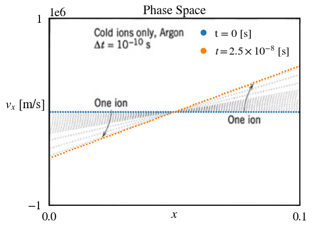
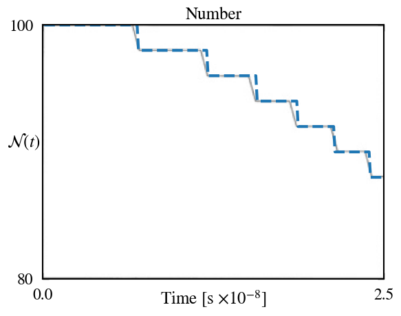
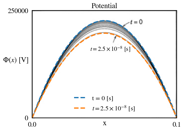
Results of the SALAMANDER simulation are directly compared to those reported in Lieberman and Lichtenberg (2005). The comparison of these results is accomplished by directly reproducing Figure 2.2 of Lieberman and Lichtenberg (2005) and plotting the SALAMANDER results directly on top of the published results, ensuring that the bounds of the axes presented in Lieberman and Lichtenberg (2005) are maintained. As seen in these figures, SALAMANDER is able to reproduce the results nearly exactly.
Running the Case
To run this input, use the following commands in your Terminal. The --allow-test-objects flag allows the use of custom SALAMANDER testing objects that are not used for "production" physics capability, but are useful for representing simple cases such as in this scenario.
  cd ~/projects/salamander/test/tests/benchmarking
  ../../../salamander-opt -i lieberman.i --allow-test-objects
  python plot_lieberman_results.py
References
- Michael A Lieberman and Allan J Lichtenberg.
Principles of plasma discharges and materials processing.
Wiley, 2nd edition, 2005.[BibTeX]