Code Verification with MOOSE
(a practical guide)
Contents
Theory vs. Practice
The theory will be mentioned, but putting the theory into practice will be the focus.
Idaho National Laboratory
www.inl.gov
Established in 2005, INL is the lead nuclear energy R&D laboratory for the Department of Energy
"Establish a world-class capability in the modeling and simulation of advanced energy systems..."
INL is the one of the largest employers in Idaho with 5,597 employees and 478 interns
In 2023 the INL budget was over $1.6 billion
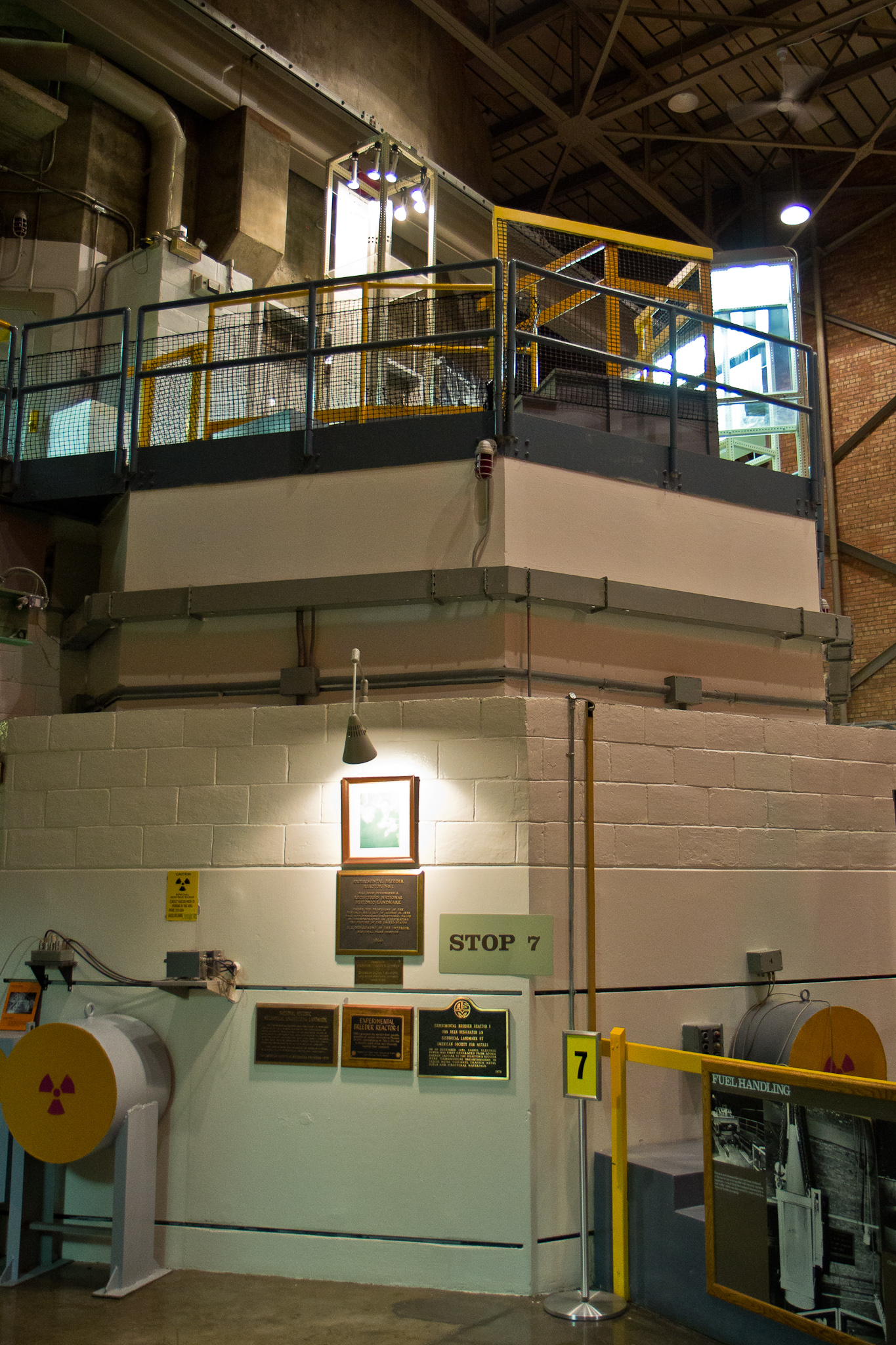
INL is the site where 52 nuclear reactors were designed and constructed, including the first reactor to generate usable amounts of electricity: Experimental Breeder Reactor I (EBR-1)
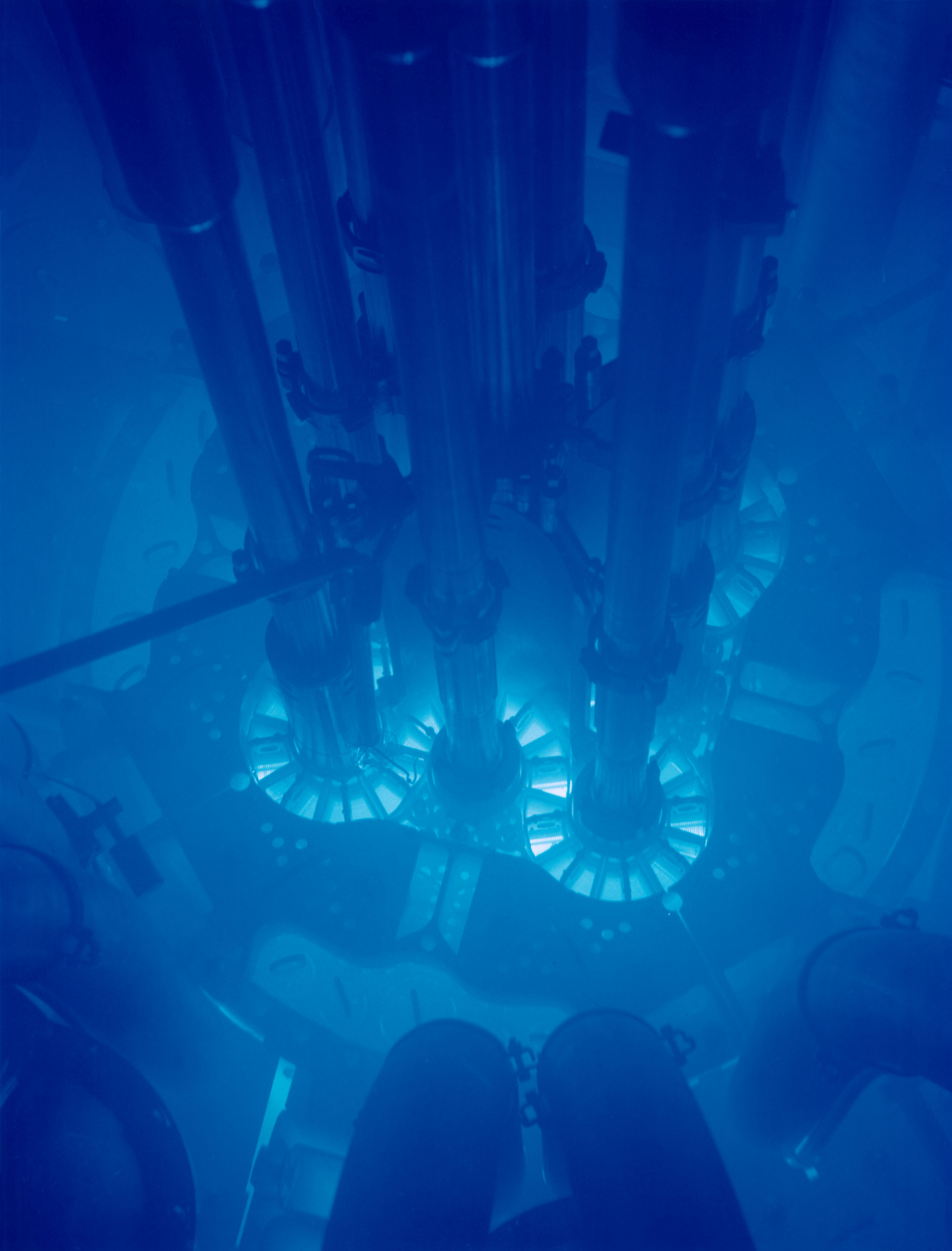
Advanced Test Reactor (ATR)
World's most powerful test reactor (250 MW thermal)
Constructed in 1967
Volume of 1.4 cubic meters, with 43 kg of uranium, and operates at 60C
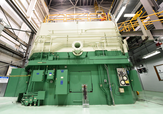
Transient Reactor Test Facility (TREAT)
TREAT is a test facility specifically designed to evaluate the response of fuels and materials to accident conditions
High-intensity (20 GW), short-duration (80 ms) neutron pulses for severe accident testing
National Reactor Innovation Center (NRIC)
NRIC is composed of two physical test beds to build prototypes of advanced nuclear reactors
DOME (Demonstration of Microreactor Experiments) in the historic EBR-II facility, a test bed site capable of hosting operational nuclear reactor concepts that produce less than 20MW thermal power.
LOTUS (Laboratory for Operation and Testing in the U.S.) in the historic Zero Power Physics Reactor (ZPPR) Cell, a test bed site capable of hosting operational nuclear reactor concepts that produce less than 500kW thermal power.
And an open-source online virtual test bed to demonstrate advanced reactors through modeling and simulation. More information about NRIC can be found at https://nric.inl.gov.
MOOSE Introduction
Multi-physics Object Oriented Simulation Environment
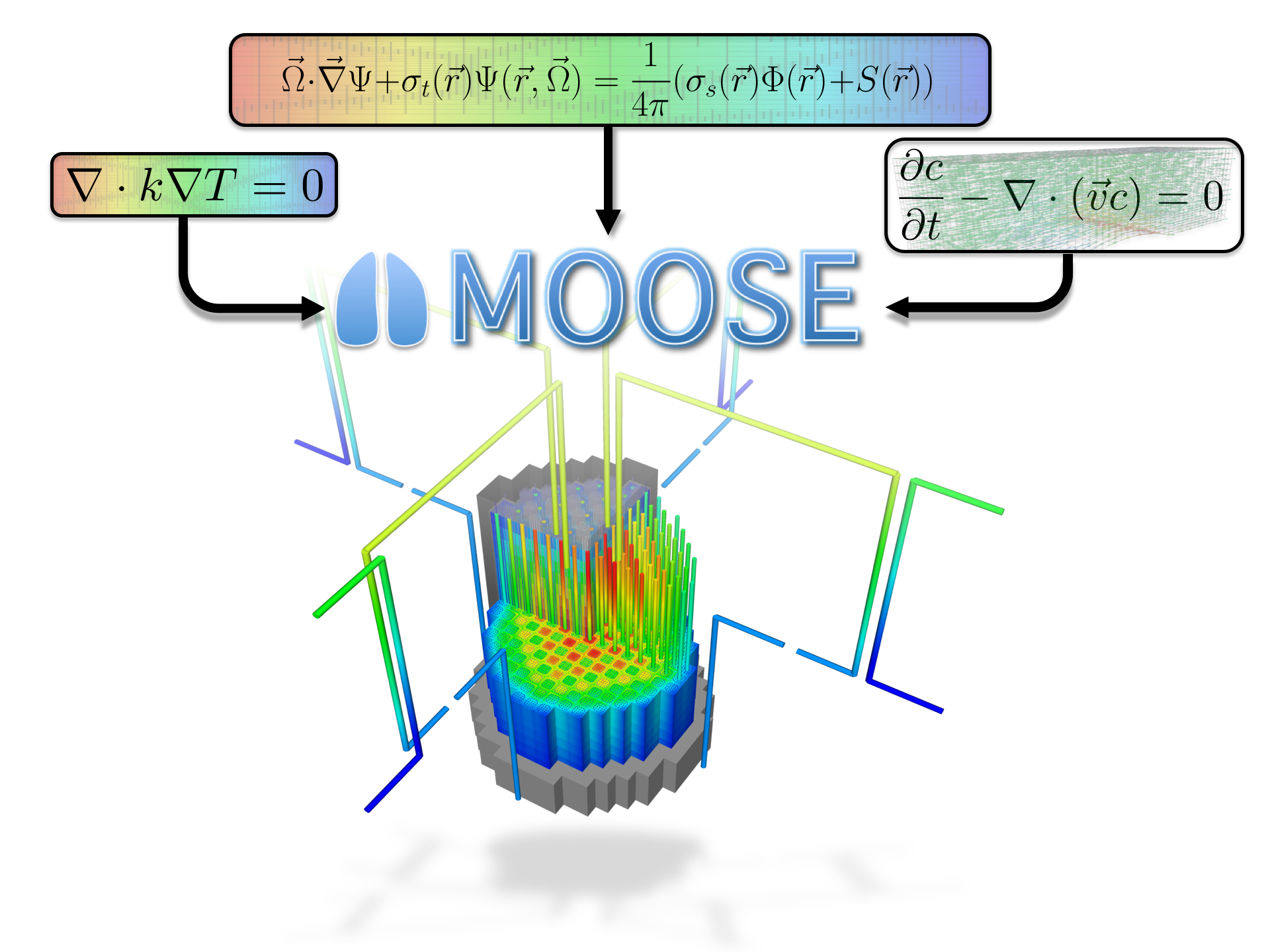
History and Purpose
Development started in 2008
Open-sourced in 2014
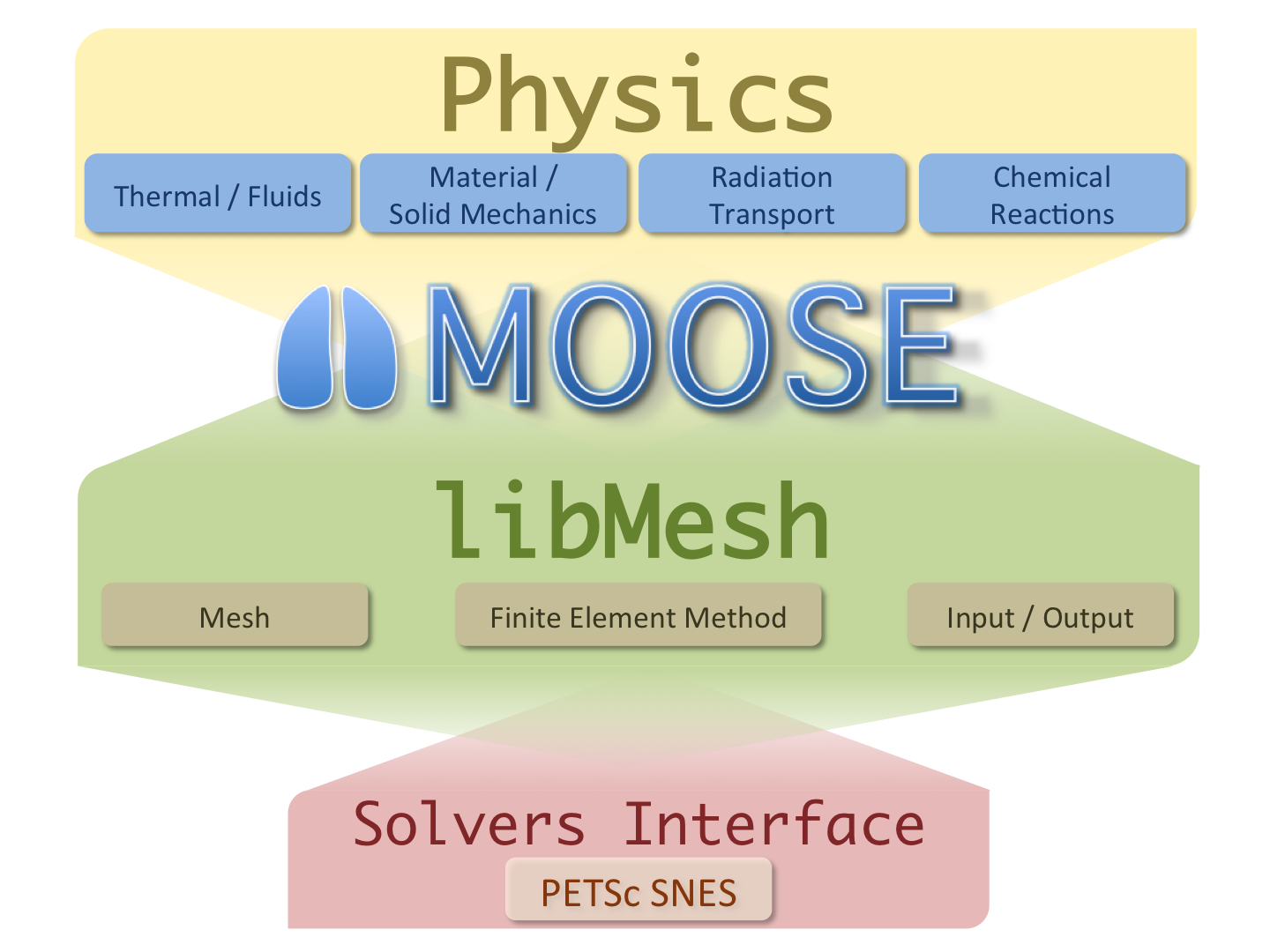
Designed to solve computational engineering problems and reduce the expense and time required to develop new applications by:
being easily extended and maintained
working efficiently on a few and many processors
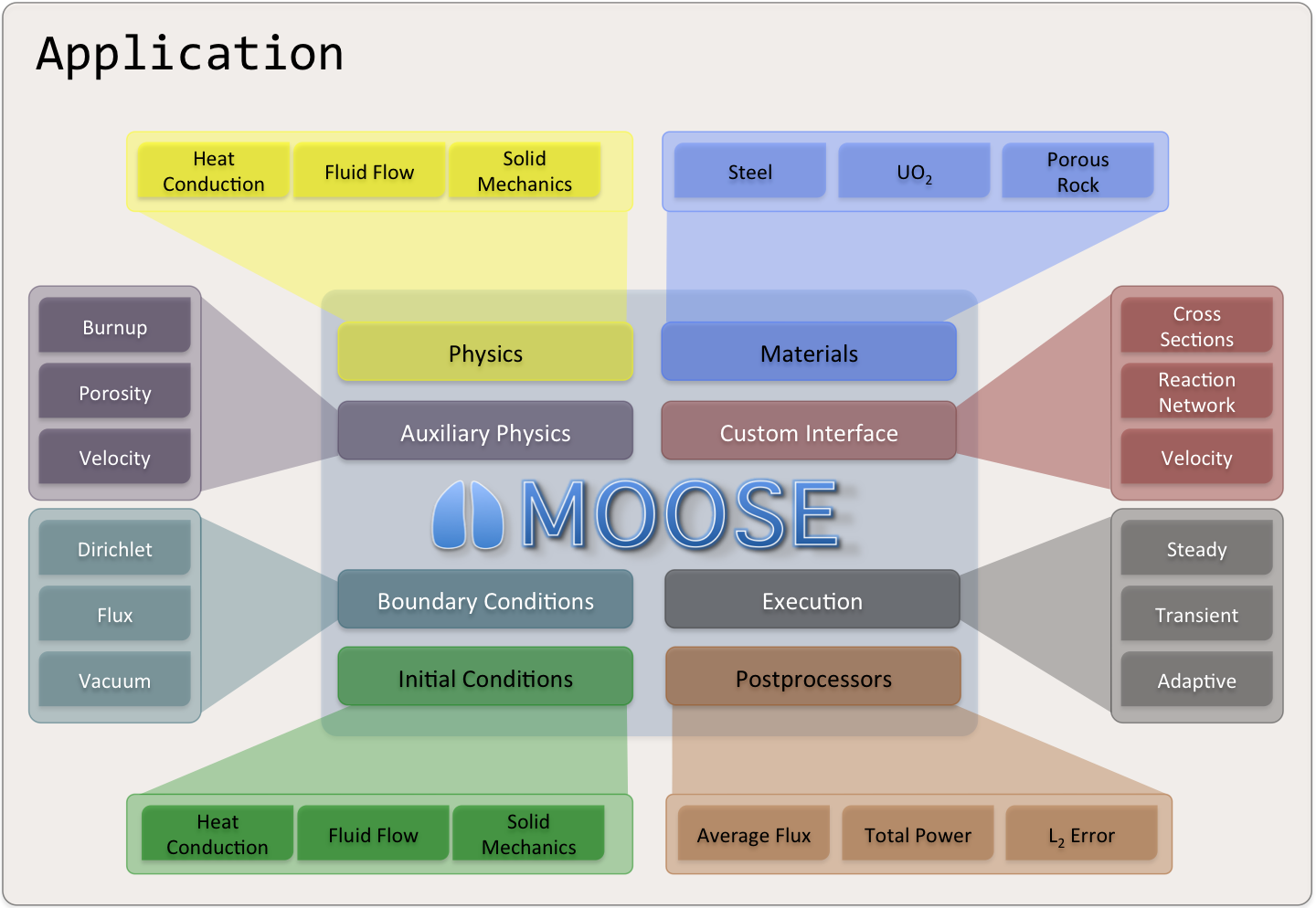
providing an object-oriented, extensible system for creating all aspects of a simulation tool
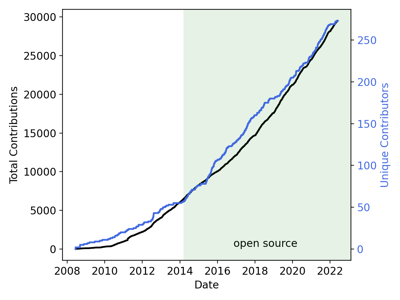
MOOSE By The Numbers
208 contributors
46,000 commits
5000 unique visitors per month
~6 new Discussion participants per week
1500 citations for the MOOSE papers
Most cited paper in Elsevier Software-X
More than 500 publications using MOOSE
30M tests per week
General Capabilities
Continuous and Discontinuous Galerkin FEM
Finite Volume
Supports fully coupled or segregated systems, fully implicit and explicit time integration
Automatic differentiation (AD)
Unstructured mesh with FEM shapes
Higher order geometry
Mesh adaptivity (refinement and coarsening)
Massively parallel (MPI and threads)
User code agnostic of dimension, parallelism, shape functions, etc.
Operating Systems:
macOS
Linux
Windows (WSL)
Object-oriented, pluggable system
Example Code
Software Quality
MOOSE follows an Nuclear Quality Assurance Level 1 (NQA-1) development process
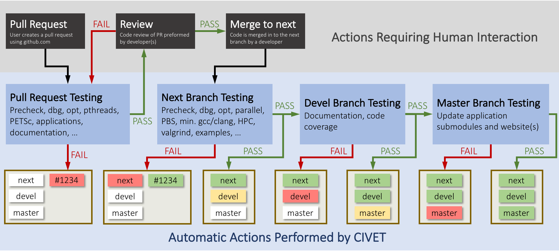
All commits undergo review using GitHub Pull Requests and must pass a set of application regression tests before they are available to our users
MOOSE includes a test suite and documentation system to allow for agile development while maintaining a NQA-1 process
Utilizes the Continuous Integration Environment for Verification, Enhancement, and Testing (CIVET)
External contributions are guided through the process by the team, and are very welcome!
Development Process
Community
https://github.com/idaholab/moose/discussions

License
LGPL 2.1
Does not limit what you can do with your application
Can license/sell your application as closed source
Modifications to the library itself (or the modules) are open source
New contributions are automatically LGPL 2.1
Verification
Theory
The term "verification" is rooted in software engineering practices and software quality standards.
The Institute of Electrical and Electronics Engineers (IEEE) defines verification as "The assurance that a product, service, or system meets the needs of the customer and other identified stakeholders. It often involves acceptance and suitability with external customers."
Practice
For our purposes, verification is the process of ensuring that the software is performing calculations as expected.
For a MOOSE-based application, ensure that the equations are solved correctly.
Process
The process of performing a verification study is simple in practice:
Perform simulation with a known solution and measure the error.
Refine the simulation (spatially or temporally) and repeat step 1.
If the error is reduced at the expected rate, then your simulation is numerically correct.
Convergence
Theory
Numerical integration and Finite Element Method (FEM) have known rates of convergence to the exact solution for decreasing time steps and element size.
Theory: Error
The error () shall be defined as the -norm of the difference between the finite element solution () and the known solution ().
where is the number of nodes for the simulation.
This is just one common measure of error, many others would work just as well.
Theory:
The time step size is easily computed as
where is time and is the time step number.
Theory: Element Size
There is no pre-defined measure of the element size.
Often alternatives for directly computing element information are used. For example, the square root of the number of degrees-of-freedom can be used as a measure of element size for 2D regular grids.
Practice: Error
MOOSE includes a number of error calculations, for Lagrange shape functions the -norm computed at the nodes is adequate.
[Postprocessors]
  [error]
    type = NodalL2Error
    variable = T
    function = T_exact
  []
[]
Practice:
[Postprocessors]
  [delta_t]
    type = TimestepSize
  []
[]
Practice: Element Size
[Postprocessors]
  [h]
    type = AverageElementSize
  []
[]
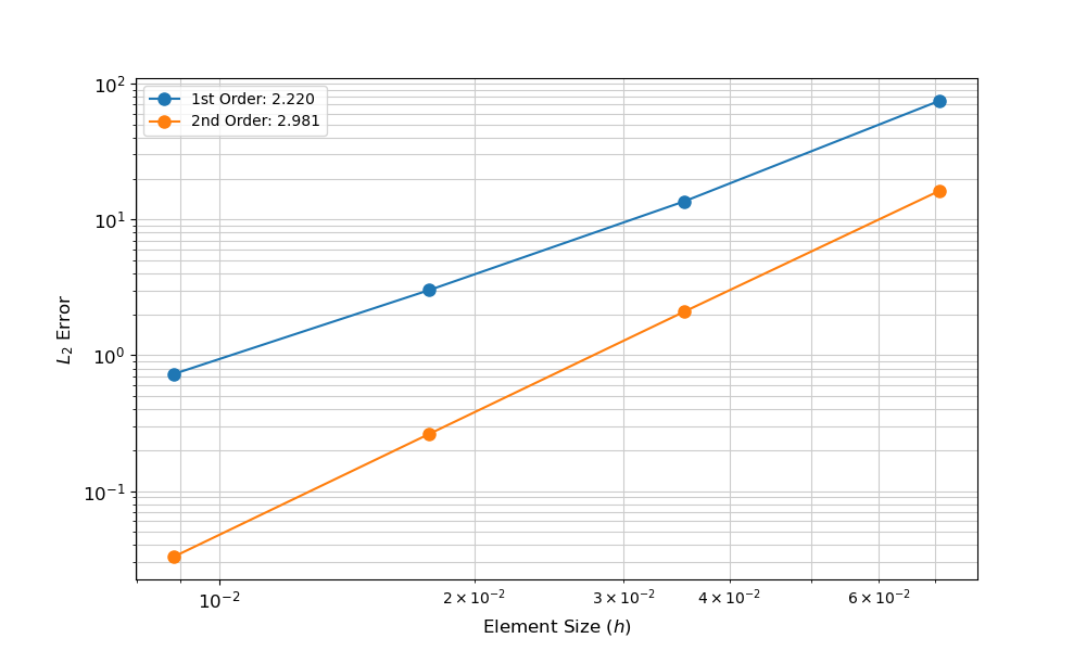
Practice: Spatial Convergence
Error decreases with decreasing element size, first-order elements converge with a slope of two and second-order three, when plotted on a log-log scale.
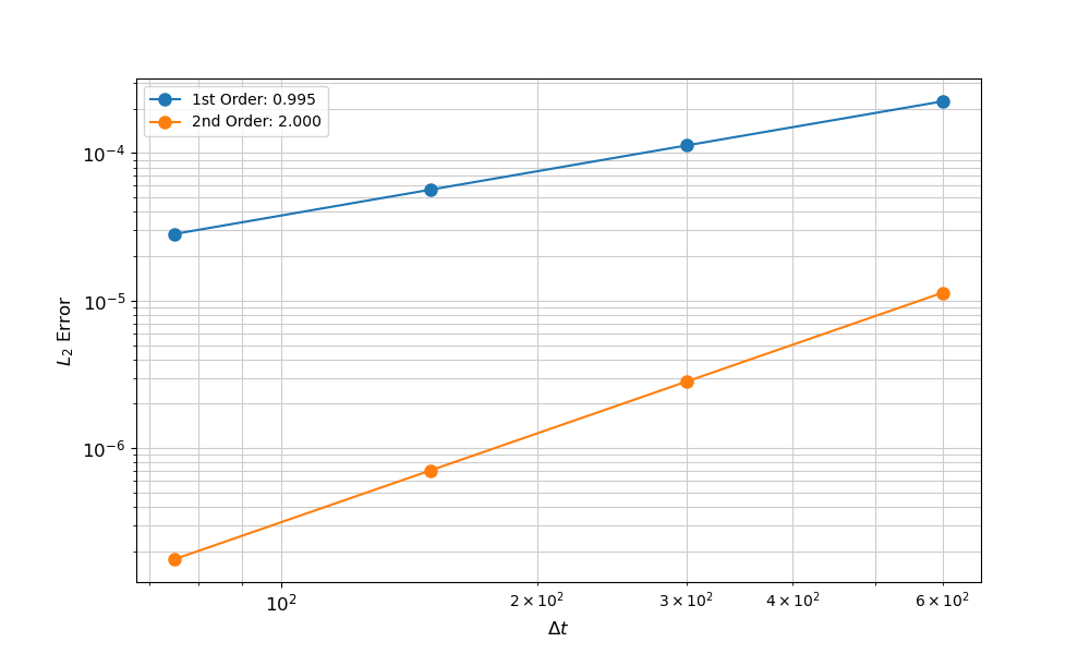
Practice: Temporal Convergence
Error decreases with decreasing time step size, with the slope equal to the order of the method when plotted on a log-log scale.
Heat Conduction
Theory: Heat Equation
where is temperature, is time, is the vector of spatial coordinates, is the density, is the specific heat capacity, is the thermal conductivity, is a heat source, and is the spatial domain.
Boundary conditions are defined on the boundary of the domain , the type and application of which will be discussed for the specific application of the heat equation throughout the tutorial.
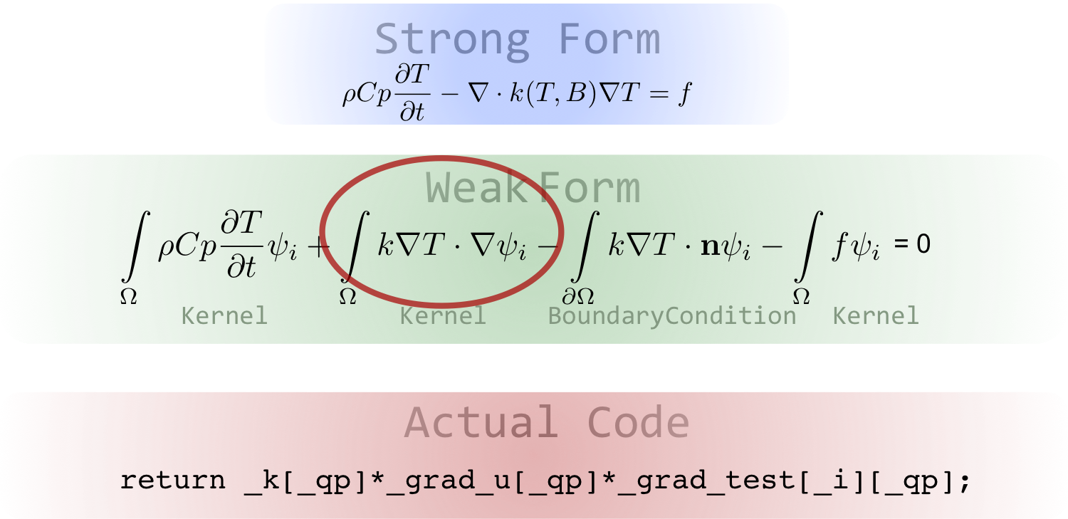
Theory: Weak Form
The weak form of the heat equation is necessary to utilize FEM, this is done by integrating over the domain () and multiplying by a set of test functions (). Performing these steps result in the weak form as follows, provided in inner-product notation.
where are the finite element test functions, is the finite element solution, and is the boundary outward facing normal vector. The boundary term is a result of using integration by parts and the divergence theorem.
This derivation also includes provisions for the application of Dirichlet boundary conditions, the details of which are not necessary for this tutorial.
Practice: Kernel Objects
In MOOSE, volume terms are represent by Kernel objects and added within the [Kernels] input block. For this problem the necessary objects exist within the heat transfer module.
HeatConductionTimeDerivative
[Kernels]
  [T_time]
    type = HeatConductionTimeDerivative
    variable = T
    density_name = 150
    specific_heat = 2000
  []
[]
Practice: Kernel Objects
HeatConduction
[Kernels]
  [T_cond]
    type = HeatConduction
    variable = T
    diffusion_coefficient = 0.01
  []
[]
HeatSouce
[Kernels]
  [T_source]
    type = HeatSource
    variable = T
    function = source
  []
[]
Practice: BoundaryCondition Objects
In MOOSE, boundary terms are represented by BoundaryCondition objects and added within the [BCs] input block. For this problem the necessary objects exist within the framework.
NeumannBC
[BCs]
  [top]
    type = NeumannBC
    boundary = top
    variable = T
    value = -5
  []
[]
Practice: BoundaryCondition Objects
The Dirichlet conditions, which prescribes a value on a boundary can also be utilized.
[BCs]
  [bottom]
    type = DirichletBC
    boundary = bottom
    variable = T
    value = 263.15
  []
[]
Analytic Solution
Summary
The best method for verifying a simulation is comparison with a known mathematical solution. For the heat equation, one such solution shall be considered to verify a model. The verification process shall be broken into four parts:
Define a problem, with a known exact solution.
Simulate the problem.
Compute the error between the known solution and simulation.
Perform convergence study.
Theory: Problem Statement
Incropera et al. (1996) presents a one-dimensional solution for the heat equation as:
where is the temperature, is the initial temperature, is time, is position, is the heat source, is thermal conductivity, and is the thermal diffusivity. Thermal diffusivity is defined as the ratio of thermal conductivity () to the product of density () and specific heat capacity (). The system is subjected to Neumann boundary conditions at the left boundary () and the natural boundary condition on the opposite boundary.
Practice: Simulation
Multiphysics Object Oriented Simulation Environment (MOOSE) operates using input files, as such, an input file shall be detailed that is capable of simulating this problem and its use demonstrated.
The location of this input file is arbitrary and it can be created and edited using any text editor program.
Domain
The domain of the problem is defined using the Mesh System using the [Mesh] block of the input file.
[Mesh]
  [gen]
    type = GeneratedMeshGenerator
    dim = 1
    xmax = 0.03
    nx = 200
  []
[]
Variable
There is a single unknown, temperature (), to compute. This unknown is declared using the Variables System in the [Variables] block and used the default configuration of a first-order Lagrange finite element variable.
[Variables]
  [T]
  []
[]
Kernels
The "volumetric" portions equation weak form are defined using the Kernel System in the [Kernels] block.
[Kernels]
  [T_time]
    type = HeatConductionTimeDerivative
    variable = T
    density_name = 7800
    specific_heat = 450
  []
  [T_cond]
    type = HeatConduction
    variable = T
    diffusion_coefficient = 80.2
  []
[]
Boundary Conditions
The boundary portions of the equation weak form are defined using the Boundary Condition System in the [BCs] block. At a Neumann condition is applied with a value of 7E5, by default is given the name of "left".
[BCs]
  [left]
    type = NeumannBC
    variable = T
    boundary = left
    value = 7e5
  []
[]
Execution
The problem is solved using Newton's method with a second-order backward difference formula (BDF2) with a timestep of 0.01 seconds up to a simulation time of one second. These settings are applied within the [Executioner] block using the Executioner System.
[Executioner]
  type = Transient
  scheme = bdf2
  solve_type = NEWTON
  dt = 0.01
  end_time = 1
[]
Output
The ExodusII and CSV format is enabled within the [Outputs] block using the Outputs System.
[Outputs]
  exodus = true
  csv = true
[]
Practice: Run
Executing the simulation is straightforward, simply execute the heat transfer module executable with the input file included using the "-i" option as follows.
~/projects/moose/modules/heat_transfer/heat_conduction-opt -i 1d_analytical.i
Practice: Compute Error
To compute the error the exact solution must be added, from which the error can be computed using the FEM solution.
Exact Solution
The known solution can be defined using the Function System in the Functions block.
[Functions]
  [T_exact]
    type = ParsedFunction
    symbol_names = 'k    rho  cp  T0  qs'
    symbol_values = '80.2 7800 450 300 7e5'
    expression = 'T0 + qs/k*(2*sqrt(k/(rho*cp)*t/pi)*exp(-x^2/(4*k/(rho*cp)*(t+1e-50))) - x*(1-erf(x/(2*sqrt(k/(rho*cp)*(t+1e-50))))))'
  []
[]
The "vars" and "vals" have a one-to-one relationship, e.g., . If defined in this manner then the names in "vars" can be used in the definition of the equation in the "value" parameter.
Error
The -norm of the difference between the computed and exact solution can be computed using the NodalL2Error object. This is created within the [Postprocessors] block along with the average element size.
[Postprocessors]
  [error]
    type = NodalL2Error
    variable = T
    function = T_exact
  []
  [h]
    type = AverageElementSize
  []
[]
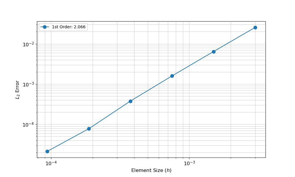
Practice: Convergence Rate
MOOSE includes a python package—the mms package—for performing convergence studies, as such shall be used here.
Spatial Convergence
To perform a spatial convergence the input file create needs to be executed with decreasing element size, which in MOOSE can be done by adding the Mesh/uniform_refine=x option to the command line with "x" being an integer representing the number of refinements to perform.
import mms
df = mms.run_spatial('1d_analytical.i', 6, 'Mesh/gen/nx=10', console=False)
fig = mms.ConvergencePlot(xlabel='Element Size ($h$)', ylabel='$L_2$ Error')
fig.plot(df, label='1st Order', marker='o', markersize=8)
fig.save('1d_analytical_spatial.png')
Temporal
The temporal convergence study is nearly identical to the spatial. For a temporal study, the time step is reduced.
import mms
df = mms.run_temporal('1d_analytical.i', 6, dt=0.5, console=False)
fig = mms.ConvergencePlot(xlabel='$\Delta t$', ylabel='$L_2$ Error')
fig.plot(df, label='2nd Order (Backward Difference)', marker='o', markersize=8)
fig.save('1d_analytical_temporal.png')
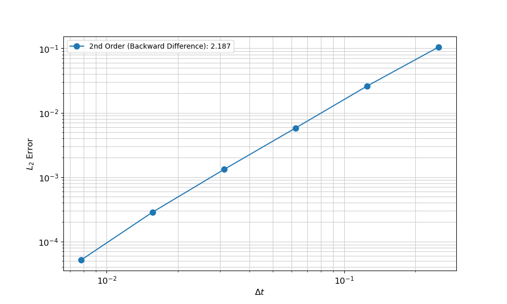
Practice: Closing Remark
The resulting convergence data indicate that the simulation is converging to the known solution at the correct rate for linear shape functions and second-order time integration. Thus, it can be stated that this simulation is verified.
Method of Manufactured Solution
Summary
In practice an exact solution is not known, since there would be no reason to perform a simulation if the answer is known.
It is possible to "manufacture" a solution using the Method of Manufactured Solutions (MMS).
The two-dimensional heat equation will be used to simulate a physical system and used as basis for spatial and temporal convergence study using the MMS.
Theory: Method of Manufactured Solution
The MMS can be summarized into three basic steps:
Assume a solution for the partial differential equation (PDE) of interest:
Apply assumed solution to compute a residual function. For example,
Add the negative of the computed function and perform the desired convergence study. For example, the PDE above becomes:
This PDE has a known solution, , that can be used to compute the error and perform a convergence study.
Assumed Solution
The form of the solution is arbitrary, but certain characteristics are desirable to eliminate an unnecessary accumulation of error.
For a spatial study, the solution should not be exactly represented by the shape functions and should be exactly represented by the numerical integration scheme.
For a temporal study, the solution should be exactly represent by the shape functions and should not be exactly represented by the numerical integration scheme.
Theory: Problem Statement
The two-dimensional heat equation shall be used to simulate a cross section of snow subjected to radiative cooling at the surface and internal heating due to solar absorption.
The domain is defined as and .
A heat source, , is applied as an approximation of internal heating due to solar absorption. The source is raised from zero to a maximum of 650 back to zero during a 9 hours (32400 sec.) period following a sine function. The duration is an approximation of the daylight hours in Idaho Falls, Idaho in December.
The left side of the domain is shaded and the right is subjected to the maximum source, again defined using a sine function.
The top surface () is subjected to a Neumann boundary condition, , which approximates the radiative cooling of the snow surface.
Theory: Material Properties
| Variable | Value | Units |
|---|---|---|
| 263.15 | ||
| 0.01 | ||
| 150 | ||
| 2000 | ||
| 40 | ||
| -5 | ||
| 263.15 |
Practice: Simulation
The heat transfer module is capable of performing this simulation, thus only an input file is needed to simulate this problem.
Domain
The problem requires a two-dimensional rectangular domain, which can be defined using the Mesh System as defined in the [Mesh] block of the input.
[Mesh]
  [gen]
    type = GeneratedMeshGenerator
    dim = 2
    ymax = 0
    ymin = -0.2
    nx = 20
    ny = 4
  []
[]
Variable
There is a single unknown, temperature (), to compute. This unknown is declared using the Variables System in the [Variables] block and used the default configuration of a first-order Lagrange finite element variable.
[Variables]
  [T]
  []
[]
Initial Conduction
The initial condition () is applied using the Initial Condition System in the [ICs] block. In this case a constant value throughout the domain is provided.
[ICs]
  [T_O]
    type = ConstantIC
    variable = T
    value = 263.15
  []
[]
Heat Source
The volumetric heat source, , is defined using the Function System using the [Functions] block. The variables "x", "y", "z", and "t" are always available and represent the corresponding spatial location and time.
[Functions]
  [source]
    type = ParsedFunction
    symbol_names = 'hours shortwave kappa'
    symbol_values = '9     650      40'
    expression = 'shortwave*sin(0.5*x*pi)*exp(kappa*y)*sin(1/(hours*3600)*pi*t)'
  []
[]
Kernels
The "volumetric" portions of the weak form of the equation are defined using the Kernel System in the [Kernels] block, for this example this can be done with the use of three Kernel objects as follows.
[Kernels]
  [T_time]
    type = HeatConductionTimeDerivative
    variable = T
    density_name = 150
    specific_heat = 2000
  []
  [T_cond]
    type = HeatConduction
    variable = T
    diffusion_coefficient = 0.01
  []
  [T_source]
    type = HeatSource
    variable = T
    function = source
  []
[]
Boundary Conditions
The boundary portions of the equation weak form are defined using the Boundary Condition System in the [BCs] block. At top of the domain () a Neumann condition is applied with a constant outward flux. On the button of the domain () a constant temperature is defined. The remain boundaries are "insulated", which is known as the natural boundary condition.
[BCs]
  [top]
    type = NeumannBC
    boundary = top
    variable = T
    value = -5
  []
  [bottom]
    type = DirichletBC
    boundary = bottom
    variable = T
    value = 263.15
  []
[]
Execution
The problem is solved using Newton's method with a first-order backward Euler method with a timestep of 600 seconds (10 min.) up to a simulation time of nine hours. These settings are applied within the [Executioner] block using the Executioner System.
[Executioner]
  type = Transient
  solve_type = 'NEWTON'
  dt = 600 # 10 min
  end_time = 32400 # 9 hour
[]
Output
The ExodusII and CSV format is enabled within the [Outputs] block using the Outputs System.
[Outputs]
  exodus = true
[]
Practice: Run
Executing the simulation is straightforward, simply execute the heat transfer module executable with the input file included using the "-i" option as follows.
~/projects/moose/modules/heat_transfer/heat_conduction-opt -i 2d_main.i
Practice: Convergence Rate
MOOSE includes a python package—the mms package—for performing convergence studies, as such shall be used here.
Spatial Convergence: Assumed Solution
Assume a solution to the desired PDE.
The solution cannot be exactly represented by the first-order shape functions.
The first-order time integration can capture the time portion of the equation exactly, thus does not result in temporal error accumulation.
Spatial Convergence: Forcing Function
The mms package can compute the necessary forcing function and output the input file syntax for both the forcing function and the assumed solution.
import mms
fs, ss = mms.evaluate(('rho * cp * diff(u,t) - div(k*grad(u)) - '
                      'shortwave*sin(0.5*x*pi)*exp(kappa*y)*sin(1/(hours*3600)*pi*t)'),
                      't*sin(pi*x)*sin(5*pi*y)',
                      scalars=['rho', 'cp', 'k', 'kappa', 'shortwave', 'hours'])
mms.print_hit(fs, 'mms_force')
mms.print_hit(ss, 'mms_exact')
Executing this script, assuming a name of spatial_function.py results in the following output.
$ python spatial_function.py
[mms_force]
  type = ParsedFunction
  value = 'cp*rho*sin(x*pi)*sin(5*y*pi) + 26*pi^2*k*t*sin(x*pi)*sin(5*y*pi) - shortwave*exp(y*kappa)*sin((1/2)*x*pi)*sin((1/3600)*pi*t/hours)'
  vars = 'hours rho shortwave k cp kappa'
  vals = '1.0 1.0 1.0 1.0 1.0 1.0'
[]
[mms_exact]
  type = ParsedFunction
  value = 't*sin(x*pi)*sin(5*y*pi)'
[]
Spatial Convergence: Input
MOOSE allows for multiple input files to be supplied to an executable, when this is done the inputs are combined into a single file that comprises the union of the two files.
The additional blocks required to perform the spatial convergence study and be created in an independent file.
Forcing and Solution Functions
The forcing function and exact solution are added using a parsed function, in similar to the existing functions withing the simulation.
[Functions]
  [mms_force]
    type = ParsedFunction
    expression = 'cp*rho*sin(x*pi)*sin(5*y*pi) + 26*pi^2*k*t*sin(x*pi)*sin(5*y*pi) - shortwave*exp(y*kappa)*sin((1/2)*x*pi)*sin((1/3600)*pi*t/hours)'
    symbol_names = 'rho cp   k     kappa shortwave hours'
    symbol_values = '150 2000 0.01  40    650       9'
  []
  [mms_exact]
    type = ParsedFunction
    expression = 't*sin(pi*x)*sin(5*pi*y)'
  []
[]
Forcing Function as Heat Source
The forcing function is applied to the simulation by adding another heat source Kernel object.
[Kernels]
  [mms]
    type = HeatSource
    variable = T
    function = mms_force
  []
[]
Error and Element Size
To perform the study the error and element size are required, these are added as Postprocessors block.
[Postprocessors]
  [error]
    type = ElementL2Error
    variable = T
    function = mms_exact
  []
  [h]
    type = AverageElementSize
  []
[]
Output
CSV output also needs to be added, which is added as expected.
[Outputs]
  csv = true
[]
Boundary and Initial Conditions
The initial and boundary conditions for the simulation do not satisfy the assumed solution. The easiest approach to remedy this is to use the assumed solution to set both the initial condition and boundary conditions.
[BCs]
  active = 'mms'
  [mms]
    type = FunctionDirichletBC
    variable = T
    boundary = 'left right top bottom'
    function = mms_exact
  []
[]
[ICs]
  active = 'mms'
  [mms]
    type = FunctionIC
    variable = T
    function = mms_exact
  []
[]
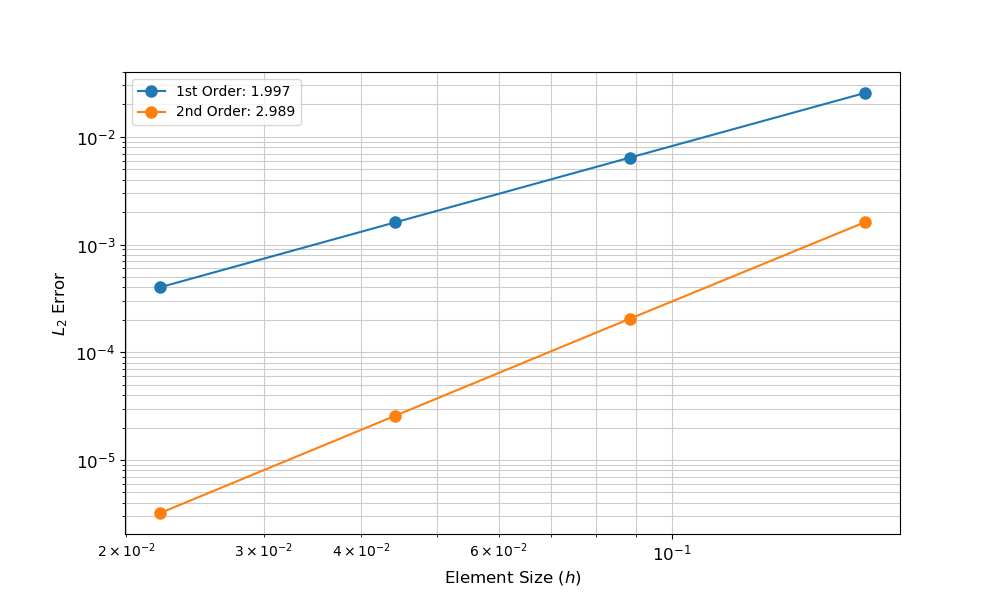
Spatial Convergence: Run
The mms package can be used to perform the convergence study. In this case, both a first and second-order shape functions are considered.
import mms

df1 = mms.run_spatial(['2d_main.i', '2d_mms_spatial.i'], 4, console=False)
df2 = mms.run_spatial(['2d_main.i', '2d_mms_spatial.i'], 4, 'Mesh/second_order=true', 'Variables/T/order=SECOND', console=False)

fig = mms.ConvergencePlot(xlabel='Element Size ($h$)', ylabel='$L_2$ Error')
fig.plot(df1, label='1st Order', marker='o', markersize=8)
fig.plot(df2, label='2nd Order', marker='o', markersize=8)
fig.save('2d_mms_spatial.png')
Temporal Convergence: Assumed Solution
Assume a solution to the desired PDE.
The solution can be exactly represented by the first-order shape functions, thus does not result in spatial error accumulation.
The first-order time integration cannot capture the time portion of the equation exactly.
Temporal Convergence: Forcing Function
The mms package can compute the necessary forcing function and output the input file syntax for both the forcing function and the assumed solution.
import mms
fs, ss = mms.evaluate(('rho * cp * diff(u,t) - div(k*grad(u)) - '
                      'shortwave*sin(0.5*x*pi)*exp(kappa*y)*sin(1/(hours*3600)*pi*t)'),
                      'x*y*exp(-1/32400*t)',
                      scalars=['rho', 'cp', 'k', 'kappa', 'shortwave', 'hours'])
mms.print_hit(fs, 'mms_force')
mms.print_hit(ss, 'mms_exact')
Executing this script, assuming a name of temporal_function.py results in the following output.
$ python temporal_function.py
[mms_force]
  type = ParsedFunction
  value = '-3.08641975308642e-5*x*y*cp*rho*exp(-3.08641975308642e-5*t) - shortwave*exp(y*kappa)*sin((1/2)*x*pi)*sin((1/3600)*pi*t/hours)'
  vars = 'kappa rho shortwave cp hours'
  vals = '1.0 1.0 1.0 1.0 1.0'
[]
[mms_exact]
  type = ParsedFunction
  value = 'x*y*exp(-3.08641975308642e-5*t)'
[]
Temporal Convergence: Input
A third input is created. The content follows the input to the spatial counter part and as such is included completely below.
[ICs]
  active = 'mms'
  [mms]
    type = FunctionIC
    variable = T
    function = mms_exact
  []
[]

[BCs]
  active = 'mms'
  [mms]
    type = FunctionDirichletBC
    variable = T
    boundary = 'left right top bottom'
    function = mms_exact
  []
[]

[Kernels]
  [mms]
    type = HeatSource
    variable = T
    function = mms_force
  []
[]

[Functions]
  [mms_force]
    type = ParsedFunction
    expression = '-3.08641975308642e-5*x*y*cp*rho*exp(-3.08641975308642e-5*t) - shortwave*exp(y*kappa)*sin((1/2)*x*pi)*sin((1/3600)*pi*t/hours)'
    symbol_names = 'rho cp   k     kappa shortwave hours'
    symbol_values = '150 2000 0.01  40    650       9'
  []
  [mms_exact]
    type = ParsedFunction
    expression = 'x*y*exp(-3.08641975308642e-5*t)'
  []
[]

[Outputs]
  csv = true
[]

[Postprocessors]
  [error]
    type = ElementL2Error
    variable = T
    function = mms_exact
  []
  [delta_t]
    type = TimestepSize
  []
[]
Temporal Convergence: Run
The mms package can be used to perform the convergence study. In this case, both first and second-order shape functions are considered.
import mms

df1 = mms.run_temporal(['2d_main.i', '2d_mms_temporal.i'], 4, dt=1200, mpi=4, console=False)
df2 = mms.run_temporal(['2d_main.i', '2d_mms_temporal.i'], 4, 'Executioner/scheme=bdf2', dt=1200, mpi=4, console=False)
fig = mms.ConvergencePlot(xlabel='$\Delta t$', ylabel='$L_2$ Error')
fig.plot(df1, label='1st Order', marker='o', markersize=8)
fig.plot(df2, label='2nd Order', marker='o', markersize=8)
fig.save('2d_mms_temporal.png')
References
- Frank P Incropera, David P DeWitt, Theodore L Bergman, Adrienne S Lavine, and others. Fundamentals of heat and mass transfer. Volume 6. Wiley New York, 1996.