MOOSE MultiApps
Introduction
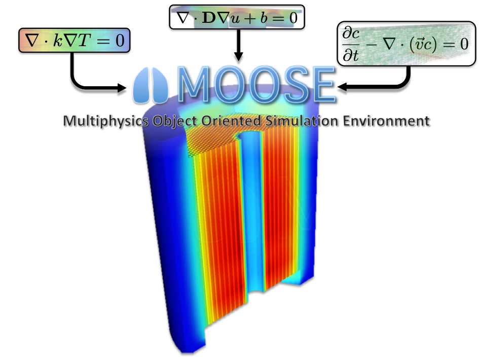
MOOSE
Started in May of 2008
A framework enabling rapid development of new simulation tools
NQA-1 Compliant
Application development focuses on implementing physics (PDEs) rather than numerical implementation issues
Seamlessly couples native (MOOSE) applications using MOOSE MultiApps and Transfers
Efficiently couples non-native codes using MOOSE-Wrapped Apps
Open Sourced February 12, 2014
Coupling
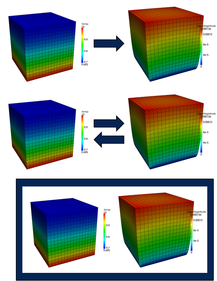
Loosely-Coupled
Each physics solved with a separate linear/nonlinear solve.
Data exchange once per timestep (typically)
Tightly-Coupled / Picard
Each physics solved with a separate linear/nonlinear solve.
Data is exchanged and physics re-solved until “convergence”
Fully-Coupled
All physics solved for in one linear/nonlinear solve
MultiApps and Transfers
MOOSE was originally created to solve fully-coupled systems of PDEs.
Not all systems need to be / are fully coupled:
Multiscale
Systems with multiple timescales.
Coupling to external codes.
To MOOSE these situations look like loosely-coupled systems of fully-coupled equations.
The MultiApp system allows multiple MOOSE (or external) applications to run simultaneously in parallel.
A single MultiApp might represent thousands of individual solves.
The Transfer system in MOOSE is designed to push and pull fields and data to and from MultiApps.
MultiApps
MOOSE-based solves can be nested to achieve multiscale Multiphysics simulations
Macroscale simulations can be coupled to embedded microstructure simulations
Arbitrary levels of solves
Each solve is spread out in parallel to make the most efficient use of computing resources
Efficiently ties together multiple team’s codes
MOOSE-wrapped, external applications can exist anywhere in this hierarchy
Apps do NOT know they are running within the MultiApp hierarchy!

Transfers
Transfers allow you to move data between MultiApps
Three main catergories of Transfers exist in MOOSE:
Field Mapping
L2 Projection, Interpolation, Evaluation
“Postprocessed” Spatial Data
e.g.: Layered Integrals and Averages, Assembly Averaged Data, etc.
Scalar Transfer
Postprocessor values (Integrals, Averages, Point Evaluations, etc.)
Can be transferred as a scalar or interpolated into a field.
Useful for multi-scale
All Transfers are agnostic of dimension (if it makes sense!)
When transferring to or from a MultiApp a single Transfer will actually transfer to or from ALL sub-apps in that Multi-App simultaneously.
Step01 MultiApps
Input File Syntax
MultiApp objects are declared in the [MultiApps] block and require a type just like many other blocks.
The app_type is required and is the name of the MooseApp derived app that is going to be executed. Generally, this is the name of the application being executed, therefore if this parameter is omitted it will default as such. However this system is designed for running other applications that are compiled or linked into the current app.
A MultiApp can be executed at any point during the parent app solve by setting the execute_on parameter. The positions parameters is a list of 3D coordinate pairs describing the offset of the sub-application(s) into the physical space of the parent application.
[MultiApps]
  [sub_app]
    type = TransientMultiApp
    app_type = MooseTestApp
    input_files = 'dt_from_parent_sub.i'
    positions = '0   0   0
                 0.5 0.5 0
                 0.6 0.6 0
                 0.7 0.7 0'
  []
[]
Positions
The positions parameter is a coordinate offset from the parent app domain to the sub-app domain, as illustrated below. The parameter requires the positions to be provided as a set of coordinates for each sub-app.
The number of coordinate sets determines the actual number of sub-applications created. If there is a large number of positions a file can be provided instead using the positions_file parameter. For alternative ways to specify positions, notably dynamically during the simulation, use the [Positions] block.
The coordinates are a vector that is being added to the coordinates of the sub-app's domain to put that domain in a specific location within the parent app domain.
If the sub-app's domain starts at it is easy to think of moving that point around using
positions.For sub-apps on completely different scales,
positionsis the point in the parent app domain where that app is located.
MultiApp Position
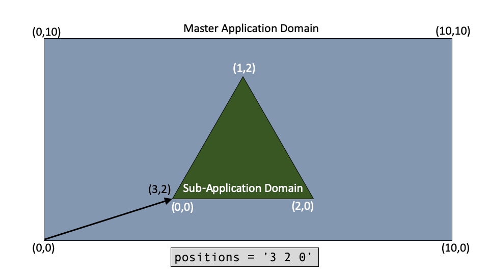
Figure 1: Example of MultiApp object position.
Parallel Execution
The MultiApp system is designed for efficient parallel execution of hierarchical problems. The parent application utilizes all processors. Within each MultiApp, all of the processors are split among the sub-apps. If there are more sub-apps than processors, each processor will solve for multiple sub-apps. All sub-apps of a given MultiApp are run simultaneously in parallel. Multiple MultiApps will be executed one after another.
Dynamically Loading Multiapps
If building with dynamic libraries (the default) other applications can be loaded without adding them to your Makefile and registering them. Simply set the proper type in your input file (e.g. AnimalApp) and MOOSE will attempt to find the other library dynamically.
The path (relative preferred) can be set in your input file using the parameter
library_path; this path needs to point to thelibfolder within an application directory.The
MOOSE_LIBRARY_PATHmay also be set to include paths for MOOSE to search.
Each application must be compiled separately since the main application Makefile does not have knowledge of any sub-app application dependencies.
Basic MultiApp
To get started, let's consider a simple system with two apps as shown on the right.
For now: no Transfers so no coupling
Each application will march forward in time together, solve, and output

01_parent.i
[Mesh]
  type = GeneratedMesh
  dim = 2
  nx = 10
  ny = 10
[]

[Variables]
  [u]
  []
[]

[Kernels]
  [diff]
    type = Diffusion
    variable = u
  []
  [force]
    type = BodyForce
    variable = u
    value = 1.
  []
  [td]
    type = TimeDerivative
    variable = u
  []
[]

[BCs]
  [left]
    type = DirichletBC
    variable = u
    boundary = left
    value = 0
  []
  [right]
    type = DirichletBC
    variable = u
    boundary = right
    value = 0
  []
[]

[Executioner]
  type = Transient
  end_time = 2
  dt = 1.

  solve_type = 'PJFNK'

  petsc_options_iname = '-pc_type -pc_hypre_type'
  petsc_options_value = 'hypre boomeramg'
[]

[Outputs]
  exodus = true
[]

[MultiApps]
  [sub_app]
    type = TransientMultiApp
    positions = '0 0 0'
    input_files = '01_sub.i'
  []
[]
01_sub.i
[Mesh]
  type = GeneratedMesh
  dim = 2
  nx = 10
  ny = 10
[]

[Variables]
  [v]
  []
[]

[Kernels]
  [diff]
    type = Diffusion
    variable = v
  []
  [td]
    type = TimeDerivative
    variable = v
  []
[]

[BCs]
  [left]
    type = DirichletBC
    variable = v
    boundary = left
    value = 0
  []
  [right]
    type = DirichletBC
    variable = v
    boundary = right
    value = 1
  []
[]

[Executioner]
  type = Transient
  end_time = 2
  dt = 1

  solve_type = 'PJFNK'

  petsc_options_iname = '-pc_type -pc_hypre_type'
  petsc_options_value = 'hypre boomeramg'
[]

[Outputs]
  exodus = true
[]
Note how the sub-app input file doesn't even "know" it's being run within a MultiApp hierarchy!
Run 01_parent.i
Look at the order of execution
Inspect outputs
Modify
execute_onto see what happens
Sub-App Constraining dt
By default the MultiApp system will "negotiate" a timestep dt that makes sense for the entire hierarchy: it will choose the smallest dt that any app is currently requesting
Let's modify the sub-app to have a smaller timestep and see what happens
02_sub_sublimit.i
[Mesh]
  type = GeneratedMesh
  dim = 2
  nx = 10
  ny = 10
[]

[Variables]
  [v]
  []
[]

[Kernels]
  [diff]
    type = Diffusion
    variable = v
  []
  [td]
    type = TimeDerivative
    variable = v
  []
[]

[BCs]
  [left]
    type = DirichletBC
    variable = v
    boundary = left
    value = 0
  []
  [right]
    type = DirichletBC
    variable = v
    boundary = right
    value = 1
  []
[]

[Executioner]
  type = Transient
  end_time = 2
  dt = 0.2

  solve_type = 'PJFNK'

  petsc_options_iname = '-pc_type -pc_hypre_type'
  petsc_options_value = 'hypre boomeramg'
[]

[Outputs]
  exodus = true
[]
Run 02_parent_sublimit.i
Note the timestep being used by each app

Subcycling
Forcing all apps to take the same timestep size is very limiting.
Often better to allow the sub-app to take smaller timesteps. For instance: if the sub-app is a CFD calculation, the timestep size may be limited by numerical criteria or material properties (CFL conditions, etc.).
To allow this: set sub_cycling=true in the MultiApp block:
03_parent_subcycle.i
[MultiApps]
  [sub_app]
    type = TransientMultiApp
    positions = '0 0 0'
    input_files = '03_sub_subcycle.i'
    sub_cycling = true
    #    output_sub_cycles = true
  []
[]
Run 03_parent_subcycle.i
Note the timestep size used by each solve
The sub-app will take however many timesteps are needed to reach the parent app's time
What happens if the timesteps aren't even?
By default the intermediate steps are NOT output - only the final solution once the sub-app reaches the parent app's time. To enable outputting all steps solved by the sub-app turn on output_subcycles in the MultiApp block.
Multiple Sub-Apps
Now for a more complicated scenario: multiple sub-apps within the same MultiApp.
This is achieved by giving each sub-app a position where that sub-app's domain lies within the parent app's domain.
There are three ways to provide positions:
positions: Space separated x,y,z triplets for the position of each sub-apppositions_file: A filename that includes x,y,z triplets (one per line)in the
[Positions]block, from the mesh, from various files, etc
The positions_file option is useful if you have MANY sub-apps (for instance: tens of thousands!).
There are two options for specifying input files for the positions:
A single input file: every sub-app will utilize the same input file
One input file for each position: every sub-app utilizes a separate input file
Multiple Sub-App Hierarchy
04_parent_multiple.i
[MultiApps]
  [sub_app]
    type = TransientMultiApp
    positions = '0 0 0  1 0 0  2 0 0'
    #    positions_file = 04_positions.txt
    input_files = '04_sub1_multiple.i'
    #    input_files = '04_sub1_multiple.i  04_sub2_multiple.i 04_sub3_multiple.i'
    #    output_in_position = true
  []
[]

Run 04_parent_multiple.i
Note how there are now three solves when the MultiApp executes
Note the names of the output files
Try using the
positions_fileinsteadTry using different input files for each position
Since sub-apps are "offset" into the parent app's domain - the output_in_position option can be used to make the output mesh from each sub-app reflect its "true" position within the simulation. Turn it on and re-visualize the sub-app solutions
Parallelism
When operating in parallel the MultiApps and sub-apps can be spread across the available processors (MPI-ranks) for faster execution.
The parent app always runs on the full amount of processors. For this reason, it's often advantageous to make the parent app the largest, most difficult solve.
Each MultiApp executes one-at-a-time (will be clear momentarily). The sub-apps within a MultiApp are all executed simultaneously (if possible).
To achieve this, the available processors are evenly split among the sub-apps within each MultiApp, as shown on the right.

Run 05_parent_parallel.i
Try 1, 3, 6 MPI procs
Note the MultiApp Execution time
Try with
--keep-cout
Note: to execute in parallel use:
mpiexec -n # ./theapp -i input.i
where you replace # with the number of MPI processes to start. If you are on a cluster you will need to consult your cluster's documentation for instructions.
Multiple MultiApps
As discussed before, MultiApps can represent an arbitrary tree of solves. Often it's the case that one solve may have more than one MultiApp in it. For instance, a nuclear reactor simulation may need to have solves underneath it for what's happening to the fuel and, separately, what's happening to the fluid.
In parallel, the MultiApps each receive the full amount of processors available from the parent app. The processors are then split between the sub-apps. This means that the MultiApps will execute "in-turn" in parallel - one before the other. The order of executions is automatically determined based on the needs of transfers (more on that in a bit).
To show how this works, we'll execute 06_parent_twoapps.i which will run a hierarchy like the one below...
Multiple MultiApps Cont.
06_parent_twoapps.i
[MultiApps]
  [app1]
    type = TransientMultiApp
    positions = '0 0 0  1 0 0  2 0 0'
    input_files = '06_sub_twoapps.i'
  []

  [app2]
    type = TransientMultiApp
    positions = '0 0 0  1 0 0'
    input_files = '06_sub_twoapps.i'
  []
[]

Run 06_parent_twoapps.i
Note how the apps execute
Run in parallel with 6, 12, 24 procs
Multiple Levels
The MultiApp hierarchy can also be arbitrarily "deep": that is, any app within the hierarchy can also have it's own MultiApps with more sub-apps, etc.
This allows for arbitrarily deep multi-scale simulation. Consider a nuclear reactor simulation with seismic analysis:
Kilometers scale seismic simulation
Meters scale containment simulation
Meters scale secondary simulation
Meters scale pressure vessel simulation
Centimeters scale neutronics simulation
Centimeters scale fluid simulation
Millimeters scale CFD calculation
Centimeters scale fuel simulation
Micron scale material simulation
It is possible to run this as _one_ calculation with MOOSE MultiApps!
Run 07_parent_multilevel.i
07_parent_multilevel.i
[MultiApps]
  [uno]
    type = TransientMultiApp
    positions = '0 0 0  1 0 0'
    input_files = '07_sub_multilevel.i'
  []
[]
07_sub_multilevel.i
[MultiApps]
  [dos]
    type = TransientMultiApp
    positions = '0 0 0  1 0 0'
    input_files = '07_sub_sub_multilevel.i'
  []
[]
Step02 Transfers
Transfers Overview
Transfers are how you move information up and down the MultiApp hierarchy
There are three different places Transfers can read information and deposit information:
AuxiliaryVariable fields
Postprocessors
UserObjects
A few of the most-used Transfers:
ShapeEvaluation: Interpolate a field from one domain to another
NearestNode: Move field data by matching nodes/centroids
Postprocessor: Move PP data from one app to another
UserObject: Evaluate a "spatial" UO in one app at the other app's nodes/centroids and deposit the information in an AuxiliaryVariable field
Most important: by having MOOSE move data and fill fields... apps don't need to know or care where the data came from or how it got there!
'GeneralField' transfers are a more efficient and more general implementation of their corresponding field transfers. They should be preferred over their non-'GeneralField' counterparts.
MultiAppGeneralFieldShapeEvaluationTransfer
Called "ShapeEvaluation" because it evaluates a field (Solution or Aux) at the desired transferred location: the nodes/centroids of the receiving app's mesh in order to populate an Auxiliary Variable field.
Required parameters:
from_multi_appandto_multi_app: Which MultiApp to interact withsource_variable: The variable to read fromvariable: The Auxiliary variable to write to
Can be made to "conserve" a Postprocessor quantity.
Main Input file
01_parent_meshfunction.i
[Mesh]
  type = GeneratedMesh
  dim = 2
  nx = 10
  ny = 10
[]

[Variables]
  [u]
  []
[]

[AuxVariables]
  [tv]
  []
[]

[Kernels]
  [diff]
    type = Diffusion
    variable = u
  []
  [force]
    type = BodyForce
    variable = u
    value = 1.
  []
  [td]
    type = TimeDerivative
    variable = u
  []
[]

[BCs]
  [left]
    type = DirichletBC
    variable = u
    boundary = left
    value = 0
  []
  [right]
    type = DirichletBC
    variable = u
    boundary = right
    value = 0
  []
[]

[Executioner]
  type = Transient
  end_time = 2
  dt = 0.2

  solve_type = 'PJFNK'

  petsc_options_iname = '-pc_type -pc_hypre_type'
  petsc_options_value = 'hypre boomeramg'
[]

[Outputs]
  exodus = true
[]

[MultiApps]
  [sub_app]
    type = TransientMultiApp
    positions = '0 0 0'
    input_files = '01_sub_meshfunction.i'
  []
[]

[Transfers]
  [pull_v]
    type = MultiAppShapeEvaluationTransfer

    # Transfer from the sub-app to this app
    from_multi_app = sub_app

    # The name of the variable in the sub-app
    source_variable = v

    # The name of the auxiliary variable in this app
    variable = tv
  []

  [push_u]
    type = MultiAppShapeEvaluationTransfer

    # Transfer to the sub-app from this app
    to_multi_app = sub_app

    # The name of the variable in this app
    source_variable = u

    # The name of the auxiliary variable in the sub-app
    variable = tu
  []
[]
Sub-App Input file
01_sub_meshfunction.i
[Mesh]
  type = GeneratedMesh
  dim = 2
  nx = 9
  ny = 9
[]

[Variables]
  [v]
  []
[]

[AuxVariables]
  [tu]
  []
[]

[Kernels]
  [diff]
    type = Diffusion
    variable = v
  []
  [td]
    type = TimeDerivative
    variable = v
  []
[]

[BCs]
  [left]
    type = DirichletBC
    variable = v
    boundary = left
    value = 0
  []
  [right]
    type = DirichletBC
    variable = v
    boundary = right
    value = 1
  []
[]

[Executioner]
  type = Transient
  end_time = 2
  dt = 0.2

  solve_type = 'PJFNK'

  petsc_options_iname = '-pc_type -pc_hypre_type'
  petsc_options_value = 'hypre boomeramg'
[]

[Outputs]
  exodus = true
[]
Run 01_parent_meshfunction.i
Note when the Transfers happen
Look at the output files
Try changing the sub-app position to
0.5 0 0to see what happens
MultiAppGeneralFieldNearestNodeTransfer
Sometimes interpolation is too costly, or doesn't make sense. For instance, a "2D" calculation in the x,y plane that represents an "infinite" volume in the z direction may need to be coupled to 3D calculations that cover that same space. In that case, all nodes/elements within the same x,y "column" should receive the same value when transferring from the 2D calculation to the 3D calculation.
This is easily achieved with the NearestNodeTransfer.
The idea is that each node (or element centroid for CONSTANT/MONOMIAL fields) in the receiving mesh is paired with its nearest match in the sending mesh. Data can then be easily moved from the sending mesh to the receiving mesh using these pairs.
This may seem rudimentary - but it is extremely handy...
NearestNode Setup
To explore the NearestNodeTransfer we will create a situation where a 2D, 1x1 square will be sending and receiving to three 3D "columns" sticking out from it, as shown to the right.
02_parent_nearestnode.i
[Transfers]
  [push_u]
    type = MultiAppNearestNodeTransfer

    # Transfer to the sub-app from this app
    to_multi_app = sub_app

    # The name of the variable in this app
    source_variable = u

    # The name of the auxiliary variable in the sub-app
    variable = tu
  []
[]
Run 02_parent_nearestnode.i
Open all 4 outputs
Step through time and watch the values change
How do the values in the columns relate to the values in the sub-apps?
MultiAppUserObjectTransfer
Often it's not "fields" that need to be moved - but spatially homogenized values. For instance, if a 1D simulation representing fluid flow through a pipe is going through a 3D domain which is generating heat - then it may be advantageous to integrate the heat generated around the pipe within the 3D domain and transfer that to the pipe simulation.
This situation is handled straightforwardly by UserObject Transfers. Remember that Postprocessors are a specialization of UserObjects: they only compute a single value. UserObjects themselves can then be thought of as Postprocessors that can compute much more than a single value. Within MOOSE there is a special designation for UserObjects that hold data with some spatial correlation: they are "Spatial UserObjects"... and they have the ability to be evaluated at any point in space (and sometimes time!).
Some Spatial UserObjects that could be useful to Transfer:
(NearestPoint)LayeredAverage: Computes the average of a field in "layers" going in a direction. The "NearestPoint" version can create multiple LayeredAverages from the elements surrounding given points.
(NearestPoint)LayeredIntegral: Similar
(NearestPoint)LayeredSideAverage: Similar
SolutionUserObject: Presents a solution from a file as a spatial UserObject
Run 03_parent_uot.i
03_parent_uot.i
[Mesh]
  type = GeneratedMesh
  dim = 3

  nx = 10
  ny = 10
  nz = 10

  zmax = 3
[]

[Variables]
  [u]
  []
[]

[AuxVariables]
  [v_average]
    order = CONSTANT
    family = MONOMIAL
  []
[]

[Kernels]
  [diff]
    type = Diffusion
    variable = u
  []
  [force]
    type = BodyForce
    variable = u
    value = 1.
  []
  [td]
    type = TimeDerivative
    variable = u
  []
[]

[BCs]
  [front]
    type = DirichletBC
    variable = u
    boundary = front
    value = 0
  []
  [back]
    type = DirichletBC
    variable = u
    boundary = back
    value = 1
  []
[]

[Executioner]
  type = Transient
  end_time = 2
  dt = 0.2

  solve_type = 'PJFNK'

  petsc_options_iname = '-pc_type -pc_hypre_type'
  petsc_options_value = 'hypre boomeramg'
[]

[Outputs]
  exodus = true
[]

[UserObjects]
  [layered_integral]
    type = NearestPointLayeredIntegral
    points = '0.15 0.15 0  0.45 0.45 0  0.75 0.75 0'
    direction = z
    num_layers = 4
    variable = u
  []
[]

[MultiApps]
  [sub_app]
    type = TransientMultiApp
    positions = '0.15 0.15 0  0.45 0.45 0  0.75 0.75 0'
    input_files = '03_sub_uot.i'
    execute_on = timestep_end
    output_in_position = true
  []
[]

[Transfers]
  [push_u]
    type = MultiAppUserObjectTransfer
    to_multi_app = sub_app
    variable = u_integral
    user_object = layered_integral
  []

  [pull_v]
    type = MultiAppUserObjectTransfer
    from_multi_app = sub_app
    variable = v_average
    user_object = layered_average
  []
[]
This example is similar to the last one - except we've made the parent app domain 3D as well. The idea is to integrate the field from the parent app in the vicinity of the sub-apps and transfer that to each sub-app. In the reverse, the sub-app field is averaged in layers going up the column and those average values are transferred back to the parent app.
Multiscale Transfers
When the sub-app domain represents an infinitesimally small portion of the parent app's domain - a different type of Transfer is needed. For instance, if the parent app domain is 1m x 1m and the sub-app domains are 1nm x 1nm, then there is no point in trying to "interpolate" a field from the parent app domain. Effectively, the sub-apps lie at points inside the parent app domain.
The final class of Transfers, those moving scalar values, play a role here. "Sampling" Transfers such as VariableValueSampleTansfer will automatically evaluate a single value from the parent app domain at the sub-app position and move it to the sub-app. In the reverse direction, Postprocessor Transfers move homogenized values from the sub-apps to the parent app.
Run 04_parent_multiscale
04_parent_multiscale.i
[Mesh]
  type = GeneratedMesh
  dim = 2
  nx = 10
  ny = 10
[]

[Variables]
  [u]
  []
[]

[AuxVariables]
  [vt]
  []
[]

[Kernels]
  [diff]
    type = Diffusion
    variable = u
  []
  [force]
    type = BodyForce
    variable = u
    value = 1.
  []
  [td]
    type = TimeDerivative
    variable = u
  []
[]

[BCs]
  [left]
    type = DirichletBC
    variable = u
    boundary = left
    value = 0
  []
  [right]
    type = DirichletBC
    variable = u
    boundary = right
    value = 1
  []
[]

[Executioner]
  type = Transient
  end_time = 2
  dt = 0.2

  solve_type = 'PJFNK'

  petsc_options_iname = '-pc_type -pc_hypre_type'
  petsc_options_value = 'hypre boomeramg'
[]

[Outputs]
  exodus = true
[]

[MultiApps]
  [micro]
    type = TransientMultiApp
    positions = '0.15 0.15 0  0.45 0.45 0  0.75 0.75 0'
    input_files = '04_sub_multiscale.i'
    cli_args = 'BCs/right/value=1 BCs/right/value=2 BCs/right/value=3'
    execute_on = timestep_end
    output_in_position = true
  []
[]

[Transfers]
  [push_u]
    type = MultiAppVariableValueSampleTransfer
    to_multi_app = micro
    source_variable = u
    variable = ut
  []

  [pull_v]
    type = MultiAppPostprocessorInterpolationTransfer
    from_multi_app = micro
    variable = vt
    postprocessor = average_v
  []
[]
Here a VariableValueSampleTransfer is used to get values from the parent app domain to the sub-apps. In the reverse a PostprocessorInterpolationTransfer works to take values computed in the micro-simulations and then interpolate between them to create a smooth field.
Step03 Coupling
MultiApp Coupling
Now we need to combine these capabilities to perform coupled calculations.
Knowing that it is trivially easy for MOOSE-based calculations to couple to Auxiliary Variables or Postprocessor values - it should be obvious how this is going to work:
Develop standalone calculations that have stand-in values in Auxiliary fields that are coupled to.
Put them together into a MultiApp hierarchy
Utilize Transfers to move values from one App to another to fill the Auxiliary fields with "real" values
...
Profit!
All that is left to explore is how we control such a calculation.
Loose Coupling
Remembering back to the intro - the simplest coupling is "Loose". Here we will simply exchange values once per timestep and move on.
This is easily achieved with MultiApps and Transfers. By default, the MultiApp will be executed at the correct moment during a timestep (as dictated by execute_on) and the Transfers associated with that MultiApp are also executed at that time. Then the simulation will move on to the next timestep.
No problem!
Loose Coupling Example (01_parent.i)
Here we continue with the microstructure calculation. But now we will add Kernels and MaterialProperties that couple to the transferred fields.
The parent app can be thought of as computing a "source" term - that is then used as a forcing function in the sub-apps.
The sub-apps then compute a "material property"... which is then "upscaled" to the parent app via a PostprocessorInterpolationTransfer.
What we end up with is then a smooth field over the whole parent app domain that represents "Diffusivity" - which is then fed as the "Diffusivity" into the diffusion equation being solved by the parent app.
Run 01_parent.i
01_parent.i
[Mesh]
  type = GeneratedMesh
  dim = 2
  nx = 10
  ny = 10
[]

[Variables]
  [u]
  []
[]

[AuxVariables]
  [vt]
  []
[]

[Kernels]
  [diff]
    type = MatDiffusion
    variable = u
  []
  [force]
    type = BodyForce
    variable = u
    value = 1.
  []
  [td]
    type = TimeDerivative
    variable = u
  []
[]

[BCs]
  [left]
    type = DirichletBC
    variable = u
    boundary = left
    value = 0
  []
  [right]
    type = DirichletBC
    variable = u
    boundary = right
    value = 1
  []
[]

[Materials]
  [diff]
    type = ParsedMaterial
    property_name = D
    coupled_variables = 'vt'
    expression = 'vt'
  []
[]

[Executioner]
  type = Transient
  end_time = 2
  dt = 0.2

  solve_type = 'PJFNK'

  petsc_options_iname = '-pc_type -pc_hypre_type'
  petsc_options_value = 'hypre boomeramg'
[]

[Outputs]
  exodus = true
[]

[MultiApps]
  [micro]
    type = TransientMultiApp
    positions = '0.15 0.15 0  0.45 0.45 0  0.75 0.75 0'
    input_files = '01_sub.i'
    execute_on = timestep_end
    output_in_position = true
  []
[]

[Transfers]
  [push_u]
    type = MultiAppVariableValueSampleTransfer
    to_multi_app = micro
    source_variable = u
    variable = ut
  []

  [pull_v]
    type = MultiAppPostprocessorInterpolationTransfer
    from_multi_app = micro
    variable = vt
    postprocessor = average_v
  []
[]
Picard
Loose coupling, though easy and stable, may not be accurate. Since data is only exchanged once per timestep there is the very real possibility that the solutions in both apps are not at an equilibrium with each other. This is especially true as timesteps grow larger.
To fix this, you can iterate back and forth between the apps until you reach a "stationary point". In MOOSE we call this Picard iteration, though it has many other names including "Tight Coupling".
To get this behavior with MultiApps, all that is needed is to set fixed_point_max_its in the Executioner block of the parent app to something greater than 1. Note that you can do this at any point in a large MultiApp hierarchy!
One caveat: in order for this to work, both apps need to have Backup/Restore capability. All MOOSE-based applications already have this, but some work is necessary for MOOSE-wrapped apps.
Picard Cont.

Run 02_parent.i
This solves the same problem as a moment ago - but now using Picard iteration.
Note how the iterations unfold...
Watch how the Picard residual continues to go down with each Picard iteration until convergence is met
Picard With Subcycling
Due to the advanced Backup/Restore capability within MOOSE, we actually have the ability to do Picard iteration even in instances where the two (or more!) apps are not utilizing the same timesteps. One case where this is useful is with subcycling.
This can allow you to take much larger timesteps with one physics (say solid-mechanics) and much smaller timesteps with another (CFD), while still finding a stationary point between the two.
The important bit here is that an app needs to have its state restored back to the start time for the current timestep the parent app is trying to take.
The graphic on the next slide should help...
Picard With Subcycling Cont.

Run 03_parent.i
Same problem solved again - but now the sub-app is taking smaller timesteps and it sub_cycling.
Everything still works - even in parallel!