Natural Convection
Problem statement
This example is based on the Elder problem Elder (1967), see Oldenburg et al. (1995). The natural convection of water in a 2D porous tank heated on one part of the bottom is modelled. The schematic is demonstrated in Figure 1. The experiment details are elaborated in the referred paper so will not be shown here to avoid repetition. The governing equations and associated Kernels that describe this problem are provided in detail here.
Table 1: Parameters of the problem (Oldenburg et al., 1995).
| Symbol | Quantity | Value | Units |
|---|---|---|---|
| Porosity | |||
| Permeability | |||
| Viscosity () | |||
| Thermal conductivity | |||
| Heat capacity of rock | || | ||
| Gravity | |||
| Initial temperature |
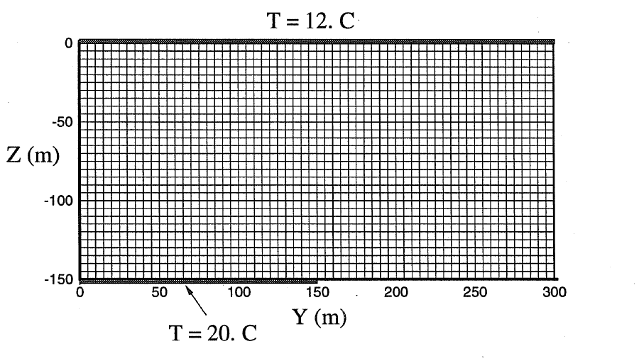
Figure 1: The experiment schematic (Oldenburg et al., 1995).
Input file setup
This section describes the input file syntax.
Mesh
The first step is to set up the mesh. In this problem, a rectangular tank with a width of 300 m and a height of 150 m is simulated. For convenience, instead of the YZ coordinate as shown in Figure 1, the simulation was set up in XY coordinate with the positive Y direction pointing toward the top of the tank. In this code block, the numbers of nodes in the X and Y directions are specified along with the dimension of the tank. A notable feature is the declaration of the boundary heater. This is due to the fact that the heat element at the bottom of the tank is located between 0< x < 150 m. This enables simple boundary condition implementation at later stages.
[Mesh]
  [gen]
    type = GeneratedMeshGenerator
    dim = 2
    nx = 64
    ny = 32
    xmin = 0
    xmax = 300
    ymax = 0
    ymin = -150
  []
  [heater]
    type = ParsedGenerateSideset
    input = gen
    combinatorial_geometry = 'x <= 150 & y = -150'
    new_sideset_name = heater
  []
  uniform_refine = 1
[]
Fluid properties
After the mesh has been specified, we need to provide the fluid properties that are used for this simulation. For our case, it will be just water and can be easily implemented as follows:
[FluidProperties]
  [water]
    type = Water97FluidProperties
  []
[]
Variables declaration
Since we are focusing on the natural convection of flow in a porous medium, temperature (T) and porepressure are used.
[Variables]
  [porepressure]
  []
  [T]
    initial_condition = 285
  []
[]
Action declaration
For this problem, we use the PorousFlowFullySaturated to automatically add all of the physics kernels and a number of the necessary material properties. As this is a TH problem, we set coupling_type = Thermohydro.
[PorousFlowFullySaturated]
  coupling_type = ThermoHydro
  porepressure = porepressure
  temperature = T
  fp = water
[]
Additional material properties not added by the action are specified in the Materials block.
[Materials]
  [porosity]
    type = PorousFlowPorosityConst
    porosity = 0.1
  []
  [permeability]
    type = PorousFlowPermeabilityConst
    permeability = '1.21E-10 0 0   0 1.21E-10 0   0 0 1.21E-10'
  []
  [Matrix_internal_energy]
    type = PorousFlowMatrixInternalEnergy
    density = 2500
    specific_heat_capacity = 0
  []
  [thermal_conductivity]
    type = PorousFlowThermalConductivityIdeal
    dry_thermal_conductivity = '1.5 0 0  0 1.5 0  0 0 0'
  []
[]
Initial and Boundary Conditions
The next step is to supply the initial and boundary conditions. For this problem, two initial conditions need to be implemented. The first one is a constant temperature of 285 K which was declared in the previous section. The second one is the hydrostatic variation of porepressure along the y direction as shown below:
[ICs]
  [hydrostatic]
    type = FunctionIC
    variable = porepressure
    function = '1e5 - 9.81 * 1000 * y'
  []
[]
Shifting to the boundary conditions. There are three Dirichlet boundary conditions that we need to supply. The first two are constant temperature at the top and heater surfaces denoted as t_top and t_bot. And, the last one is constant pressure at the top surface denoted as p_top.
[BCs]
  [t_bot]
    type = DirichletBC
    variable = T
    value = 293
    boundary = 'heater'
  []
  [t_top]
    type = DirichletBC
    variable = T
    value = 285
    boundary = 'top'
  []
  [p_top]
    type = DirichletBC
    variable = porepressure
    value = 1e5
    boundary = top
  []
[]
Executioner setup
Lastly, we will tell Moose the type of the problem (shown in the code block below). For this problem, a transient solver is required. To save time and computational resources, IterationAdaptiveDT and mesh Adaptivity were implemented. The former enables the time step to be increased if the solution converges and decreased if it does not. This will help save time if a large time step can be used and aid in convergence if a small time step is required. Similarly, the latter enables the mesh to automatically adapt to optimize the computational resource usage and resolve the area with stiff gradients. The mesh will be coarsened at the regions with low error and refined at the critical areas (high error and stiff gradients). For practice, users can try to disable them by putting the code block into comment and witnessing the difference in the solving time and solution.
[Executioner]
  type = Transient
  end_time = 63072000
  dtmax = 1e6
  nl_rel_tol = 1e-6
  [TimeStepper]
    type = IterationAdaptiveDT
    dt = 1000
  []
  [Adaptivity]
    interval = 1
    refine_fraction = 0.2
    coarsen_fraction = 0.3
    max_h_level = 4
  []
[]
Auxiliary kernels and variables (optional)
This section is optional since these kernels and variables do not affect the calculation of the desired variable. In this example, we want to output the fluid density at the end of the simulation thus we will add an auxkernel and an auxvariable for it. It can be noticed that the term execute_on = TIMESTEP_END indicates this kernel will be activated to calculate the fluid density at the end of each time step only, thus this calculation does not affect the performance of other tasks.
[AuxVariables]
  [density]
    family = MONOMIAL
    order = CONSTANT
  []
[]
[AuxKernels]
  [density]
    type = PorousFlowPropertyAux
    variable = density
    property = density
    execute_on = TIMESTEP_END
  []
[]
Result
The input file can be executed and the result is as follows:
Figure 2: Spatial distribution of temperature with a test time of 2 years.
It is obvious that the mesh at the interface between hot and cold fluid is much more refined as discussed while surrounding areas have a coarser mesh.
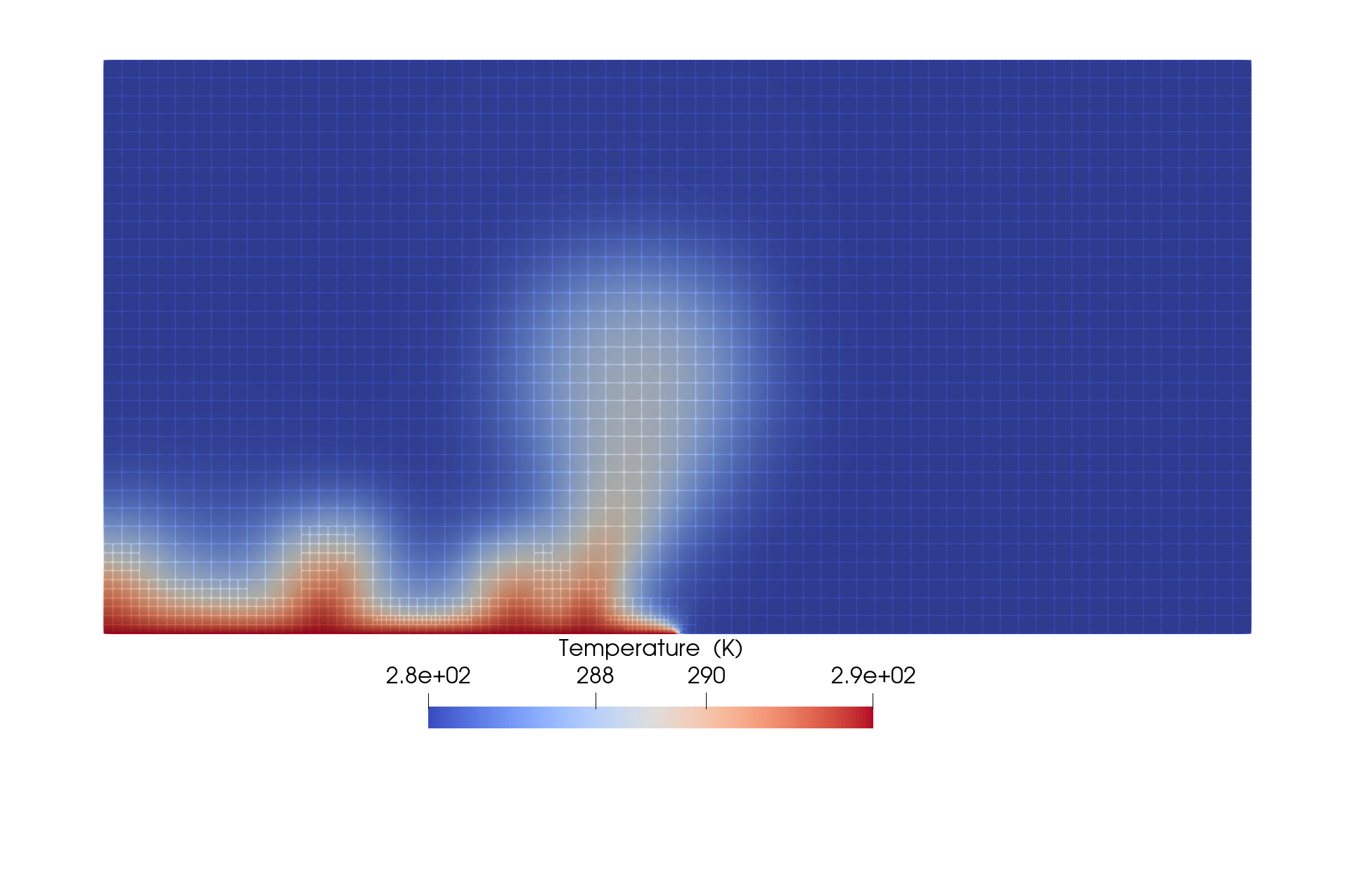
Figure 3: Spatial distribution of temperature at the end of 2 years with mesh grid displayed.
The result from the simulation agrees well with published literature.
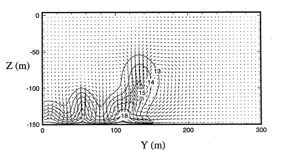
Figure 4: Temperature contours and velocity vectors after 2 years (Oldenburg et al., 1995).
References
- Jacob W. Elder.
Transient convection in a porous medium.
Journal of Fluid Mechanics, 27:609 – 623, 1967.
URL: https://api.semanticscholar.org/CorpusID:123656493.[BibTeX]
- C. M. Oldenburg, Ruth L. Hinkins, George J. Moridis, and Karsten Pruess.
On the development of mp-tough2.
Technical Report, Lawrence Berkeley National Laboratory, 1995.
URL: https://api.semanticscholar.org/CorpusID:59668502.[BibTeX]