Electrostatic Contact Verification (Two Block Test)
This document describes the two block 1-D verification test for the ElectrostaticContactCondition object. Below is a summary of the test, along with a derivation of the analytic solution used for comparison and the relevant test input file for review.
Summary
A visual summary of the two block verification test domain, as well as relevant boundary and interface conditions is shown below (click to zoom):
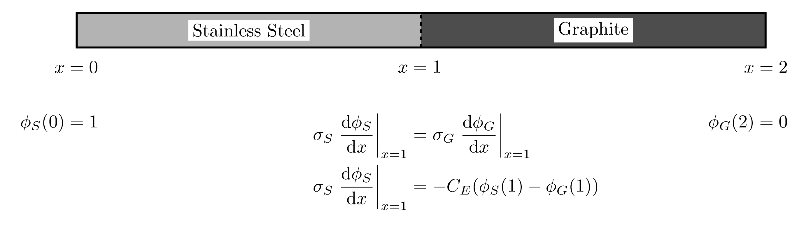
Figure 1: Visual summary of the two block verification test with boundary and interface conditions.
It is important to note that in Figure 1:
is the electrical conductivity of material ,
is the electrical contact conductance at the interface, and
is the electrostatic potential of material .
See the ElectrostaticContactCondition documentation for more information about the particular definition of . As the ElectrostaticContactCondition object is intended for electrostatic field solves, the PDE being solved within each domain is Poisson's Equation for electrostatic potential. In this case, we are assuming a zero total charge density, which leads to
(1)Material properties being used in this case are constants in each block, and they are summarized below in Table 1. All material properties were evaluated at a temperature of ~300 K.
Table 1: Material properties for the two block electrostatic contact verification case.
| Property (unit) | Value | Source |
|---|---|---|
| Stainless Steel (304) Electrical Conductivity (S / m) | (Cincotti et al., 2007) | |
| Stainless Steel (304) Hardness (Pa) | (Cincotti et al., 2007) | |
| Graphite (AT 101) Electrical Conductivity (S / m) | (Cincotti et al., 2007) | |
| Graphite (AT 101) Hardness (Pa) | (Cincotti et al., 2007) |
The hardness values shown in Table 1 are used in the ElectrostaticContactCondition object as a harmonic mean of the two values. For reference, the harmonic mean calculation for two values, and , is given by
In the input file, the harmonic mean of hardness for stainless steel and graphite was calculated and set to be Pa.
Analytic Solution Derivation
In 1-D, Eq. (1) becomes
since is constant in both domains. This equation means a reasonable guess for a generic solution function for would be
where and are to-be-determined constant coefficients.
Apply boundary conditions
Using the boundary conditions in Figure 1, we can determine for both the stainless steel and graphite regions:
Stainless Steel
Graphite
Apply interface conditions
Now, the interface conditions can be applied from Figure 1. To begin, let's focus on the current density () equivalence condition
Taking into account our initial guess for the solution function, this becomes
(2)Next, we can apply the conductance condition from Figure 1, which is
Taking into account our initial guess for the solution function and the constant coefficients solved for above, this becomes
(3)
Find the remaining coefficients
Using the Elimination Method, we can combine Eq. (2) and Eq. (3) in order to solve for each remaining unknown coefficient. If Eq. (2) is multiplied through on both sides by and Eq. (3) is multiplied through on both sides by , we have
and
Grouping terms, we then have
(5)Combining Eq. (4) and Eq. (5) together via addition yields
which can then be solved for
Using Eq. (2), can now be solved for
Summarize
Now our determined coefficients can be combined to form the complete solutions for both stainless steel and graphite. To summarize, the derived analytical solutions for each domain given the boundary and interface conditions described in Figure 1 is
This is implemented in source code as ElectricalContactTestFunc.C and is located within the test source code directory located at modules/electromagnetics/test/src.
Input File
# Regression test for ElectrostaticContactCondition with analytic solution with
# two blocks
#
# dim = 1D
# X = [0,2]
# Interface at X = 1
#
#   stainless_steel        graphite
# +------------------+------------------+
#
# Left BC: Potential = 1
# Right BC: Potential = 0
# Center Interface: ElectrostaticContactCondition
#

[Mesh]
  [line]
    type = GeneratedMeshGenerator
    dim = 1
    nx = 4
    xmax = 2
  []
  [break]
    type = SubdomainBoundingBoxGenerator
    input = line
    block_id = 1
    block_name = 'graphite'
    bottom_left = '1 0 0'
    top_right = '2 0 0'
  []
  [block_rename]
    type = RenameBlockGenerator
    input = break
    old_block = 0
    new_block = 'stainless_steel'
  []
  [interface]
    type = SideSetsBetweenSubdomainsGenerator
    input = block_rename
    primary_block = 'stainless_steel'
    paired_block = 'graphite'
    new_boundary = 'ssg_interface'
  []
[]

[Variables]
  [potential_graphite]
    block = graphite
  []
  [potential_stainless_steel]
    block = stainless_steel
  []
[]

[AuxVariables]
  [analytic_potential_stainless_steel]
    block = stainless_steel
  []
  [analytic_potential_graphite]
    block = graphite
  []
[]

[Kernels]
  [electric_graphite]
    type = ADMatDiffusion
    variable = potential_graphite
    diffusivity = electrical_conductivity
    block = graphite
  []
  [electric_stainless_steel]
    type = ADMatDiffusion
    variable = potential_stainless_steel
    diffusivity = electrical_conductivity
    block = stainless_steel
  []
[]

[AuxKernels]
  [analytic_function_aux_stainless_steel]
    type = FunctionAux
    function = potential_fxn_stainless_steel
    variable = analytic_potential_stainless_steel
    block = stainless_steel
  []
  [analytic_function_aux_graphite]
    type = FunctionAux
    function = potential_fxn_graphite
    variable = analytic_potential_graphite
    block = graphite
  []
[]

[BCs]
  [elec_left]
    type = ADDirichletBC
    variable = potential_stainless_steel
    boundary = left
    value = 1
  []
  [elec_right]
    type = ADDirichletBC
    variable = potential_graphite
    boundary = right
    value = 0
  []
[]

[InterfaceKernels]
  [electric_contact_conductance_ssg]
    type = ElectrostaticContactCondition
    variable = potential_stainless_steel
    neighbor_var = potential_graphite
    boundary = ssg_interface
    mean_hardness = mean_hardness
    mechanical_pressure = 3000
  []
[]

[Materials]
  #graphite (at 300 K)
  [sigma_graphite]
    type = ADGenericConstantMaterial
    prop_names = electrical_conductivity
    prop_values = 73069.2
    block = graphite
  []

  #stainless_steel (at 300 K)
  [sigma_stainless_steel]
    type = ADGenericConstantMaterial
    prop_names = electrical_conductivity
    prop_values = 1.41867e6
    block = stainless_steel
  []

  # harmonic mean of graphite and stainless steel hardness
  [mean_hardness]
    type = ADGenericConstantMaterial
    prop_names = mean_hardness
    prop_values = 2.4797e9
  []
[]

[Functions]
  [potential_fxn_stainless_steel]
    type = ElectricalContactTestFunc
    domain = stainless_steel
  []
  [potential_fxn_graphite]
    type = ElectricalContactTestFunc
    domain = graphite
  []
[]

[Postprocessors]
  [error_stainless_steel]
    type = ElementL2Error
    variable = potential_stainless_steel
    function = potential_fxn_stainless_steel
    block = stainless_steel
  []
  [error_graphite]
    type = ElementL2Error
    variable = potential_graphite
    function = potential_fxn_graphite
    block = graphite
  []
[]

[Preconditioning]
  [SMP]
    type = SMP
    full = true
  []
[]

[Executioner]
  type = Steady
  solve_type = NEWTON
  automatic_scaling = true
[]

[Outputs]
  csv = true
  perf_graph = true
[]
Results
Results from the input file shown above (with Mesh/line/nx=30 and Outputs/exodus=true) compared to the analytic function are shown below in Figure 2. Note that the number of points shown in the plot has been down-sampled compared to the solved number of elements for readability.
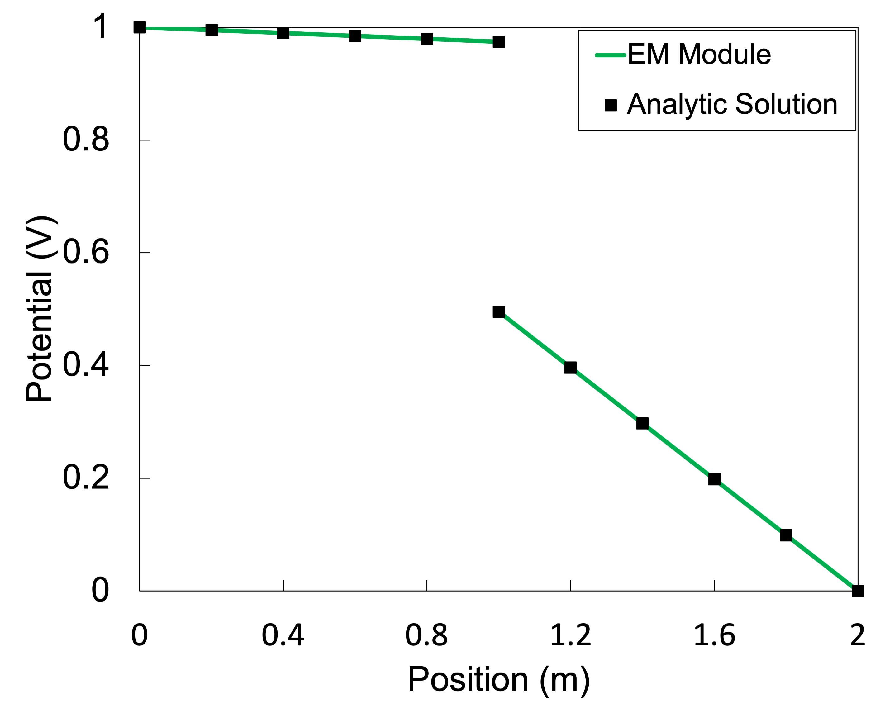
Figure 2: Results of electrostatic contact two block validation case.
References
- A. Cincotti, A. M. Locci, R. Orrù, and G. Cao.
Modeling of SPS apparatus: temperature, current and strain distribution with no powders.
AIChE Journal, 53(3):703–719, 2007.
doi:10.1002/aic.11102.[BibTeX]