XFEM Module Theory
The MOOSE XFEM module is a library for the implementation of the extended finite element method (XFEM) that solves partial differential equations (PDEs) with some form of discontinuity. For an overview of the XFEM fracture capability, please see the journal article Jiang et al. (2020).
Phantom-node-based XFEM
The XFEM approach as originally proposed Belytschko and Black (1999) and Moës et al. (1999) enriches the standard continuous finite element interpolation of the solution field as a function of spatial coordinate and time with Heaviside and near-tip enrichment functions: where is the number of nodes per finite element, are the standard finite element interpolation functions, are the nodal displacements, is the Heaviside function, are additional nodal degrees of freedom corresponding to Heaviside enrichment, are a set of enrichment functions that capture asymptotic near-tip fields, and are additional nodal degrees of freedom corresponding to the near-tip enrichment. This approach requires an additional degree of freedom per solution variable for each node whose support is traversed by a crack for Heaviside enrichment, as well as 4 additional degrees of freedom per solution variable for the nodes in the vicinity of the crack tip to which near-tip enrichment is applied. The set of enriched nodes is typically a small subset of the nodes in the discretized solution because a small fraction of the solution domain is typically directly affected by cracking. As a result, this does not drastically increase the number of unknowns in the system of equations. However, this can be difficult to implement in existing FEM codes if they do not permit nodes to have arbitrary number of degrees of freedom.
The phantom node method Hansbo and Hansbo (2004) was also proposed as a technique for modeling mesh-independent fracture. In the phantom node method, elements intersected by a crack are deleted and replaced by two elements that occupy the same physical locations as the original elements. A portion of the domain of each of these new elements (partial elements) represents physical material. The combined physical portions of the partial elements cover the entire domain of the original element that was split. The nodes connected to the non-physical portions of those elements are known as phantom nodes. The solution field is interpolated on the partial elements using the standard finite element shape functions. When fields are integrated on partial elements, as is done to compute an element's contribution to the residual, the integral is only performed over the physical part of the element. Shortly after the phantom node technique was proposed, it was shown Areias and Belytschko (2006) to give exactly the same enrichment as the originally proposed XFEM (without the near-tip enrichment functions), and add the same number of extra degrees of freedom to the system to represent discontinuities.
The phantom node technique has several features that make it more attractive than the originally-proposed XFEM for a Heaviside enrichment capability from an implementation standpoint:
It is generally less invasive on a host FEM code architecture because it does not require the addition of nonstandard degrees of freedom, and requires only minor modifications to the element integration procedures.
The additional degrees of freedom correspond to standard solution fields, which aids in interpretation of results.
It simplifies the handling of crack branching and coalescence, which require additional degrees of freedom in elements containing multiple cracks in the original XFEM, but can be handled by recursively cutting elements in the phantom node method Song and Belytschko (2009) and Richardson et al. (2011).
For multiphysics applications where the physics applications share a common mesh, the phantom node technique automatically enriches the degrees of freedom for all solution variables, whereas additional enrichment degrees of freedom would need to be explicitly added in the original XFEM.
Mesh Cutting Algorithm
The bulk of the complexity in implementing the phantom node method lies in correctly resolving the connectivity of the partial elements that are created when elements are cut by a crack. Neighboring elements that share a common cracked edge should share physical and phantom nodes to ensure continuity of finite element solution fields in across neighboring elements in the material on a given side of a crack. Conversely, the elements on opposing sides of a crack should have no connectivity to ensure that the discontinuity is properly represented. Figure 1 and Figure 2 illustrate the desired connectivity for a representative crack geometry. An algorithm based partly on the work of Richardson et al. Richardson et al. (2011) was developed for the present work, and is described here. Because this cutting algorithm relies on the use of data structures known as fragments, it is termed here as the element fragment algorithm (EFA).
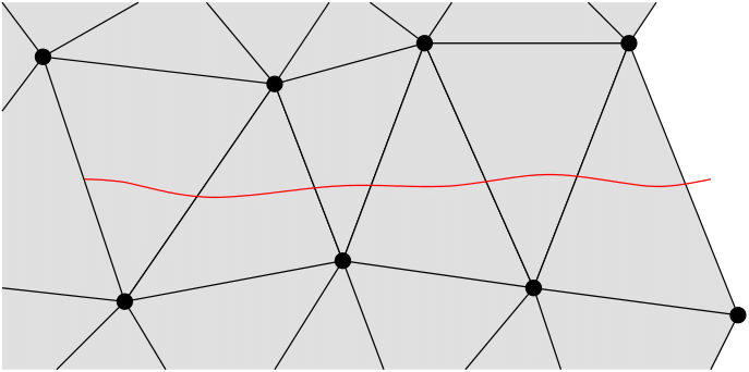
Figure 1: Original mesh with prescribed cutting line shown in red.
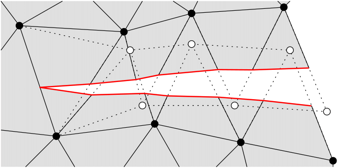
Figure 2: Cut mesh showing phantom nodes and partial elements.
Fracture mechanics problems impose important requirements on the behavior of the cutting algorithm at crack tips. In general, the XFEM permits a crack tip to be located anywhere in the solution domain, including within finite elements. If only Heaviside enrichment is used, however, crack tips must coincide with finite element boundaries. To properly represent the topology at crack tips, the cut edges of the partial elements representing the material on opposing sides of the crack must be merged with the uncut element ahead of the crack tip. This can be seen in Figure 2. In addition, to represent cracks that propagate over time, as a crack advances into a new element, the merged edges of those elements that were previously at the crack tip must be disconnected.
This special handling of propagating cracks introduces additional complexity to the cutting algorithm. One could avoid this by simply discarding the cut mesh every time cracks advance and cut a copy of the original mesh. However, in simulations where stateful material data is associated with element integration points, it is important to not discard the cut elements, because they contain unique material data that would be lost if the cut mesh were deleted. For this reason, the algorithm described here is designed to operate on the cut mesh in its previous cut state every time the mesh is to be modified to extend existing cracks or initiate new cracks. This approach also has the advantage that it avoids the memory requirements of storing the uncut mesh.
Data Structure and Terminology
The EFA uses a mesh data structure that consists of elements connected by nodes, just like a finite element mesh. It does not explicitly require the nodal coordinates because it only deals with the connections between elements, and not the physical locations of those elements. An implementation of this algorithm could use the same finite element data structures used by the host code, but in the present work, a separate mesh is used for the EFA. This allows features specific to this algorithm to be added to the data structure without impacting the rest of the host finite element code.
Describing the EFA requires the definition of some unique terminology:
Cutting Plane: These are geometric planes used to define locations of discontinuities represented by XFEM. These can be defined in a number of ways, such as through simple geometric descriptions or level set functions. These can evolve as indicated by physics-based criteria such as stresses or fracture integrals that indicate how that cracks should extend.
Child Element: Every element that is traversed by a cutting plane is replaced by multiple new elements, which are denoted as child elements.
Parent Element: The elements that are replaced by child elements when traversed by cutting planes are known as parent elements.
Crack Tip Element: Elements immediately ahead of the crack tip (which is represented by two partial elements that are both connected to the same uncut face of a neighboring element) are denoted as crack tip elements.
Crack Tip Split Element: The partial elements just behind the crack tip that overlap another partial element that is merged with a common element face at the crack tip are called crack tip split elements.
Child Node: As child elements are created to replace parent elements, some of the nodes in these child elements are new nodes that overlay existing nodes. These are known as child nodes.
Parent Node: The nodes that are duplicated to give rise to child nodes are known as parent nodes.
Embedded Node: These are additional nodes that are created at the intersections of cutting planes with finite element edges or other cutting planes. These nodes are globally numbered like standard finite element nodes, but are not associated with degrees of freedom in the discretized equation system. They are used for bookkeeping in the EFA.
Fragment: The portion of a cut finite element representing the material located on one side of one or more cutting planes is known as a fragment. An element could potentially be cut by multiple cutting planes, and the fragments represent the smallest quantities of uncut material within an element. The union of the fragments in a given set of child elements completely covers the domain of their original parent element. Fragments are defined by the set of line segments that make up their perimeter in 2D or by the set of faces that make up their boundary in 3D. The line segments connect nodes, which can be either embedded nodes or permanent nodes (defined later). A new child element is created for each fragment in the parent element, and each child element contains exactly one fragment.
Temporary Node: When child elements are created, new nodes are created at the locations of all nodes that are not contained within a fragment (i.e. connected to physical material). These new nodes are known as temporary nodes. These temporary nodes are ultimately merged with other nodes as connectivities are determined, and are either deleted or converted to become permanent nodes (defined later), so that after the EFA is complete, there are no remaining temporary nodes.
Permanent Node: Permanent nodes are the finite element nodes that remain after the EFA is complete. These nodes may or may not be connected to physical material. All permanent nodes are associated with degrees of freedom in the global system of equations.
Phantom Node: Phantom nodes are a subset of the physical nodes, and are the nodes not connected to any physical material. They are not actually handled any differently than other finite element nodes, and there is no need to designate nodes as being phantom nodes in the algorithmic implementation, but for understanding the EFA and its outcomes, it can be helpful to describe nodes as being phantom nodes.
Algorithmic Flow
The EFA is designed to be called repeatedly during an analysis to represent dynamically evolving crack topologies. As illustrated in Figure 3 and also outlined in Zhang (2015), each time the mesh is to be modified, the following steps are taken:
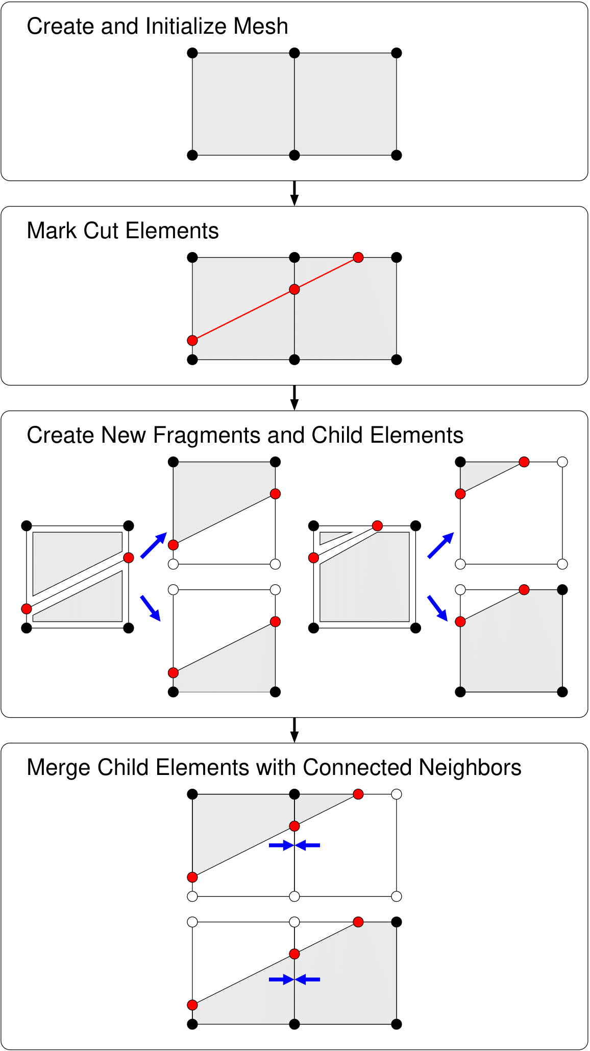
Figure 3: High level flow chart illustrating the steps in the EFA.
Create and Initialize Mesh: The mesh structure for the EFA is populated with elements and nodes corresponding to those in the host code. If the mesh has been previously cut by the EFA, the topology of the cut mesh, rather than the original mesh is used. Any information about fragments and embedded nodes from the previous cut state is also restored. Neighboring elements connected to all elements in this cut mesh, as well as the current crack tip elements and crack tip split elements, are identified.
Mark Cut Elements: Elements newly intersected by cutting planes are identified, and new embedded nodes are created at the locations on the edges that are intersected. The determination of whether elements are cut and identification of locations of intersections of planes with element edges are performed in the host code. The embedded node locations are defined in the EFA in terms of the edges on which they are located and the fractional distances on those edges. The distances on the edges are necessary to disambiguate which embedded node corresponds to a cutting plane when multiple cuts intersect an element edge. This scenario is naturally handled by this algorithm, but is not discussed in detail here.
Create New Fragments and Child Elements: Once all cut elements are identified, new fragments are created for each continuous region within an uncut element, and a new child element is created corresponding to each fragment. Figure 4 illustrates this process. New temporary nodes are created as children of the original nodes in the portions of the child elements outside of fragments, while the original permanent nodes are used when a node is contained within a fragment. Crack tip elements have one or more edge (in 2D) or face (in 3D) intersected by a cutting plane that terminates at, but does not traverse the element. These elements have a single fragment created, which contains the embedded node (2D) or nodes (3D), and a single new element is created corresponding to that fragment. The element on the far right of Figure 5 is an example such an element.
Merge Child Elements with Connected Neighbors: The last phase of this algorithm is to merge the newly-created child elements with neighboring elements as appropriate, which is done by merging nodes on the common edge of the two elements. Neighboring elements are merged if they have a material connection, which means they share a common edge (2D) or face (3D) that has physical material connected to a common portion of it on both elements. The fragments are used for making this determination. If the fragments in two neighboring elements share a common edge (2D) or face (3D), the elements are deemed to have a material connection, and the nodes on the edge or face containing that connection should be merged. This ensures that there is spatial continuity in the solution variables in that region, as is appropriate for representing a continuous material.
A few rules are followed when merging nodes on common edges. If a temporary node is merged with a permanent node, it deleted and replaced by the permanent node. If two temporary nodes are merged, they are both deleted and replaced with a single newly-created permanent node. Finally, there are some special scenarios in which two permanent nodes are to be merged and have differing indices. This can occur at nodes on the edge or face where a crack terminates if those nodes are also connected to another edge or face traversed by the crack behind the crack tip. In such cases, one of those nodes is always a child of the other node. The child node is deleted and replaced with the permanent node.
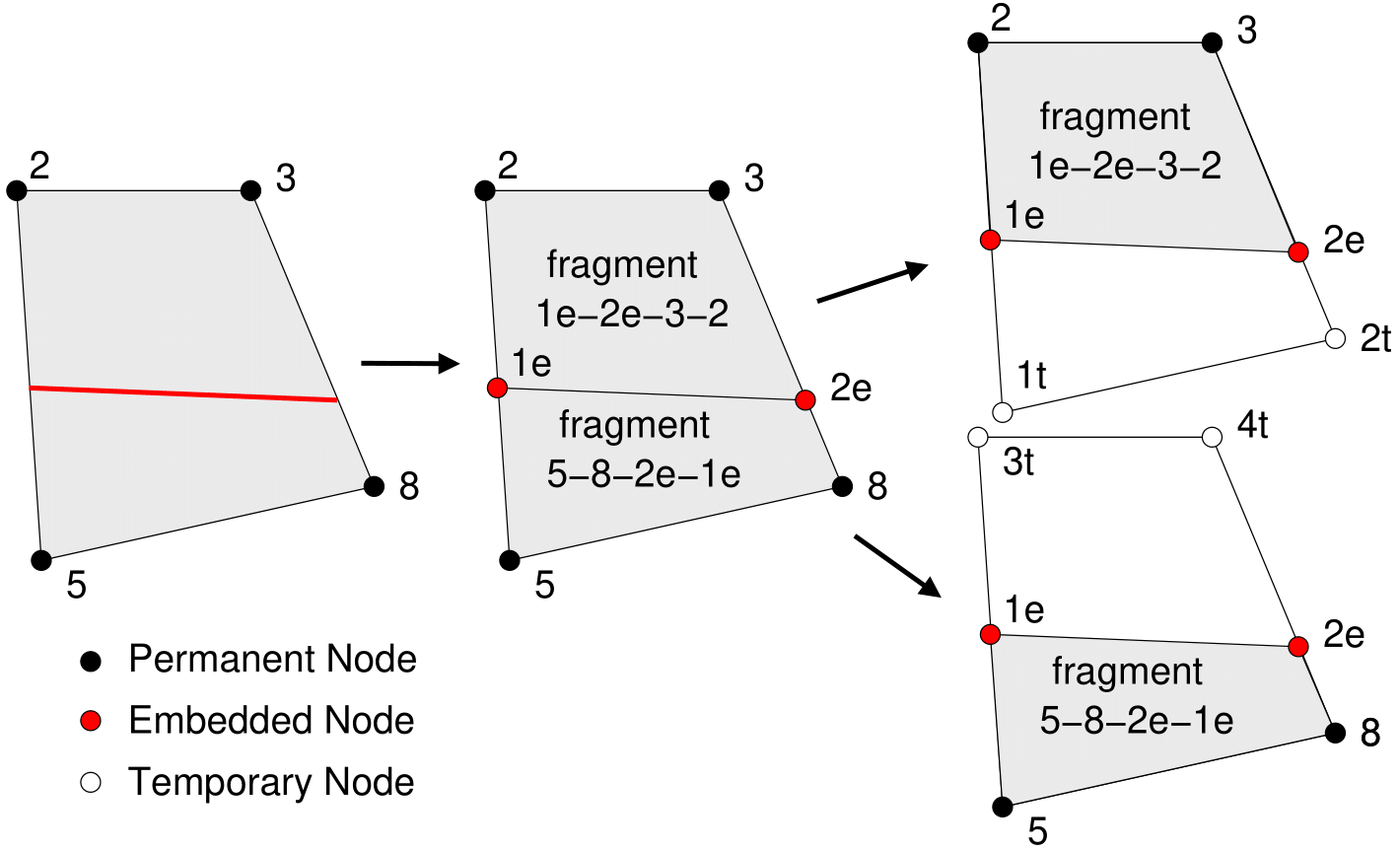
Figure 4: Illustration of the process of marking and splitting an element. First, it is determined that the element is intersected by a cutting plane (left). Embedded nodes (denoted with an "e") are then created at intersections of element edges with the cutting plane, and fragments are created for each continuous region within the cut element (middle). Fragments are identified by the set of edges defining their boundaries. Finally, a new child element is created corresponding to each fragment, with new temporary nodes (denoted with a "t") to replace all nodes that are not connected to a fragment (right).
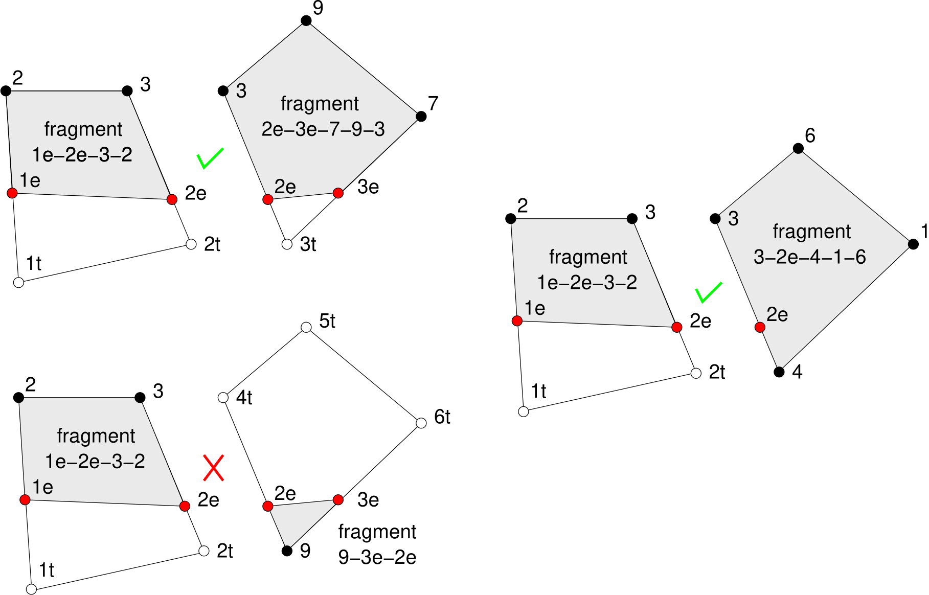
Figure 5: Determination of whether two neighboring elements share a material connection and should be merged on a common edge. The two elements in the upper left are merged because their fragments share a common edge (3-2e). The fragments in the elements in the lower left do not share any common edges, so those elements are not merged. The scenario on the right shows how the crack tip split element on the left should be merged with a crack tip element on the right because their fragments share a common edge (3-2e).
When this algorithm is completed, all temporary nodes should be deleted and replaced by permanent nodes. The EFA generates a set of new child nodes and a set of new child elements to be created, as well as a set of parent elements to be deleted. The new child elements and nodes are all associated with their parents, so that material data can be transferred to the child elements and nodal solution data can be transferred to the child nodes. Figure 7 shows the full process of the EFA demonstrated on a patch of elements partially intersected by a cutting plane. The resulting mesh represents two crack tips at the ends of the cutting plane.
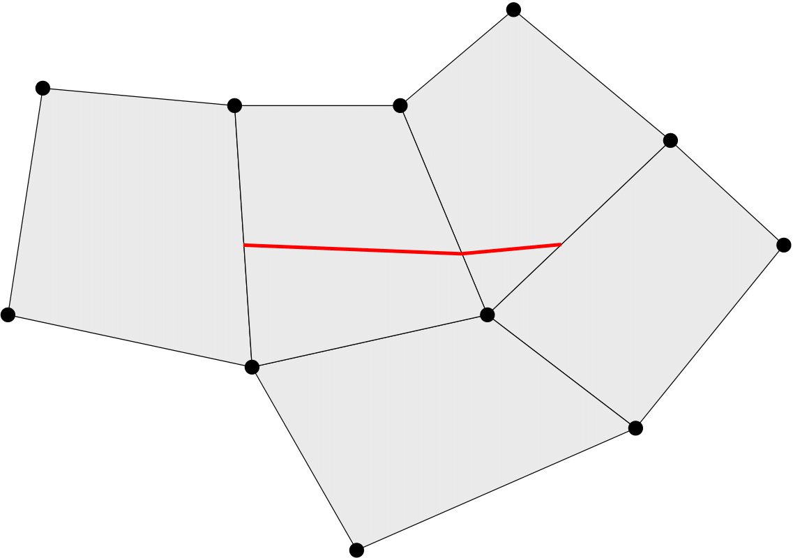
Figure 6: Identification of cut locations and cut edges.
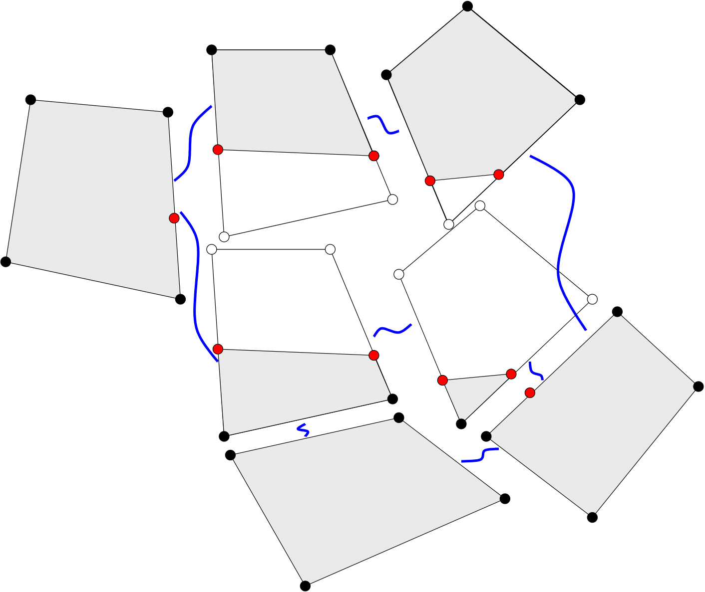
Figure 7: Replacement of cut elements with partial elements and identification of edges to be combined because of shared material (shown by blue lines).
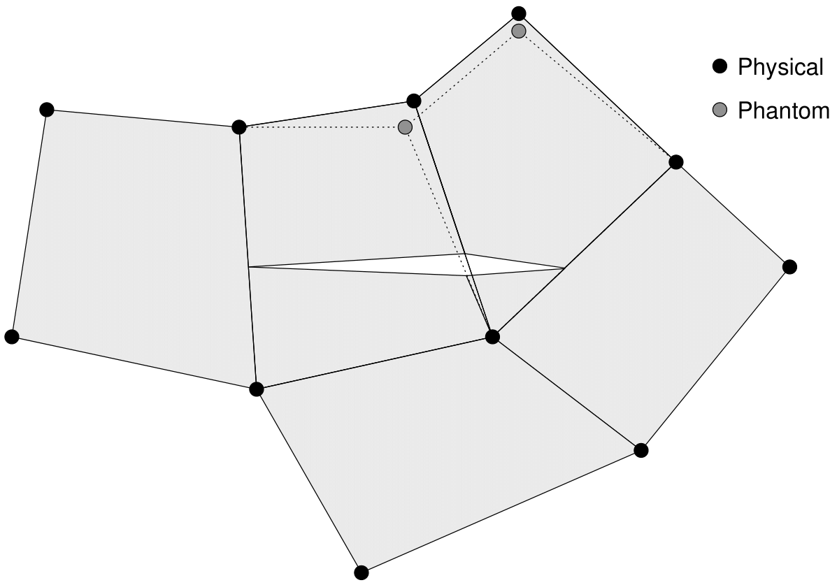
Figure 8: Final modified mesh. Phantom nodes are those that are not connected to physical material.
As mentioned previously, for this algorithm to permit the extension of cracks using the state of the mesh cut in a previous step, special treatment of the crack tip split elements is required to disconnect the nodes that were shared on the edge (2D) or face (3D) where the crack tip was previously located. In step 3 of the algorithm described above, elements that were previously split by a cutting plane are usually left alone, with no new fragments or child elements created. In the special case where a crack will fully cut a crack tip element, however, the crack tip split elements adjacent to that element each create a single new child element containing the same fragment that was present prior to this step. This results in the creation of new temporary nodes, which are merged with other nodes using the standard procedure.
Although the EFA is illustrated here using a 2D mesh and the applications shown in this paper are limited to 2D, this algorithm is readily applicable to 3D models. When there are distinctions between the 2D and 3D cases, those have been described in the above description of the algorithm, and these generally are related to the use of higher dimensionality geometric primitives (e.g. faces instead of edges) for the 3D case. Also, this is not directly an issue with the EFA, but when extending this approach to 3D, there are other challenges such as continuity of the cutting planes between adjacent cracked elements Duan et al. (2009) that must also be addressed.
Finally, it should be noted that in the EFA as described above, if two child elements cut by the same crack have an edge that their parents share in common, but that edge contains no physical material, the nodes on that edge are not merged. This results in an extra phantom node, and hence an extra degree of freedom for every solution variable at that node. This behavior differs from the original XFEM, which would only add one degree of freedom to that node per field variable component. This scenario is shown on the patch of elements shown in Figure 9. The MOOSE implementation of this algorithm provides an option to merge these edges to recover the original XFEM behavior, and this is used in the present work.
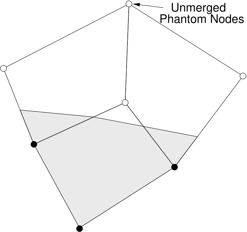
Figure 9: Scenario in which the unmodified element fragment algorithm results in extra degrees of freedom. Without special treatment, there are two coincident phantom nodes at the indicated location because the neighboring edges share no physical material.
Partial Element Integration Algorithm
Aside from the mesh cutting algorithm, the other major modification that must be made to the finite element code for the phantom node algorithm is that quadrature rules that are used to perform volume integrals, such as for computing the integral of the divergence of the stress tensor to compute an element's contribution to the residual, are adjusted to integrate over the physical portions of the cut elements. This is commonly done by forming a set of triangular (2D) or tetrahedral (3D) sub-elements that cover the entire physical portion of the split element's domain. These sub-elements are used only for integration, and new integration points are introduced at the locations of those sub-elements' integration points.
A significant drawback of this sub-division approach to partial element integration is that when there is stateful material data at integration points (as is often the case for nonlinear mechanical constitutive models and a variety of other behavior models used in fuel performance analysis), this data must be mapped to the new integration points. There are approaches to integration of partial elements that avoid this mapping of material data to new integration points by using the original integration points, but scaling the weight factors in the numerical integration procedure to give a reasonable approximation of the integration of a function over a portion of the domain. The simplest approach is to simply scale the weights by a factor equal to the physical volume fraction of a split element. A more sophisticated approach known as moment fitting uses a least squares procedure to compute separate weights for each integration point to optimally integrate a specified set of functions. A recent study by Zhang et al. (2018) shows on a variety of problems that the moment fitting approach gives results that are slightly improved over the simple volume fraction approach, and that both approaches are viable on problems of practical interest. The moment fitting scheme described in that work is used with a four-point integration rule for the 2D linear quadrilateral elements used in the present study.
Visualization of Results
The mesh-cutting algorithm and the partial element integration scheme are the only major changes to a finite element code that are strictly necessary for an XFEM implementation using the phantom node algorithm. However, because the phantom node approach replaces each cut element with overlapping elements, it is also very helpful during visualization to show only the physical portions of cut elements, as the non-physical portions of those elements can obscure the results of interest. It is important to note that in the phantom node approach, the actual displacement fields are directly computed, and there is no need to modify the visualized results beyond clipping the non-physical portions of cut elements to account for enrichment, as is necessary in the original XFEM. XFEM Paraview Plugin (MooseXfemClip) is developed to visualize results produced by the XFEM in the MOOSE. MooseXfemClip is available in Paraview software as an optional plugin. Users can load it in the Paraview's Plugin Manager setting.
References
- P.M.A. Areias and T. Belytschko.
A comment on the article “A finite element method for simulation of strong and weak discontinuities in solid mechanics” by A. Hansbo and P. Hansbo Comput. Methods Appl. Mech. Engrg. 193 (2004) 3523-3540.
Computer Methods in Applied Mechanics and Engineering, 195(9-12):1275–1276, 2006.
doi:http://dx.doi.org/10.1016/j.cma.2005.03.006.[BibTeX]
- T. Belytschko and T. Black.
Elastic crack growth in finite elements with minimal remeshing.
International Journal for Numerical Methods in Engineering, 45(5):601–620, June 1999.
doi:10.1002/(SICI)1097-0207(19990620)45:5<601::AID-NME598>3.0.CO;2-S.[BibTeX]
- Qinglin Duan, Jeong-Hoon Song, Thomas Menouillard, and Ted Belytschko.
Element-local level set method for three-dimensional dynamic crack growth.
International Journal for Numerical Methods in Engineering, 80(12):1520–1543, 2009.[BibTeX]
- Anita Hansbo and Peter Hansbo.
A finite element method for the simulation of strong and weak discontinuities in solid mechanics.
Computer Methods in Applied Mechanics and Engineering, 193(33):3523 – 3540, 2004.
doi:https://doi.org/10.1016/j.cma.2003.12.041.[BibTeX]
- Wen Jiang, Benjamin W. Spencer, and John E. Dolbow.
Ceramic nuclear fuel fracture modeling with the extended finite element method.
Engineering Fracture Mechanics, 223:106713, 2020.
URL: http://www.sciencedirect.com/science/article/pii/S0013794419307568, doi:https://doi.org/10.1016/j.engfracmech.2019.106713.[BibTeX]
- Nicolas Moës, John Dolbow, and Ted Belytschko.
A finite element method for crack growth without remeshing.
International Journal for Numerical Methods in Engineering, 46(1):131–150, 1999.
doi:10.1002/(SICI)1097-0207(19990910)46:1<131::AID-NME726>3.0.CO;2-J.[BibTeX]
- Casey L. Richardson, Jan Hegemann, Eftychios Sifakis, Jeffrey Hellrung, and Joseph M. Teran.
An XFEM method for modeling geometrically elaborate crack propagation in brittle materials.
International Journal for Numerical Methods in Engineering, 88(10):1042–1065, 2011.
doi:10.1002/nme.3211.[BibTeX]
- Jeong-Hoon Song and Ted Belytschko.
Dynamic Fracture of Shells Subjected to Impulsive Loads.
Journal of Applied Mechanics, 06 2009.
051301.
URL: https://doi.org/10.1115/1.3129711.[BibTeX]
- Ziyu Zhang.
Finite Element Methods for Interface Problems with Mesh Adaptivity.
PhD thesis, Duke University, 2015.[BibTeX]
- Ziyu Zhang, Wen Jiang, John E. Dolbow, and Benjamin W. Spencer.
A modified moment-fitted integration scheme for X-FEM applications with history-dependent material data.
Computational Mechanics, 62(2):233–252, August 2018.
doi:10.1007/s00466-018-1544-2.[BibTeX]