Tidal impacts on porepressure
The porepressure in underground porous materials is influenced by external factors, such as earth tides, barometric pressure changes, and oceanic tides. The response of porepressure to these factors can help quantify important hydrogeological parameters, such as the poroelastic constants and even the permeability.
This page illustrates how PorousFlow can be used to simulate these types of problems. Only the simplest models are built, but PorousFlow can be used to simulate much more complicated situations, such as:
realistic stratigraphy and hydrogeology (a mesh needs to be built, and parameters (permeability, capillary pressure function, etc) assigned to each domain);
partially-saturated or multiphase flows (these capabilities of PorousFlow need to be activated);
solid mechanical plasticity (strengths need to be assigned, and appropriate plastic models chosen);
non-isothermal flows (heat advection and diffusion Kernels need to be added, along with appropriate material moduli);
complicated model setups, such as a hierarchy of models at different scales that couple together: for instance, a continental model informing the boundary conditions on a regional model which sets the boundary conditions on a local model (MultiApps should be used).
A comprehensive introduction to tidal impacts is the online tutorial by Doan, Brodsky, Prioul and Signer (Doan et al., December 20, 2006). This document describes the origin of earth tides, barometric fluctuations and oceanic tides, and also details how to compute them, the software available, etc. It also details how to analyse observational data to obtain poroelastic parameters and permeability.
A comprehensive discussion of poroelasticity is Detournay and Cheng (1993). The "stress" and "total pressure" () in that document are total (not effective) stresses. Another good hydrogeology reference is Wang (2000).
Properties used in the examples
All the PorousFlow examples mentioned in this page replicate standard poroelasticity exactly by using:
a PorousFlowBasicTHM Action with hydro-mechanical coupling only;
multiply_by_density = false;
It is not mandatory to use these in PorousFlow. For instance, PorousFlow simulations usually do not assume a constant bulk modulus (compressibility) for the fluid(s), but without these assumptions the results will differ slightly from standard poroelasticity solutions.
Table 1 lists the parameters used in the simulations. In this table, fluid bulk modulus is the reciprocal of fluid compressibility (). Also, the porosity is the volume fraction of rock that is accessible by the fluid(s), which is often slightly smaller than the total porosity used by geologists.
Table 1: Parameters used in the MOOSE models
| Parameter | Value |
|---|---|
| Fluid bulk modulus () | 2 GPa |
| Porosity () | 0.1 |
| Biot coefficient () | 0.6 |
| Drained bulk modulus of porous skeleton () | 10 GPa |
| Drained Poisson's ratio () | 0.25 |
| Isotropic permeability | mmD |
| Fluid reference density | 1000 kg.m |
| Fluid constant viscosity | Pa.s |
| Average gravitational acceleration () | m.s |
Using the values in Table 1 along with Detournay and Cheng (1993) (viz Table 2, Equation (18) and Equation (51b)) the poroelastic constants may be derived, as shown in Table 2
Table 2: Derived poroelastic constants
| Parameter | Equation | Value |
|---|---|---|
| Biot modulus | ||
| Skempton coefficient | ||
| Undrained bulk modulus | ||
| Shear modulus | GPa | |
| Undrained Poisson's ratio |
Earth tides
The gravitational acceleration at any point on the earth is influenced by the position of the moon, sun and the planets. Its magnitude changes by approximately m.s (one part in ). The impact of this small change on fluids in porous rocks has been used to understand many aspects of reservoirs, for instance: for quantifying water near a gas well (Langaas et al., 2006) and monitoring migration of CO (Sato, 2006) and (Sato and Horne, 2018).
Earth tides: strain
Changes in the gravitational acceleration cause the earth to change shape very slightly. This translates locally into a non-zero strain tensor. The strain tensor is time dependent and different for all points on the surface of the earth. The frequency spectrum of the strain tensor is extremely complicated because of the problem's complexity (periodicity of the earth's spin, its rotation around the sun, the moon's periodicity, the earth's ellipticity, etc). There are sophisticated software packages, for instance Rau (2018), that predict the strain tensor given a time and place on the earth. Their calculations are based on catalogues of sinusoidal functions. Figure 1 (Figure 2.3 in Doan, Brodsky, Prioul and Signer) shows the output of one software package. These authors state that volumetric strain magnitudes are around .
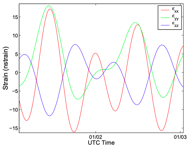
Figure 1: Figure from Doan, Brodsky, Prioul and Signer showing strain-tensor components for a particular place and time window.
I think it likely that direct measurements of strain would be very useful when modelling real situations. This could be accomplished using fibre optics (Becker and Coleman, 2019).
Earth tides: a MOOSE model
Now consider a fully-saturated, confined aquifer. PorousFlow may be used to simulate the porepressure response to these applied strains.
# A confined aquifer is fully saturated with water
# Earth tides apply strain to the aquifer and the resulting porepressure changes are recorded
#
# To replicate standard poroelasticity exactly:
# (1) the PorousFlowBasicTHM Action is used;
# (2) multiply_by_density = false;
# (3) PorousFlowConstantBiotModulus is used
[Mesh]
  type = GeneratedMesh
  dim = 3
  nx = 1
  ny = 1
  nz = 1
  xmin = 0
  xmax = 1
  ymin = 0
  ymax = 1
  zmin = 0
  zmax = 1
[]

[GlobalParams]
  displacements = 'disp_x disp_y disp_z'
  PorousFlowDictator = dictator
  block = 0
  biot_coefficient = 0.6
  multiply_by_density = false
[]

[Variables]
  [disp_x]
  []
  [disp_y]
  []
  [disp_z]
  []
  [porepressure]
  []
[]

[BCs]
  [strain_x]
    type = FunctionDirichletBC
    variable = disp_x
    function = earth_tide_x
    boundary = 'left right'
  []
  [strain_y]
    type = FunctionDirichletBC
    variable = disp_y
    function = earth_tide_y
    boundary = 'bottom top'
  []
  [strain_z]
    type = FunctionDirichletBC
    variable = disp_z
    function = earth_tide_z
    boundary = 'back front'
  []
[]

[Functions]
  [earth_tide_x]
    type = ParsedFunction
    value = 'x*1E-8*(5*cos(t*2*pi) + 2*cos((t-0.5)*2*pi) + 1*cos((t+0.3)*0.5*pi))'
  []
  [earth_tide_y]
    type = ParsedFunction
    value = 'y*1E-8*(7*cos(t*2*pi) + 4*cos((t-0.3)*2*pi) + 7*cos((t+0.6)*0.5*pi))'
  []
  [earth_tide_z]
    type = ParsedFunction
    value = 'z*1E-8*(7*cos((t-0.5)*2*pi) + 4*cos((t-0.8)*2*pi) + 7*cos((t+0.1)*4*pi))'
  []
[]

[Modules]
  [FluidProperties]
    [the_simple_fluid]
      type = SimpleFluidProperties
      bulk_modulus = 2E9
    []
  []
[]

[PorousFlowBasicTHM]
  coupling_type = HydroMechanical
  displacements = 'disp_x disp_y disp_z'
  porepressure = porepressure
  gravity = '0 0 0'
  fp = the_simple_fluid
[]

[Materials]
  [elasticity_tensor]
    type = ComputeIsotropicElasticityTensor
    bulk_modulus = 10.0E9 # drained bulk modulus
    poissons_ratio = 0.25
  []
  [strain]
    type = ComputeSmallStrain
  []
  [stress]
    type = ComputeLinearElasticStress
  []
  [porosity]
    type = PorousFlowPorosityConst # only the initial value of this is ever used
    porosity = 0.1
  []
  [biot_modulus]
    type = PorousFlowConstantBiotModulus
    solid_bulk_compliance = 1E-10
    fluid_bulk_modulus = 2E9
  []
  [permeability]
    type = PorousFlowPermeabilityConst
    permeability = '1E-12 0 0   0 1E-12 0   0 0 1E-12'
  []
[]

[Postprocessors]
  [pp]
    type = PointValue
    point = '0.5 0.5 0.5'
    variable = porepressure
  []
[]

[Preconditioning]
  [smp]
    type = SMP
    full = true
  []
[]

[Executioner]
  type = Transient
  solve_type = Newton
  dt = 0.01
  end_time = 2
[]

[Outputs]
  console = true
  csv = true
[]
In this setup, the porepressure, , is controlled by the undrained bulk modulus and the Skempton coefficient where the repeated index indicates summation (). Substituting numbers yields (1)
For a time-independent strain field, PorousFlow reproduces Eq. (1) exactly. For a synthetically-generated time-dependent strain field, the porepressure changes accordingly, as shown in Figure 2.
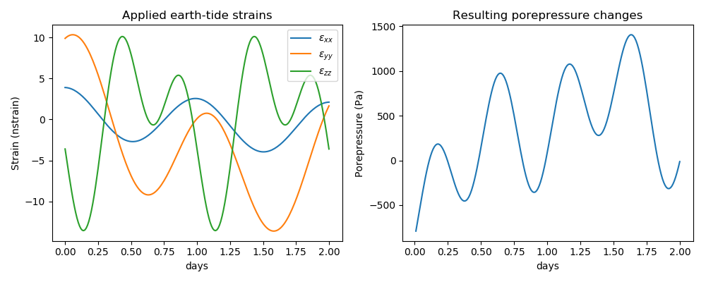
Figure 2: Example time-dependent strain field, and corresponding porepressure change in a confined aquifer.
Earth tides: varying
Realistic material properties and strain magnitudes have been used in the above MOOSE example, and the changes in porepressure are around kPa. This is much more than the change due to small variations in the gravitational acceleration, which would be around . For liquid water of density kg.m at the bottom of a water column of height m, a change of m.s, results in a porepressure change of around Pa. For a shallower case with m, the porepressure change is even smaller (Pa).
At the time of writing (August 2019) the gravitational acceleration vector in MOOSE and PorousFlow cannot be time-dependent. This is not a difficult addition to make (using AuxVariables) but the arguments in the preceding paragraph suggest it is unnecessary.
Currently, I'm wondering about the impact of heterogeneity on these arguments. A more realistic MOOSE model would include different lithologies. The boundary conditions on the displacement Variables could simply result from the earth strains (as in the above PorousFlow example). Heterogeneity would then mean the strain was not uniform throughout the model. Does this mean that changes in become more important?
Barometric and oceanic loading
Conceptually, barometric and oceanic loading are similar as they both serve to change porepressure and load the porous matrix. A numerical model must consider whether boreholes are open to the atmosphere, or sealed, and whether the aquifers are confined or unconfined. Interestingly, Doan et al. (December 20, 2006) report that ocean tides can impact porous flows km inland ( lag in the Pinon Flat Observatory). On the other hand, CSIRO has observed no impact of ocean tides only km inland.
Boundary conditions for barometric and oceanic loading
Conceptually, external fluids such as the atmosphere, ocean, borehole fluids or hydraulic-fracturing fluids mechanically load the porous matrix. Mathematically, the external fluid pressure acts as an applied total stress at the boundary of the porous matrix (for instance, see Detournay and Cheng (1991)).
Conceptually, the porepressure responds instantly to the external fluid pressure. Mathematically, the porepressure (of the relevant phase) at the boundary of the porous matrix is equal to the external fluid pressure.
BCs: total stress
The total stress, , at the interface of the porous-matrix and the atmosphere must be equal to the atmospheric pressure, : (2) The same holds for the oceanic pressure. Here labels the normal direction and the negative sign comes because corresponds to a compressive stress, which is . This is boundary condition arises because the atmosphere or ocean is physically pushing on the porous matrix.
BCs: porepressure
The porepressure, , at the interface of the porous-matrix and the atmosphere must be equal to the atmospheric pressure: (3) In a multi-phase scenario, this equation would read .
Combining Eq. (2) and Eq. (3) in the single-phase case means the effective stress at the interface is The Biot coefficient, , can be interpreted as an effective way of accounting for pores that aren't filled with water. When all the porespace is filled with water, and the above equation reads , so an increase in atmospheric pressure produces zero strain: the porewater pushes back on the porous skeleton with the same magnitude as the atmosphere. When , the above equation means that an increase in atmospheric pressure results in a compression: the porewater doesn't fill tne entire porespace so isn't as effective at "pushing back" and can't match the load of the atmospheric pressure.
BCs: within a water-filled borehole
If a borehole is open, then the bottomhole pressure varies linearly with the atmospheric pressure: .
For a sealed section of a well, the borehole pressure is the same as the porepressure within the adjacent rock.
Atmospheric loading on a fully-confined, fully-saturated aquifer: barometric efficiency
Here, "fully confined" means the aquifer is completely enclosed by aquitards of zero permeability. Imagine the fully-saturated aquifer is horizontal, has infinite extent and a uniform thickness. It is undrained for its water cannot escape. This example is artificially idealised: sections below explain how to extend this analysis to partially-confined or unconfined aquifers.
Because of the fully-confined nature (zero-permeability aquitards), any porepressure changes at the topography are not felt in the aquifer. Therefore, Eq. (2) applied to the aquifer's top is the only non-trivial BC. As for the other BCs: it is assumed that aquifer's other boundaries are fixed, and all boundaries are impermeable to water. The input file is:
# A fully-confined aquifer is fully saturated with water
# Barometric loading is applied to the aquifer.
# Because the aquifer is assumed to be sandwiched between
# impermeable aquitards, the barometric pressure is not felt
# directly by the porepressure.  Instead, the porepressure changes
# only because the barometric loading applies a total stress to
# the top surface of the aquifer.
#
# To replicate standard poroelasticity exactly:
# (1) the PorousFlowBasicTHM Action is used;
# (2) multiply_by_density = false;
# (3) PorousFlowConstantBiotModulus is used
[Mesh]
  type = GeneratedMesh
  dim = 3
  nx = 1
  ny = 1
  nz = 1
  xmin = 0
  xmax = 1
  ymin = 0
  ymax = 1
  zmin = 0
  zmax = 1
[]

[GlobalParams]
  displacements = 'disp_x disp_y disp_z'
  PorousFlowDictator = dictator
  block = 0
  biot_coefficient = 0.6
  multiply_by_density = false
[]

[Variables]
  [disp_x]
  []
  [disp_y]
  []
  [disp_z]
  []
  [porepressure]
  []
[]

[BCs]
  [fix_x]
    type = DirichletBC
    variable = disp_x
    value = 0.0
    boundary = 'left right'
  []
  [fix_y]
    type = DirichletBC
    variable = disp_y
    value = 0.0
    boundary = 'bottom top'
  []
  [fix_z_bottom]
    type = DirichletBC
    variable = disp_z
    value = 0.0
    boundary = back
  []
  [barometric_loading]
    type = FunctionNeumannBC
    variable = disp_z
    function = -1000.0 # atmospheric pressure increase of 1kPa
    boundary = front
  []
[]

[Modules]
  [FluidProperties]
    [the_simple_fluid]
      type = SimpleFluidProperties
      bulk_modulus = 2E9
    []
  []
[]

[PorousFlowBasicTHM]
  coupling_type = HydroMechanical
  displacements = 'disp_x disp_y disp_z'
  porepressure = porepressure
  gravity = '0 0 0'
  fp = the_simple_fluid
[]

[Materials]
  [elasticity_tensor]
    type = ComputeIsotropicElasticityTensor
    bulk_modulus = 10.0E9 # drained bulk modulus
    poissons_ratio = 0.25
  []
  [strain]
    type = ComputeSmallStrain
  []
  [stress]
    type = ComputeLinearElasticStress
  []
  [porosity]
    type = PorousFlowPorosityConst # only the initial value of this is ever used
    porosity = 0.1
  []
  [biot_modulus]
    type = PorousFlowConstantBiotModulus
    solid_bulk_compliance = 1E-10
    fluid_bulk_modulus = 2E9
  []
  [permeability]
    type = PorousFlowPermeabilityConst
    permeability = '1E-12 0 0   0 1E-12 0   0 0 1E-12'
  []
[]

[Postprocessors]
  [pp]
    type = PointValue
    point = '0.5 0.5 0.5'
    variable = porepressure
  []
[]

[Preconditioning]
  [smp]
    type = SMP
    full = true
  []
[]

[Executioner]
  type = Transient
  solve_type = Newton
  dt = 1
  end_time = 1
[]

[Outputs]
  console = true
  csv = true
[]
Doan et al. (December 20, 2006) introduce this example, and state the porepressure response in their Equation (3.1): Here is called the barometric efficiency. For the parameters listed in Table 1 it is . The MOOSE model reproduces this exactly.
Atmospheric loading on an unconfined, fully-saturated aquifer
Changes of atmospheric pressure directly impact the porepressure within the rock, as well as acting on the rock skeleton. Consider the model shown in Figure 3.

Figure 3: Geometry of the unconfined, fully-saturated aquifer.
Use the following assumptions.
The atmospheric pressure varies as kPa.
The boundaries are impermeable except the top boundary
Only vertical displacement is allowed
The barometric loading acts on the total stress at the model's top, as in Eq. (2)
The MOOSE input file is:
# A 10m x 10m "column" of height 100m is subjected to cyclic pressure at its top
# Assumptions:
# the boundaries are impermeable, except the top boundary
# only vertical displacement is allowed
# the atmospheric pressure sets the total stress at the top of the model
[Mesh]
  type = GeneratedMesh
  dim = 3
  nx = 1
  ny = 1
  nz = 10
  xmin = 0
  xmax = 10
  ymin = 0
  ymax = 10
  zmin = -100
  zmax = 0
[]

[GlobalParams]
  displacements = 'disp_x disp_y disp_z'
  PorousFlowDictator = dictator
  block = 0
  biot_coefficient = 0.6
  multiply_by_density = false
[]

[Variables]
  [disp_x]
  []
  [disp_y]
  []
  [disp_z]
  []
  [porepressure]
    scaling = 1E11
  []
[]

[ICs]
  [porepressure]
    type = FunctionIC
    variable = porepressure
    function = '-10000*z'  # approximately correct
  []
[]

[Functions]
  [ini_stress_zz]
    type = ParsedFunction
    value = '(25000 - 0.6*10000)*z' # remember this is effective stress
  []
  [cyclic_porepressure]
    type = ParsedFunction
    value = 'if(t>0,5000 * sin(2 * pi * t / 3600.0 / 24.0),0)'
  []
  [neg_cyclic_porepressure]
    type = ParsedFunction
    value = '-if(t>0,5000 * sin(2 * pi * t / 3600.0 / 24.0),0)'
  []
[]

[BCs]
  # zmin is called 'back'
  # zmax is called 'front'
  # ymin is called 'bottom'
  # ymax is called 'top'
  # xmin is called 'left'
  # xmax is called 'right'
  [no_x_disp]
    type = DirichletBC
    variable = disp_x
    value = 0
    boundary = 'bottom top' # because of 1-element meshing, this fixes u_x=0 everywhere
  []
  [no_y_disp]
    type = DirichletBC
    variable = disp_y
    value = 0
    boundary = 'bottom top' # because of 1-element meshing, this fixes u_y=0 everywhere
  []
  [no_z_disp_at_bottom]
    type = DirichletBC
    variable = disp_z
    value = 0
    boundary = back
  []
  [pp]
    type = FunctionDirichletBC
    variable = porepressure
    function = cyclic_porepressure
    boundary = front
  []
  [total_stress_at_top]
    type = FunctionNeumannBC
    variable = disp_z
    function = neg_cyclic_porepressure
    boundary = front
  []
[]

[Modules]
  [FluidProperties]
    [the_simple_fluid]
      type = SimpleFluidProperties
      thermal_expansion = 0.0
      bulk_modulus = 2E9
      viscosity = 1E-3
      density0 = 1000.0
    []
  []
[]

[PorousFlowBasicTHM]
  coupling_type = HydroMechanical
  displacements = 'disp_x disp_y disp_z'
  porepressure = porepressure
  gravity = '0 0 -10'
  fp = the_simple_fluid
[]

[Materials]
  [elasticity_tensor]
    type = ComputeIsotropicElasticityTensor
    bulk_modulus = 10.0E9 # drained bulk modulus
    poissons_ratio = 0.25
  []
  [strain]
    type = ComputeSmallStrain
    eigenstrain_names = ini_stress
  []
  [stress]
    type = ComputeLinearElasticStress
  []
  [ini_stress]
    type = ComputeEigenstrainFromInitialStress
    initial_stress = '0 0 0  0 0 0  0 0 ini_stress_zz'
    eigenstrain_name = ini_stress
  []
  [porosity]
    type = PorousFlowPorosityConst # only the initial value of this is ever used
    porosity = 0.1
  []
  [biot_modulus]
    type = PorousFlowConstantBiotModulus
    solid_bulk_compliance = 1E-10
    fluid_bulk_modulus = 2E9
  []
  [permeability]
    type = PorousFlowPermeabilityConst
    permeability = '1E-12 0 0   0 1E-12 0   0 0 1E-14'
  []
  [density]
    type = GenericConstantMaterial
    prop_names = density
    prop_values = 2500.0
  []
[]

[Postprocessors]
  [p0]
    type = PointValue
    outputs = csv
    point = '0 0 0'
    variable = porepressure
  []
  [uz0]
    type = PointValue
    outputs = csv
    point = '0 0 0'
    variable = disp_z
  []
  [p100]
    type = PointValue
    outputs = csv
    point = '0 0 -100'
    variable = porepressure
  []
[]

[Preconditioning]
  [andy]
    type = SMP
    full = true
  []
[]

[Executioner]
  type = Transient
  solve_type = Newton
  start_time = -3600 # so postprocessors get recorded correctly at t=0
  dt = 3600
  end_time = 360000
  nl_abs_tol = 5E-7
  nl_rel_tol = 1E-10
[]

[Outputs]
  csv = true
[]
The results in Figure 4 show that, in this model, a realistic barometric fluctuation of kPa produces a vertical displacement of about mm and that the porepressure at depth experiences a phase lag and amplitude reduction, as expected. Figure 4 shows the first few sinusoidal periods. After about 5 periods, transient responses have more-or-less disappeared.
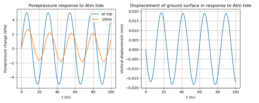
Figure 4: Response of the fully-saturated, unconfined aquifer to cyclic barometric pressure. The first few sinusoidal periods are shown: after this time transient behaviour has mostly disappeared.
Atmospheric loading on an unconfined, fully-saturated aquifer containing an open borehole
This model includes a borehole. The borehole is assumed to be cased, except for the very bottom section at 100m depth. Therefore, groundwater seeps into the borehole and rises up the hole until it reaches the ground level (where porepressure is zero). Furthermore, it is assumed in this example that the borehole is always full of water (for example, as water is pushed into the rock skeleton it is magically replenished). Similarly it is assumed the rock skeleton is always fully saturated. The setup is shown in Figure 5 and the results are shown in Figure 6. Figure 6 shows the first few sinusoidal periods. After about 5 periods, transient responses have more-or-less disappeared.
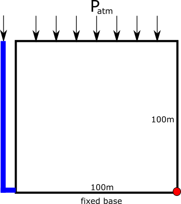
Figure 5: Geometry of the unconfined, fully-saturated aquifer containing a borehole that is cased to 100m. The porepressure observation point is shown in red.
# A 100m x 10m "slab" of height 100m is subjected to cyclic pressure at its top
# Assumptions:
# the boundaries are impermeable, except the top boundary
# only vertical displacement is allowed
# the atmospheric pressure sets the total stress at the top of the model
# at the slab left-hand side there is a borehole that taps into the base of the slab.
[Mesh]
  [the_mesh]
    type = GeneratedMeshGenerator
    dim = 3
    nx = 10
    ny = 1
    nz = 10
    xmin = 0
    xmax = 100
    ymin = -5
    ymax = 5
    zmin = -100
    zmax = 0
  []
  [bh_back]
    type = ExtraNodesetGenerator
    coord = '0 -5 -100'
    input = the_mesh
    new_boundary = 11
  []
[]

[GlobalParams]
  displacements = 'disp_x disp_y disp_z'
  PorousFlowDictator = dictator
  block = 0
  biot_coefficient = 0.6
  multiply_by_density = false
[]

[Variables]
  [disp_x]
  []
  [disp_y]
  []
  [disp_z]
  []
  [porepressure]
    scaling = 1E11
  []
[]

[ICs]
  [porepressure]
    type = FunctionIC
    variable = porepressure
    function = '-10000*z'  # this is only approximately correct
  []
[]

[Functions]
  [ini_stress_zz]
    type = ParsedFunction
    value = '(25000 - 0.6*10000)*z' # remember this is effective stress
  []
  [cyclic_porepressure]
    type = ParsedFunction
    value = 'if(t>0,5000 * sin(2 * pi * t / 3600.0 / 24.0),0)'
  []
  [cyclic_porepressure_at_depth]
    type = ParsedFunction
    value = '-10000*z + if(t>0,5000 * sin(2 * pi * t / 3600.0 / 24.0),0)'
  []
  [neg_cyclic_porepressure]
    type = ParsedFunction
    value = '-if(t>0,5000 * sin(2 * pi * t / 3600.0 / 24.0),0)'
  []
[]

[BCs]
  # zmin is called 'back'
  # zmax is called 'front'
  # ymin is called 'bottom'
  # ymax is called 'top'
  # xmin is called 'left'
  # xmax is called 'right'
  [no_x_disp]
    type = DirichletBC
    variable = disp_x
    value = 0
    boundary = 'bottom top' # because of 1-element meshing, this fixes u_x=0 everywhere
  []
  [no_y_disp]
    type = DirichletBC
    variable = disp_y
    value = 0
    boundary = 'bottom top' # because of 1-element meshing, this fixes u_y=0 everywhere
  []
  [no_z_disp_at_bottom]
    type = DirichletBC
    variable = disp_z
    value = 0
    boundary = back
  []
  [pp]
    type = FunctionDirichletBC
    variable = porepressure
    function = cyclic_porepressure
    boundary = front
  []
  [pp_downhole]
    type = FunctionDirichletBC
    variable = porepressure
    function = cyclic_porepressure_at_depth
    boundary = 11
  []
  [total_stress_at_top]
    type = FunctionNeumannBC
    variable = disp_z
    function = neg_cyclic_porepressure
    boundary = front
  []
[]

[Modules]
  [FluidProperties]
    [the_simple_fluid]
      type = SimpleFluidProperties
      thermal_expansion = 0.0
      bulk_modulus = 2E9
      viscosity = 1E-3
      density0 = 1000.0
    []
  []
[]

[PorousFlowBasicTHM]
  coupling_type = HydroMechanical
  displacements = 'disp_x disp_y disp_z'
  porepressure = porepressure
  gravity = '0 0 -10'
  fp = the_simple_fluid
[]

[Materials]
  [elasticity_tensor]
    type = ComputeIsotropicElasticityTensor
    bulk_modulus = 10.0E9 # drained bulk modulus
    poissons_ratio = 0.25
  []
  [strain]
    type = ComputeSmallStrain
    eigenstrain_names = ini_stress
  []
  [stress]
    type = ComputeLinearElasticStress
  []
  [ini_stress]
    type = ComputeEigenstrainFromInitialStress
    initial_stress = '0 0 0  0 0 0  0 0 ini_stress_zz'
    eigenstrain_name = ini_stress
  []
  [porosity]
    type = PorousFlowPorosityConst # only the initial value of this is ever used
    porosity = 0.1
  []
  [biot_modulus]
    type = PorousFlowConstantBiotModulus
    solid_bulk_compliance = 1E-10
    fluid_bulk_modulus = 2E9
  []
  [permeability]
    type = PorousFlowPermeabilityConst
    permeability = '1E-14 0 0   0 1E-14 0   0 0 1E-14'
  []
  [density]
    type = GenericConstantMaterial
    prop_names = density
    prop_values = 2500.0
  []
[]

[Postprocessors]
  [p0_0]
    type = PointValue
    outputs = csv
    point = '0 0 0'
    variable = porepressure
  []
  [p100_0]
    type = PointValue
    outputs = csv
    point = '100 0 0'
    variable = porepressure
  []
  [p0_100]
    type = PointValue
    outputs = csv
    point = '0 0 -100'
    variable = porepressure
  []
  [p100_100]
    type = PointValue
    outputs = csv
    point = '100 0 -100'
    variable = porepressure
  []
  [uz0]
    type = PointValue
    outputs = csv
    point = '0 0 0'
    variable = disp_z
  []
  [uz100]
    type = PointValue
    outputs = csv
    point = '100 0 0'
    variable = disp_z
  []
[]

[Preconditioning]
  [andy]
    type = SMP
    full = true
  []
[]

[Executioner]
  type = Transient
  solve_type = Newton
  start_time = -3600
  dt = 3600
  end_time = 172800
  nl_rel_tol = 1E-10
  nl_abs_tol = 1E-5
[]

[Outputs]
  print_linear_residuals = false
  csv = true
[]
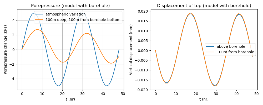
Figure 6: Response of the fully-saturated, unconfined aquifer containing an open borehole to cyclic barometric pressure. The first few sinusoidal periods are shown: after this time transient behaviour has mostly disappeared.
Bibliography
References
- Matthew W. Becker and Thomas I. Coleman.
Distributed acoustic sensing of strain at earth tide frequencies.
Sensors, 19:1–9, 2019.
doi:10.3390/s19091975.[BibTeX]
- E. Detournay and A. Cheng.
“Fundamentals of poroelasticity,” Chapter 5 in Comprehensive Rock Engineering: Principles, Practice and Projects, Vol II, Analysis and Design Method. Also available online.
Pergamon Press, New York, 1993.[BibTeX]
- Emmanuel Detournay and Alexander H.-D. Cheng.
Plane strain analysis of a stationary hydraulic fracture in a poroelastic medium.
International Journal of Solids and Structures, 27(13):1645–1662, 1991.
doi:10.1016/0020-7683(91)90067-P.[BibTeX]
- Mai-Linh Doan, Emily E. Brodsky, Romain Prioul, and Claude Signer.
Tidal analysis of borehole pressure: a tutorial.
December 20, 2006.
URL: https://pdfs.semanticscholar.org/3870/124883b5621d35fae814b1cd0f050f642bfc.pdf.[BibTeX]
- Kare Langaas, Knut I. Nilsen, and Svein M. Skjaeveland.
Tidal Pressure Response and Surveillance of Water Encroachment.
Society of Petroleum Engineers, Reservoir Evaluation and Engineering, 9:335–344, 2006.
doi:10.2118/95763-PA.[BibTeX]
- Gabriel C. Rau.
Pygtide.
2018.
hydrogeoscience/pygtide: PyGTide v0.2 (Version v0.2). Zenodo.
URL: https://github.com/hydrogeoscience/pygtide, doi:10.5281/zenodo.1346664.[BibTeX]
- Kozo Sato.
Monitoring the underground migration of sequestered carbon dioxide using Earth tides.
Energy Conversion and Management, 47:2414–2423, 2006.
doi:10.1016/j.enconman.2005.11.005.[BibTeX]
- Kozo Sato and Roland N. Horne.
Time-lapse analysis of pressure transients due to ocean tides for estimating CO$_2$ saturation changes.
International Journal of Greenhouse Gas Control, 18:160–167, 2018.
doi:10.1016/j.ijggc.2018.08.005.[BibTeX]
- Herbert F. Wang.
Theory of Linear Poroelasticity with Applications to Geomechanics and Hydrogeology.
Princeton University Press, 2000.
ISBN 9781400885688.[BibTeX]