Cold CO injection into an elastic reservoir - a multi-phase THM problem
Andy Wilkins, Chris Green, Jonathan Ennis-King
Two papers of LaForce et al. (LaForce et al., 2014a; LaForce et al., 2014b) derive semi-analytical solutions of a 2-phase THM problem involving injection of a cold fluid into a warmer, elastic reservoir depicted in Figure 1. In this page, their solution will be replicated in MOOSE. The nomenclature used here is described in a separate page.
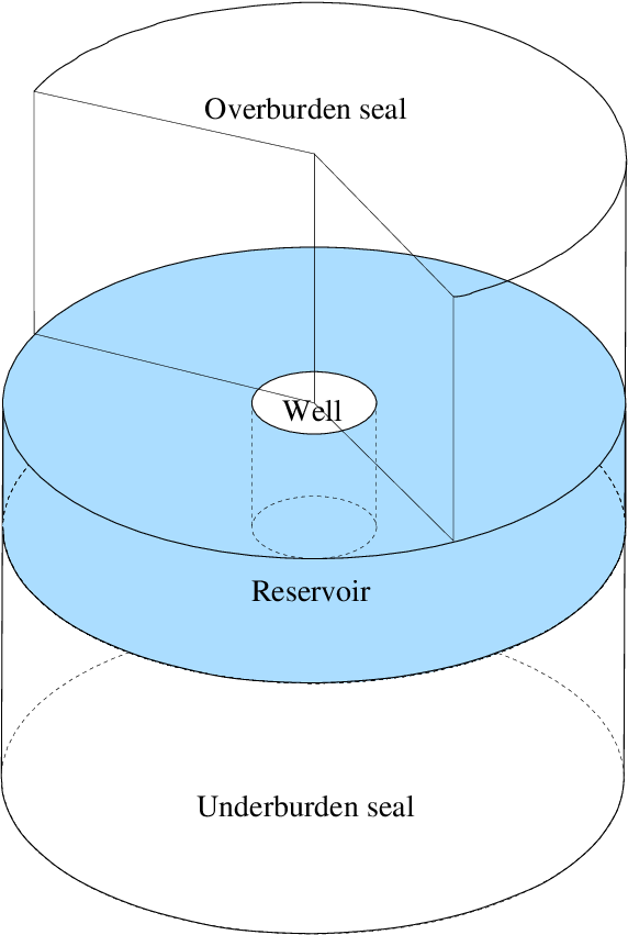
Figure 1: The geometrical setup used in the papers of LaForce et al.
LaForce et al. consider a cylindrically-symmetric model, as depicted in Figure 1, with radial coordinate labelled by and axial coordinate . A permeable reservoir is sandwiched between two impermeable seals. The reservoir and seals are oriented horizontally (normal to ). The reservoir is initially fully water saturated.
A vertical wellbore intersects the reservoir and injects CO into it at a constant rate. The CO is colder than the initial reservoir temperature. The injected fluid advects through the reservoir (but not through the impermeable seals). Heat (or cold) advects with the fluid, slowly cooling the reservoir, and conducting into the surrounding seals.
The PorousFlow input file and associated scripts that generate the analytic solutions are here. The input file describes an axially symmetric situation:
[Mesh]
  type = GeneratedMesh
  dim = 2
  nx = 2000
  bias_x = 1.003
  xmin = 0.1
  xmax = 5000
  ny = 1
  ymin = 0
  ymax = 11
[]
[Problem]
  coord_type = RZ
[]
Equations and assumptions
To derive the semi-analytical solutions, LaForce et al. employ the assumptions stated below.
Fluid flow: mass
In PorousFlow, the mass of species per volume of rock is written as a sum over all phases present in the system: (1) LaForce et al. make the following assumptions
The porosity, , is constant. It is independent of time, fluid pressure, temperature and volumetric expansion. However, it is dependent on rock type.
  [porosity_reservoir]
    type = PorousFlowPorosityConst
    porosity = 0.2
  []
There are two phases, liquid and gas. Hence .
The liquid is water and the gas is CO. Hence . The water component exists only in the liquid phase and the CO component exists only in the gas phase. Hence , , and .
  [massfrac_ph0_sp0]
    initial_condition = 1 # all H20 in phase=0
  []
  [massfrac_ph1_sp0]
    initial_condition = 0 # no H2O in phase=1
  []
The density of each phase is constant. This is in order to simplify the fluid equations, which eventually reduce to a well-studied form that models advection of a saturation shock front. However, in order to derive solutions for the pressure distribution, LaForce et al. assume a small fluid compressibility, which is the same for each phase. To satisfy both the incompressibility and small compressibility requirements, the MOOSE model uses a fluid bulk modulus that is larger than any porepressures.
There is no desorbed fluid.
With these assumptions, the mass formula becomes
The PorousFlow input file uses the porepressure of water and the gas saturation as its primary nonlinear variables describing fluid flow:
  [pwater]
    initial_condition = 18.3e6
  []
  [sgas]
    initial_condition = 0.0
  []
Fluid flow: flux
In PorousFlow, the flux is a sum of advective flux and diffusive-and-dispersive flux: (2) Advective flux is governed by Darcy's law: (3) Diffusion and dispersion are proportional to the gradient of : (4)
LaForce et al. make the following assumptions
The permeability tensor is diagonal and constant (independent of fluid pressure, temperature and rock stress and strain). Its and components are equal, and its component is zero. It is dependent on rock type. Since the PorousFlow input file is setup in 2D RZ coordinates, the radial permeability enters the first "slot", the component appears in the central slot, and all other components are zero in this situation
  [permeability_reservoir]
    type = PorousFlowPermeabilityConst
    permeability = '2e-12 0 0  0 0 0  0 0 0'
  []
There is a constant and nonzero residual water saturation and constant and nonzero residual CO saturation .
The relative permeability functions are functions of the effective saturation and the functions are (17)
  [relperm_liquid]
    type = PorousFlowRelativePermeabilityCorey
    n = 4
    phase = 0
    s_res = 0.200
    sum_s_res = 0.405
  []
  [relperm_gas]
    type = PorousFlowRelativePermeabilityBC
    phase = 1
    s_res = 0.205
    sum_s_res = 0.405
    nw_phase = true
    lambda = 2
  []
The viscosity is a function of temperature only. LaForce et al. use a particular function of temperature that is not included in PorousFlow. Therefore, here we shall use constant viscosity for each phase that is equal to the average viscosity quoted in LaForce et al., and use LaForce et al.'s solution based on that constant viscosity. This results in only very tiny modifications to LaForce's solutions which would be difficult to see in the finite-resolution of the MOOSE model anyway.
There is no capillarity. Therefore . Define .
  [pc]
    type = PorousFlowCapillaryPressureConst
    pc = 0
There is no gravity.
There is no diffusion and dispersion (which is implicitly implied by the assumptions on ).
With these assumptions, the fluid fluxes are
Fluid flow: mass conservation
In PorousFlow, mass conservation for fluid species is described by the continuity equation (5)
LaForce et al. make the following assumptions:
The term is ignored.
There is no radioactive decay, .
Sources and sinks only occur on the boundary, so except for on the boundary.
Therefore, the fluid-flow Kernels are
  [mass_water_dot]
    type = PorousFlowMassTimeDerivative
    fluid_component = 0
    variable = pwater
  []
  [flux_water]
    type = PorousFlowAdvectiveFlux
    fluid_component = 0
    use_displaced_mesh = false
    variable = pwater
  []
  [mass_co2_dot]
    type = PorousFlowMassTimeDerivative
    fluid_component = 1
    variable = sgas
  []
  [flux_co2]
    type = PorousFlowAdvectiveFlux
    fluid_component = 1
    use_displaced_mesh = false
    variable = sgas
  []
Fluid flow: summary
With all the assumptions so far, the mass conservation equations read The sum of these yields the total flow rate: This total flow rate is dependent on time (controlled by the boundary conditions) but satisfies .
For later use, define the fractional flows (6)
Heat flow: heat energy
In PorousFlow, the heat energy per unit volume is (7)
LaForce et al. make the following assumptions
The rock grain density, , is constant.
The specific heat capacity of the rock grains, , is constant.
  [internal_energy_reservoir]
    type = PorousFlowMatrixInternalEnergy
    specific_heat_capacity = 1100
    density = 2350.0
  []
The internal energy of the liquid phase is , where is constant and independent of all other parameters in the system.
The internal energy of the gas phase is , where is constant and independent of all other parameters of the system.
With these assumptions the heat energy density is
Heat flow: flux
In PorousFlow, the heat flux is a sum of heat conduction and convection with the fluid: (8)
LaForce et al. make the following assumptions
The only non-zero component of the thermal conductivity is the component. It varies with water saturation The coefficients and are independent of time, fluid pressure, temperature and mechanical deformation, but they are dependent on rock type.
  [thermal_conductivity_reservoir]
    type = PorousFlowThermalConductivityIdeal
    dry_thermal_conductivity = '0 0 0  0 1.320 0  0 0 0'
    wet_thermal_conductivity = '0 0 0  0 3.083 0  0 0 0'
  []
The enthalpy of the liquid phase is .
The enthalpy of the gas phase is .
With the assumptions made so far where the fractional flows of Eq. (6) have been employed.
Heat flow: energy conservation
In PorousFlow, energy conservation for heat is described by the continuity equation (9)
LaForce et al. make the following assumptions
There is no plastic heating.
There are no heat sources, save for on the boundary.
Heat flow: summary
With the assumptions made so far, the heat equation reads (10) where the following two variables, and have been defined: (11) Eq. (10) and Eq. (11) are exactly Eq. (A1) in LaForce et al. (2014a).
During the course of their analysis, LaForce et al. replace the diffusive term, with a Lauwerier heat-loss expression: (12) In terms of LaForce et al.'s variables, the new heat-loss coefficient is (13) This is a particularly nice simplification because it means that the overburden and underburden don't need to be considered any further in the analysis. It does mean, however, that the mechanical effects of these surrounding rocks on the aquifer are not modelled by LaForce et al.
Therefore, the heat-flow Kernels are
  [energy_dot]
    type = PorousFlowEnergyTimeDerivative
    variable = temp
  []
  [advection]
    type = PorousFlowHeatAdvection
    use_displaced_mesh = false
    variable = temp
  []
  [conduction]
    type = PorousFlowExponentialDecay
    use_displaced_mesh = false
    variable = temp
    reference = 358
    rate = rate
  []
along with the rate of heat loss:
[Functions]
  [decay_rate]
    # Eqn(26) of the first paper of LaForce et al.
    # Ka * (rho C)_a = 10056886.914
    # h = 11
    type = ParsedFunction
    value = 'sqrt(10056886.914/t)/11.0'
  []
[]
Solid mechanics
Denote the effective stress tensor by . In PorousFlow it is defined by (14)
LaForce et al. assume
The Biot coefficient, , is constant and independent of all other parameters in the theory.
The effective fluid pressure is
  [eff_fluid_pressure]
    type = PorousFlowEffectiveFluidPressure
  []
In PorousFlow, the solid-mechanical constitutive law reads (15)
LaForce et al. assume
The drained elasticity tensor, , is isotropic, constant and independent of all other parameters in the theory.
  [elasticity_tensor]
    type = ComputeIsotropicElasticityTensor
    shear_modulus = 6.0E9
    poissons_ratio = 0.2
  []
There is no plasticity.
The drained thermal expansion coefficient, , is constant and independent of all other parameters in the theory.
  [strain]
    type = ComputeAxisymmetricRZSmallStrain
    eigenstrain_names = 'thermal_contribution ini_stress'
  []
  [ini_strain]
    type = ComputeEigenstrainFromInitialStress
    initial_stress = '-12.8E6 0 0  0 -51.3E6 0  0 0 -12.8E6'
    eigenstrain_name = ini_stress
  []
  [thermal_contribution]
    type = ComputeThermalExpansionEigenstrain
    temperature = temp
    stress_free_temperature = 358
    thermal_expansion_coeff = 5E-6
    eigenstrain_name = thermal_contribution
  []
  [stress]
    type = ComputeLinearElasticStress
  []
In PorousFlow, conservation of momentum reads (16)
LaForce et al. assume
The acceleration of the solid skeleton, , is zero.
There are no body forces, , except for on the boundary.
Further assumptions and implications
LaForce et al. make the following assumptions:
There is no displacement in the direction, . The solid-mechanics
Kernelsare therefore
  [grad_stress_r]
    type = StressDivergenceRZTensors
    temperature = temp
    eigenstrain_names = thermal_contribution
    variable = disp_r
    use_displaced_mesh = false
    component = 0
The reservoir is free to contract and expand radially without being hindered by the impermeable seals.
There is no dependence on the axial coordinates, , because of the use of the Lauwerier heat-loss model (Eq. (12)) that simulates axial heat conduction. Therefore, all independent variables — the water saturation , fluid porepressure , temperature , and radial displacement — are dependent on radius only.
The Variables used in the PorousFlow input file are:
[Variables]
  [pwater]
    initial_condition = 18.3e6
  []
  [sgas]
    initial_condition = 0.0
  []
  [temp]
    initial_condition = 358
  []
  [disp_r]
  []
[]
Parameter values and initial conditions
Table 1: Parameters and their numerical values used in the benchmark against LaForce et al.
| Symbol | Value | Physical description |
|---|---|---|
| 1.0 | Biot coefficient for reservoir and seals | |
| K | Drained linear thermal expansion coefficient of the reservoir and seals | |
| 1100J.kg.K | Specific heat capacity of reservoir rock grains | |
| 828.9J.kg.K | Specific heat capacity of seal rock grains | |
| 2920.5J.kg.K | Specific heat capacity of water | |
| 4149J.kg.K | Specific heat capacity of water | |
| 0.2 | Porosity of reservoir | |
| 0.02 | Porosity of seals | |
| 6GPa | Shear modulus of the reservoir and seals | |
| 11m | Vertical height of the reservoir | |
| Tonne.year | Injection rate of CO. | |
| 8GPa | Drained bulk modulus of the reservoir and seals | |
| GPa | Bulk density of water | |
| GPa | Bulk density of CO | |
| m | horizontal permeability components of the reservoir (there is zero vertical permeability) | |
| 0 | permeability of seal | |
| 1.32J.s.m.K | Vertical thermal conductivity of reservoir at zero water saturation | |
| 3.083J.s.m.K | Vertical thermal conductivity of reservoir at full water saturation | |
| 1.6J.s.m.K | Vertical thermal conductivity of seal at zero water saturation | |
| 4.31J.s.m.K | Vertical thermal conductivity of seal at full water saturation | |
| Pa.s | Viscosity of water | |
| Pa.s | Viscosity of CO | |
| 0.2 | Drained Poisson's ratio of the reservoir and seals | |
| 18.3MPa | Initial porepressure | |
| 0.1m | Borehole radius | |
| 5km | Radial size of the model | |
| 2350kg.m | Density of reservoir rock grains | |
| 2773.4kg.m | Density of seal rock grains | |
| 970kg.m | Density of water | |
| 516.48kg.m | Density of CO | |
| 1.0 | Initial water saturation | |
| 0.205 | Residual saturation of CO | |
| 0.2 | Residual saturation of water | |
| -12.8MPa | Initial horizontal effective stress in reservoir and seals | |
| -51.3MPa | Initial vertical effective stress in reservoir and seals | |
| 358K | Initial reservoir and seal temperature | |
| 294K | Injection temperature of CO | |
| 358K | Reference temperature for thermal strains and Lauwerier term | |
| 5years | End-time for the simulation |
These parameter values may be found through the PorousFlow input file. For instance:
[GlobalParams]
  displacements = 'disp_r disp_z'
  PorousFlowDictator = dictator
  gravity = '0 0 0'
  biot_coefficient = 1.0
[]
and the fluid properties are
[Modules]
  [FluidProperties]
    [water]
      type = SimpleFluidProperties
      bulk_modulus = 2.27e14
      density0 = 970.0
      viscosity = 0.3394e-3
      cv = 4149.0
      cp = 4149.0
      porepressure_coefficient = 0.0
      thermal_expansion = 0
    []
    [co2]
      type = SimpleFluidProperties
      bulk_modulus = 2.27e14
      density0 = 516.48
      viscosity = 0.0393e-3
      cv = 2920.5
      cp = 2920.5
      porepressure_coefficient = 0.0
      thermal_expansion = 0
    []
  []
[]
Note the initial stress is effective stress and the horizontal initial stress occupies the first slot, while the vertical stress occupies the central slot
  [ini_strain]
    type = ComputeEigenstrainFromInitialStress
    initial_stress = '-12.8E6 0 0  0 -51.3E6 0  0 0 -12.8E6'
    eigenstrain_name = ini_stress
  []
The seals do not actually have to be considered in the model, because of LaForce et al.'s assumptions.
Boundary conditions
LaForce et al. assume the following boundary conditions.
The porepressure at the outer boundary is
  [outer_pressure_fixed]
    type = DirichletBC
    boundary = right
    value = 18.3e6
    variable = pwater
  []
  [outer_saturation_fixed]
    type = DirichletBC
    boundary = right
    value = 0.0
    variable = sgas
  []
The temperature at the outer boundary is
  [outer_temp_fixed]
    type = DirichletBC
    boundary = right
    value = 358
    variable = temp
  []
All displacements at the outer boundary are zero
  [fixed_outer_r]
    type = DirichletBC
    variable = disp_r
    value = 0
    boundary = right
  []
The injection is at a constant rate of T.year at a constant temperature of 294K. In the PorousFlow input file, the fluid injection is implemented as a PorousFlowSink, which slowly ramps up to its full value during the initial 100s in order to help convergence, and a preset
DirichletBC:
  [co2_injection]
    type = PorousFlowSink
    boundary = left
    variable = sgas
    use_mobility = false
    use_relperm = false
    fluid_phase = 1
    flux_function = 'min(t/100.0,1)*(-2.294001475)' # 5.0E5 T/year = 15.855 kg/s, over area of 2Pi*0.1*11
  []
  [cold_co2]
    type = DirichletBC
    boundary = left
    variable = temp
    value = 294
  []
The total radial compressive stress at the well is equal to the porepressure in the well. This is dictated by the dynamics of the problem: since the injection rate is constant, the porepressure will increase with time.
This is implemented in a slightly convoluted way in the MOOSE input file. First, a Postprocessor records the value of porepressure at the beginning of each time step:
[Postprocessors]
  [p_bh]
    type = PointValue
    variable = pwater
    point = '0.1 0 0'
    execute_on = timestep_begin
    use_displaced_mesh = false
  []
[]
Then a PressureBC applies this total stress (physically, a mechanical pushing force) at the borehole wall:
  [cavity_pressure_x]
    type = Pressure
    boundary = left
    variable = disp_r
    component = 0
    postprocessor = p_bh # note, this lags
    use_displaced_mesh = false
The component is zero because this is an axially-symmetric (2D RZ) problem. The value of the total pressure should be equal to the variable pwater, but because the p_bh is recorded at the start of each time step, this boundary condition actually lags by one time step. Because porepressure pwater does not change significantly over each time step, this leads to minimal error.
Results
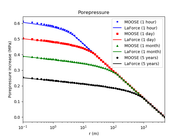
Figure 2: Comparison between the PorousFlow result and the analytic expression derived by LaForce et al. for the porepressure (Eq. (12) in LaForce et al. (2014b))
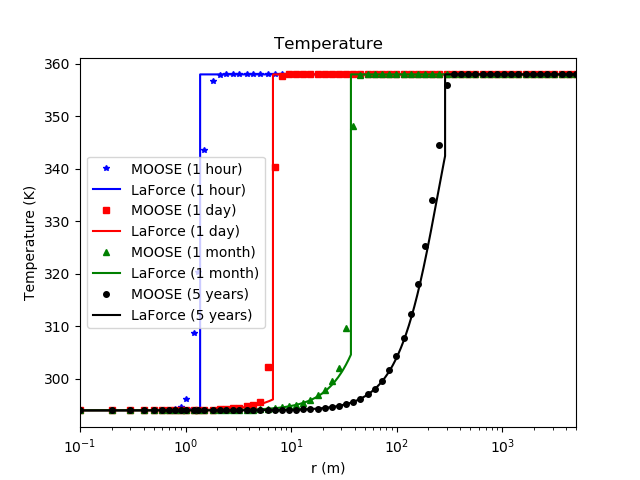
Figure 3: Comparison between the PorousFlow result and the analytic expression derived by LaForce et al. for the temperature (Eq. (20) in LaForce et al. (2014a))
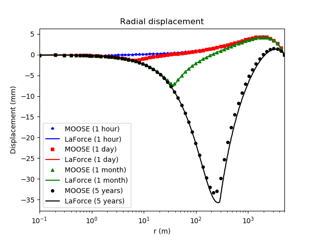
Figure 4: Comparison between the PorousFlow result and the analytic expression derived by LaForce et al. for the radial displacement (Eq. (33) in LaForce et al. (2014b))
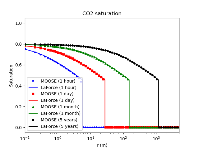
Figure 5: Comparison between the PorousFlow result and the analytic expression derived by LaForce et al. for the gas saturation (from Eq. (16) in LaForce et al. (2014a))
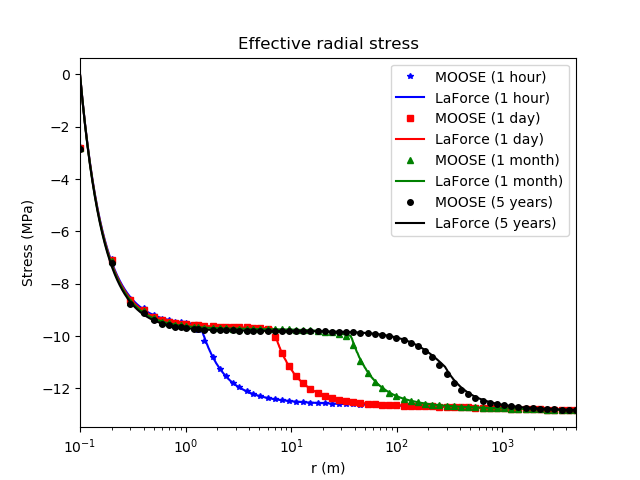
Figure 6: Comparison between the PorousFlow result and the analytic expression derived by LaForce et al. for the effective radial stress (Eq. (A3) in LaForce et al. (2014b)). The small discrepancy at the borehole wall is due to the finite resolution of the MOOSE model, where stresses are evaluated at finite-element centroids instead of at nodes.
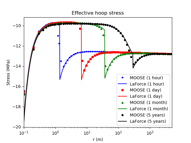
Figure 7: Comparison between the PorousFlow result and the analytic expression derived by LaForce et al. for the effective hoop stress (Eq. (A3) in LaForce et al. (2014b)). The small discrepancy at the borehole wall is due to the finite resolution of the MOOSE model, where stresses are evaluated at finite-element centroids instead of at nodes.
Acknowledgement
The authors wish to acknowledge financial assistance provided through Australian National Low Emissions Coal Research and Development ANLEC R&D. ANLEC R&D is supported by Australian Coal Association Low Emissions Technology Limited and the Australian Government through the Clean Energy Initiative.
A chemically-reactive, elastic reservoir
Another page describes how the model of this page may be extended to include geochemical reactions in the reservoir.
References
- T. LaForce, J. Ennis-King, and L. Paterson.
Semi-analytical solutions for nonisothermal fluid injection including heat loss from the reservoir: Part 1. Saturation and temperature.
Advances in Water Resources, 73:227–234, 2014a.[BibTeX]
@article{laforce2014a, author = "LaForce, T. and Ennis-King, J. and Paterson, L.", title = "{Semi-analytical solutions for nonisothermal fluid injection including heat loss from the reservoir: Part 1. Saturation and temperature}", journal = "Advances in Water Resources", volume = "73", pages = "227--234", year = "2014a" } - T. LaForce, A. Mijic, J. Ennis-King, and L. Paterson.
Semi-analytical solutions for nonisothermal fluid injection including heat loss from the reservoir: Part 2. Pressure and stress.
Advances in Water Resources, 73:242–253, 2014b.[BibTeX]
@article{laforce2014b,
    author = "LaForce, T. and Mijic, A. and Ennis-King, J. and Paterson, L.",
    title = "{Semi-analytical solutions for nonisothermal fluid injection including heat loss from the reservoir: Part 2. Pressure and stress}",
    journal = "Advances in Water Resources",
    volume = "73",
    pages = "242--253",
    year = "2014b"
}
(modules/porous_flow/examples/thm_example/2D.i)
# Two phase, temperature-dependent, with mechanics, radial with fine mesh, constant injection of cold co2 into a overburden-reservoir-underburden containing mostly water
# species=0 is water
# species=1 is co2
# phase=0 is liquid, and since massfrac_ph0_sp0 = 1, this is all water
# phase=1 is gas, and since massfrac_ph1_sp0 = 0, this is all co2
#
# The mesh used below has very high resolution, so the simulation takes a long time to complete.
# Some suggested meshes of different resolution:
# nx=50, bias_x=1.2
# nx=100, bias_x=1.1
# nx=200, bias_x=1.05
# nx=400, bias_x=1.02
# nx=1000, bias_x=1.01
# nx=2000, bias_x=1.003
[Mesh]
  type = GeneratedMesh
  dim = 2
  nx = 2000
  bias_x = 1.003
  xmin = 0.1
  xmax = 5000
  ny = 1
  ymin = 0
  ymax = 11
[]

[Problem]
  coord_type = RZ
[]

[GlobalParams]
  displacements = 'disp_r disp_z'
  PorousFlowDictator = dictator
  gravity = '0 0 0'
  biot_coefficient = 1.0
[]

[Variables]
  [pwater]
    initial_condition = 18.3e6
  []
  [sgas]
    initial_condition = 0.0
  []
  [temp]
    initial_condition = 358
  []
  [disp_r]
  []
[]

[AuxVariables]
  [rate]
  []
  [disp_z]
  []
  [massfrac_ph0_sp0]
    initial_condition = 1 # all H20 in phase=0
  []
  [massfrac_ph1_sp0]
    initial_condition = 0 # no H2O in phase=1
  []
  [pgas]
    family = MONOMIAL
    order = FIRST
  []
  [swater]
    family = MONOMIAL
    order = FIRST
  []
  [stress_rr]
    order = CONSTANT
    family = MONOMIAL
  []
  [stress_tt]
    order = CONSTANT
    family = MONOMIAL
  []
  [stress_zz]
    order = CONSTANT
    family = MONOMIAL
  []
[]

[Kernels]
  [mass_water_dot]
    type = PorousFlowMassTimeDerivative
    fluid_component = 0
    variable = pwater
  []
  [flux_water]
    type = PorousFlowAdvectiveFlux
    fluid_component = 0
    use_displaced_mesh = false
    variable = pwater
  []
  [mass_co2_dot]
    type = PorousFlowMassTimeDerivative
    fluid_component = 1
    variable = sgas
  []
  [flux_co2]
    type = PorousFlowAdvectiveFlux
    fluid_component = 1
    use_displaced_mesh = false
    variable = sgas
  []
  [energy_dot]
    type = PorousFlowEnergyTimeDerivative
    variable = temp
  []
  [advection]
    type = PorousFlowHeatAdvection
    use_displaced_mesh = false
    variable = temp
  []
  [conduction]
    type = PorousFlowExponentialDecay
    use_displaced_mesh = false
    variable = temp
    reference = 358
    rate = rate
  []
  [grad_stress_r]
    type = StressDivergenceRZTensors
    temperature = temp
    eigenstrain_names = thermal_contribution
    variable = disp_r
    use_displaced_mesh = false
    component = 0
  []
  [poro_r]
    type = PorousFlowEffectiveStressCoupling
    variable = disp_r
    use_displaced_mesh = false
    component = 0
  []
[]

[AuxKernels]
  [rate]
    type = FunctionAux
    variable = rate
    execute_on = timestep_begin
    function = decay_rate
  []
  [pgas]
    type = PorousFlowPropertyAux
    property = pressure
    phase = 1
    variable = pgas
  []
  [swater]
    type = PorousFlowPropertyAux
    property = saturation
    phase = 0
    variable = swater
  []
  [stress_rr]
    type = RankTwoAux
    rank_two_tensor = stress
    variable = stress_rr
    index_i = 0
    index_j = 0
  []
  [stress_tt]
    type = RankTwoAux
    rank_two_tensor = stress
    variable = stress_tt
    index_i = 2
    index_j = 2
  []
  [stress_zz]
    type = RankTwoAux
    rank_two_tensor = stress
    variable = stress_zz
    index_i = 1
    index_j = 1
  []
[]

[Functions]
  [decay_rate]
# Eqn(26) of the first paper of LaForce et al.
# Ka * (rho C)_a = 10056886.914
# h = 11
    type = ParsedFunction
    value = 'sqrt(10056886.914/t)/11.0'
  []
[]

[UserObjects]
  [dictator]
    type = PorousFlowDictator
    porous_flow_vars = 'temp pwater sgas disp_r'
    number_fluid_phases = 2
    number_fluid_components = 2
  []
  [pc]
    type = PorousFlowCapillaryPressureConst
    pc = 0
  []
[]

[Modules]
  [FluidProperties]
    [water]
      type = SimpleFluidProperties
      bulk_modulus = 2.27e14
      density0 = 970.0
      viscosity = 0.3394e-3
      cv = 4149.0
      cp = 4149.0
      porepressure_coefficient = 0.0
      thermal_expansion = 0
    []
    [co2]
      type = SimpleFluidProperties
      bulk_modulus = 2.27e14
      density0 = 516.48
      viscosity = 0.0393e-3
      cv = 2920.5
      cp = 2920.5
      porepressure_coefficient = 0.0
      thermal_expansion = 0
    []
  []
[]

[Materials]
  [temperature]
    type = PorousFlowTemperature
    temperature = temp
  []
  [ppss]
    type = PorousFlow2PhasePS
    phase0_porepressure = pwater
    phase1_saturation = sgas
    capillary_pressure = pc
  []
  [massfrac]
    type = PorousFlowMassFraction
    mass_fraction_vars = 'massfrac_ph0_sp0 massfrac_ph1_sp0'
  []
  [water]
    type = PorousFlowSingleComponentFluid
    fp = water
    phase = 0
  []
  [gas]
    type = PorousFlowSingleComponentFluid
    fp = co2
    phase = 1
  []
  [porosity_reservoir]
    type = PorousFlowPorosityConst
    porosity = 0.2
  []
  [permeability_reservoir]
    type = PorousFlowPermeabilityConst
    permeability = '2e-12 0 0  0 0 0  0 0 0'
  []
  [relperm_liquid]
    type = PorousFlowRelativePermeabilityCorey
    n = 4
    phase = 0
    s_res = 0.200
    sum_s_res = 0.405
  []
  [relperm_gas]
    type = PorousFlowRelativePermeabilityBC
    phase = 1
    s_res = 0.205
    sum_s_res = 0.405
    nw_phase = true
    lambda = 2
  []
  [thermal_conductivity_reservoir]
    type = PorousFlowThermalConductivityIdeal
    dry_thermal_conductivity = '0 0 0  0 1.320 0  0 0 0'
    wet_thermal_conductivity = '0 0 0  0 3.083 0  0 0 0'
  []
  [internal_energy_reservoir]
    type = PorousFlowMatrixInternalEnergy
    specific_heat_capacity = 1100
    density = 2350.0
  []
  [elasticity_tensor]
    type = ComputeIsotropicElasticityTensor
    shear_modulus = 6.0E9
    poissons_ratio = 0.2
  []
  [strain]
    type = ComputeAxisymmetricRZSmallStrain
    eigenstrain_names = 'thermal_contribution ini_stress'
  []
  [ini_strain]
    type = ComputeEigenstrainFromInitialStress
    initial_stress = '-12.8E6 0 0  0 -51.3E6 0  0 0 -12.8E6'
    eigenstrain_name = ini_stress
  []
  [thermal_contribution]
    type = ComputeThermalExpansionEigenstrain
    temperature = temp
    stress_free_temperature = 358
    thermal_expansion_coeff = 5E-6
    eigenstrain_name = thermal_contribution
  []
  [stress]
    type = ComputeLinearElasticStress
  []
  [eff_fluid_pressure]
    type = PorousFlowEffectiveFluidPressure
  []
  [vol_strain]
    type = PorousFlowVolumetricStrain
  []
[]

[BCs]
  [outer_pressure_fixed]
    type = DirichletBC
    boundary = right
    value = 18.3e6
    variable = pwater
  []
  [outer_saturation_fixed]
    type = DirichletBC
    boundary = right
    value = 0.0
    variable = sgas
  []
  [outer_temp_fixed]
    type = DirichletBC
    boundary = right
    value = 358
    variable = temp
  []
  [fixed_outer_r]
    type = DirichletBC
    variable = disp_r
    value = 0
    boundary = right
  []
  [co2_injection]
    type = PorousFlowSink
    boundary = left
    variable = sgas
    use_mobility = false
    use_relperm = false
    fluid_phase = 1
    flux_function = 'min(t/100.0,1)*(-2.294001475)' # 5.0E5 T/year = 15.855 kg/s, over area of 2Pi*0.1*11
  []
  [cold_co2]
    type = DirichletBC
    boundary = left
    variable = temp
    value = 294
  []
  [cavity_pressure_x]
    type = Pressure
    boundary = left
    variable = disp_r
    component = 0
    postprocessor = p_bh # note, this lags
    use_displaced_mesh = false
  []
[]

[Postprocessors]
  [p_bh]
    type = PointValue
    variable = pwater
    point = '0.1 0 0'
    execute_on = timestep_begin
    use_displaced_mesh = false
  []
[]

[VectorPostprocessors]
  [ptsuss]
    type = LineValueSampler
    use_displaced_mesh = false
    start_point = '0.1 0 0'
    end_point = '5000 0 0'
    sort_by = x
    num_points = 50000
    outputs = csv
    variable = 'pwater temp sgas disp_r stress_rr stress_tt'
  []
[]

[Preconditioning]
  active = 'smp'
  [smp]
    type = SMP
    full = true
    #petsc_options = '-snes_converged_reason -ksp_diagonal_scale -ksp_diagonal_scale_fix -ksp_gmres_modifiedgramschmidt -snes_linesearch_monitor'
    petsc_options_iname = '-ksp_type -pc_type -sub_pc_type -sub_pc_factor_shift_type -pc_asm_overlap -snes_atol -snes_rtol -snes_max_it'
    petsc_options_value = 'gmres      asm      lu           NONZERO                   2               1E2       1E-5        500'
  []
  [mumps]
    type = SMP
    full = true
    petsc_options = '-snes_converged_reason -ksp_diagonal_scale -ksp_diagonal_scale_fix -ksp_gmres_modifiedgramschmidt -snes_linesearch_monitor'
    petsc_options_iname = '-ksp_type -pc_type -pc_factor_mat_solver_package -pc_factor_shift_type -snes_rtol -snes_atol -snes_max_it'
    petsc_options_value = 'gmres      lu       mumps                         NONZERO               1E-5       1E2       50'
  []
[]

[Executioner]
  type = Transient
  solve_type = NEWTON
  end_time = 1.5768e8
  #dtmax = 1e6
  [TimeStepper]
    type = IterationAdaptiveDT
    dt = 1
    growth_factor = 1.1
  []
[]

[Outputs]
  print_linear_residuals = false
  sync_times = '3600 86400 2.592E6 1.5768E8'
  perf_graph = true
  exodus = true
  [csv]
    type = CSV
    sync_only = true
  []
[]