Groundwater models
Authors: Andy Wilkins and Maëlle Grass
The PorousFlow module may be used to simulate groundwater systems. A typical example can be found in Herron et al. (2018). Large and complex models may be built that include the effect of rainfall patterns, spatially and temporally varying evaporation and transpiration, seasonal river flows, realistic topography and hydrogeology, as well as human factors such as mines, water bores, dams, etc.
It is also possible to include the vadose zone (unsaturated flow), to track the transport of tracers and pollutants through the system (multi-component flow), to utilize high-precision equations of state for the groundwater (density and viscosity as functions of porepressure and temperature), to include heat flows, to include the impact of rock deformation (solid mechanics), to include gas flows (multi-phase flows) and geochemical reactions. This page concentrates mostly on the construction of traditional groundwater models and only touches lightly on these more elaborate options, which are explained in the other PorousFlow examples, tutorials and tests.
Groundwater concepts
Because PorousFlow has been built as a general multi-component, multi-phase simulator, its models and physics are most conveniently and commonly expressed in terms of quantities that are alien to many experienced groundwater modellers, such as porepressure, permeability and porosity. This section provides translations between more conventional concepts — hydraulic head, hydraulic conductivity and storativity — and the quantities usually used in PorousFlow simulations. In the following sections, PorousFlow models are presented using the conventional groundwater quantities (hydraulic head, etc) as well as the "natural" quantities (porepressure, etc) but for the reasons mentioned below, users are encouraged to use the "natural" quantities in their models.
Hydraulic head and porepressure
Many experienced groundwater modellers will be used to expressing their models in terms of hydraulic head. For instance, if a borehole is drilled into an aquifer that has a hydraulic head of 5m, then the groundwater in the borehole will rise 5m above the water table. (This is assuming the hydraulic head is measured relative to the local water table, which is the common convention.) This is shown in Figure 1.
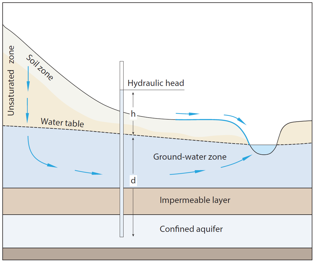
Figure 1: Hydraulic head, , of an aquifer is measured by recording the height above the water table (the datum in this case) of groundwater in a borehole.
Hydraulic head determines the direction of groundwater flow. For instance, if the hydraulic head of a sandstone aquifer is greater than a siltstone aquifer, groundwater will attempt to flow from the sandstone to the siltstone. Or, if the hydraulic gradient increases from south to north — that is, the hydraulic head is small in the southern regions and is large in the northern regions — then groundwater will tend to flow from north to south.
PorousFlow models are more naturally expressed in terms of porepressure, which is the pressure of the groundwater. This is related to hydraulic head through: (1) Here:
is porepressure, measured in Pa
is hydraulic head, with respect to a fixed datum such as the elevation above sea level of water table at a monitoring site, measured in m
is depth below the fixed datum, measured in m
is the water density (approximately 1000kg.m) and is the acceleration due to gravity (approximately 10m.s), so Pa.m. (Recall 1Pa = 1N.m = 1kg.m.s.)
Consider a confined aquifer with constant hydraulic head, . This means that the groundwater in a borehole will rise metres above the fixed datum (e.g. the local groundwater level), irrespective of where the borehole is drilled and how deep it is (assuming the well intersects this aquifer and not another one). Eq. (1) shows that porepressure increases with depth! This may be conceptually challenging for modellers used to hydraulic head. Remember, porepressure is the actual pressure of the groundwater. It increases with depth because of the weight of the groundwater sitting above it.
Porepressure is advantageous to use in PorousFlow because users will often like to enhance their models using the advanced inbuilt features of PorousFlow, such as
realistic equations of state for the water (or brine), in which density and viscosity are functions of porepressure
vadose-zone physics (unsaturated flow) which is is conventionally expressed in terms of porepressure
coupling with solid mechanics through the effective stress, which is expressed in terms of porepressure
Below, models are expressed in terms of hydraulic head and porepressure, but in order to facilitate easy extension of their models, users are encouraged to utilize porepressure.
Hydraulic conductivity and permeability
Imagine a pipe of cross-sectional area filled with porous material, as shown in Figure 2 Assume there is a constant hydraulic gradient between its ends: Darcy's law states that the flow rate of water, , is proportional to the hydraulic gradient: (2) In this equation:
is the flow rate of water through the pipe, measured in m.s
is the cross-sectional area of the pipe, measured in m
is the hydraulic conductivity of the porous material inside the pipe, measured in m.s
is the hydraulic gradient, and the negative sign indicates water flows from regions of high head to low head.
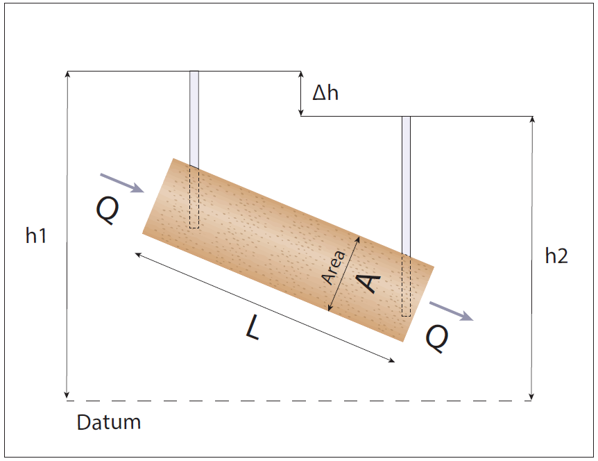
Figure 2: Darcy flow, , through a pipe of cross-sectional area due to a hydraulic gradient.
To provide extra context for the meaning of hydraulic conductivity, imagine a vertical column of saturated porous material that is open at both ends. This could be the rock above an underground mine, for instance. Gravity will cause the water to move downwards (and be replaced by air at the top end). The hydraulic head in this situation is , where is the elevation (and the porepressure is zero, or atmospheric pressure), so . The flow of water per unit area is therefore That is, under gravity-driven flow, the flow-rate of water controlled by , measured in m(water)/m(area)/s.
The physics of PorousFlow is more naturally presented in terms of permeability rather than hydraulic conductivity. Permeability is an intrinsic quantity of a porous material, in contrast to hydraulic conductivity, which only pertains to water. Permeability is therefore useful in multi-phase systems that may not even include water, and in situations where the fluids do not have constant density. Hence, permeability is usually used in the petroleum literature, geothermal scenarios (where the density of water is varying), unconventional-gas models, etc.
Writing Eq. (2) using the porepressure of Eq. (1) yields In these equations:
it is assumed that depth, , does not depend on . If the axis were oriented vertically then the equations would include instead of just .
is the permeability, measured in m.
is the water dynamic viscosity, measured in Pa.s.
The relationship between the permeability and hydraulic conductivity is therefore: (3) where is the density of water and is its dynamic viscosity.
Permeability is often measured in Darcys instead of its natural unit of m. The conversion is
Both permeability and hydraulic conductivity are tensors, so PorousFlow demands that users enter the full tensorial quantity, even though for most cases this is of the form
permeability = 'horizontal_x 0 0 0 horizontal_y 0 0 0 vertical'
Storativity and porosity
A porous material like rock is conceptualised as consisting of solid rock grains and void space. Groundwater flows through the void space. Both storativity and porosity parameterise the amount of groundwater present in a volume of porous material.
Porosity is defined as: Here
is the porosity, which is dimensionless
is the volume of connected void space, measured in m. (There may also be unconnected void spaces, which are ignored in this presentation since they are unimportant for fluid flow and only impact the solid-mechanical deformations.)
is the volume of the porous material (rock) sample, measured in m
is the volume of the solid grains (containing no void space), measured in m
Hence, if the porous material is fully saturated with water at atmospheric pressure, it contains a volume of of water at atmospheric pressure.
However, in the general situation, the volume of water that can be extracted from a volume of porous material is often not because of the following.
The porous material may not be fully saturated with water, meaning that the water volume is less than
Even if fully saturated, the water may be under high pressure, and since it is slightly compressible and the rock grains are slightly compressible, the water volume at atmospheric pressure may be greater than . Similarly, because of the compressibilities, can depend on porepressure, so the that is measured at atmospheric pressure in a lab may be different than the in-situ .
Due to unsaturated physics — namely capillarity and relative permeability — it may be impossible to extract all the water without resorting to extreme pressures, temperatures or chemical stimulants.
All these phenomena are handled automatically by PorousFlow, so porosity is usually employed in PorousFlow models. Porosity is also a natural quantity to use in multi-phase flow scenarios. In most groundwater models, porosity or its cousin, the BiotModulus, are simply specified as fixed quantities for each hydrologic unit. In more elaborate models, porosity is specified at atmospheric pressure and temperature, at zero strain, and in-situ amount of mineralisation, and a PorousFlowPorosity Material handles any changes due to changes in porepressure, temperature, deformation and dissolution/precipitation.
However, for the 3 reasons stated above, storativity, specific yield and specific storage are often used instead of porosity in groundwater models, reports and literature. These are defined as follows.
Storativity or storage coefficient
Here
is the storativity, which is sometimes called the storage coefficient, which is dimensionless
is the specific storage, measured in m
is the aquifer thickness, measured in m
is the specific yield, which is dimensionless
Specific storage
(4) The symbol has been used instead of equality to emphasise that various assumptions have been made concerning the interaction between water pressure and solid-mechanical stresses and strains. In this formula:
is the specific storage, measured in m
is the water density (approximately 1000kg.m) and is the acceleration due to gravity (approximately 10m.s), so Pa.m.
is the compressibility of the rock grains (the porous material without any void space), which is the reciprocal of its bulk modulus, measured in Pa. Typical values are Pa for clay, Pa for sandstone, Pa for shale, Pa for limestone and granite.
is the compressibility of water (approximately Pa), measured in Pa.
Specific yield
Specific yield, , is the volume of water that can be drained by gravity from a volume of porous material. It is therefore close to the porosity, . However, due to unsaturated physics, it is typically a little less than .
Groundwater equations for confined situations
If you dislike equations as much as many groundwater hydrogeologists feel free to read the following note and skip to the next section!
There are many different versions of the groundwater flow equations, and even more numerical implementations of them. Each produces slightly different solutions. The differences are tiny compared with the uncertainties in input parameters such as an aquifer's hydraulic conductivity.
Groundwater models often consider only fully-saturated scenarios such as confined aquifers, and do not consider the vadose zone. This section contains a number of versions of the physical equations governing the groundwater flow in such situations.
These equations are sometimes used to model unsaturated flow (as in unconfined aquifers) however, strictly speaking their physics does not accurately describe such flows. Using the equations below for both saturated and unsaturated zones means your model will be simple and will run rapidly. The porepressure will be positive in fully-saturated regions, and negative in unsaturated regions. If required, you will need to invent your own relationship between saturation and the negative porepressure. Alternately, you may use a PorousFlowUnsaturated Action instead of a PorousFlow BasicTHM to accurately simulate models with both saturated and unsaturated zones, at the cost of providing extra information (the capillary and relative permeability functions) and computational speed.
Presentation 1
Groundwater flow is often modelled by the equation (5) Here:
is time, measured in s
is the porosity, which is dimensionless. It may vary spatially, corresponding to different aquifers and aquitards, for instance.
is the water density, measured in kg.m
is a vector of spatial derivatives, , measured in m. The index is 1, 2 or 3, depending on the spatial direction. If the situation is 2D then the sums in Eq. (5) run over 1 and 2 only.
is the permeability tensor, , measured in m. Usually this is transversely isotropic:
is the viscosity of water, measured in Pa.s
is the porepressure
is the acceleration due to gravity, measured in kg.m.s. If the axis points upwards, this is (i.e., points in the direction of falling).
Presentation 2
Eq. (5) may be extended to the situation in which the porous-material (rock) grains are compressible and may suffer volumetric expansion or compaction due to changes in groundwater porepressure. In this case the equation reads (6) In this equation is the volumetric strain of the porous material.
Presentation 3
As described here, various standard assumptions allow the left-hand side of Eq. (6) to be re-written: (7) In this equation is the so-called Biot modulus, measured in Pa: (8) Here:
is the porosity
is the compressibility of water (approximately Pa), measured in Pa.
is the compressibility of the rock grains (the porous material without any void space), which is the reciprocal of its bulk modulus, measured in Pa.
is the Biot coefficient, which is dimensionless, and describes the impact of the groundwater on solid-mechanical stresses. is usually chosen within the range . If then the groundwater has maximum impact on the solid-mechanical stresses.
In groundwater scenarios, the Biot modulus may be considered time-independent and only dependent on the porous material via material-dependent and .
Presentation 4
Assuming the density of water has very little spatial variation, it may be divided out from Eq. (9) leaving a diffusion equation: (10)
Presentation 5
Notice the similarity of Eq. (4) and Eq. (8). To reasonable accuracy (11) Hence Eq. (9) may be written (12)
Presentation 6
Using the definition of hydraulic head, Eq. (1), and hydraulic conductivity, Eq. (3) in Eq. (12), and making further assumptions based on the almost-incompressibility of water yields the usual groundwater flow equation (13)
Simulating a pumping test
To illustrate the basic setup of a PorousFlow groundwater model, an aquifer pumping test. This example forms part of the PorousFlow QA test suite and is documented from that perspective here.
Place a constant volumetric sink of strength (m.m.s) acting along an infinite line in an isotropic 3D medium. The situation is therefore two dimensional. Assuming that groundwater head obeys Eq. (13), Theis provided the solution for the head (14) which is frequently used in the groundwater literature. "Ei" is the exponential integral function, with values for small (where is the Euler number ), and for large .
A sketch of the modelled situation is shown in Figure 3.
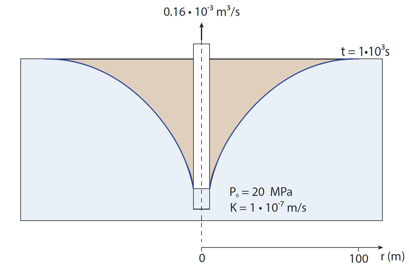
Figure 3: Sketch of a pumping test. A well extracts water at a constant rate from an aquifer with initial porepressure 20MPa, which causes drawdown, as shown by the blue curve.
The MOOSE input file may be broken down into a number of sections, as follows.
The mesh
The situation is two dimensional, but radially symmetric, so can be simulated using a one-dimensional mesh, with a single radial coordinate:
[Mesh]
  type = GeneratedMesh
  dim = 1
  nx = 20
  xmax = 100
  bias_x = 1.05
[]

[Problem]
  coord_type = RZ
[]
The PorousFlowDictator
All PorousFlow input files must include a PorousFlowDictator. This specifies the number of fluid phases (1 for groundwater models), number of fluid components (1 for groundwater models without tracers) and various other things that enable consistency checking throughout the input file. Virtually all PorousFlow objects require a PorousFlowDictator input parameter. Hence, to shorten input files, virtually all PorousFlow input files contain the PorousFlowDictator information in their GlobalParams block:
[GlobalParams]
  PorousFlowDictator = dictator
[]
This simply means you do not have to type PorousFlowDictator = dictator in all the other PorousFlow objects in your input files.
The physics
In order to replicate Eq. (14), the physics needs to be described by Eq. (13). This may be achieved by employing a PorousFlowBasicTHM Action:
[PorousFlowBasicTHM]
  dictator_name = dictator
  add_darcy_aux = false
  fp = simple_fluid
  gravity = '0 0 0'
  multiply_by_density = false
  porepressure = pp
[]
At this stage, it is probably a good idea for readers to skim-read the description of the PorousFlowBasicTHM Action, as it will be used extensively in this page.
The Action implements Eq. (9). The Action also implements coupling with solid mechanics and heat flow, which are not of interest in simple groundwater models. To ignore these couplings, simply do not specify the coupling_type input parameter, since it defaults to hydro. Note the flags:
  gravity = '0 0 0'
  multiply_by_density = false
which mean that Eq. (9) becomes (in 1D, without the and indices) This is of the same form as Eq. (13) if the relationships mentioned above are used (with Pa.m and Pa.s), namely:
Hence, the action is implementing the desired equation, assuming the parameters and are chosen appropriately.
Some additional remarks are:
The Action also implements Eq. (10) when the flag
multiply_by_density = false.The Action also implements Eq. (12) when the Biot Modulus (see below) is set to as in Eq. (11)
The Action does not have a "hydraulic head" input parameter. Instead, it assumes that modellers are using "porepressure", users must supply the name of the porepressure variable using the
porepressure = XXXXinput (hereXXXXis the name of the porepressure variable).In the above block
add_darcy_aux = falseis used simply because the QA test does not involve checking the Darcy-velocity directions. Usually you will want to omit this line and PorousFlow will automatically add Darcy-velocity information to your output.
Variables
In this input file, and most groundwater input files, there is just one Variable (unknown to solve for). It is called pp here, although it may be interpreted as hydraulic head using the scaling :
[Variables]
  [pp]
    initial_condition = 20E6
  []
[]
Equation of state for water
PorousFlow requires users to specify their "equation of state". These are functional relationships that provide density and viscosity (and thermal conductivity, enthalpy, etc) as functions of porepressure and temperature. In virtually all groundwater models a SimpleFluidProperties object is sufficient:
[Modules]
  [FluidProperties]
    [simple_fluid]
      type = SimpleFluidProperties
      viscosity = 0.001
    []
  []
[]
Here:
the
viscosityis specified exactly, to make the relationship clearer in this example.the name
simple_fluidis provided to the PorousFlowBasicTHM, above
Material properties
The permeability and Biot Modulus need to be specified. This is always done via a Materials block:
[Materials]
  [porosity]
    type = PorousFlowPorosityConst
    porosity = 0.05
  []
  [biot_mod]
    type = PorousFlowConstantBiotModulus
    fluid_bulk_modulus = 2E9
    biot_coefficient = 1.0
  []
  [permeability]
    type = PorousFlowPermeabilityConst
    permeability = '1E-14 0 0 0 1E-14 0 0 0 1E-14'
  []
[]
In this case, setting porosity = 0.05, fluid_bulk_modulus = 2E9 and biot_coefficient = 1.0 means that the BiotModulus and the specific storage are The permeability is isotropic:
The produced water flux
This is implemented by a PorousFlowSquarePulsePointSource:
[DiracKernels]
  [sink]
    type = PorousFlowSquarePulsePointSource
    point = '0 0 0'
    mass_flux = -0.16E-3 # recall this is a volumetric flux because multiply_by_density = false in the Action, so this corresponds to a mass_flux of 0.16 kg/s/m because density=1000
    variable = pp
  []
[]
In this 2D case with multiply_by_density = false, this means m of water is removed from every 1m of aquifer height every second. If multiply_by_density = true and the model was 2D then the mass_flux in a PorousFlowSquarePulsePointSource would be measured in kg.s.m, and if the model was 3D the units would be kg.s.
The entire input file
The remainder of the input file involves the usual MOOSE objects, such as an Executioner to define the end time and time-stepping, as well as a Preconditioning block, and some output objects. The entire input file reads:
# Theis problem: Flow to single sink using BasicTHM
# SinglePhase
# RZ mesh

[Mesh]
  type = GeneratedMesh
  dim = 1
  nx = 20
  xmax = 100
  bias_x = 1.05
[]

[Problem]
  coord_type = RZ
[]

[GlobalParams]
  PorousFlowDictator = dictator
[]

[Variables]
  [pp]
    initial_condition = 20E6
  []
[]

[PorousFlowBasicTHM]
  dictator_name = dictator
  add_darcy_aux = false
  fp = simple_fluid
  gravity = '0 0 0'
  multiply_by_density = false
  porepressure = pp
[]

[Modules]
  [FluidProperties]
    [simple_fluid]
      type = SimpleFluidProperties
      viscosity = 0.001
    []
  []
[]

[Materials]
  [porosity]
    type = PorousFlowPorosityConst
    porosity = 0.05
  []
  [biot_mod]
    type = PorousFlowConstantBiotModulus
    fluid_bulk_modulus = 2E9
    biot_coefficient = 1.0
  []
  [permeability]
    type = PorousFlowPermeabilityConst
    permeability = '1E-14 0 0 0 1E-14 0 0 0 1E-14'
  []
[]

[DiracKernels]
  [sink]
    type = PorousFlowSquarePulsePointSource
    point = '0 0 0'
    mass_flux = -0.16E-3 # recall this is a volumetric flux because multiply_by_density = false in the Action, so this corresponds to a mass_flux of 0.16 kg/s/m because density=1000
    variable = pp
  []
[]

[VectorPostprocessors]
  [pp]
    type = LineValueSampler
    num_points = 25
    start_point = '0 0 0'
    end_point = '100 0 0'
    sort_by = x
    variable = pp
  []
[]

[Preconditioning]
  [smp]
    type = SMP
    full = true
  []
[]

[Executioner]
  type = Transient
  solve_type = Newton
  dt = 200
  end_time = 1E3
  nl_abs_tol = 1e-10
[]

[Outputs]
  perf_graph = true
  [csv]
    type = CSV
    execute_on = final
  []
[]
The results
MOOSE agrees with the Theis solution:
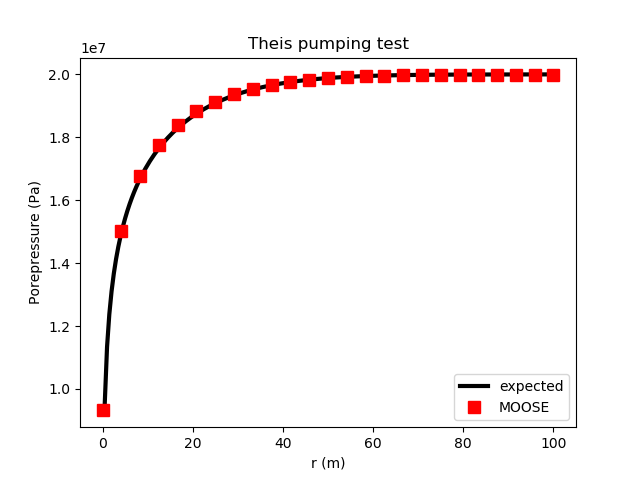
Figure 4: Results of the aquifer pumping test in comparison with the Theis solution.
Abstracting from a groundwater system
In this section, a model of the groundwater system shown in Figure 5 is studied.
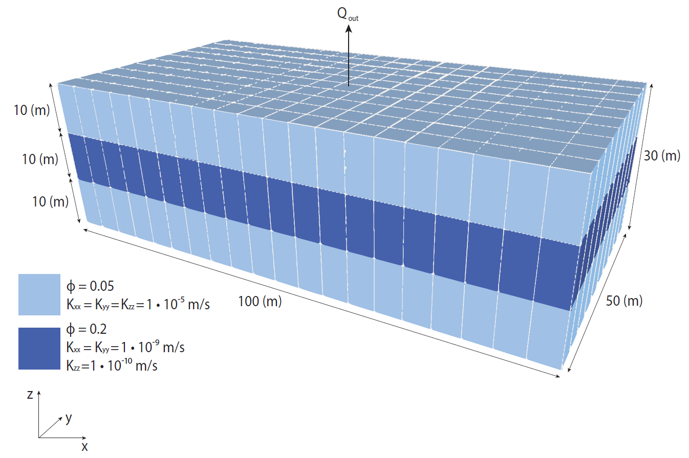
Figure 5: The mesh and properties used in the abstraction example.
The system consists of:
An upper aquifer of thickness 10m with porosity, , and isotropic permeability m. With Biot coefficient and water bulk compliance Pa, Eq. (8) implies the Biot modulus is GPa, and Eq. (11) implies the specific storage is m. This number is also produced by Eq. (4) if (Eq. (4) does not contain the Biot coefficient: it approximates ). Using Eq. (3), the hydraulic conductivity is m.day.
An aquitard of thickness 10m with porosity , horizontal permeability m and vertical permeability m. Using the same manipulations as in the preceding paragraph, this yields Biot modulus GPa, specific storage m, horizontal permeability mm.day and mm.day.
A lower aquifer of thickness 10m with the same physical parameters as the upper aquifer.
This system is assumed to exist in isolation from any other aquifers and aquitards. The roof of the upper aquifer is 70m below the water table.
A borehole abstracts water from either the lower aquifer or the aquitard (due to a mistake in the drilling or wellbore completion) and a model is built to investigate the drawdown in the upper aquifer due to these two scenarios.
The finite-element mesh
Creating the mesh is the most difficult aspect of numerical modelling in almost all models, be they groundwater models, structural-mechanical models, models of fluid turbulence, electromagnetic models, etc. For instance, the groundwater model in Herron et al. (2018) took about 3 months to construct since it contained over 100 underground mine workings, many aquifers and aquitards, streams and rivers and alluvium, zones of different evapotranspiration, the ocean, thousands of boreholes, etc. For groundwater modelling, only conceptualisation and parameterisation are more difficult, but these also impact the mesh, for example, there is no need to distinguish between different aquifers if their hydraulic conductivities are the same, up to measurement accuracy.
In this case, the mesh is very simple and may be created using MOOSE's inbuilt commands with the result shown in Figure 5:
[Mesh]
  [basic_mesh]
    type = GeneratedMeshGenerator
    dim = 3
    xmin = -50
    xmax = 50
    nx = 20
    ymin = -25
    ymax = 25
    ny = 10
    zmin = -100
    zmax = -70
    nz = 3
  []
  [lower_aquifer]
    type = SubdomainBoundingBoxGenerator
    input = basic_mesh
    block_id = 1
    block_name = lower_aquifer
    bottom_left = '-1000 -500 -100'
    top_right = '1000 500 -90'
  []
  [aquitard]
    type = SubdomainBoundingBoxGenerator
    input = lower_aquifer
    block_id = 2
    block_name = aquitard
    bottom_left = '-1000 -500 -90'
    top_right = '1000 500 -80'
  []
  [upper_aquifer]
    type = SubdomainBoundingBoxGenerator
    input = aquitard
    block_id = 3
    block_name = upper_aquifer
    bottom_left = '-1000 -500 -80'
    top_right = '1000 500 -70'
  []
[]
Equation of state for water
PorousFlow requires users to specify their "equation of state". These are functional relationships that provide density and viscosity (and thermal conductivity, enthalpy, etc) as functions of porepressure and temperature. In virtually all groundwater models a SimpleFluidProperties object is sufficient. In this case, the fluid bulk modulus is chosen very large and the thermal expansion coefficient chosen to be zero so that the groundwater density is very close to 1000kg.m so that Pa.m.
[Modules]
  [FluidProperties]
    [simple_fluid]
      type = SimpleFluidProperties
      # the following mean that density = 1000 * exp(P / 1E15) ~ 1000
      thermal_expansion = 0
      bulk_modulus = 1E15
    []
  []
[]
PorousFlowDictator specification
Most objects in PorousFlow models require the PorousFlowDictator to be specified, so this is most efficiently accomplished through the GlobalParams block:
[GlobalParams]
  PorousFlowDictator = dictator
[]
Variables
The only MOOSE variable (unknown) in this situation is the porepressure.
[Variables]
  [pp]
  []
[]
The physics
It is assumed that groundwater obeys Eq. (10). This physics is implemented in PorousFlow by the PorousFlowBasicTHM Action with multiply_by_density = false:
[PorousFlowBasicTHM]
  fp = simple_fluid
  gravity = '0 0 -10'
  porepressure = pp
  multiply_by_density = false
[]
The physics is of the same form as Eq. (13) if the relationships mentioned above are used (with Pa.m and Pa.s), namely:
As mentioned in the section above, the Action does not have a "hydraulic head" input parameter. Instead, it assumes that modellers are using "porepressure", users must supply the name of the porepressure variable using the porepressure = XXXX input (here XXXX is the name of the porepressure variable).
In-situ conditions: hydraulic gradient
Assume that:
That the porepressure is related to hydraulic head via Eq. (1) with
The average hydraulic head in the upper aquifer is 10m and there is a hydraulic gradient of from east to west in the upper aquifer
The hydraulic head in the lower aquifer is 20m. This means the model is not at hydrostatic equilibrium which could be due to recharge into the lower aquifer from a hilly region outside the model
The hydraulic head in the aquitard is a linear combination of these two
The following functions then describe the in-situ conditions:
  [upper_aquifer_head]
    type = ParsedFunction
    value = '10 + x / 200'
  []
  [lower_aquifer_head]
    type = ParsedFunction
    value = '20'
  []
  [insitu_head]
    type = ParsedFunction
    vals = 'lower_aquifer_head upper_aquifer_head'
    vars = 'low up'
    value = 'if(z <= -90, low, if(z >= -80, up, (up * (z + 90) - low * (z + 80)) / (10.0)))'
  []
  [insitu_pp]
    type = ParsedFunction
    vals = 'insitu_head'
    vars = 'h'
    value = '(h - z) * 1E4'
  []
Initial and boundary conditions
Assume that the initial conditions are as specified by the insitu_pp Function describe above. Assume also that porepressure is fixed on the model's boundaries. This corresponds to a ready source of water that flows into the model from regions outside the model. The relevant input-file blocks are:
[ICs]
  [pp]
    type = FunctionIC
    variable = pp
    function = insitu_pp
  []
[]
[BCs]
  [pp]
    type = FunctionDirichletBC
    variable = pp
    function = insitu_pp
    boundary = 'left right top bottom front back'
  []
[]
Prescribing material properties: porosity and permeability
The material properties are prescribed using the following block
[Materials]
  [porosity_aquifers]
    type = PorousFlowPorosityConst
    porosity = 0.05
    block = 'upper_aquifer lower_aquifer'
  []
  [porosity_aquitard]
    type = PorousFlowPorosityConst
    porosity = 0.2
    block = aquitard
  []
  [biot_mod]
    type = PorousFlowConstantBiotModulus
    fluid_bulk_modulus = 2E9
    biot_coefficient = 1.0
  []
  [permeability_aquifers]
    type = PorousFlowPermeabilityConst
    permeability = '1E-12 0 0 0 1E-12 0 0 0 1E-12'
    block = 'upper_aquifer lower_aquifer'
  []
  [permeability_aquitard]
    type = PorousFlowPermeabilityConst
    permeability = '1E-16 0 0 0 1E-16 0 0 0 1E-17'
    block = aquitard
  []
[]
Note the aquitard has anisotropic permeability: m while m.
The abstraction well
An abstraction well may be modelled using a PorousFlow sink. The reader is encouraged to study the documentation on the PorousFlow sinks page in order to understand the following block, since boreholes are frequently used for injection or production in groundwater models. A PorousFlowPolyLineSink is used in this example:
[DiracKernels]
  [sink]
    type = PorousFlowPolyLineSink
    SumQuantityUO = volume_extracted
    point_file = ex01.bh_lower
    line_length = 10
    variable = pp
    # following produces a flux of 0 m^3(water)/m(borehole length)/s if porepressure = 0, and a flux of 1 m^3/m/s if porepressure = 1E9
    p_or_t_vals = '0 1E9'
    fluxes = '0 1'
  []
[]
1 0 0 -95
The ex01.bh_lower file contains just one line, and the sink sets line_length = 10 and line_direction = '0 0 1' (by default) so this corresponds to a vertical borehole of length 10m. The lines
    p_or_t_vals = '0 1E9'
    fluxes = '0 1'
mean that the borehole will extract a flux of 0m(water)/m(borehole)/s if the porepressure is zero or lower, and a flux of 1m(water)/m/s if the porepressure is 1GPa or higher. In between these two porepressures, the flux varies linearly. Hence, this will cause porepressure to reduce to close to zero before an equilibrium is found between the borehole extraction rate and the groundwater flux through the rock. If multiply_by_density = true was used in the PorousFlowBasicTHM, then the units of fluxes would be kg(water)/m(borehole)/s.
If a fixed flux was required instead, then fluxes = '1 1' could be used, or another of the PorousFlow sinks could be employed.
The appropriate PorousFlow sink must be used for your model, because they represent significantly different physics, so produce significantly different results. This example uses a PorousFlowPolyLineSink for a borehole, while virtually all real-life models would use a PorousFlowPeacemanBorehole instead. A rule of thumb is to use a PorousFlowPeacemanBorehole for boreholes, and a PorousFlowPolyLineSink for rivers. This is discussed further towards the bottom of this page.
It is common to refine the mesh around boreholes:
a refinement in the plan mesh allows the extent of drawdown cones to be more accurately predicted;
a refinement in the vertical mesh so that the screened section is captured by at least one finite element is recommended as it allows drawdown on vertical sections to be accurately simulated.
Such refinements are not mandatory. They are not performed in this example because only MOOSE's simple inbuilt meshing functionality is used. (Using the PorousFlowPolyLineSink just so happens to be fine in this model because the single Dirac point coincides with a node in the plane.)
Recording the drawdown
AuxVariables and a VectorPostprocessor are used to record the head change throughout the model:
[AuxVariables]
  [insitu_head]
  []
  [head_change]
  []
[]
[AuxKernels]
  [insitu_head]
    type = FunctionAux
    variable = insitu_head
    function = insitu_head
  []
  [head_change]
    type = ParsedAux
    args = 'pp insitu_head'
    use_xyzt = true
    function = 'pp / 1E4 + z - insitu_head'
    variable = head_change
  []
[]
[VectorPostprocessors]
  [drawdown]
    type = LineValueSampler
    variable = head_change
    start_point = '-50 0 -75'
    end_point = '50 0 -75'
    num_points = 101
    sort_by = x
  []
[]
The entire input file
For reference, the entire input file is:
# Groundwater extraction example.
# System consists of two confined aquifers separated by an aquitard
# There is a hydraulic gradient in the upper aquifer
# A well extracts water from the lower aquifer, and the impact on the upper aquifer is observed
# In the center of the model, the roof of the upper aquifer sits 70m below the local water table

[Mesh]
  [basic_mesh]
    type = GeneratedMeshGenerator
    dim = 3
    xmin = -50
    xmax = 50
    nx = 20
    ymin = -25
    ymax = 25
    ny = 10
    zmin = -100
    zmax = -70
    nz = 3
  []
  [lower_aquifer]
    type = SubdomainBoundingBoxGenerator
    input = basic_mesh
    block_id = 1
    block_name = lower_aquifer
    bottom_left = '-1000 -500 -100'
    top_right = '1000 500 -90'
  []
  [aquitard]
    type = SubdomainBoundingBoxGenerator
    input = lower_aquifer
    block_id = 2
    block_name = aquitard
    bottom_left = '-1000 -500 -90'
    top_right = '1000 500 -80'
  []
  [upper_aquifer]
    type = SubdomainBoundingBoxGenerator
    input = aquitard
    block_id = 3
    block_name = upper_aquifer
    bottom_left = '-1000 -500 -80'
    top_right = '1000 500 -70'
  []
[]

[GlobalParams]
  PorousFlowDictator = dictator
[]

[Variables]
  [pp]
  []
[]

[ICs]
  [pp]
    type = FunctionIC
    variable = pp
    function = insitu_pp
  []
[]

[BCs]
  [pp]
    type = FunctionDirichletBC
    variable = pp
    function = insitu_pp
    boundary = 'left right top bottom front back'
  []
[]

[Functions]
  [upper_aquifer_head]
    type = ParsedFunction
    value = '10 + x / 200'
  []
  [lower_aquifer_head]
    type = ParsedFunction
    value = '20'
  []
  [insitu_head]
    type = ParsedFunction
    vals = 'lower_aquifer_head upper_aquifer_head'
    vars = 'low up'
    value = 'if(z <= -90, low, if(z >= -80, up, (up * (z + 90) - low * (z + 80)) / (10.0)))'
  []
  [insitu_pp]
    type = ParsedFunction
    vals = 'insitu_head'
    vars = 'h'
    value = '(h - z) * 1E4'
  []
  [l_rate]
    type = ParsedFunction
    vals = 'm3_produced dt'
    vars = 'm3_produced dt'
    value = '1000 * m3_produced / dt'
  []
[]

[AuxVariables]
  [insitu_head]
  []
  [head_change]
  []
[]

[AuxKernels]
  [insitu_head]
    type = FunctionAux
    variable = insitu_head
    function = insitu_head
  []
  [head_change]
    type = ParsedAux
    args = 'pp insitu_head'
    use_xyzt = true
    function = 'pp / 1E4 + z - insitu_head'
    variable = head_change
  []
[]

[Postprocessors]
  [m3_produced]
    type = PorousFlowPlotQuantity
    uo = volume_extracted
    outputs = 'none'
  []
  [dt]
    type = TimestepSize
    outputs = 'none'
  []
  [l_per_s]
    type = FunctionValuePostprocessor
    function = l_rate
  []
[]

[VectorPostprocessors]
  [drawdown]
    type = LineValueSampler
    variable = head_change
    start_point = '-50 0 -75'
    end_point = '50 0 -75'
    num_points = 101
    sort_by = x
  []
[]

[PorousFlowBasicTHM]
  fp = simple_fluid
  gravity = '0 0 -10'
  porepressure = pp
  multiply_by_density = false
[]

[Modules]
  [FluidProperties]
    [simple_fluid]
      type = SimpleFluidProperties
      # the following mean that density = 1000 * exp(P / 1E15) ~ 1000
      thermal_expansion = 0
      bulk_modulus = 1E15
    []
  []
[]

[Materials]
  [porosity_aquifers]
    type = PorousFlowPorosityConst
    porosity = 0.05
    block = 'upper_aquifer lower_aquifer'
  []
  [porosity_aquitard]
    type = PorousFlowPorosityConst
    porosity = 0.2
    block = aquitard
  []
  [biot_mod]
    type = PorousFlowConstantBiotModulus
    fluid_bulk_modulus = 2E9
    biot_coefficient = 1.0
  []
  [permeability_aquifers]
    type = PorousFlowPermeabilityConst
    permeability = '1E-12 0 0 0 1E-12 0 0 0 1E-12'
    block = 'upper_aquifer lower_aquifer'
  []
  [permeability_aquitard]
    type = PorousFlowPermeabilityConst
    permeability = '1E-16 0 0 0 1E-16 0 0 0 1E-17'
    block = aquitard
  []
[]

[DiracKernels]
  [sink]
    type = PorousFlowPolyLineSink
    SumQuantityUO = volume_extracted
    point_file = ex01.bh_lower
    line_length = 10
    variable = pp
    # following produces a flux of 0 m^3(water)/m(borehole length)/s if porepressure = 0, and a flux of 1 m^3/m/s if porepressure = 1E9
    p_or_t_vals = '0 1E9'
    fluxes = '0 1'
  []
[]

[UserObjects]
  [volume_extracted]
    type = PorousFlowSumQuantity
  []
[]

[Preconditioning]
  [smp]
    type = SMP
    full = true
  []
[]

[Executioner]
  type = Transient
  solve_type = Newton
  [TimeStepper]
    type = SolutionTimeAdaptiveDT
    dt = 1.1E5
  []
  end_time = 3.456E5 # 4 days
  nl_abs_tol = 1E-13
[]

[Outputs]
  [csv]
    type = CSV
    file_base = ex01_lower_extraction
    execute_on = final
  []
[]
Results
Water is abstracted from the lower aquifer when point_file = ex01.bh_lower in the PorousFlowPolyLineSink. This production rate is approximately l.s, and the upper aquifer experiences very little drawdown. Water is abstracted from the aquitard when point_file = ex01.bh_aquitard in the PorousFlowPolyLineSink, which results in production rate of about l.s and significant drawdown in the upper aquifer. The drawdown cone reaches steady state after about 4 days, and is shown in Figure 6.
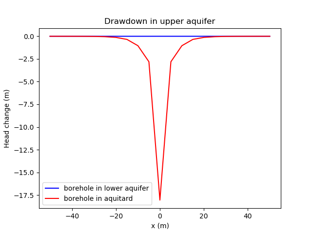
Figure 6: Drawdown in the upper aquifer when water is abstracted from the lower aquifer (blue line) or the aquitard (red line).
The results are mesh-dependent, as expected. A finer mesh produces more drawdown near to the well since it is more able to resolve spatial structure there.
The severe abstraction from the aquitard causes negative hydraulic head in the upper aquifer. This does not mean the porepressure is negative in this case. However, it is easy to build a model in which the porepressure becomes negative. This corresponds physically to desaturation, and to properly model such situations a PorousFlowUnsaturated Action should be used instead of a PorousFlowBasicTHM Action. In many cases, the extra computational cost of modelling unsaturated physics, and the difficulty of appropriately parameterising the model, mean that groundwater modellers choose to ignore partially-saturated physics and simply employ the equivalent of PorousFlowBasicTHM regardless of unsaturated zones. In PorousFlow it is relatively straightforward to swap between PorousFlowBasicTHM and PorousFlowUnsaturated to investigate the impact of including partially-saturated physics.
Baseflow, ET, recharge, unsaturated flow: impact of groundwater abstraction on baseflow to a river
In this example, the impact of groundwater abstraction on baseflow to a river is modelled. The hydrostratigraphy is shown in Figure 7. It consists of:
an upper, unconfined aquitard with topography of varying elevation representing a hill and valley
an aquitard that outcrops in the valley region
a lower aquifer that also outcrops in the valley region
The lower confined aquifer may be recharged by a perennial river that is assumed to exist at the valley's base. Or, it may provide baseflow to the river. Whether leakage or baseflow occurs depends on the groundwater porepressure: the position of the water table with respect to the river stage height.
A horizontal abstraction borehole is drilled into the lower aquifer below the river. The question to answer is: how does the groundwater abstraction influence the groundwater-river interaction? (Such horizontal boreholes are used in gas exploitation, but the main reason it is used here is to illustrate boreholes don't need to be vertical.)
To answer this question, the parameters defining the system will be described in the context of the PorousFlow input file, then the steady-state virgin system will be solved, then the borehole introduced and the impact assessed.
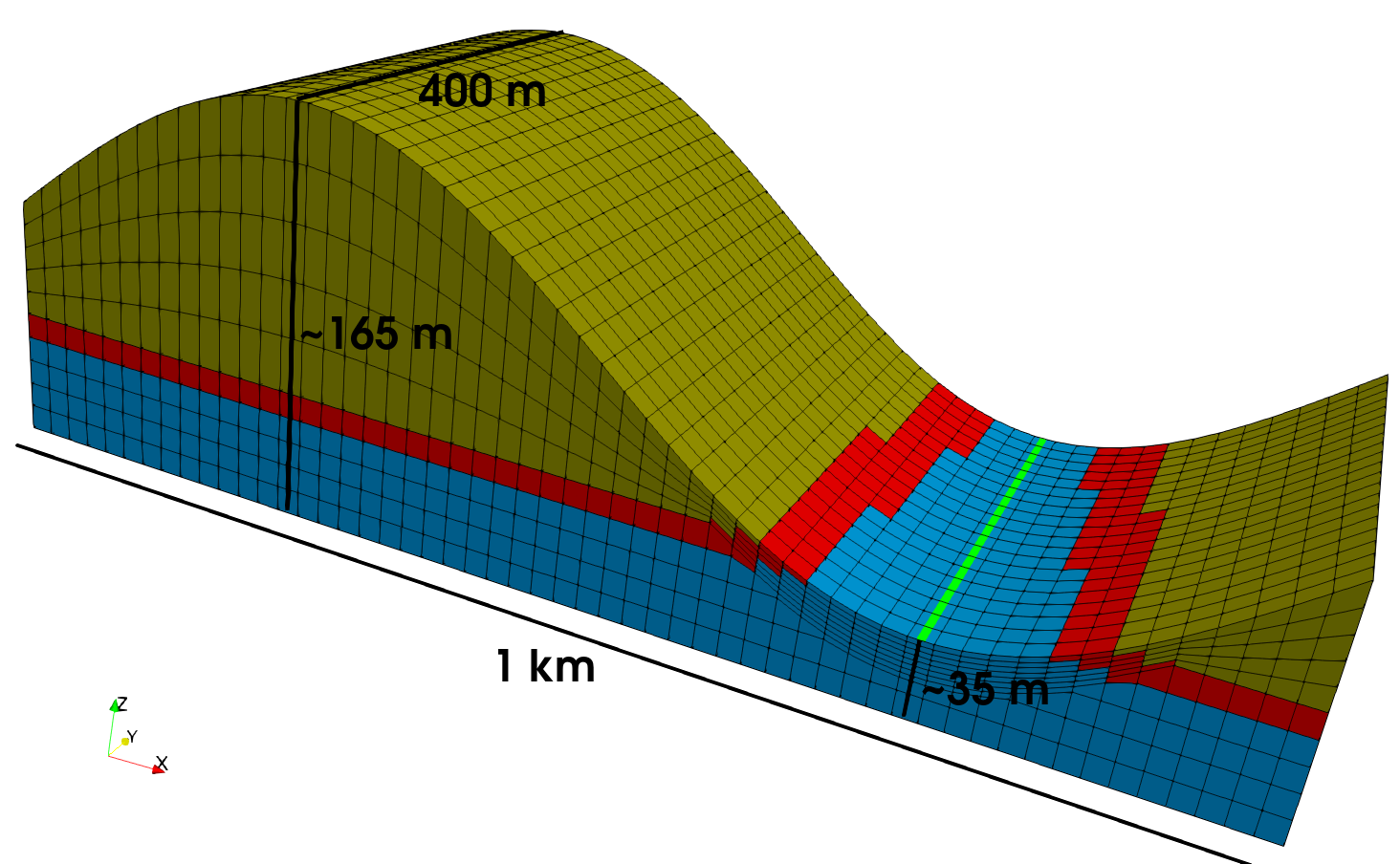
Figure 7: The hydrostratigraphy and the mesh used to explore the impact of groundwater abstraction on baseflow to the river. The unconfined aquifer is shown in brown-yellow, the aquitard in red and the confined aquifer in blue. The river is shown as a bright green line. Vertical exaggeration equals 2 in this figure. The mesh was created by a closed-source script built by CSIRO for these types of problems.
The mesh
The mesh in this case was created by an external program that defined the hydrogeology and the mesh, but not the boundaries that are required for this model. Hence, MOOSE's in-built MeshModifiers are used to identify the appropriate boundaries:
[Mesh]
  [basic_mesh]
    # mesh create by external program: lies within -500<=x<=500 and -200<=y<=200, with varying z
    type = FileMeshGenerator
    file = ex02_mesh.e
  []
  [name_blocks]
    type = RenameBlockGenerator
    input = basic_mesh
    old_block = '2 3 4'
    new_block = 'bot_aquifer aquitard top_aquifer'
  []
  [zmax]
    type = SideSetsFromNormalsGenerator
    input = name_blocks
    new_boundary = zmax
    normals = '0 0 1'
  []
  [xmin_bot_aquifer]
    type = ParsedGenerateSideset
    input = zmax
    included_subdomain_ids = 2
    normal = '-1 0 0'
    combinatorial_geometry = 'x <= -500.0'
    new_sideset_name = xmin_bot_aquifer
  []
[]
The physics
In this case, unsaturated flow and saturated flow are used, in order to use appropriate physics for the unconfined aquifer. Hence, instead of a PorousFlowBasicTHM Action, a PorousFlowUnsaturated action is used instead:
[PorousFlowUnsaturated]
  fp = simple_fluid
  porepressure = pp
[]
Readers are encouraged to read the documentation for the PorousFlowUnsaturated action if they need to model unsaturated flow. Usually, the above block would contain information concerning the relative permeability and the capillary pressure functions, sourced from site experiments, but in this case just the default values are used.
Note the important facet of PorousFlowUnsaturated: it does not have a multiply_by_density flag. Hence, all quantities are measured in mass, not volume. For instance, the recharge quantities are measured in kg.s, not m.s.
Porosity and permeability
The porosity is assumed to be 0.05 everywhere, while the permeabilities are assumed to be:
aquifers: m in the horizontal direction, m in the vertical direction
aquitard: m in the horizontal direction, m in the vertical direction
These properties are specified via:
[Materials]
  [porosity_everywhere]
    type = PorousFlowPorosityConst
    porosity = 0.05
  []
  [permeability_aquifers]
    type = PorousFlowPermeabilityConst
    block = 'top_aquifer bot_aquifer'
    permeability = '1E-12 0 0 0 1E-12 0 0 0 1E-13'
  []
  [permeability_aquitard]
    type = PorousFlowPermeabilityConst
    block = aquitard
    permeability = '1E-16 0 0 0 1E-16 0 0 0 1E-17'
  []
[]
Initial conditions
It is likely that the steady-state solution will be approximately hydrostatic. Therefore, to help PorousFlow converge, the model is initialized with the hydrostatic condition. This is non-trivial here because, for fixed elevation (), the depth varies spatially (with and ). The initial mesh, however, has depth information inserted into it, as the variable cosflow_depth. Hence, it may be extracted using a SolutionUserObject:
  [initial_mesh]
    type = SolutionUserObject
    execute_on = INITIAL
    mesh = ex02_mesh.e
    timestep = LATEST
    system_variables = cosflow_depth
  []
and then used in a Function:
  [initial_pp]
    type = SolutionFunction
    scale_factor = 1E4
    from_variable = cosflow_depth
    solution = initial_mesh
  []
before finally being used in an initial condition:
[ICs]
  [pp]
    type = FunctionIC
    variable = pp
    function = initial_pp
  []
[]
This kind of manipulation — using a SolutionUserObject and a SolutionFunction — is rather common in groundwater modelling.
Boundary conditions
The boundary conditions are the most complicated aspect of this input file.
Rainfall recharge
It is assumed that rainfall recharges the groundwater system at the topography with a constant rate of 0.1mm.day, uniformly over the entire topography. This quantity needs to be converted to a mass flux: Hence the BC:
  [rainfall_recharge]
    type = PorousFlowSink
    boundary = zmax
    variable = pp
    flux_function = -1E-6  # recharge of 0.1mm/day = 1E-4m3/m2/day = 0.1kg/m2/day ~ 1E-6kg/m2/s
  []
In most groundwater models, rainfall recharge would vary spatially and temporally, since different surficial expressions and vegetation cover and seasonal patterns impact rainfall recharge. This is easily incorporated through the flux_function or other parameters to the PorousFlowSink.
Evapotranspiration (ET)
A PorousFlowHalfCubicSink is used to model ET:
  [evapotranspiration]
    type = PorousFlowHalfCubicSink
    boundary = zmax
    variable = pp
    center = 0.0
    cutoff = -5E4 # roots of depth 5m.  5m of water = 5E4 Pa
    use_mobility = true
    fluid_phase = 0
    # Assume pan evaporation of 4mm/day = 4E-3m3/m2/day = 4kg/m2/day ~ 4E-5kg/m2/s
    # Assume that if permeability was 1E-10m^2 and water table at topography then ET acts as pan strength
    # Because use_mobility = true, then 4E-5 = maximum_flux = max * perm * density / visc = max * 1E-4, so max = 40
    max = 40
This block requires some explanation, but the reader is strongly encourated to read the PorousFlow documentation on the PorousFlowHalfCubicSink and PorousFlow boundary conditions in general for further information.
It is assumed that:
ET is zero if the groundwater head is more than 5m below the topography, corresponding to a maximum root depth of plants of 5m.
ET is maximum if the groundwater table is at, or above, the topography.
It is common to make these types of assumptions, with the rooting depth being dependent on vegetation type and/or surficial geology. In this case, it is assumed that the 5m cutoff is independent of time and does not vary spatially. In the above input-file block, more sophisticated PorousFlow groundwater models would make use of the flux_function and PT_shift and make cutoff be a more complicated function to incorporate spatio-temporal variation. The cubic in the PorousFlowHalfCubicSink interpolates smoothly between the maximum ET and zero, but users may build their own ET functions of porepressure or saturation if data is available, employing a PorousFlowPiecewiseLinearSink.
Furthermore, it is assumed that the pan evaporation is 4mm.day, or, expressed in mass units:
It is assumed that if the surficial geology has permeability m and the water table is at the topography, then ET removes groundwater at this rate. Because of the flag use_mobility = true, the max parameter obeys:
where kg.m is the density of water, and Pa.s is its viscosity. Hence, .
The river
The river is modelled using a PorousFlowPolyLineSink:
[DiracKernels]
  [river]
    type = PorousFlowPolyLineSink
    SumQuantityUO = baseflow
    point_file = ex02_river.bh
    # Assume a perennial river.
    # Assume the river has an incision depth of 1m and a stage height of 1.5m, and these are constant in time and uniform over the whole model.  Hence, if groundwater head is 0.5m (5000Pa) there will be no baseflow and leakage.
    p_or_t_vals = '-999995000 5000 1000005000'
    # Assume the riverbed conductance, k_zz*density*river_segment_length*river_width/riverbed_thickness/viscosity = 1E-6*river_segment_length kg/Pa/s
    fluxes = '-1E3 0 1E3'
    variable = pp
  []
[]
This object has already been encountered above, but readers are encouraged to read the detailed documentation on the PorousFlowPolyLineSink and line sources in general.
In this case, it is assumed that the river is perennial and has:
an incision depth of 1m, and
a stage height of 1.5m, and
Therefore, its surface sits 0.5m above the topography. It is assumed that this holds for all simulated times and over the whole river. More sophisticated PorousFlow models can modify the inputs of the PorousFlowPolyLineSink in order to achieve spatio-temporal variation in these parameters. In the case at hand, if the porepressure at the topography is 5kPa (corresponding to 0.5m head) there is zero baseflow or leakage. Assume that the flux satisfies
where kPa. This is implemented by setting
    p_or_t_vals = '-Pbig+5000 5000 Pbig+5000'
    fluxes = '-M 0 M'
where Pbig is chosen large enough so that it exceeds any conceivable porepressure in the simulation, and . In the case at hand, Pbig = 1E9.
As explained in the sinks page, riverbed conductance, C (measured in kg.Pa.s), is often specified for rivers in groundwater models, and . In the case at hand, using a river width of m and a riverbed thickness of m and a vertical permeability of m, this means , and .
The entire steady-state input file
This reads:
# Steady-state groundwater model.  See groundwater_models.md for a detailed description
[Mesh]
  [basic_mesh]
    # mesh create by external program: lies within -500<=x<=500 and -200<=y<=200, with varying z
    type = FileMeshGenerator
    file = ex02_mesh.e
  []
  [name_blocks]
    type = RenameBlockGenerator
    input = basic_mesh
    old_block = '2 3 4'
    new_block = 'bot_aquifer aquitard top_aquifer'
  []
  [zmax]
    type = SideSetsFromNormalsGenerator
    input = name_blocks
    new_boundary = zmax
    normals = '0 0 1'
  []
  [xmin_bot_aquifer]
    type = ParsedGenerateSideset
    input = zmax
    included_subdomain_ids = 2
    normal = '-1 0 0'
    combinatorial_geometry = 'x <= -500.0'
    new_sideset_name = xmin_bot_aquifer
  []
[]

[GlobalParams]
  PorousFlowDictator = dictator
[]

[Variables]
  [pp]
  []
[]

[ICs]
  [pp]
    type = FunctionIC
    variable = pp
    function = initial_pp
  []
[]

[BCs]
  [rainfall_recharge]
    type = PorousFlowSink
    boundary = zmax
    variable = pp
    flux_function = -1E-6  # recharge of 0.1mm/day = 1E-4m3/m2/day = 0.1kg/m2/day ~ 1E-6kg/m2/s
  []
  [evapotranspiration]
    type = PorousFlowHalfCubicSink
    boundary = zmax
    variable = pp
    center = 0.0
    cutoff = -5E4 # roots of depth 5m.  5m of water = 5E4 Pa
    use_mobility = true
    fluid_phase = 0
    # Assume pan evaporation of 4mm/day = 4E-3m3/m2/day = 4kg/m2/day ~ 4E-5kg/m2/s
    # Assume that if permeability was 1E-10m^2 and water table at topography then ET acts as pan strength
    # Because use_mobility = true, then 4E-5 = maximum_flux = max * perm * density / visc = max * 1E-4, so max = 40
    max = 40
  []
[]

[DiracKernels]
  [river]
    type = PorousFlowPolyLineSink
    SumQuantityUO = baseflow
    point_file = ex02_river.bh
    # Assume a perennial river.
    # Assume the river has an incision depth of 1m and a stage height of 1.5m, and these are constant in time and uniform over the whole model.  Hence, if groundwater head is 0.5m (5000Pa) there will be no baseflow and leakage.
    p_or_t_vals = '-999995000 5000 1000005000'
    # Assume the riverbed conductance, k_zz*density*river_segment_length*river_width/riverbed_thickness/viscosity = 1E-6*river_segment_length kg/Pa/s
    fluxes = '-1E3 0 1E3'
    variable = pp
  []
[]

[Functions]
  [initial_pp]
    type = SolutionFunction
    scale_factor = 1E4
    from_variable = cosflow_depth
    solution = initial_mesh
  []
  [baseflow_rate]
    type = ParsedFunction
    vars = 'baseflow_kg dt'
    vals = 'baseflow_kg dt'
    value = 'baseflow_kg / dt * 24.0 * 3600.0 / 400.0'
  []
[]

[PorousFlowUnsaturated]
  fp = simple_fluid
  porepressure = pp
[]

[Modules]
  [FluidProperties]
    [simple_fluid]
      type = SimpleFluidProperties
    []
  []
[]

[Materials]
  [porosity_everywhere]
    type = PorousFlowPorosityConst
    porosity = 0.05
  []
  [permeability_aquifers]
    type = PorousFlowPermeabilityConst
    block = 'top_aquifer bot_aquifer'
    permeability = '1E-12 0 0 0 1E-12 0 0 0 1E-13'
  []
  [permeability_aquitard]
    type = PorousFlowPermeabilityConst
    block = aquitard
    permeability = '1E-16 0 0 0 1E-16 0 0 0 1E-17'
  []
[]

[UserObjects]
  [initial_mesh]
    type = SolutionUserObject
    execute_on = INITIAL
    mesh = ex02_mesh.e
    timestep = LATEST
    system_variables = cosflow_depth
  []
  [baseflow]
    type = PorousFlowSumQuantity
  []
[]

[Postprocessors]
  [baseflow_kg]
    type = PorousFlowPlotQuantity
    uo = baseflow
    outputs = 'none'
  []
  [dt]
    type = TimestepSize
    outputs = 'none'
  []
  [baseflow_l_per_m_per_day]
    type = FunctionValuePostprocessor
    function = baseflow_rate
  []
[]

[Preconditioning]
  [smp]
    type = SMP
    full = true
    # following 2 lines are not mandatory, but illustrate a popular preconditioner choice in groundwater models
    petsc_options_iname = '-pc_type -sub_pc_type  -pc_asm_overlap'
    petsc_options_value = ' asm      ilu           2              '
  []
[]

[Executioner]
  type = Transient
  solve_type = Newton
  dt = 1E6
  [TimeStepper]
    type = FunctionDT
    function = 'max(1E6, t)'
  []
  end_time = 1E12
  nl_abs_tol = 1E-13
[]

[Outputs]
  print_linear_residuals = false
  [ex]
    type = Exodus
    execute_on = final
  []
  [csv]
    type = CSV
  []
[]
Steady-state results
At steady-state, the baseflow to the river is litres(water)/m(river-length)/day, and the saturation is shown in Figure 8.
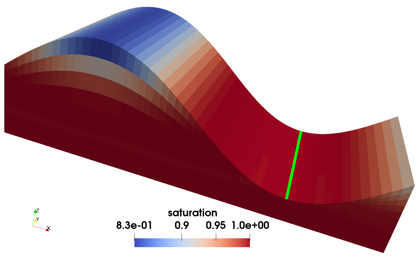
Figure 8: The saturation at steady-state.
Abstracting groundwater
The only modifications to the steady-state input file needed when modelling the abstraction are the reading of the steady-state solution from the steady-state output result, and the inclusion of the abstraction borehole.
Reading the steady-state solution
The steady-state solution is used to initialise the transient simulation. The mesh is read:
[Mesh]
  [from_steady_state]
    type = FileMeshGenerator
    file = gold/ex02_steady_state_ex.e
  []
[]
A SolutionUserObject is employed to read the steady-state solution:
  [steady_state_solution]
    type = SolutionUserObject
    execute_on = INITIAL
    mesh = gold/ex02_steady_state_ex.e
    timestep = LATEST
    system_variables = pp
  []
and the pp Variable is initialized:
[ICs]
  [pp]
    type = FunctionIC
    variable = pp
    function = steady_state_pp
  []
[]
The abstraction borehole
A PorousFlowPeacemanBorehole is used to model the borehole:
  [horizontal_borehole]
    type = PorousFlowPeacemanBorehole
    SumQuantityUO = abstraction
    bottom_p_or_t = -1E5
    unit_weight = '0 0 -1E4'
    character = 1.0
    point_file = ex02.bh
    variable = pp
  []
with point file representing a long horizontal borehole with radius 0.2m at an elevation of -90m that sits almost directly underneath the river (the river sits at , while the borehole is at ):
0.2 240 -200 -90
0.2 240 -190 -90
0.2 240 -180 -90
0.2 240 -170 -90
0.2 240 -160 -90
0.2 240 -150 -90
0.2 240 -140 -90
0.2 240 -130 -90
0.2 240 -120 -90
0.2 240 -110 -90
0.2 240 -100 -90
0.2 240 -90 -90
0.2 240 -80 -90
0.2 240 -70 -90
0.2 240 -60 -90
0.2 240 -50 -90
0.2 240 -40 -90
0.2 240 -30 -90
0.2 240 -20 -90
0.2 240 -10 -90
0.2 240 0 -90
0.2 240 10 -90
0.2 240 20 -90
0.2 240 30 -90
0.2 240 40 -90
0.2 240 50 -90
0.2 240 60 -90
0.2 240 70 -90
0.2 240 80 -90
0.2 240 90 -90
0.2 240 100 -90
0.2 240 110 -90
0.2 240 120 -90
0.2 240 130 -90
0.2 240 140 -90
0.2 240 150 -90
0.2 240 160 -90
0.2 240 170 -90
0.2 240 180 -90
0.2 240 190 -90
0.2 240 200 -90
The value bottom_p_or_t = -1E5 means that the pump at the borehole's bottom point is able to suck at -1atmosphere of pressure. (In this case, the borehole is horizontal, so its "bottom point" is meaningless, but in general it is the first point in the point_file, as explained in the documentation.)
It is vital that readers understand that a PorousFlowPeacemanBorehole uses an approximation of the groundwater solution around a small borehole in order to accurately represent the small borehole in a coarse mesh. The small borehole need not coincide with the finite-element nodes or elements, since the Peaceman formulation automatically takes the mesh into consideration. In this case, it means that the porepressure at any node around the borehole will not be Pa, even though bottom_p_or_t = -1E5. This is in stark contrast to a PorousFlowPolyLineSink, which can easily force the porepressure to be a fixed value at the borehole if the magnitude of fluxes is set high enough. The difference is quantified in a section below. Almost always:
Peaceman boreholes should be used to represent boreholes
PolyLine sinks should be used to represent surface features such as streams and the interaction with the atmosphere, where the stream or atmosphere is sufficiently "huge" that it does actually fix porepressure at the point of interest.
Results
The borehole extracts very little groundwater — only a paltry 7.6litre/day — which is not suprising given its small diameter and the "tightness" of the aquifer. The porepressure in the proximity of the river is only reduced by around 0.2Pa, as shown in Figure 9. This reduces the baseflow from 11.09litre/m/day to 11.07litre/m/day.
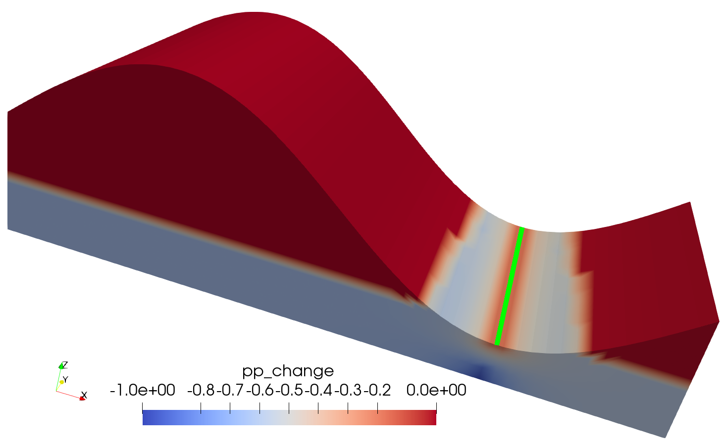
Figure 9: The porepressure change due to groundwater abstraction.
Groundwater modelling therefore suggests that the borehole will have negligible impact on the environment, but will also produce virtually no water.
Using a PolyLineSink
It is a mistake to use a PorousFlowPolyLineSink to represent the borehole in this case, such as
  [polyline_sink_borehole]
    type = PorousFlowPolyLineSink
    SumQuantityUO = abstraction
    fluxes = '-0.4 0 0.4'
    p_or_t_vals = '-1E8 0 1E8'
    point_file = ex02.bh
    variable = pp
If the fluxes parameters were chosen sufficiently large, this would fix the porepressure at finite-element nodes surrounding the borehole to the value of 0Pa. Since the finite-element mesh has a resolution of around , this could correspond to a collosal borehole with cross-sectional size (and length of 400m from the width of the model)!
In this case, the water extracted by the borehole is around 640litre/day, and the river becomes leaky with 4.5litre/m/day of river water entering the groundwater system (and flowing to the borehole). The porepressure change is much larger, as shown in Figure 10.
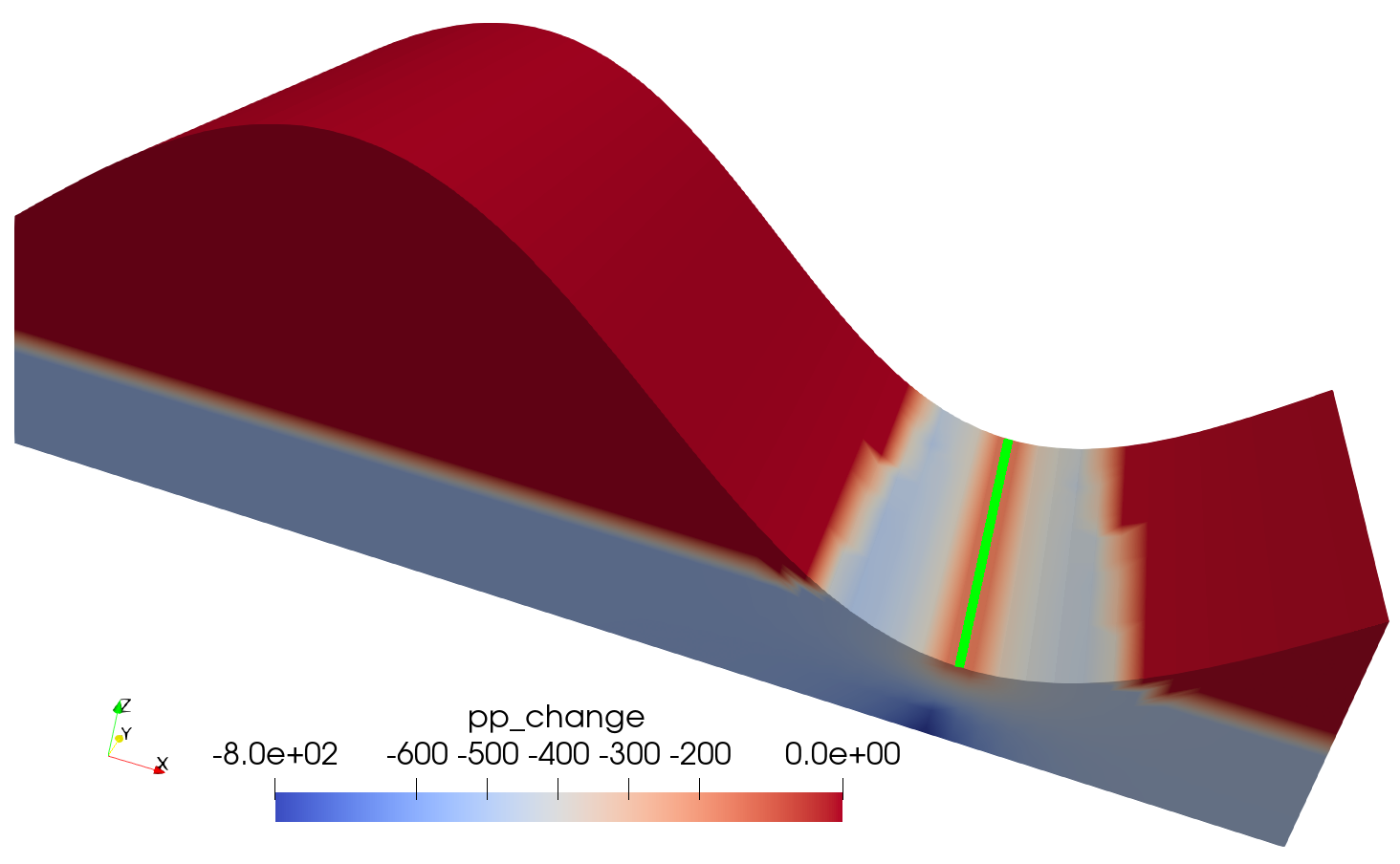
Figure 10: The porepressure change due to groundwater abstraction when erroneously using a PorousFlowPolyLineSink to represent the borehole.
Final words
This page has presented some very simple groundwater models that you can use as a framework to build your realistic models. PorousFlow is highly functional and has been used to solve very complicated groundwater models, but if you require extra functionality not already included, please ask on the MOOSE discussion list.
References
- N. F. Herron, L. Peeters, R. Crosbie, S. P. Marvanek, D. Pagendam, A. Ramage, P. K. Rachakonda, and A. Wilkins.
Groundwater numerical modelling for the Hunter subregion. Product 2.6.2 for the Hunter subregion from the Northern Sydney Basin Bioregional Assessment.
Technical Report, Department of the Environment and Energy, Bureau of Meteorology, CSIRO and Geoscience Australia, Canberra, 2018.
URL: http://data.bioregionalassessments.gov.au/product/NSB/HUN/2.6.2.[BibTeX]