Simulating underground coal mining
Introduction
In an underground longwall coal mine, coal is mined in "panels", as shown in Figure 1. These panels are typically 3–4m in height, 150–400m in width and 1000–4000m long. Coal is extracted from one end, moving towards the other end. As mining progresses, a void is created behind the mining machinery where the coal used to be. The rock material above this void— the "overburden"—is not strong enough to support itself, so it collapses downwards. The resulting partial void and collapsed material is called the "goaf" (or "gob").
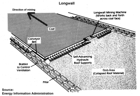
Figure 1: Pictorial representation of a single panel in longwall mining. The dimensions and process are described in the text. Figure sourced from citizensagainstlongwallmining.org who obtained it from the Energy Information Administration.
There are many geotechnical aspects that are of interest in this process, but this Example concentrates on the following.
The vertical displacement of the ground surface due to the longwall mining. This is called the "subsidence". This obviously has effects on buildings and other man-made structures like roads, but it can also change surface water pathways, affect vegetation, and cause surface-water ponding, which all have effects on the local ecology.
The vertical deformation within the overburden.
The patterns of fracture in the overburden. Together with the previous item, this can have effects on operational aspects of longwall mining, such as the load patterns on the "chocks" that support the roof of the goaf next to the mining machinery. It also strongly effects the flow of fluids in the porous rocks that make up the overburden, as discussed next.
The flow of water through the rock. If the fracturing and deformation is extensive then fluids can easily move through the rock. This can result in mines flooding with water, or causing excessive drawdown of groundwater aquifers which can effect other users of groundwater (such as irrigators for farming) or can effect the rates of groundwater baseflow to surrounding river systems which may effect local and not-so-local ecosystems. The deformation and fracture of the overburden can also lead to aquifer mixing, where an aquifer consisting of "dirty" water (with high salinity, for example) pollutes a nearby aquifer of clean water. Although not studied in this Example, the deformation and fracture can also lead to large releases of methane gas from overlying (and underlying) coal seams. This methane can then flow through the highly permeable fractured rock system to the atmosphere, resulting in large greenhouse gas emissions. Or it can flow to the mine workings which is extremely hazardous in terms of mine fires and explosions.
This Example does not seek to build a realistic model of a specific mine. Instead, it explains how the PorousFlow module can be used to build such a model, by exploring a simple 3D model.
The model
Two input files are provided with this example: coarse_with_fluid.i and fine_with_fluid.i. They essentially only differ in the input mesh. The results below are drawn from the fine model, but it takes a few hours to complete on a computer cluster, so the coarse model might be a better model to explore initially.
Geometry
Figure 2 shows the geometrical setup as well as the fine mesh. The model represents a single longwall panel of total width 300m and length 1000m. Only half of the width is modelled, and appropriate boundary conditions used to simulate the full panel. In the fine model, the panel is meshed with 10m square elements.
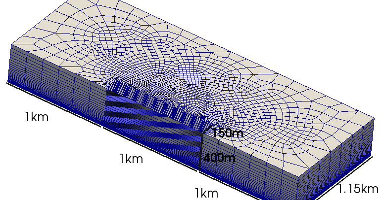
Figure 2: The geometry of the model and the mesh used. A single longwall panel of total width 300m and length 1000m is represented by the region with a fine mesh.
Fluid mechanics
Single-phase unsaturated fluid is used with the nonlinear Variable being the fluid porepressure. Full coupling with mechanical deformations is used, so the Kernels read
  [mass0]
    type = PorousFlowMassTimeDerivative
    fluid_component = 0
    variable = porepressure
  []
  [flux]
    type = PorousFlowAdvectiveFlux
    use_displaced_mesh = false
    variable = porepressure
    gravity = '0 0 -10E-6'
    fluid_component = 0
  []
  [poro_vol_exp]
    type = PorousFlowMassVolumetricExpansion
    block = '2 3 4 5 6 7 8 9 10 11 12 13 14 15 16'
    variable = porepressure
    fluid_component = 0
  []
[]
All stresses are measured in MPa and the time unit is years. A Biot coefficient of 0.7 is used, and the fluid properties are:
[Modules]
  [FluidProperties]
    [simple_fluid]
      type = SimpleFluidProperties
      bulk_modulus = 2E3
      density0 = 1000
      thermal_expansion = 0
      viscosity = 3.5E-17
    []
  []
[]
A van Genuchten capillary pressure relationship is used
  [pc]
    type = PorousFlowCapillaryPressureVG
    m = 0.5
    alpha = 1 # MPa^-1
  []
A Corey relative permeability is used
  [relperm]
    type = PorousFlowRelativePermeabilityCorey
    n = 4
    s_res = 0.4
    sum_s_res = 0.4
    phase = 0
  []
The fluid porepressure is fixed at the outer boundaries, and a PorousFlowPiecewiseLinearSink with a spatially and temporally varying flux_function is used to withdraw water from the rock into the goaf:
  [fix_porepressure]
    type = FunctionDirichletBC
    variable = porepressure
    boundary = 'ymin ymax xmax'
    function = ini_pp
  []
  [roof_porepressure]
    type = PorousFlowPiecewiseLinearSink
    variable = porepressure
    pt_vals = '-1E3 1E3'
    multipliers = '-1 1'
    fluid_phase = 0
    flux_function = roof_conductance
    boundary = roof
  []
In multi-phase scenarios, such a simple representation of the goaf boundary condition is not valid.
Solid mechanics
Layered Cosserat solid mechanics is employed, meaning there are 3 translational and 2 rotational degrees of freedom. A quasi-static approximation is used, so the solid-mechanical Kernels are
  [cx_elastic]
    type = CosseratStressDivergenceTensors
    use_displaced_mesh = false
    variable = disp_x
    component = 0
  []
  [cy_elastic]
    type = CosseratStressDivergenceTensors
    use_displaced_mesh = false
    variable = disp_y
    component = 1
  []
  [cz_elastic]
    type = CosseratStressDivergenceTensors
    use_displaced_mesh = false
    variable = disp_z
    component = 2
  []
  [x_couple]
    type = StressDivergenceTensors
    use_displaced_mesh = false
    variable = wc_x
    displacements = 'wc_x wc_y wc_z'
    component = 0
    base_name = couple
  []
  [y_couple]
    type = StressDivergenceTensors
    use_displaced_mesh = false
    variable = wc_y
    displacements = 'wc_x wc_y wc_z'
    component = 1
    base_name = couple
  []
  [x_moment]
    type = MomentBalancing
    use_displaced_mesh = false
    variable = wc_x
    component = 0
  []
  [y_moment]
    type = MomentBalancing
    use_displaced_mesh = false
    variable = wc_y
    component = 1
  []
  [gravity]
    type = Gravity
    use_displaced_mesh = false
    variable = disp_z
    value = -10E-6 # remember this is in MPa
  []
  [poro_x]
    type = PorousFlowEffectiveStressCoupling
    use_displaced_mesh = false
    variable = disp_x
    component = 0
  []
  [poro_y]
    type = PorousFlowEffectiveStressCoupling
    use_displaced_mesh = false
    variable = disp_y
    component = 1
  []
  [poro_z]
    type = PorousFlowEffectiveStressCoupling
    use_displaced_mesh = false
    component = 2
    variable = disp_z
  []
Quite a complicated elasto-plastic model is used and this accounts for the majority of nonlinear iterations of this model, as well as the relative slowness of computing the residual and Jacobian. The elasticity tensors (one for standard, one for Cosserat) are computed via:
  [elasticity_tensor_0]
    type = ComputeLayeredCosseratElasticityTensor
     block = '2 3 4 5 6 7 8 9 10 11 12 13 14 15 16'
    young = 8E3 # MPa
    poisson = 0.25
    layer_thickness = 1.0
    joint_normal_stiffness = 1E9 # huge
    joint_shear_stiffness = 1E3 # MPa
  []
  [elasticity_tensor_1]
    type = ComputeLayeredCosseratElasticityTensor
    block = 1
    young = 8E3 # MPa
    poisson = 0.25
    layer_thickness = 1.0
    joint_normal_stiffness = 1E9 # huge
    joint_shear_stiffness = 1E3 # MPa
    elasticity_tensor_prefactor = excav_sideways
  []
where the excav_sideways Function simulates the excavation of coal (it is 1 ahead of the coal face and zero behind it). Small strain is used, and an insitu stress that increases with depth is assumed:
  [strain]
    type = ComputeCosseratIncrementalSmallStrain
    eigenstrain_names = ini_stress
  []
  [ini_stress]
    type = ComputeEigenstrainFromInitialStress
    eigenstrain_name = ini_stress
    initial_stress = 'ini_xx 0 0  0 ini_xx 0  0 0 ini_zz'
  []
Capped Mohr-Coulomb plus weak-plane plasticity is used and the plastic models are cycled
  [stress_0]
    type = ComputeMultipleInelasticCosseratStress
     block = '2 3 4 5 6 7 8 9 10 11 12 13 14 15 16'
    inelastic_models = 'mc wp'
    cycle_models = true
    relative_tolerance = 2.0
    absolute_tolerance = 1E6
    max_iterations = 1
    tangent_operator = nonlinear
    perform_finite_strain_rotations = false
  []
  [stress_1]
    type = ComputeMultipleInelasticCosseratStress
    block = 1
    inelastic_models = ''
    relative_tolerance = 2.0
    absolute_tolerance = 1E6
    max_iterations = 1
    tangent_operator = nonlinear
    perform_finite_strain_rotations = false
  []
  [mc]
    type = CappedMohrCoulombCosseratStressUpdate
    warn_about_precision_loss = false
    host_youngs_modulus = 8E3
    host_poissons_ratio = 0.25
    base_name = mc
    tensile_strength = mc_tensile_str_strong_harden
    compressive_strength = mc_compressive_str
    cohesion = mc_coh_strong_harden
    friction_angle = mc_fric
    dilation_angle = mc_dil
    max_NR_iterations = 100000
    smoothing_tol = 0.1 # MPa  # Must be linked to cohesion
    yield_function_tol = 1E-9 # MPa.  this is essentially the lowest possible without lots of precision loss
    perfect_guess = true
    min_step_size = 1.0
  []
  [wp]
    type = CappedWeakPlaneCosseratStressUpdate
    warn_about_precision_loss = false
    base_name = wp
    cohesion = wp_coh_harden
    tan_friction_angle = wp_tan_fric
    tan_dilation_angle = wp_tan_dil
    tensile_strength = wp_tensile_str_harden
    compressive_strength = wp_compressive_str_soften
    max_NR_iterations = 10000
    tip_smoother = 0.05
    smoothing_tol = 0.05 # MPa  # Note, this must be tied to cohesion, otherwise get no possible return at cone apex
    yield_function_tol = 1E-11 # MPa.  this is essentially the lowest possible without lots of precision loss
    perfect_guess = true
    min_step_size = 1.0E-3
  []
The plastic moduli are:
  [mc_coh_strong_harden]
    type = TensorMechanicsHardeningExponential
    value_0 = 1.99 # MPa
    value_residual = 2.01 # MPa
    rate = 1.0
  []
  [mc_fric]
    type = TensorMechanicsHardeningConstant
    value = 0.61 # 35deg
  []
  [mc_dil]
    type = TensorMechanicsHardeningConstant
    value = 0.15 # 8deg
  []

  [mc_tensile_str_strong_harden]
    type = TensorMechanicsHardeningExponential
    value_0 = 1.0 # MPa
    value_residual = 1.0 # MPa
    rate = 1.0
  []
  [mc_compressive_str]
    type = TensorMechanicsHardeningCubic
    value_0 = 100 # Large!
    value_residual = 100
    internal_limit = 0.1
  []

  [wp_coh_harden]
    type = TensorMechanicsHardeningCubic
    value_0 = 0.05
    value_residual = 0.05
    internal_limit = 10
  []
  [wp_tan_fric]
    type = TensorMechanicsHardeningConstant
    value = 0.26 # 15deg
  []
  [wp_tan_dil]
    type = TensorMechanicsHardeningConstant
    value = 0.18 # 10deg
  []

  [wp_tensile_str_harden]
    type = TensorMechanicsHardeningCubic
    value_0 = 0.05
    value_residual = 0.05
    internal_limit = 10
  []
  [wp_compressive_str_soften]
    type = TensorMechanicsHardeningCubic
    value_0 = 100
    value_residual = 1
    internal_limit = 1.0
  []
[]
Roller boundary conditions are prescribed at the boundaries. At the roof of the excavation, a StickyBC is employed to prevent the roof from collapsing further than 3m:
  [roof_bcs]
    type = StickyBC
    variable = disp_z
    min_value = -3.0
    boundary = roof
Coupling
Full coupling between the fluid and solid mechanics is evident in the Kernels. The PorousFlowDictator ensures all nonzero Jacobian entries are computed:
  [dictator]
    type = PorousFlowDictator
    porous_flow_vars = 'porepressure disp_x disp_y disp_z'
    number_fluid_phases = 1
    number_fluid_components = 1
  []
Other aspects of the fluid-solid coupling are the porosity:
  [porosity_bulk]
    type = PorousFlowPorosity
    fluid = true
    mechanical = true
    block = '2 3 4 5 6 7 8 9 10 11 12 13 14 15 16'
    ensure_positive = true
    porosity_zero = 0.02
    solid_bulk = 5.3333E3
  []
and the permeability:
  [permeability_bulk]
    type = PorousFlowPermeabilityKozenyCarman
    block = '2 3 4 5 6 7 8 9 10 11 12 13 14 15 16'
    poroperm_function = kozeny_carman_phi0
    k0 = 1E-15
    phi0 = 0.02
    n = 2
    m = 2
  []
Results
Despite being a very simple model with no interesting lithology that usually induces characteristic fracture and displacement patterns, the results display many interesting features.
Figure 3: The evolution of the destressed zone where the vertical stress has less magnitude than the initial vertical stress. The zone is colored by the magnitude of de-stressing. The black rectangle shows the coal that will be excavated.
Figure 4: The evolution of the zone where the vertical displacement is cm. The zone is colored by the magnitude of vertical displacement. The black rectangle shows the coal that will be excavated.
Figure 5: The evolution of the zone where the porepressure is reduced by more than MPa. The zone is colored by the magnitude of the porepressure reduction. The green arrows show the Darcy velocity. The black rectangle shows the coal that will be excavated.
Some of interesting features are:
Initially the roof holds up before suddenly collapsing at around 100m of excavation.
After this point, there is some periodicity in the plastic strains and vertical stresses, although this may be an artificat of the mesh rather than anything physical.
The minimum vertical displacement is actually m in the region where the sudden collapse occurs towards the start of the panel. The StickyBC are not sufficient to prevent this. Therefore, the results towards the panel's beginning shouldn't be treated too seriously. To avoid this, MOOSE's Constraint system, or the mining-specific features CSIRO's private MOOSE-based app, could be employed.
There is significant rock fracture, indicated by the Mohr-Coulomb plastic strains of greater than % in the immediate 10m of the roof.
Mohr-Coulomb shear failure is much more prevelant than Mohr-Coulomb tensile failure throughout the model.
Mohr-Coulomb shear failure also occurs in the unexcavated material close to the panel (the ribs and roadways).
Tensile opening of the joints occurs in large regions of the roof, indicated by weak-plane tensile plasticity of greater than %.
Shear failure of the joints occurs throughout all regions of the model above the goaf. It is greater than 1% in the immediate m of the roof.
The surrounding unexcavated material experiences large vertical loads, while there is an annular region on the outside and above the excavation that is de-stressed. The material above the goaf therefore experiences de-stressing and then recompaction.
Porosity and permeability enhancement typically occurs in regions of highest weak-plane failure. The permeability is increased by approximately a factor of 2 in the goaf region. This is actually a tiny enhancement compared to the expected value of around and is due to the Kozeny-Carman permeability relationship which is not really valid in this setting. If readers are interested in simulating realistic mining-induced permeability enhancements they should enquire about using CSIRO's private MOOSE-based app.
Mining-induced drawdown of the water porepressure at the ground surface starts to occur after around m (2 weeks) of excavation. In this model, the region above the panel rapidly becomes unsaturated, with saturation reaching approximately 80%, as water flows to the goaf region.
Most of the high Darcy fluid velocities occur around the periphery of the mining panel.
Results along the centre-line of the panel.
The figures below show results contoured on a vertical section along the centre-line of the panel, after excavation has completed. The excavation is shown as a black line.
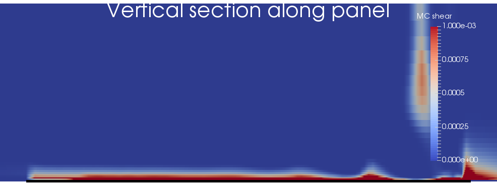
Mohr-Coulomb shear plastic strain on a vertical section along the centre-line of the panel
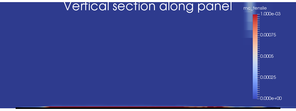
Mohr-Coulomb tensile plastic strain on a vertical section along the centre-line of the panel
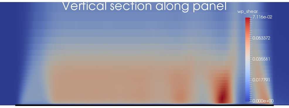
Weak-plane shear plastic strain on a vertical section along the centre-line of the panel
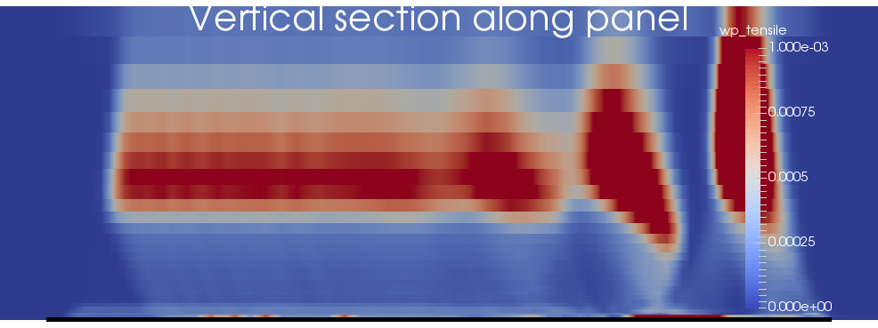
Weak-plane tensile plastic strain on a vertical section along the centre-line of the panel
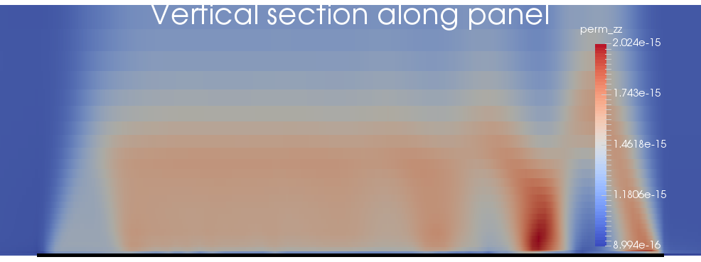
Vertical permeability on a vertical section along the centre-line of the panel
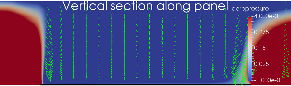
Porepressure (color) and Darcy flow vectors on a vertical section along the centre-line of the panel
Results across the panel.
The figures below show results contoured on a vertical section across the half-panel that is modelled, after excavation has completed. The excavation is shown as a black line.
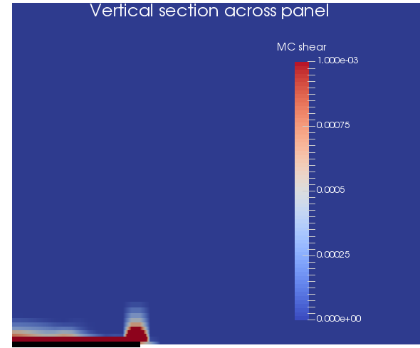
Mohr-Coulomb shear plastic strain on a vertical section across the panel
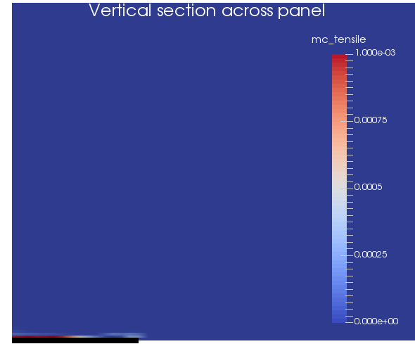
Mohr-Coulomb tensile plastic strain on a vertical section across the panel
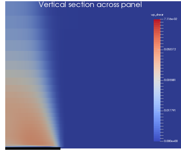
Weak-plane shear plastic strain on a vertical section across the panel
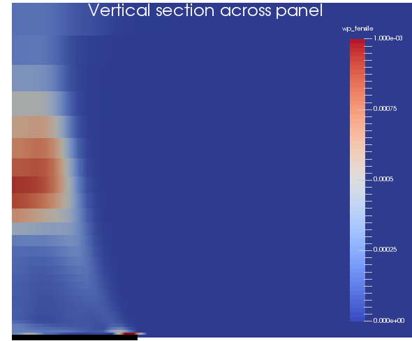
Weak-plane tensile plastic strain on a vertical section across the panel
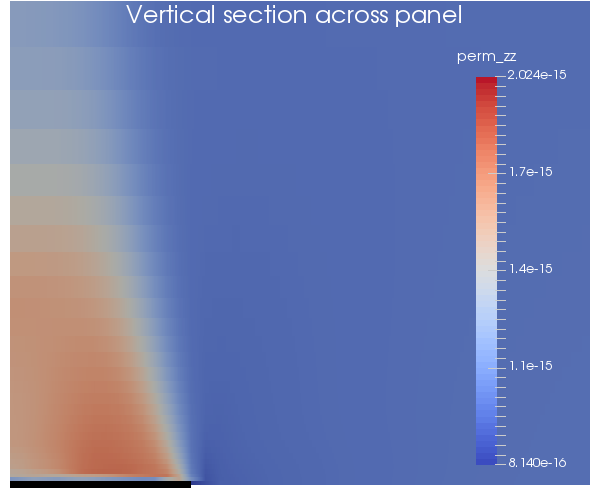
Vertical permeability on a vertical section across the panel
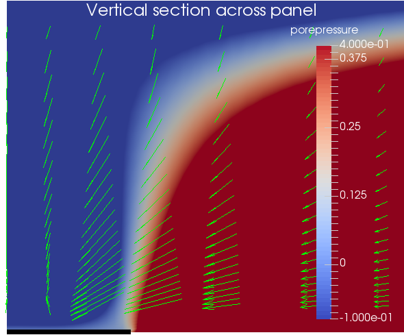
Porepressure (color) and Darcy flow vectors on a vertical section across the panel
(modules/porous_flow/examples/coal_mining/coarse_with_fluid.i)
# Strata deformation and fluid flow aaround a coal mine - 3D model
#
# A "half model" is used.  The mine is 400m deep and
# just the roof is studied (-400<=z<=0).  The mining panel
# sits between 0<=x<=150, and 0<=y<=1000, so this simulates
# a coal panel that is 300m wide and 1000m long.  The outer boundaries
# are 1km from the excavation boundaries.
#
# The excavation takes 0.5 years.
#
# The boundary conditions for this simulation are:
#  - disp_x = 0 at x=0 and x=1150
#  - disp_y = 0 at y=-1000 and y=1000
#  - disp_z = 0 at z=-400, but there is a time-dependent
#               Young modulus that simulates excavation
#  - wc_x = 0 at y=-1000 and y=1000
#  - wc_y = 0 at x=0 and x=1150
#  - no flow at x=0, z=-400 and z=0
#  - fixed porepressure at y=-1000, y=1000 and x=1150
# That is, rollers on the sides, free at top,
# and prescribed at bottom in the unexcavated portion.
#
# A single-phase unsaturated fluid is used.
#
# The small strain formulation is used.
#
# All stresses are measured in MPa, and time units are measured in years.
#
# The initial porepressure is hydrostatic with P=0 at z=0, so
# Porepressure ~ - 0.01*z MPa, where the fluid has density 1E3 kg/m^3 and
# gravity = = 10 m.s^-2 = 1E-5 MPa m^2/kg.
# To be more accurate, i use
# Porepressure = -bulk * log(1 + g*rho0*z/bulk)
# where bulk=2E3 MPa and rho0=1Ee kg/m^3.
# The initial stress is consistent with the weight force from undrained
# density 2500 kg/m^3, and fluid porepressure, and a Biot coefficient of 0.7, ie,
# stress_zz^effective = 0.025*z + 0.7 * initial_porepressure
# The maximum and minimum principal horizontal effective stresses are
# assumed to be equal to 0.8*stress_zz.
#
# Material properties:
# Young's modulus = 8 GPa
# Poisson's ratio = 0.25
# Cosserat layer thickness = 1 m
# Cosserat-joint normal stiffness = large
# Cosserat-joint shear stiffness = 1 GPa
# MC cohesion = 2 MPa
# MC friction angle = 35 deg
# MC dilation angle = 8 deg
# MC tensile strength = 1 MPa
# MC compressive strength = 100 MPa
# WeakPlane cohesion = 0.1 MPa
# WeakPlane friction angle = 30 deg
# WeakPlane dilation angle = 10 deg
# WeakPlane tensile strength = 0.1 MPa
# WeakPlane compressive strength = 100 MPa softening to 1 MPa at strain = 1
# Fluid density at zero porepressure = 1E3 kg/m^3
# Fluid bulk modulus = 2E3 MPa
# Fluid viscosity = 1.1E-3 Pa.s = 1.1E-9 MPa.s = 3.5E-17 MPa.year
#
[GlobalParams]
  perform_finite_strain_rotations = false
  displacements = 'disp_x disp_y disp_z'
  Cosserat_rotations = 'wc_x wc_y wc_z'
  PorousFlowDictator = dictator
  biot_coefficient = 0.7
[]

[Mesh]
  [file]
    type = FileMeshGenerator
    file = mesh/coarse.e
  []
  [xmin]
    type = SideSetsAroundSubdomainGenerator
     block = '2 3 4 5 6 7 8 9 10 11 12 13 14 15 16'
    new_boundary = xmin
    normal = '-1 0 0'
    input = file
  []
  [xmax]
    type = SideSetsAroundSubdomainGenerator
     block = '2 3 4 5 6 7 8 9 10 11 12 13 14 15 16'
    new_boundary = xmax
    normal = '1 0 0'
    input = xmin
  []
  [ymin]
    type = SideSetsAroundSubdomainGenerator
     block = '2 3 4 5 6 7 8 9 10 11 12 13 14 15 16'
    new_boundary = ymin
    normal = '0 -1 0'
    input = xmax
  []
  [ymax]
    type = SideSetsAroundSubdomainGenerator
     block = '2 3 4 5 6 7 8 9 10 11 12 13 14 15 16'
    new_boundary = ymax
    normal = '0 1 0'
    input = ymin
  []
  [zmax]
    type = SideSetsAroundSubdomainGenerator
    block = 16
    new_boundary = zmax
    normal = '0 0 1'
    input = ymax
  []
  [zmin]
    type = SideSetsAroundSubdomainGenerator
    block = 2
    new_boundary = zmin
    normal = '0 0 -1'
    input = zmax
  []
  [excav]
    type = SubdomainBoundingBoxGenerator
    input = zmin
    block_id = 1
    bottom_left = '0 0 -400'
    top_right = '150 1000 -397'
  []
  [roof]
    type = SideSetsBetweenSubdomainsGenerator
    primary_block = 3
    paired_block = 1
    input = excav
    new_boundary = roof
  []
[]

[Variables]
  [disp_x]
  []
  [disp_y]
  []
  [disp_z]
  []
  [wc_x]
  []
  [wc_y]
  []
  [porepressure]
    scaling = 1E-5
  []
[]

[ICs]
  [porepressure]
    type = FunctionIC
    variable = porepressure
    function = ini_pp
  []
[]

[Kernels]
  [cx_elastic]
    type = CosseratStressDivergenceTensors
    use_displaced_mesh = false
    variable = disp_x
    component = 0
  []
  [cy_elastic]
    type = CosseratStressDivergenceTensors
    use_displaced_mesh = false
    variable = disp_y
    component = 1
  []
  [cz_elastic]
    type = CosseratStressDivergenceTensors
    use_displaced_mesh = false
    variable = disp_z
    component = 2
  []
  [x_couple]
    type = StressDivergenceTensors
    use_displaced_mesh = false
    variable = wc_x
    displacements = 'wc_x wc_y wc_z'
    component = 0
    base_name = couple
  []
  [y_couple]
    type = StressDivergenceTensors
    use_displaced_mesh = false
    variable = wc_y
    displacements = 'wc_x wc_y wc_z'
    component = 1
    base_name = couple
  []
  [x_moment]
    type = MomentBalancing
    use_displaced_mesh = false
    variable = wc_x
    component = 0
  []
  [y_moment]
    type = MomentBalancing
    use_displaced_mesh = false
    variable = wc_y
    component = 1
  []
  [gravity]
    type = Gravity
    use_displaced_mesh = false
    variable = disp_z
    value = -10E-6 # remember this is in MPa
  []
  [poro_x]
    type = PorousFlowEffectiveStressCoupling
    use_displaced_mesh = false
    variable = disp_x
    component = 0
  []
  [poro_y]
    type = PorousFlowEffectiveStressCoupling
    use_displaced_mesh = false
    variable = disp_y
    component = 1
  []
  [poro_z]
    type = PorousFlowEffectiveStressCoupling
    use_displaced_mesh = false
    component = 2
    variable = disp_z
  []
  [mass0]
    type = PorousFlowMassTimeDerivative
    fluid_component = 0
    variable = porepressure
  []
  [flux]
    type = PorousFlowAdvectiveFlux
    use_displaced_mesh = false
    variable = porepressure
    gravity = '0 0 -10E-6'
    fluid_component = 0
  []
  [poro_vol_exp]
    type = PorousFlowMassVolumetricExpansion
    block = '2 3 4 5 6 7 8 9 10 11 12 13 14 15 16'
    variable = porepressure
    fluid_component = 0
  []
[]


[AuxVariables]
  [saturation]
    order = CONSTANT
    family = MONOMIAL
  []
  [darcy_x]
    order = CONSTANT
    family = MONOMIAL
  []
  [darcy_y]
    order = CONSTANT
    family = MONOMIAL
  []
  [darcy_z]
    order = CONSTANT
    family = MONOMIAL
  []
  [porosity]
    order = CONSTANT
    family = MONOMIAL
  []
  [wc_z]
  []
  [stress_xx]
    order = CONSTANT
    family = MONOMIAL
  []
  [stress_xy]
    order = CONSTANT
    family = MONOMIAL
  []
  [stress_xz]
    order = CONSTANT
    family = MONOMIAL
  []
  [stress_yx]
    order = CONSTANT
    family = MONOMIAL
  []
  [stress_yy]
    order = CONSTANT
    family = MONOMIAL
  []
  [stress_yz]
    order = CONSTANT
    family = MONOMIAL
  []
  [stress_zx]
    order = CONSTANT
    family = MONOMIAL
  []
  [stress_zy]
    order = CONSTANT
    family = MONOMIAL
  []
  [stress_zz]
    order = CONSTANT
    family = MONOMIAL
  []
  [total_strain_xx]
    order = CONSTANT
    family = MONOMIAL
  []
  [total_strain_xy]
    order = CONSTANT
    family = MONOMIAL
  []
  [total_strain_xz]
    order = CONSTANT
    family = MONOMIAL
  []
  [total_strain_yx]
    order = CONSTANT
    family = MONOMIAL
  []
  [total_strain_yy]
    order = CONSTANT
    family = MONOMIAL
  []
  [total_strain_yz]
    order = CONSTANT
    family = MONOMIAL
  []
  [total_strain_zx]
    order = CONSTANT
    family = MONOMIAL
  []
  [total_strain_zy]
    order = CONSTANT
    family = MONOMIAL
  []
  [total_strain_zz]
    order = CONSTANT
    family = MONOMIAL
  []
  [perm_xx]
    order = CONSTANT
    family = MONOMIAL
  []
  [perm_yy]
    order = CONSTANT
    family = MONOMIAL
  []
  [perm_zz]
    order = CONSTANT
    family = MONOMIAL
  []
  [mc_shear]
    order = CONSTANT
    family = MONOMIAL
  []
  [mc_tensile]
    order = CONSTANT
    family = MONOMIAL
  []
  [wp_shear]
    order = CONSTANT
    family = MONOMIAL
  []
  [wp_tensile]
    order = CONSTANT
    family = MONOMIAL
  []
  [wp_shear_f]
    order = CONSTANT
    family = MONOMIAL
  []
  [wp_tensile_f]
    order = CONSTANT
    family = MONOMIAL
  []
  [mc_shear_f]
    order = CONSTANT
    family = MONOMIAL
  []
  [mc_tensile_f]
    order = CONSTANT
    family = MONOMIAL
  []
[]

[AuxKernels]
  [saturation_water]
    type = PorousFlowPropertyAux
    variable = saturation
    property = saturation
    phase = 0
    execute_on = timestep_end
  []
  [darcy_x]
    type = PorousFlowDarcyVelocityComponent
    variable = darcy_x
    gravity = '0 0 -10E-6'
    component = x
  []
  [darcy_y]
    type = PorousFlowDarcyVelocityComponent
    variable = darcy_y
    gravity = '0 0 -10E-6'
    component = y
  []
  [darcy_z]
    type = PorousFlowDarcyVelocityComponent
    variable = darcy_z
    gravity = '0 0 -10E-6'
    component = z
  []
  [porosity]
    type = PorousFlowPropertyAux
    property = porosity
    variable = porosity
    execute_on = timestep_end
  []
  [stress_xx]
    type = RankTwoAux
    rank_two_tensor = stress
    variable = stress_xx
    index_i = 0
    index_j = 0
    execute_on = timestep_end
  []
  [stress_xy]
    type = RankTwoAux
    rank_two_tensor = stress
    variable = stress_xy
    index_i = 0
    index_j = 1
    execute_on = timestep_end
  []
  [stress_xz]
    type = RankTwoAux
    rank_two_tensor = stress
    variable = stress_xz
    index_i = 0
    index_j = 2
    execute_on = timestep_end
  []
  [stress_yx]
    type = RankTwoAux
    rank_two_tensor = stress
    variable = stress_yx
    index_i = 1
    index_j = 0
    execute_on = timestep_end
  []
  [stress_yy]
    type = RankTwoAux
    rank_two_tensor = stress
    variable = stress_yy
    index_i = 1
    index_j = 1
    execute_on = timestep_end
  []
  [stress_yz]
    type = RankTwoAux
    rank_two_tensor = stress
    variable = stress_yz
    index_i = 1
    index_j = 2
    execute_on = timestep_end
  []
  [stress_zx]
    type = RankTwoAux
    rank_two_tensor = stress
    variable = stress_zx
    index_i = 2
    index_j = 0
    execute_on = timestep_end
  []
  [stress_zy]
    type = RankTwoAux
    rank_two_tensor = stress
    variable = stress_zy
    index_i = 2
    index_j = 1
    execute_on = timestep_end
  []
  [stress_zz]
    type = RankTwoAux
    rank_two_tensor = stress
    variable = stress_zz
    index_i = 2
    index_j = 2
    execute_on = timestep_end
  []
  [total_strain_xx]
    type = RankTwoAux
    rank_two_tensor = total_strain
    variable = total_strain_xx
    index_i = 0
    index_j = 0
    execute_on = timestep_end
  []
  [total_strain_xy]
    type = RankTwoAux
    rank_two_tensor = total_strain
    variable = total_strain_xy
    index_i = 0
    index_j = 1
    execute_on = timestep_end
  []
  [total_strain_xz]
    type = RankTwoAux
    rank_two_tensor = total_strain
    variable = total_strain_xz
    index_i = 0
    index_j = 2
    execute_on = timestep_end
  []
  [total_strain_yx]
    type = RankTwoAux
    rank_two_tensor = total_strain
    variable = total_strain_yx
    index_i = 1
    index_j = 0
    execute_on = timestep_end
  []
  [total_strain_yy]
    type = RankTwoAux
    rank_two_tensor = total_strain
    variable = total_strain_yy
    index_i = 1
    index_j = 1
    execute_on = timestep_end
  []
  [total_strain_yz]
    type = RankTwoAux
    rank_two_tensor = total_strain
    variable = total_strain_yz
    index_i = 1
    index_j = 2
    execute_on = timestep_end
  []
  [total_strain_zx]
    type = RankTwoAux
    rank_two_tensor = total_strain
    variable = total_strain_zx
    index_i = 2
    index_j = 0
    execute_on = timestep_end
  []
  [total_strain_zy]
    type = RankTwoAux
    rank_two_tensor = total_strain
    variable = total_strain_zy
    index_i = 2
    index_j = 1
    execute_on = timestep_end
  []
  [total_strain_zz]
    type = RankTwoAux
    rank_two_tensor = total_strain
    variable = total_strain_zz
    index_i = 2
    index_j = 2
    execute_on = timestep_end
  []
  [perm_xx]
    type = PorousFlowPropertyAux
    property = permeability
    variable = perm_xx
    row = 0
    column = 0
    execute_on = timestep_end
  []
  [perm_yy]
    type = PorousFlowPropertyAux
    property = permeability
    variable = perm_yy
    row = 1
    column = 1
    execute_on = timestep_end
  []
  [perm_zz]
    type = PorousFlowPropertyAux
    property = permeability
    variable = perm_zz
    row = 2
    column = 2
    execute_on = timestep_end
  []
  [mc_shear]
    type = MaterialStdVectorAux
    index = 0
    property = mc_plastic_internal_parameter
    variable = mc_shear
    execute_on = timestep_end
  []
  [mc_tensile]
    type = MaterialStdVectorAux
    index = 1
    property = mc_plastic_internal_parameter
    variable = mc_tensile
    execute_on = timestep_end
  []
  [wp_shear]
    type = MaterialStdVectorAux
    index = 0
    property = wp_plastic_internal_parameter
    variable = wp_shear
    execute_on = timestep_end
  []
  [wp_tensile]
    type = MaterialStdVectorAux
    index = 1
    property = wp_plastic_internal_parameter
    variable = wp_tensile
    execute_on = timestep_end
  []
  [mc_shear_f]
    type = MaterialStdVectorAux
    index = 6
    property = mc_plastic_yield_function
    variable = mc_shear_f
    execute_on = timestep_end
  []
  [mc_tensile_f]
    type = MaterialStdVectorAux
    index = 0
    property = mc_plastic_yield_function
    variable = mc_tensile_f
    execute_on = timestep_end
  []
  [wp_shear_f]
    type = MaterialStdVectorAux
    index = 0
    property = wp_plastic_yield_function
    variable = wp_shear_f
    execute_on = timestep_end
  []
  [wp_tensile_f]
    type = MaterialStdVectorAux
    index = 1
    property = wp_plastic_yield_function
    variable = wp_tensile_f
    execute_on = timestep_end
  []
[]


[BCs]
  [no_x]
    type = DirichletBC
    variable = disp_x
    boundary = 'xmin xmax'
    value = 0.0
  []
  [no_y]
    type = DirichletBC
    variable = disp_y
    boundary = 'ymin ymax'
    value = 0.0
  []
  [no_z]
    type = DirichletBC
    variable = disp_z
    boundary = zmin
    value = 0.0
  []
  [no_wc_x]
    type = DirichletBC
    variable = wc_x
    boundary = 'ymin ymax'
    value = 0.0
  []
  [no_wc_y]
    type = DirichletBC
    variable = wc_y
    boundary = 'xmin xmax'
    value = 0.0
  []
  [fix_porepressure]
    type = FunctionDirichletBC
    variable = porepressure
    boundary = 'ymin ymax xmax'
    function = ini_pp
  []
  [roof_porepressure]
    type = PorousFlowPiecewiseLinearSink
    variable = porepressure
    pt_vals = '-1E3 1E3'
    multipliers = '-1 1'
    fluid_phase = 0
    flux_function = roof_conductance
    boundary = roof
  []
  [roof_bcs]
    type = StickyBC
    variable = disp_z
    min_value = -3.0
    boundary = roof
  []
[]

[Functions]
  [ini_pp]
    type = ParsedFunction
    vars = 'bulk p0 g    rho0'
    vals = '2E3 0.0 1E-5 1E3'
    value = '-bulk*log(exp(-p0/bulk)+g*rho0*z/bulk)'
  []
  [ini_xx]
    type = ParsedFunction
    vars = 'bulk p0 g    rho0 biot'
    vals = '2E3 0.0 1E-5 1E3  0.7'
    value = '0.8*(2500*10E-6*z+biot*(-bulk*log(exp(-p0/bulk)+g*rho0*z/bulk)))'
  []
  [ini_zz]
    type = ParsedFunction
    vars = 'bulk p0 g    rho0 biot'
    vals = '2E3 0.0 1E-5 1E3  0.7'
    value = '2500*10E-6*z+biot*(-bulk*log(exp(-p0/bulk)+g*rho0*z/bulk))'
  []
  [excav_sideways]
    type = ParsedFunction
    vars = 'end_t ymin ymax  minval maxval slope'
    vals = '0.5   0    1000.0 1E-9 1 60'
    # excavation face at ymin+(ymax-ymin)*min(t/end_t,1)
    # slope is the distance over which the modulus reduces from maxval to minval
    value = 'if(y<ymin+(ymax-ymin)*min(t/end_t,1),minval,if(y<ymin+(ymax-ymin)*min(t/end_t,1)+slope,minval+(maxval-minval)*(y-(ymin+(ymax-ymin)*min(t/end_t,1)))/slope,maxval))'
  []
  [density_sideways]
    type = ParsedFunction
    vars = 'end_t ymin ymax  minval maxval'
    vals = '0.5   0    1000.0 0 2500'
    value = 'if(y<ymin+(ymax-ymin)*min(t/end_t,1),minval,maxval)'
  []
  [roof_conductance]
    type = ParsedFunction
    vars = 'end_t ymin ymax   maxval minval'
    vals = '0.5   0    1000.0 1E7      0'
    value = 'if(y<ymin+(ymax-ymin)*min(t/end_t,1),maxval,minval)'
  []
[]

[UserObjects]
  [dictator]
    type = PorousFlowDictator
    porous_flow_vars = 'porepressure disp_x disp_y disp_z'
    number_fluid_phases = 1
    number_fluid_components = 1
  []
  [pc]
    type = PorousFlowCapillaryPressureVG
    m = 0.5
    alpha = 1 # MPa^-1
  []

  [mc_coh_strong_harden]
    type = TensorMechanicsHardeningExponential
    value_0 = 1.99 # MPa
    value_residual = 2.01 # MPa
    rate = 1.0
  []
  [mc_fric]
    type = TensorMechanicsHardeningConstant
    value = 0.61 # 35deg
  []
  [mc_dil]
    type = TensorMechanicsHardeningConstant
    value = 0.15 # 8deg
  []

  [mc_tensile_str_strong_harden]
    type = TensorMechanicsHardeningExponential
    value_0 = 1.0 # MPa
    value_residual = 1.0 # MPa
    rate = 1.0
  []
  [mc_compressive_str]
    type = TensorMechanicsHardeningCubic
    value_0 = 100 # Large!
    value_residual = 100
    internal_limit = 0.1
  []

  [wp_coh_harden]
    type = TensorMechanicsHardeningCubic
    value_0 = 0.05
    value_residual = 0.05
    internal_limit = 10
  []
  [wp_tan_fric]
    type = TensorMechanicsHardeningConstant
    value = 0.26 # 15deg
  []
  [wp_tan_dil]
    type = TensorMechanicsHardeningConstant
    value = 0.18 # 10deg
  []

  [wp_tensile_str_harden]
    type = TensorMechanicsHardeningCubic
    value_0 = 0.05
    value_residual = 0.05
    internal_limit = 10
  []
  [wp_compressive_str_soften]
    type = TensorMechanicsHardeningCubic
    value_0 = 100
    value_residual = 1
    internal_limit = 1.0
  []
[]

[Modules]
  [FluidProperties]
    [simple_fluid]
      type = SimpleFluidProperties
      bulk_modulus = 2E3
      density0 = 1000
      thermal_expansion = 0
      viscosity = 3.5E-17
    []
  []
[]

[Materials]
  [temperature]
    type = PorousFlowTemperature
  []
  [eff_fluid_pressure]
    type = PorousFlowEffectiveFluidPressure
  []
  [vol_strain]
    type = PorousFlowVolumetricStrain
  []
  [ppss]
    type = PorousFlow1PhaseP
    porepressure = porepressure
    capillary_pressure = pc
  []
  [massfrac]
    type = PorousFlowMassFraction
  []
  [simple_fluid]
    type = PorousFlowSingleComponentFluid
    fp = simple_fluid
    phase = 0
  []
  [porosity_bulk]
    type = PorousFlowPorosity
    fluid = true
    mechanical = true
    block = '2 3 4 5 6 7 8 9 10 11 12 13 14 15 16'
    ensure_positive = true
    porosity_zero = 0.02
    solid_bulk = 5.3333E3
  []
  [porosity_excav]
    type = PorousFlowPorosityConst
    block = 1
    porosity = 1.0
  []
  [permeability_bulk]
    type = PorousFlowPermeabilityKozenyCarman
    block = '2 3 4 5 6 7 8 9 10 11 12 13 14 15 16'
    poroperm_function = kozeny_carman_phi0
    k0 = 1E-15
    phi0 = 0.02
    n = 2
    m = 2
  []
  [permeability_excav]
    type = PorousFlowPermeabilityConst
    block = 1
    permeability = '0 0 0   0 0 0   0 0 0'
  []
  [relperm]
    type = PorousFlowRelativePermeabilityCorey
    n = 4
    s_res = 0.4
    sum_s_res = 0.4
    phase = 0
  []

  [elasticity_tensor_0]
    type = ComputeLayeredCosseratElasticityTensor
     block = '2 3 4 5 6 7 8 9 10 11 12 13 14 15 16'
    young = 8E3 # MPa
    poisson = 0.25
    layer_thickness = 1.0
    joint_normal_stiffness = 1E9 # huge
    joint_shear_stiffness = 1E3 # MPa
  []
  [elasticity_tensor_1]
    type = ComputeLayeredCosseratElasticityTensor
    block = 1
    young = 8E3 # MPa
    poisson = 0.25
    layer_thickness = 1.0
    joint_normal_stiffness = 1E9 # huge
    joint_shear_stiffness = 1E3 # MPa
    elasticity_tensor_prefactor = excav_sideways
  []
  [strain]
    type = ComputeCosseratIncrementalSmallStrain
    eigenstrain_names = ini_stress
  []
  [ini_stress]
    type = ComputeEigenstrainFromInitialStress
    eigenstrain_name = ini_stress
    initial_stress = 'ini_xx 0 0  0 ini_xx 0  0 0 ini_zz'
  []

  [stress_0]
    type = ComputeMultipleInelasticCosseratStress
     block = '2 3 4 5 6 7 8 9 10 11 12 13 14 15 16'
    inelastic_models = 'mc wp'
    cycle_models = true
    relative_tolerance = 2.0
    absolute_tolerance = 1E6
    max_iterations = 1
    tangent_operator = nonlinear
    perform_finite_strain_rotations = false
  []
  [stress_1]
    type = ComputeMultipleInelasticCosseratStress
    block = 1
    inelastic_models = ''
    relative_tolerance = 2.0
    absolute_tolerance = 1E6
    max_iterations = 1
    tangent_operator = nonlinear
    perform_finite_strain_rotations = false
  []
  [mc]
    type = CappedMohrCoulombCosseratStressUpdate
    warn_about_precision_loss = false
    host_youngs_modulus = 8E3
    host_poissons_ratio = 0.25
    base_name = mc
    tensile_strength = mc_tensile_str_strong_harden
    compressive_strength = mc_compressive_str
    cohesion = mc_coh_strong_harden
    friction_angle = mc_fric
    dilation_angle = mc_dil
    max_NR_iterations = 100000
    smoothing_tol = 0.1 # MPa  # Must be linked to cohesion
    yield_function_tol = 1E-9 # MPa.  this is essentially the lowest possible without lots of precision loss
    perfect_guess = true
    min_step_size = 1.0
  []
  [wp]
    type = CappedWeakPlaneCosseratStressUpdate
    warn_about_precision_loss = false
    base_name = wp
    cohesion = wp_coh_harden
    tan_friction_angle = wp_tan_fric
    tan_dilation_angle = wp_tan_dil
    tensile_strength = wp_tensile_str_harden
    compressive_strength = wp_compressive_str_soften
    max_NR_iterations = 10000
    tip_smoother = 0.05
    smoothing_tol = 0.05 # MPa  # Note, this must be tied to cohesion, otherwise get no possible return at cone apex
    yield_function_tol = 1E-11 # MPa.  this is essentially the lowest possible without lots of precision loss
    perfect_guess = true
    min_step_size = 1.0E-3
  []


  [undrained_density_0]
    type = GenericConstantMaterial
     block = '2 3 4 5 6 7 8 9 10 11 12 13 14 15 16'
    prop_names = density
    prop_values = 2500
  []
  [undrained_density_1]
    type = GenericFunctionMaterial
    block = 1
    prop_names = density
    prop_values = density_sideways
  []
[]

[Preconditioning]
  [SMP]
    type = SMP
    full = true
  []
[]

[Postprocessors]
  [min_roof_disp]
    type = NodalExtremeValue
    boundary = roof
    value_type = min
    variable = disp_z
  []
  [min_roof_pp]
    type = NodalExtremeValue
    boundary = roof
    value_type = min
    variable = porepressure
  []
  [min_surface_disp]
    type = NodalExtremeValue
    boundary = zmax
    value_type = min
    variable = disp_z
  []
  [min_surface_pp]
    type = NodalExtremeValue
    boundary = zmax
    value_type = min
    variable = porepressure
  []
  [max_perm_zz]
    type = ElementExtremeValue
     block = '2 3 4 5 6 7 8 9 10 11 12 13 14 15 16'
    variable = perm_zz
  []
[]

[Executioner]
  type = Transient

  solve_type = 'NEWTON'

  petsc_options = '-snes_converged_reason'

  # best overall
  # petsc_options_iname = '-pc_type -pc_factor_mat_solver_package'
  # petsc_options_value = ' lu       mumps'

  # best if you do not have mumps:
  petsc_options_iname = '-pc_type -pc_factor_mat_solver_package'
  petsc_options_value = ' lu       superlu_dist'

  # best if you do not have mumps or superlu_dist:
  #petsc_options_iname = '-pc_type -pc_asm_overlap -sub_pc_type -ksp_type -ksp_gmres_restart'
  #petsc_options_value = ' asm      2              lu            gmres     200'

  # very basic:
  #petsc_options_iname = '-pc_type -ksp_type -ksp_gmres_restart'
  #petsc_options_value = ' bjacobi  gmres     200'

  line_search = bt

  nl_abs_tol = 1e-3
  nl_rel_tol = 1e-5

  l_max_its = 200
  nl_max_its = 30

  start_time = 0.0
  dt = 0.014706
  end_time = 0.014706 #0.5
[]

[Outputs]
  interval = 1
  print_linear_residuals = true
  exodus = true
  csv = true
  console = true
[]
(modules/porous_flow/src/bcs/PorousFlowPiecewiseLinearSink.C)
// This file is part of the MOOSE framework
// https://www.mooseframework.org
//
// All rights reserved, see COPYRIGHT for full restrictions
// https://github.com/idaholab/moose/blob/master/COPYRIGHT
//
// Licensed under LGPL 2.1, please see LICENSE for details
// https://www.gnu.org/licenses/lgpl-2.1.html

#include "PorousFlowPiecewiseLinearSink.h"

registerMooseObject("PorousFlowApp", PorousFlowPiecewiseLinearSink);

InputParameters
PorousFlowPiecewiseLinearSink::validParams()
{
  InputParameters params = PorousFlowSinkPTDefiner::validParams();
  params.addRequiredParam<std::vector<Real>>(
      "pt_vals",
      "Tuple of pressure values (for the fluid_phase specified).  Must be monotonically "
      "increasing.  For heat fluxes that don't involve fluids, these are temperature "
      "values");
  params.addRequiredParam<std::vector<Real>>(
      "multipliers", "Tuple of multiplying values.  The flux values are multiplied by these.");
  params.addClassDescription("Applies a flux sink to a boundary. The base flux defined by "
                             "PorousFlowSink is multiplied by a piecewise linear function.");
  return params;
}

PorousFlowPiecewiseLinearSink::PorousFlowPiecewiseLinearSink(const InputParameters & parameters)
  : PorousFlowSinkPTDefiner(parameters),
    _sink_func(getParam<std::vector<Real>>("pt_vals"), getParam<std::vector<Real>>("multipliers"))
{
}

Real
PorousFlowPiecewiseLinearSink::multiplier() const
{
  return PorousFlowSink::multiplier() * _sink_func.sample(ptVar());
}

Real
PorousFlowPiecewiseLinearSink::dmultiplier_dvar(unsigned int pvar) const
{
  return PorousFlowSink::dmultiplier_dvar(pvar) * _sink_func.sample(ptVar()) +
         PorousFlowSink::multiplier() * _sink_func.sampleDerivative(ptVar()) * dptVar(pvar);
}
(modules/porous_flow/examples/coal_mining/coarse_with_fluid.i)
# Strata deformation and fluid flow aaround a coal mine - 3D model
#
# A "half model" is used.  The mine is 400m deep and
# just the roof is studied (-400<=z<=0).  The mining panel
# sits between 0<=x<=150, and 0<=y<=1000, so this simulates
# a coal panel that is 300m wide and 1000m long.  The outer boundaries
# are 1km from the excavation boundaries.
#
# The excavation takes 0.5 years.
#
# The boundary conditions for this simulation are:
#  - disp_x = 0 at x=0 and x=1150
#  - disp_y = 0 at y=-1000 and y=1000
#  - disp_z = 0 at z=-400, but there is a time-dependent
#               Young modulus that simulates excavation
#  - wc_x = 0 at y=-1000 and y=1000
#  - wc_y = 0 at x=0 and x=1150
#  - no flow at x=0, z=-400 and z=0
#  - fixed porepressure at y=-1000, y=1000 and x=1150
# That is, rollers on the sides, free at top,
# and prescribed at bottom in the unexcavated portion.
#
# A single-phase unsaturated fluid is used.
#
# The small strain formulation is used.
#
# All stresses are measured in MPa, and time units are measured in years.
#
# The initial porepressure is hydrostatic with P=0 at z=0, so
# Porepressure ~ - 0.01*z MPa, where the fluid has density 1E3 kg/m^3 and
# gravity = = 10 m.s^-2 = 1E-5 MPa m^2/kg.
# To be more accurate, i use
# Porepressure = -bulk * log(1 + g*rho0*z/bulk)
# where bulk=2E3 MPa and rho0=1Ee kg/m^3.
# The initial stress is consistent with the weight force from undrained
# density 2500 kg/m^3, and fluid porepressure, and a Biot coefficient of 0.7, ie,
# stress_zz^effective = 0.025*z + 0.7 * initial_porepressure
# The maximum and minimum principal horizontal effective stresses are
# assumed to be equal to 0.8*stress_zz.
#
# Material properties:
# Young's modulus = 8 GPa
# Poisson's ratio = 0.25
# Cosserat layer thickness = 1 m
# Cosserat-joint normal stiffness = large
# Cosserat-joint shear stiffness = 1 GPa
# MC cohesion = 2 MPa
# MC friction angle = 35 deg
# MC dilation angle = 8 deg
# MC tensile strength = 1 MPa
# MC compressive strength = 100 MPa
# WeakPlane cohesion = 0.1 MPa
# WeakPlane friction angle = 30 deg
# WeakPlane dilation angle = 10 deg
# WeakPlane tensile strength = 0.1 MPa
# WeakPlane compressive strength = 100 MPa softening to 1 MPa at strain = 1
# Fluid density at zero porepressure = 1E3 kg/m^3
# Fluid bulk modulus = 2E3 MPa
# Fluid viscosity = 1.1E-3 Pa.s = 1.1E-9 MPa.s = 3.5E-17 MPa.year
#
[GlobalParams]
  perform_finite_strain_rotations = false
  displacements = 'disp_x disp_y disp_z'
  Cosserat_rotations = 'wc_x wc_y wc_z'
  PorousFlowDictator = dictator
  biot_coefficient = 0.7
[]

[Mesh]
  [file]
    type = FileMeshGenerator
    file = mesh/coarse.e
  []
  [xmin]
    type = SideSetsAroundSubdomainGenerator
     block = '2 3 4 5 6 7 8 9 10 11 12 13 14 15 16'
    new_boundary = xmin
    normal = '-1 0 0'
    input = file
  []
  [xmax]
    type = SideSetsAroundSubdomainGenerator
     block = '2 3 4 5 6 7 8 9 10 11 12 13 14 15 16'
    new_boundary = xmax
    normal = '1 0 0'
    input = xmin
  []
  [ymin]
    type = SideSetsAroundSubdomainGenerator
     block = '2 3 4 5 6 7 8 9 10 11 12 13 14 15 16'
    new_boundary = ymin
    normal = '0 -1 0'
    input = xmax
  []
  [ymax]
    type = SideSetsAroundSubdomainGenerator
     block = '2 3 4 5 6 7 8 9 10 11 12 13 14 15 16'
    new_boundary = ymax
    normal = '0 1 0'
    input = ymin
  []
  [zmax]
    type = SideSetsAroundSubdomainGenerator
    block = 16
    new_boundary = zmax
    normal = '0 0 1'
    input = ymax
  []
  [zmin]
    type = SideSetsAroundSubdomainGenerator
    block = 2
    new_boundary = zmin
    normal = '0 0 -1'
    input = zmax
  []
  [excav]
    type = SubdomainBoundingBoxGenerator
    input = zmin
    block_id = 1
    bottom_left = '0 0 -400'
    top_right = '150 1000 -397'
  []
  [roof]
    type = SideSetsBetweenSubdomainsGenerator
    primary_block = 3
    paired_block = 1
    input = excav
    new_boundary = roof
  []
[]

[Variables]
  [disp_x]
  []
  [disp_y]
  []
  [disp_z]
  []
  [wc_x]
  []
  [wc_y]
  []
  [porepressure]
    scaling = 1E-5
  []
[]

[ICs]
  [porepressure]
    type = FunctionIC
    variable = porepressure
    function = ini_pp
  []
[]

[Kernels]
  [cx_elastic]
    type = CosseratStressDivergenceTensors
    use_displaced_mesh = false
    variable = disp_x
    component = 0
  []
  [cy_elastic]
    type = CosseratStressDivergenceTensors
    use_displaced_mesh = false
    variable = disp_y
    component = 1
  []
  [cz_elastic]
    type = CosseratStressDivergenceTensors
    use_displaced_mesh = false
    variable = disp_z
    component = 2
  []
  [x_couple]
    type = StressDivergenceTensors
    use_displaced_mesh = false
    variable = wc_x
    displacements = 'wc_x wc_y wc_z'
    component = 0
    base_name = couple
  []
  [y_couple]
    type = StressDivergenceTensors
    use_displaced_mesh = false
    variable = wc_y
    displacements = 'wc_x wc_y wc_z'
    component = 1
    base_name = couple
  []
  [x_moment]
    type = MomentBalancing
    use_displaced_mesh = false
    variable = wc_x
    component = 0
  []
  [y_moment]
    type = MomentBalancing
    use_displaced_mesh = false
    variable = wc_y
    component = 1
  []
  [gravity]
    type = Gravity
    use_displaced_mesh = false
    variable = disp_z
    value = -10E-6 # remember this is in MPa
  []
  [poro_x]
    type = PorousFlowEffectiveStressCoupling
    use_displaced_mesh = false
    variable = disp_x
    component = 0
  []
  [poro_y]
    type = PorousFlowEffectiveStressCoupling
    use_displaced_mesh = false
    variable = disp_y
    component = 1
  []
  [poro_z]
    type = PorousFlowEffectiveStressCoupling
    use_displaced_mesh = false
    component = 2
    variable = disp_z
  []
  [mass0]
    type = PorousFlowMassTimeDerivative
    fluid_component = 0
    variable = porepressure
  []
  [flux]
    type = PorousFlowAdvectiveFlux
    use_displaced_mesh = false
    variable = porepressure
    gravity = '0 0 -10E-6'
    fluid_component = 0
  []
  [poro_vol_exp]
    type = PorousFlowMassVolumetricExpansion
    block = '2 3 4 5 6 7 8 9 10 11 12 13 14 15 16'
    variable = porepressure
    fluid_component = 0
  []
[]


[AuxVariables]
  [saturation]
    order = CONSTANT
    family = MONOMIAL
  []
  [darcy_x]
    order = CONSTANT
    family = MONOMIAL
  []
  [darcy_y]
    order = CONSTANT
    family = MONOMIAL
  []
  [darcy_z]
    order = CONSTANT
    family = MONOMIAL
  []
  [porosity]
    order = CONSTANT
    family = MONOMIAL
  []
  [wc_z]
  []
  [stress_xx]
    order = CONSTANT
    family = MONOMIAL
  []
  [stress_xy]
    order = CONSTANT
    family = MONOMIAL
  []
  [stress_xz]
    order = CONSTANT
    family = MONOMIAL
  []
  [stress_yx]
    order = CONSTANT
    family = MONOMIAL
  []
  [stress_yy]
    order = CONSTANT
    family = MONOMIAL
  []
  [stress_yz]
    order = CONSTANT
    family = MONOMIAL
  []
  [stress_zx]
    order = CONSTANT
    family = MONOMIAL
  []
  [stress_zy]
    order = CONSTANT
    family = MONOMIAL
  []
  [stress_zz]
    order = CONSTANT
    family = MONOMIAL
  []
  [total_strain_xx]
    order = CONSTANT
    family = MONOMIAL
  []
  [total_strain_xy]
    order = CONSTANT
    family = MONOMIAL
  []
  [total_strain_xz]
    order = CONSTANT
    family = MONOMIAL
  []
  [total_strain_yx]
    order = CONSTANT
    family = MONOMIAL
  []
  [total_strain_yy]
    order = CONSTANT
    family = MONOMIAL
  []
  [total_strain_yz]
    order = CONSTANT
    family = MONOMIAL
  []
  [total_strain_zx]
    order = CONSTANT
    family = MONOMIAL
  []
  [total_strain_zy]
    order = CONSTANT
    family = MONOMIAL
  []
  [total_strain_zz]
    order = CONSTANT
    family = MONOMIAL
  []
  [perm_xx]
    order = CONSTANT
    family = MONOMIAL
  []
  [perm_yy]
    order = CONSTANT
    family = MONOMIAL
  []
  [perm_zz]
    order = CONSTANT
    family = MONOMIAL
  []
  [mc_shear]
    order = CONSTANT
    family = MONOMIAL
  []
  [mc_tensile]
    order = CONSTANT
    family = MONOMIAL
  []
  [wp_shear]
    order = CONSTANT
    family = MONOMIAL
  []
  [wp_tensile]
    order = CONSTANT
    family = MONOMIAL
  []
  [wp_shear_f]
    order = CONSTANT
    family = MONOMIAL
  []
  [wp_tensile_f]
    order = CONSTANT
    family = MONOMIAL
  []
  [mc_shear_f]
    order = CONSTANT
    family = MONOMIAL
  []
  [mc_tensile_f]
    order = CONSTANT
    family = MONOMIAL
  []
[]

[AuxKernels]
  [saturation_water]
    type = PorousFlowPropertyAux
    variable = saturation
    property = saturation
    phase = 0
    execute_on = timestep_end
  []
  [darcy_x]
    type = PorousFlowDarcyVelocityComponent
    variable = darcy_x
    gravity = '0 0 -10E-6'
    component = x
  []
  [darcy_y]
    type = PorousFlowDarcyVelocityComponent
    variable = darcy_y
    gravity = '0 0 -10E-6'
    component = y
  []
  [darcy_z]
    type = PorousFlowDarcyVelocityComponent
    variable = darcy_z
    gravity = '0 0 -10E-6'
    component = z
  []
  [porosity]
    type = PorousFlowPropertyAux
    property = porosity
    variable = porosity
    execute_on = timestep_end
  []
  [stress_xx]
    type = RankTwoAux
    rank_two_tensor = stress
    variable = stress_xx
    index_i = 0
    index_j = 0
    execute_on = timestep_end
  []
  [stress_xy]
    type = RankTwoAux
    rank_two_tensor = stress
    variable = stress_xy
    index_i = 0
    index_j = 1
    execute_on = timestep_end
  []
  [stress_xz]
    type = RankTwoAux
    rank_two_tensor = stress
    variable = stress_xz
    index_i = 0
    index_j = 2
    execute_on = timestep_end
  []
  [stress_yx]
    type = RankTwoAux
    rank_two_tensor = stress
    variable = stress_yx
    index_i = 1
    index_j = 0
    execute_on = timestep_end
  []
  [stress_yy]
    type = RankTwoAux
    rank_two_tensor = stress
    variable = stress_yy
    index_i = 1
    index_j = 1
    execute_on = timestep_end
  []
  [stress_yz]
    type = RankTwoAux
    rank_two_tensor = stress
    variable = stress_yz
    index_i = 1
    index_j = 2
    execute_on = timestep_end
  []
  [stress_zx]
    type = RankTwoAux
    rank_two_tensor = stress
    variable = stress_zx
    index_i = 2
    index_j = 0
    execute_on = timestep_end
  []
  [stress_zy]
    type = RankTwoAux
    rank_two_tensor = stress
    variable = stress_zy
    index_i = 2
    index_j = 1
    execute_on = timestep_end
  []
  [stress_zz]
    type = RankTwoAux
    rank_two_tensor = stress
    variable = stress_zz
    index_i = 2
    index_j = 2
    execute_on = timestep_end
  []
  [total_strain_xx]
    type = RankTwoAux
    rank_two_tensor = total_strain
    variable = total_strain_xx
    index_i = 0
    index_j = 0
    execute_on = timestep_end
  []
  [total_strain_xy]
    type = RankTwoAux
    rank_two_tensor = total_strain
    variable = total_strain_xy
    index_i = 0
    index_j = 1
    execute_on = timestep_end
  []
  [total_strain_xz]
    type = RankTwoAux
    rank_two_tensor = total_strain
    variable = total_strain_xz
    index_i = 0
    index_j = 2
    execute_on = timestep_end
  []
  [total_strain_yx]
    type = RankTwoAux
    rank_two_tensor = total_strain
    variable = total_strain_yx
    index_i = 1
    index_j = 0
    execute_on = timestep_end
  []
  [total_strain_yy]
    type = RankTwoAux
    rank_two_tensor = total_strain
    variable = total_strain_yy
    index_i = 1
    index_j = 1
    execute_on = timestep_end
  []
  [total_strain_yz]
    type = RankTwoAux
    rank_two_tensor = total_strain
    variable = total_strain_yz
    index_i = 1
    index_j = 2
    execute_on = timestep_end
  []
  [total_strain_zx]
    type = RankTwoAux
    rank_two_tensor = total_strain
    variable = total_strain_zx
    index_i = 2
    index_j = 0
    execute_on = timestep_end
  []
  [total_strain_zy]
    type = RankTwoAux
    rank_two_tensor = total_strain
    variable = total_strain_zy
    index_i = 2
    index_j = 1
    execute_on = timestep_end
  []
  [total_strain_zz]
    type = RankTwoAux
    rank_two_tensor = total_strain
    variable = total_strain_zz
    index_i = 2
    index_j = 2
    execute_on = timestep_end
  []
  [perm_xx]
    type = PorousFlowPropertyAux
    property = permeability
    variable = perm_xx
    row = 0
    column = 0
    execute_on = timestep_end
  []
  [perm_yy]
    type = PorousFlowPropertyAux
    property = permeability
    variable = perm_yy
    row = 1
    column = 1
    execute_on = timestep_end
  []
  [perm_zz]
    type = PorousFlowPropertyAux
    property = permeability
    variable = perm_zz
    row = 2
    column = 2
    execute_on = timestep_end
  []
  [mc_shear]
    type = MaterialStdVectorAux
    index = 0
    property = mc_plastic_internal_parameter
    variable = mc_shear
    execute_on = timestep_end
  []
  [mc_tensile]
    type = MaterialStdVectorAux
    index = 1
    property = mc_plastic_internal_parameter
    variable = mc_tensile
    execute_on = timestep_end
  []
  [wp_shear]
    type = MaterialStdVectorAux
    index = 0
    property = wp_plastic_internal_parameter
    variable = wp_shear
    execute_on = timestep_end
  []
  [wp_tensile]
    type = MaterialStdVectorAux
    index = 1
    property = wp_plastic_internal_parameter
    variable = wp_tensile
    execute_on = timestep_end
  []
  [mc_shear_f]
    type = MaterialStdVectorAux
    index = 6
    property = mc_plastic_yield_function
    variable = mc_shear_f
    execute_on = timestep_end
  []
  [mc_tensile_f]
    type = MaterialStdVectorAux
    index = 0
    property = mc_plastic_yield_function
    variable = mc_tensile_f
    execute_on = timestep_end
  []
  [wp_shear_f]
    type = MaterialStdVectorAux
    index = 0
    property = wp_plastic_yield_function
    variable = wp_shear_f
    execute_on = timestep_end
  []
  [wp_tensile_f]
    type = MaterialStdVectorAux
    index = 1
    property = wp_plastic_yield_function
    variable = wp_tensile_f
    execute_on = timestep_end
  []
[]


[BCs]
  [no_x]
    type = DirichletBC
    variable = disp_x
    boundary = 'xmin xmax'
    value = 0.0
  []
  [no_y]
    type = DirichletBC
    variable = disp_y
    boundary = 'ymin ymax'
    value = 0.0
  []
  [no_z]
    type = DirichletBC
    variable = disp_z
    boundary = zmin
    value = 0.0
  []
  [no_wc_x]
    type = DirichletBC
    variable = wc_x
    boundary = 'ymin ymax'
    value = 0.0
  []
  [no_wc_y]
    type = DirichletBC
    variable = wc_y
    boundary = 'xmin xmax'
    value = 0.0
  []
  [fix_porepressure]
    type = FunctionDirichletBC
    variable = porepressure
    boundary = 'ymin ymax xmax'
    function = ini_pp
  []
  [roof_porepressure]
    type = PorousFlowPiecewiseLinearSink
    variable = porepressure
    pt_vals = '-1E3 1E3'
    multipliers = '-1 1'
    fluid_phase = 0
    flux_function = roof_conductance
    boundary = roof
  []
  [roof_bcs]
    type = StickyBC
    variable = disp_z
    min_value = -3.0
    boundary = roof
  []
[]

[Functions]
  [ini_pp]
    type = ParsedFunction
    vars = 'bulk p0 g    rho0'
    vals = '2E3 0.0 1E-5 1E3'
    value = '-bulk*log(exp(-p0/bulk)+g*rho0*z/bulk)'
  []
  [ini_xx]
    type = ParsedFunction
    vars = 'bulk p0 g    rho0 biot'
    vals = '2E3 0.0 1E-5 1E3  0.7'
    value = '0.8*(2500*10E-6*z+biot*(-bulk*log(exp(-p0/bulk)+g*rho0*z/bulk)))'
  []
  [ini_zz]
    type = ParsedFunction
    vars = 'bulk p0 g    rho0 biot'
    vals = '2E3 0.0 1E-5 1E3  0.7'
    value = '2500*10E-6*z+biot*(-bulk*log(exp(-p0/bulk)+g*rho0*z/bulk))'
  []
  [excav_sideways]
    type = ParsedFunction
    vars = 'end_t ymin ymax  minval maxval slope'
    vals = '0.5   0    1000.0 1E-9 1 60'
    # excavation face at ymin+(ymax-ymin)*min(t/end_t,1)
    # slope is the distance over which the modulus reduces from maxval to minval
    value = 'if(y<ymin+(ymax-ymin)*min(t/end_t,1),minval,if(y<ymin+(ymax-ymin)*min(t/end_t,1)+slope,minval+(maxval-minval)*(y-(ymin+(ymax-ymin)*min(t/end_t,1)))/slope,maxval))'
  []
  [density_sideways]
    type = ParsedFunction
    vars = 'end_t ymin ymax  minval maxval'
    vals = '0.5   0    1000.0 0 2500'
    value = 'if(y<ymin+(ymax-ymin)*min(t/end_t,1),minval,maxval)'
  []
  [roof_conductance]
    type = ParsedFunction
    vars = 'end_t ymin ymax   maxval minval'
    vals = '0.5   0    1000.0 1E7      0'
    value = 'if(y<ymin+(ymax-ymin)*min(t/end_t,1),maxval,minval)'
  []
[]

[UserObjects]
  [dictator]
    type = PorousFlowDictator
    porous_flow_vars = 'porepressure disp_x disp_y disp_z'
    number_fluid_phases = 1
    number_fluid_components = 1
  []
  [pc]
    type = PorousFlowCapillaryPressureVG
    m = 0.5
    alpha = 1 # MPa^-1
  []

  [mc_coh_strong_harden]
    type = TensorMechanicsHardeningExponential
    value_0 = 1.99 # MPa
    value_residual = 2.01 # MPa
    rate = 1.0
  []
  [mc_fric]
    type = TensorMechanicsHardeningConstant
    value = 0.61 # 35deg
  []
  [mc_dil]
    type = TensorMechanicsHardeningConstant
    value = 0.15 # 8deg
  []

  [mc_tensile_str_strong_harden]
    type = TensorMechanicsHardeningExponential
    value_0 = 1.0 # MPa
    value_residual = 1.0 # MPa
    rate = 1.0
  []
  [mc_compressive_str]
    type = TensorMechanicsHardeningCubic
    value_0 = 100 # Large!
    value_residual = 100
    internal_limit = 0.1
  []

  [wp_coh_harden]
    type = TensorMechanicsHardeningCubic
    value_0 = 0.05
    value_residual = 0.05
    internal_limit = 10
  []
  [wp_tan_fric]
    type = TensorMechanicsHardeningConstant
    value = 0.26 # 15deg
  []
  [wp_tan_dil]
    type = TensorMechanicsHardeningConstant
    value = 0.18 # 10deg
  []

  [wp_tensile_str_harden]
    type = TensorMechanicsHardeningCubic
    value_0 = 0.05
    value_residual = 0.05
    internal_limit = 10
  []
  [wp_compressive_str_soften]
    type = TensorMechanicsHardeningCubic
    value_0 = 100
    value_residual = 1
    internal_limit = 1.0
  []
[]

[Modules]
  [FluidProperties]
    [simple_fluid]
      type = SimpleFluidProperties
      bulk_modulus = 2E3
      density0 = 1000
      thermal_expansion = 0
      viscosity = 3.5E-17
    []
  []
[]

[Materials]
  [temperature]
    type = PorousFlowTemperature
  []
  [eff_fluid_pressure]
    type = PorousFlowEffectiveFluidPressure
  []
  [vol_strain]
    type = PorousFlowVolumetricStrain
  []
  [ppss]
    type = PorousFlow1PhaseP
    porepressure = porepressure
    capillary_pressure = pc
  []
  [massfrac]
    type = PorousFlowMassFraction
  []
  [simple_fluid]
    type = PorousFlowSingleComponentFluid
    fp = simple_fluid
    phase = 0
  []
  [porosity_bulk]
    type = PorousFlowPorosity
    fluid = true
    mechanical = true
    block = '2 3 4 5 6 7 8 9 10 11 12 13 14 15 16'
    ensure_positive = true
    porosity_zero = 0.02
    solid_bulk = 5.3333E3
  []
  [porosity_excav]
    type = PorousFlowPorosityConst
    block = 1
    porosity = 1.0
  []
  [permeability_bulk]
    type = PorousFlowPermeabilityKozenyCarman
    block = '2 3 4 5 6 7 8 9 10 11 12 13 14 15 16'
    poroperm_function = kozeny_carman_phi0
    k0 = 1E-15
    phi0 = 0.02
    n = 2
    m = 2
  []
  [permeability_excav]
    type = PorousFlowPermeabilityConst
    block = 1
    permeability = '0 0 0   0 0 0   0 0 0'
  []
  [relperm]
    type = PorousFlowRelativePermeabilityCorey
    n = 4
    s_res = 0.4
    sum_s_res = 0.4
    phase = 0
  []

  [elasticity_tensor_0]
    type = ComputeLayeredCosseratElasticityTensor
     block = '2 3 4 5 6 7 8 9 10 11 12 13 14 15 16'
    young = 8E3 # MPa
    poisson = 0.25
    layer_thickness = 1.0
    joint_normal_stiffness = 1E9 # huge
    joint_shear_stiffness = 1E3 # MPa
  []
  [elasticity_tensor_1]
    type = ComputeLayeredCosseratElasticityTensor
    block = 1
    young = 8E3 # MPa
    poisson = 0.25
    layer_thickness = 1.0
    joint_normal_stiffness = 1E9 # huge
    joint_shear_stiffness = 1E3 # MPa
    elasticity_tensor_prefactor = excav_sideways
  []
  [strain]
    type = ComputeCosseratIncrementalSmallStrain
    eigenstrain_names = ini_stress
  []
  [ini_stress]
    type = ComputeEigenstrainFromInitialStress
    eigenstrain_name = ini_stress
    initial_stress = 'ini_xx 0 0  0 ini_xx 0  0 0 ini_zz'
  []

  [stress_0]
    type = ComputeMultipleInelasticCosseratStress
     block = '2 3 4 5 6 7 8 9 10 11 12 13 14 15 16'
    inelastic_models = 'mc wp'
    cycle_models = true
    relative_tolerance = 2.0
    absolute_tolerance = 1E6
    max_iterations = 1
    tangent_operator = nonlinear
    perform_finite_strain_rotations = false
  []
  [stress_1]
    type = ComputeMultipleInelasticCosseratStress
    block = 1
    inelastic_models = ''
    relative_tolerance = 2.0
    absolute_tolerance = 1E6
    max_iterations = 1
    tangent_operator = nonlinear
    perform_finite_strain_rotations = false
  []
  [mc]
    type = CappedMohrCoulombCosseratStressUpdate
    warn_about_precision_loss = false
    host_youngs_modulus = 8E3
    host_poissons_ratio = 0.25
    base_name = mc
    tensile_strength = mc_tensile_str_strong_harden
    compressive_strength = mc_compressive_str
    cohesion = mc_coh_strong_harden
    friction_angle = mc_fric
    dilation_angle = mc_dil
    max_NR_iterations = 100000
    smoothing_tol = 0.1 # MPa  # Must be linked to cohesion
    yield_function_tol = 1E-9 # MPa.  this is essentially the lowest possible without lots of precision loss
    perfect_guess = true
    min_step_size = 1.0
  []
  [wp]
    type = CappedWeakPlaneCosseratStressUpdate
    warn_about_precision_loss = false
    base_name = wp
    cohesion = wp_coh_harden
    tan_friction_angle = wp_tan_fric
    tan_dilation_angle = wp_tan_dil
    tensile_strength = wp_tensile_str_harden
    compressive_strength = wp_compressive_str_soften
    max_NR_iterations = 10000
    tip_smoother = 0.05
    smoothing_tol = 0.05 # MPa  # Note, this must be tied to cohesion, otherwise get no possible return at cone apex
    yield_function_tol = 1E-11 # MPa.  this is essentially the lowest possible without lots of precision loss
    perfect_guess = true
    min_step_size = 1.0E-3
  []


  [undrained_density_0]
    type = GenericConstantMaterial
     block = '2 3 4 5 6 7 8 9 10 11 12 13 14 15 16'
    prop_names = density
    prop_values = 2500
  []
  [undrained_density_1]
    type = GenericFunctionMaterial
    block = 1
    prop_names = density
    prop_values = density_sideways
  []
[]

[Preconditioning]
  [SMP]
    type = SMP
    full = true
  []
[]

[Postprocessors]
  [min_roof_disp]
    type = NodalExtremeValue
    boundary = roof
    value_type = min
    variable = disp_z
  []
  [min_roof_pp]
    type = NodalExtremeValue
    boundary = roof
    value_type = min
    variable = porepressure
  []
  [min_surface_disp]
    type = NodalExtremeValue
    boundary = zmax
    value_type = min
    variable = disp_z
  []
  [min_surface_pp]
    type = NodalExtremeValue
    boundary = zmax
    value_type = min
    variable = porepressure
  []
  [max_perm_zz]
    type = ElementExtremeValue
     block = '2 3 4 5 6 7 8 9 10 11 12 13 14 15 16'
    variable = perm_zz
  []
[]

[Executioner]
  type = Transient

  solve_type = 'NEWTON'

  petsc_options = '-snes_converged_reason'

  # best overall
  # petsc_options_iname = '-pc_type -pc_factor_mat_solver_package'
  # petsc_options_value = ' lu       mumps'

  # best if you do not have mumps:
  petsc_options_iname = '-pc_type -pc_factor_mat_solver_package'
  petsc_options_value = ' lu       superlu_dist'

  # best if you do not have mumps or superlu_dist:
  #petsc_options_iname = '-pc_type -pc_asm_overlap -sub_pc_type -ksp_type -ksp_gmres_restart'
  #petsc_options_value = ' asm      2              lu            gmres     200'

  # very basic:
  #petsc_options_iname = '-pc_type -ksp_type -ksp_gmres_restart'
  #petsc_options_value = ' bjacobi  gmres     200'

  line_search = bt

  nl_abs_tol = 1e-3
  nl_rel_tol = 1e-5

  l_max_its = 200
  nl_max_its = 30

  start_time = 0.0
  dt = 0.014706
  end_time = 0.014706 #0.5
[]

[Outputs]
  interval = 1
  print_linear_residuals = true
  exodus = true
  csv = true
  console = true
[]