A GeoTES experiment involving the Weber-Tensleep formation
This page describes a reactive-transport simulation of a GeoTES system in the Weber-Tensleep formation. The transport is handled using the PorousFlow module, while the Geochemistry module is used to simulate a heat exchanger and the geochemistry. The simulations are coupled together in an operator-splitting approach using MultiApps.
In Geological Thermal Energy Storage (GeoTES), hot fluid is pumped into an subsurface confined aquifer, stored there for some time, then pumped back again to produce electricity. Many different scenarios have been proposed, including different borehole geometries (used to pump the fluid), different pumping strategies and cyclicities (pumping down certain boreholes, up other boreholes, etc), different temperatures, different aquifer properties, etc. This page only describes the heating phase of a particularly simple set up.
Two wells (boreholes) are used.
The cold (production) well, which pumps aquifer water from the aquifer.
The hot (injection) well, which pumps hot fluid into the aquifer.
These are connected by a heat-exchanger, which heats the aquifer water produced from (1) and passes it to (2). This means the fluid pumped through the injection well is, in fact, heated aquifer water, which is important practically from a water-conservation standpoint, and to assess the geochemical aspects of circulating aquifer water through the GeoTES system.
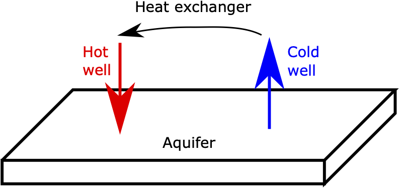
Figure 1: Schematic of the simple GeoTES simulation.
Observed geochemical composition and aquifer mineralogy
The composition of the Weber formation water has been measured at 25C and a typical analysis is shown in Table 1. Some minor points are:
Since HS is a redox species, its concentration fixes the oxidation state of the water (it is swapped with the basis species O(aq) in the simulations).
The species NH is not a basis species, but may be swapped into the basis to replace NO in the simulations.
The species B is not a basis species: B(OH) is used instead (with concentration 412mg.L).
The species Si is not a basis species: SiO(aq) is used instead (with concentration 96mg.L).
Table 1: Typical composition of the Weber formation water measured at 25C
| Species | Concentration (mg.L) |
|---|---|
| Cl- | 57400 |
| SO4– | 6030 |
| HCO3- | 3996 |
| HS- | 127 |
| Si | 45 |
| Al+++ | 3.5 |
| Ca++ | 539 |
| Mg++ | 45 |
| Fe++ | 44 |
| K+ | 1910 |
| Na+ | 36500 |
| Sr++ | 14 |
| F- | 6.1 |
| B | 72 |
| Br- | 99 |
| Ba++ | 14 |
| Li+ | 91 |
| NH3 (as N) | 33 |
| pH | 6.46 |
The mineralogy of the Weber-Tensleep aquifer has also been measured and a typical composition is shown in Table 2. The volume fractions do not sum to 100% because of small measurement errors.
Table 2: Typical mineralogy of the Weber-Tensleep aquifer
| Mineral | Volume fraction (%) |
|---|---|
| Quartz | 80.7 |
| K-feldspar | 8.0 |
| Kaolinite | 6.6E-05 |
| Siderite | 2.0 |
| Goethite | 0 |
| Pyrrhotite | 0.10 |
| Dolomite | 2.0 |
| Calcite | 5.0 |
| Fe-chlorite | 1.0 |
| Illite | 1.0 |
| Chalcedony | 0.11 |
| Anhydrite | 0.60 |
| Barite | 4.9E-05 |
| Celestite | 0 |
| Fluorite | 0 |
| Albite | 0 |
Equilibrium model at 25C
The simplest simulation possible is one that finds the molality of each primary and secondary species, given the measured concentrations of Table 1 while preventing any mineral precipitation. To perform this analysis, the concentrations shown in Table 1 must be converted to mole numbers, as shown in Table 3.
In Table 3 it is assumed that 1L of aqueous solution contains exactly 1kg of solvent water.
Table 3: Composition of the model at 25C. The pH is 6.46.
| Species | Measured conc (mg.L) | Mol weight (g/mol) | Molal (mol/kg(solvent water)) |
|---|---|---|---|
| Cl- | 57400 | 35.453 | 1.619044933 |
| SO4– | 6030 | 96.0576 | 0.062774835 |
| HCO3- | 3996 | 61.0171 | 0.065489838 |
| HS- | 127 | 33.0679 | 0.003840583 |
| SiO2(aq) | 96 | 60.0843 | 0.001597755 |
| Al+++ | 3.5 | 26.9815 | 0.000129719 |
| Ca++ | 539 | 40.08 | 0.013448104 |
| Mg++ | 45 | 24.305 | 0.001851471 |
| Fe++ | 44 | 55.847 | 0.000787867 |
| K+ | 1910 | 39.0983 | 0.048851229 |
| Na+ | 36500 | 22.9898 | 1.587660615 |
| Sr++ | 14 | 87.62 | 0.000159781 |
| F- | 6.1 | 18.9984 | 0.00032108 |
| B(OH)3 | 412 | 61.8329 | 0.006663119 |
| Br- | 99 | 79.904 | 0.001238987 |
| Ba++ | 14 | 137.33 | 0.000101944 |
| Li+ | 91 | 6.941 | 0.013110503 |
| NH3 | 33 | 17.034 | 0.001937302 |
The MOOSE model begins by defining all the basis species — those in Table 3 as well as H2O, H+ (to fix the pH) and O2(aq) (to allow for redox couples, in particular HS- and Fe+++) — as well as the minerals of interest, which are those in Table 2 with the exception of Fe-Chlorite since it is not in the database:
[UserObjects]
  [definition]
    type = GeochemicalModelDefinition
    database_file = "../../../../geochemistry/database/moose_geochemdb.json"
    basis_species = "H2O H+ Cl- SO4-- HCO3- SiO2(aq) Al+++ Ca++ Mg++ Fe++ K+ Na+ Sr++ F- B(OH)3 Br- Ba++ Li+ NO3- O2(aq)"
    equilibrium_minerals = "Siderite Pyrrhotite Dolomite Illite Anhydrite Calcite Quartz K-feldspar Kaolinite Barite Celestite Fluorite Albite Chalcedony Goethite"
  []
[]
None of the input files in this page set remove_all_extrapolated_secondary_species = true in the GeochemicalModelDefinition. Setting this flag to true removes the odd secondary species whose equilibrium constants have only been measured for a small range of temperatures, since extrapolating the experimental results can lead to unrealistic values that cause convergence issues. It is simply fortunate that the simulations on this page do not need this flag set. Generally, this flag should be set true in models involving high temperatures.
A TimeIndependentReactionSolver defines:
the swaps mentioned above (so the measured concentrations of NH3 and HS- can be used instead of NO3- and O2(aq))
the charge-balance species, which is assumed to be Cl-
the bulk mole numbers of species from Table 3 and the pH (instead of mole numbers, the geochemistry module can accept other units such as mg, if more convenient)
the temperature
that no minerals are allowed to precipitate in this exploratory simulation.
[TimeIndependentReactionSolver]
  model_definition = definition
  swap_out_of_basis = "NO3- O2(aq)"
  swap_into_basis = "  NH3  HS-"
  charge_balance_species = "Cl-"
  constraint_species = "H2O              H+       Cl-         SO4--       HCO3-       HS-         SiO2(aq)    Al+++       Ca++        Mg++        Fe++        K+          Na+         Sr++        F-         B(OH)3      Br-         Ba++        Li+         NH3"
  constraint_value = "  1.0              3.467E-7 1.619044933 0.062774835 0.065489838 0.003840583 0.001597755 0.000129719 0.013448104 0.001851471 0.000787867 0.048851229 1.587660615 0.000159781 0.00032108 0.006663119 0.001238987 0.000101944 0.013110503 0.001937302"
  constraint_meaning = "kg_solvent_water activity bulk_composition bulk_composition bulk_composition bulk_composition bulk_composition bulk_composition bulk_composition bulk_composition bulk_composition bulk_composition bulk_composition bulk_composition bulk_composition bulk_composition bulk_composition bulk_composition bulk_composition bulk_composition"
  constraint_unit = "kg dimensionless moles moles moles moles moles moles moles moles moles moles moles moles moles moles moles moles moles moles"
  prevent_precipitation = "Barite Siderite Pyrrhotite Dolomite Illite Anhydrite Calcite Quartz K-feldspar Kaolinite Celestite Fluorite Albite Chalcedony Goethite"
  ramp_max_ionic_strength_initial = 0 # not needed in this simple problem
  temperature = 25
  stoichiometric_ionic_str_using_Cl_only = true
  precision = 5
[]
The MOOSE output includes overall information:
Mass of solvent water = 1kg
Total mass = 1.103kg
Mass of aqueous solution = 1.103kg (without free minerals)
pH = 6.46
pe = -2.959
Ionic strength = 1.634mol/kg(solvent water)
Stoichiometric ionic strength = 1.704mol/kg(solvent water)
Activity of water = 0.9439
Temperature = 25
and reveals that many minerals are supersaturated, as expected because this water was sourced from an aquifer containing minerals and then cooled:
Minerals:
Illite = 5*H2O - 8*H+ + 3.5*SiO2(aq) + 2.3*Al+++ + 0.25*Mg++ + 0.6*K+;  log10K = 9.796;  SI = 9.792
Kaolinite = 5*H2O - 6*H+ + 2*SiO2(aq) + 2*Al+++;  log10K = 7.434;  SI = 7.731
K-feldspar = 2*H2O - 4*H+ + 3*SiO2(aq) + 1*Al+++ + 1*K+;  log10K = 0.06546;  SI = 7.166
Albite = 2*H2O - 4*H+ + 3*SiO2(aq) + 1*Al+++ + 1*Na+;  log10K = 3.081;  SI = 5.703
Pyrrhotite = -0.125*H2O - 0.7188*H+ + 0.03125*SO4-- + 0.875*Fe++ + 0.9688*HS-;  log10K = -5.557;  SI = 3.52
Barite = 1*SO4-- + 1*Ba++;  log10K = -9.973;  SI = 2.614
Quartz = 1*SiO2(aq);  log10K = -4.01;  SI = 1.376
Chalcedony = 1*SiO2(aq);  log10K = -3.738;  SI = 1.104
Siderite = -1*H+ + 1*HCO3- + 1*Fe++;  log10K = -0.2225;  SI = 0.8189
Dolomite = -2*H+ + 2*HCO3- + 1*Ca++ + 1*Mg++;  log10K = 2.516;  SI = 0.3859
Calcite = -1*H+ + 1*HCO3- + 1*Ca++;  log10K = 1.711;  SI = 0.01748
Fluorite = 1*Ca++ + 2*F-;  log10K = -10.97;  SI = -0.1147
Celestite = 1*SO4-- + 1*Sr++;  log10K = -6.443;  SI = -0.6262
Anhydrite = 1*SO4-- + 1*Ca++;  log10K = -4.274;  SI = -1.118
One other useful piece of information that is reported is the bulk composition of H+, which is 0.019675774mol.
Geochemical technicalities
At this point, it is worth recognising a couple of apparently strange features of the analyses presented in Table 1 and Table 2.
Barite is supersaturated. If it is allowed to precipitate then it will remove almost all of the Ba++ found in solution, seemingly contradicting Table 1. According to Table 2 Barite is found in only very small concentrations, so mechanisms must be present to prevent its precipitation, such as kinetic laws.
Both Chalcedony and Quartz are present in Table 2. Both are SiO2, but Quartz is more stable, so over time all Chalcedony should disappear. Kinetic rates may be responsible for these observations.
These complexities (and other more subtle ones) are completely ignored in the following, since the purpose of this presentation is to describe how to use the geochemistry module and not to get stuck on technical details of the geochemistry, even if they turn out to be important in real life.
A geochemical model of the Weber-Tensleep formation at 92C
The temperature of the Weber-Tensleep aquifer is approximately 92C, and its porosity is approximately 0.1. To build a geochemical model of the formation, the following process is used:
The water with composition described by Table 3 is equilibrated at 25C while preventing any precipitation of minerals (as in the previous section)
The pH constraint is removed (so no more H+ is allowed to enter the system)
The system is brought to 92C, allowing precipitation
The system is assumed to have volume 1L, or 1000cm, so is brought into contact with 9000cm of minerals with composition shown Table 2. The porosity is therefore close to (it is not exactly 0.1 due to the minor amounts of precipitation at step 4).
The resulting system is brought to equilibrium, allowing minerals to precipitate or dissolve if required, and assuming that no minerals are governed by kinetic laws
It is convenient to use the equilibrium model of the previous section to model steps 1 and 2. The bulk composition of H+ (0.019675774mol) is used, and the source mineral species are shown in Table 4. Chalcedony is not included because it dissolves in favor of Quartz, and Fe-Chlorite is not included because it does not appear in the database. To ensure the final porosity is close to 0.1,
Table 4: Mineralogy used in the model, where the porosity is assumed to be 0.1
| Mineral | Measured vol (%) | Model vol (%) | Model vol (cm) | Molar volume (cm.mol) | Moles |
|---|---|---|---|---|---|
| Siderite | 2 | 2 | 180 | 28.63 | 6.287111422 |
| Pyrrhotite | 0.1 | 0.1 | 9 | 17.62 | 0.510783201 |
| Dolomite | 2 | 2 | 180 | 64.365 | 2.796550921 |
| Illite | 1 | 1 | 90 | 138.94 | 0.647761624 |
| Chalcedony | 0.11 | 0 | 0 | 22.688 | 0 |
| Anhydrite | 0.6 | 0.6 | 54 | 45.94 | 1.175446234 |
| Calcite | 5 | 5 | 450 | 36.934 | 12.1838956 |
| Quartz | 80.7 | 81.299885 | 7316.98965 | 22.688 | 322.504833 |
| K-feldspar | 8 | 8 | 720 | 108.87 | 6.613392119 |
| Kaolinite | 6.60E-05 | 6.60E-05 | 0.00594 | 99.52 | 5.96865E-05 |
| Fe-Chlorite | 1 | 0 | 0 | 1 | 0 |
| Barite | 4.90E-05 | 4.90E-05 | 0.00441 | 52.1 | 8.46449E-05 |
| Goethite | 0 | 0 | 0 | 20.82 | 0 |
| Celestite | 0 | 0 | 0 | 46.25 | 0 |
| Fluorite | 0 | 0 | 0 | 24.54 | 0 |
| Albite | 0 | 0 | 0 | 100.07 | 0 |
The MOOSE input file uses a TimeDependentReactionSolver to raise the temperature and add the source minerals:
the first part of this input-file block is identical to the model above, save for fixing the bulk composition of H+ instead of fixing the pH
the second part adds the source minerals at rate given by Table 4 at a temperature of 95C so that the final temperature is around 92C as desired.
[TimeDependentReactionSolver]
  model_definition = definition
  geochemistry_reactor_name = reactor
  swap_out_of_basis = "NO3- O2(aq)"
  swap_into_basis = "  NH3  HS-"
  charge_balance_species = "Cl-"
  constraint_species = "H2O H+          Cl-         SO4--       HCO3-       HS-         SiO2(aq)    Al+++       Ca++        Mg++        Fe++        K+          Na+         Sr++        F-         B(OH)3      Br-         Ba++        Li+         NH3"
  constraint_value = "  1.0 0.019675774 1.619044933 0.062774835 0.065489838 0.003840583 0.001597755 0.000129719 0.013448104 0.001851471 0.000787867 0.048851229 1.587660615 0.000159781 0.00032108 0.006663119 0.001238987 0.000101944 0.013110503 0.001937302"
  constraint_meaning = "kg_solvent_water bulk_composition bulk_composition bulk_composition bulk_composition bulk_composition bulk_composition bulk_composition bulk_composition bulk_composition bulk_composition bulk_composition bulk_composition bulk_composition bulk_composition bulk_composition bulk_composition bulk_composition bulk_composition bulk_composition"
  constraint_unit = "kg moles moles moles moles moles moles moles moles moles moles moles moles moles moles moles moles moles moles moles"
  prevent_precipitation = "Celestite Fluorite Albite Chalcedony Goethite"
  ramp_max_ionic_strength_initial = 0 # not needed in this simple problem
  initial_temperature = 25
  temperature = 95 # so final temp = 92
  execute_console_output_on = 'initial timestep_end'
  source_species_names = "Siderite    Pyrrhotite  Dolomite    Illite      Anhydrite   Calcite    Quartz     K-feldspar  Kaolinite   Barite"
  source_species_rates = "6.287111422 0.510783201 2.796550921 0.647761624 1.175446234 12.1838956 322.504833 6.613392119 5.96865E-05 8.46449E-05"
  solver_info = true
  stoichiometric_ionic_str_using_Cl_only = true
[]
The MOOSE output includes the summary:
Mass of solvent water = 0.9979kg
Total mass = 25.23kg
Mass of aqueous solution = 1.096kg (without free minerals)
pH = 6.899
pe = -3.376
Ionic strength = 1.576mol/kg(solvent water)
Stoichiometric ionic strength = 1.432mol/kg(solvent water)
Activity of water = 0.9532
Temperature = 92.06
The MOOSE output also includes the composition in the species basis that consists of the minerals and free species as shown in Table 5.
Table 5: Composition of the model at 92C expressed in the basis that includes minerals and free species. The mass of solvent water is 0.99778351kg.
| Species | Bulk composition (moles) | Free |
|---|---|---|
| Quartz | 322.4086 | 322.41188 moles |
| Calcite | 12.111108 | 12.111218 moles |
| K-feldspar | 6.8269499 | 6.8276215 moles |
| Siderite | 6.2844304 | 6.2829261 moles |
| Dolomite | 2.8670301 | 2.8672731 moles |
| Anhydrite | 1.1912027 | 1.1684061 moles |
| Pyrrhotite | 0.51474767 | 0.51549555 moles |
| Illite | 0.3732507 | 0.36893829 moles |
| Kaolinite | 0.20903322 | 0.21365601 moles |
| Barite | 0.0001865889 | 0.0001853394 moles |
| Na+ | 1.5876606 | 1.4840437 molal |
| Cl- | 1.5059455 | 1.4321212 molal |
| SO4– | 0.046792579 | 0.031819079 molal |
| Li+ | 0.013110503 | 0.012928063 molal |
| B(OH)3 | 0.006663119 | 0.0014134967 molal |
| Br- | 0.001238987 | 0.0012417393 molal |
| F- | 0.00032108 | 0.00023740743 molal |
| Sr++ | 0.000159781 | 0.00013115377 molal |
| NH3 | 0.001937302 | 3.1632078e-07 molal |
It is interesting to compare the concentration of species in the model when the aqueous solution is removed from the mineral assemblage. This information is also outputted by the geochemistry module and is shown in Table 6:
The concentration of Cl- is impacted by charge-neutrality
The concentration of HCO3-, Al+++, K+ and Ba++ are all much less in the model compared with the observation due to mineral precipitation
The concentration of species not impacted by minerals is identical (Na+, Sr++, F-, B, Br-, Li+, NH3)
The model's concentration of the remaining species are similar to the observations
Table 6: Composition at 92C after removing minerals in comparison with the original measurements.
| Species | Measured conc (molal) | Model conc (molal) |
|---|---|---|
| Cl- | 1.619044933 | 1.5059455 |
| SO4– | 0.062774835 | 0.068842508 |
| HCO3- | 0.065489838 | 0.00090808324 |
| HS- | 0.003840583 | 0.0029683017 |
| SiO2(aq) | 0.001597755 | 0.00055318842 |
| Al+++ | 0.000129719 | 1.3497527e-06 |
| Ca++ | 0.013448104 | 0.022443348 |
| Mg++ | 0.001851471 | 0.00083515093 |
| Fe++ | 0.000787867 | 0.00084984977 |
| K+ | 0.048851229 | 0.0019158317 |
| Na+ | 1.587660615 | 1.5876606 |
| Sr++ | 0.000159781 | 0.000159781 |
| F- | 0.00032108 | 0.00032108 |
| B(OH)3 | 0.006663119 | 0.006663119 |
| Br- | 0.001238987 | 0.001238987 |
| Ba++ | 0.000101944 | 1.2495026e-06 |
| Li+ | 0.013110503 | 0.013110503 |
| NH3 | 0.001937302 | 0.001937302 |
The modelling also reveals that Goethite, Albite and Flourite are all supersaturated, so will probably precipitate if they are in equilibrium with the aqueous solution, apparently contradicting Table 2.
Goethite = 3.255*H2O - 0.129*Pyrrhotite - 3.345*Kaolinite + 0.8548*Calcite + 0.129*Anhydrite - 0.9839*Dolomite - 2.361*K-feldspar + 3.935*Illite + 1.113*Siderite;  log10K = -1.607;  SI = 1.539
Albite = 0.4*H2O + 0.5*SO4-- - 1.2*Kaolinite + 2*Quartz + 1*Calcite - 0.5*Anhydrite - 0.5*Dolomite - 1.2*K-feldspar + 2*Illite + 1*Na+;  log10K = -2.122;  SI = 0.8307
Fluorite = -1*SO4-- + 1*Anhydrite + 2*F-;  log10K = -5.468;  SI = 0.2909
Chalcedony = 1*Quartz;  log10K = 0.2214;  SI = -0.2214
Celestite = 1*SO4-- + 1*Sr++;  log10K = -6.861;  SI = -0.4025
The total mineral volume is reported to be 9005.244392233cm. To ensure the porosity is exactly 0.1, the free amount of Quartz is reduced by cmmol in the reactive transport simulations, leading to a bulk composition of mol.
This completes the definition of the geochemical system used in this presentation. In summary:
the bulk composition is determined by Table 5 in the basis of that table, amending Quartz to have a bulk composition of mol (the geochemistry module can use other units such as g, mg, etc, but this page uses mole-based units exclusively);
all minerals in the basis of Table 5 are assumed to be at equilibrium with the aqueous system (the
geochemistrymodule can easily handle kinetic reactions — a simple GeoTES example may be found here — but no kinetics are used in this presentation);the minerals Goethite, Albite, and Flourite are assumed to never precipitate
Scaling and heating the aqueous solution to 160C
The geochemical system just defined may be heated to 160C in order to explore potential scaling in a heat exchanger. The following method is used:
The aqueous solution is removed from the aquifer, by removing all free minerals are removed from the model just defined
The aqueous solution is slowly heated from 92C to 160C, immediately removing any precipitates as soon as they form
This technique is studying the "worst case" scenario for scaling in a heat exchanger, for it is possible that a precipitate forms only to dissolve upon further heating, but the technique used removes the precipitate and prevents its dissolution.
The TimeDependentReactionSolver defines:
the swaps needed to bring the minerals into the basis, so it is as described in Table 5;
the bulk composition of the resulting basis (from Table 5, amending Quartz to have a bulk composition of mol, recall that the geochemistry module can use other units such as grams or mg if convenient, but this page uses mole-based units exclusively);
that the Fluorite, Albite and Goethite minerals will not precipitate;
the initial temperature;
that
mode = 1is used, which means all precipitates are removed at the start of each time step;the temperature is controlled by the AuxVariable called
temp_controller.
[TimeDependentReactionSolver]
  model_definition = definition
  geochemistry_reactor_name = reactor
  swap_out_of_basis = "NO3- H+         Fe++       Ba++   SiO2(aq) Mg++     O2(aq)   Al+++   K+     Ca++      HCO3-"
  swap_into_basis = "  NH3  Pyrrhotite K-feldspar Barite Quartz   Dolomite Siderite Calcite Illite Anhydrite Kaolinite"
  charge_balance_species = "Cl-"
  constraint_species = "H2O        Quartz     Calcite   K-feldspar Siderite  Dolomite  Anhydrite Pyrrhotite Illite    Kaolinite  Barite       Na+       Cl-       SO4--       Li+         B(OH)3      Br-         F-         Sr++        NH3"
  constraint_value = "  0.99778351 322.177447 12.111108 6.8269499  6.2844304 2.8670301 1.1912027 0.51474767 0.3732507 0.20903322 0.0001865889 1.5876606 1.5059455 0.046792579 0.013110503 0.006663119 0.001238987 0.00032108 0.000159781 0.001937302"
  constraint_meaning = "kg_solvent_water bulk_composition bulk_composition bulk_composition bulk_composition bulk_composition bulk_composition bulk_composition bulk_composition bulk_composition bulk_composition bulk_composition bulk_composition bulk_composition bulk_composition bulk_composition bulk_composition bulk_composition bulk_composition bulk_composition"
  constraint_unit = "kg moles moles moles moles moles moles moles moles moles moles moles moles moles moles moles moles moles moles moles"
  prevent_precipitation = "Fluorite Albite Goethite"
  ramp_max_ionic_strength_initial = 0 # not needed in this simple problem
  initial_temperature = 92
  mode = 1 # dump all minerals at the start of each time-step
  temperature = temp_controller
  execute_console_output_on = '' # only CSV output for this problem
  stoichiometric_ionic_str_using_Cl_only = true
[]
The Executioner gives meaning to time:
[Executioner]
  type = Transient
  dt = 0.01
  end_time = 1.0
[]
The temp_controller is a simple FunctionAux:
  [temp_controller_auxk]
    type = FunctionAux
    variable = temp_controller
    function = '92 + (160 - 92) * t'
    execute_on = timestep_begin
  []
and the moles dumped to the heat exchanger (scaling) are recorded by a sequence of GeochemistryQuantityAux:
  [Anhydrite_mol_auxk]
    type = GeochemistryQuantityAux
    reactor = reactor
    variable = Anhydrite_mol
    species = Anhydrite
    quantity = moles_dumped
  []
Recording the results into Postprocessors yields the results shown in Figure 2. It is interesting to compare this with Nic Spycher's model of the Weber-Tensleep formation which predicts:
around 2kg/m(formation water) of Anhydrite, or around 0.7cm/L(formation water), which is quite similar to the current model;
around 0.03cm/L(formation water) of Dolomite, 0.01cm/L(formation water) of Calcite, 0.0025cm/L(formation water) of Siderite, while the current model predicts none of these. This could be due to a combination of a different activity model, a different geochemical model (the pH is lower), and a different definition of "scaling".
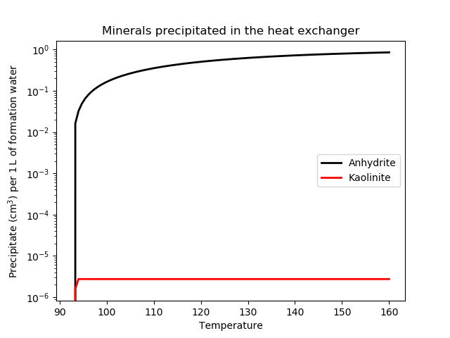
Figure 2: Degree of scaling precipitate expected in the heat exchanger according to the model of formation water.
Spatial aquifer geochemistry input file
Having created the geochemical model at 92C, it is easy to create a version that includes spatial dependence. Although the input file may be run by itself, no interesting phenomena will be observed since the temperature will be fiexed and source-species rates will be zero. When coupled with a porous_flow input file (described below) the temperature and source-species rates will be non-trivial. The input file begins with a GeochemicalModelDefinition:
[UserObjects]
  [definition]
    type = GeochemicalModelDefinition
    database_file = '../../../../geochemistry/database/moose_geochemdb.json'
    basis_species = 'H2O H+ Cl- SO4-- HCO3- SiO2(aq) Al+++ Ca++ Mg++ Fe++ K+ Na+ Sr++ F- B(OH)3 Br- Ba++ Li+ NO3- O2(aq)'
    equilibrium_minerals = 'Siderite Pyrrhotite Dolomite Illite Anhydrite Calcite Quartz K-feldspar Kaolinite Barite Celestite Fluorite Albite Chalcedony Goethite'
  []
  [nodal_void_volume_uo]
    type = NodalVoidVolume
    porosity = porosity
    execute_on = 'initial timestep_end' # initial means this is evaluated properly for the first timestep
  []
[]
The SpatialReactionSolver defines:
the swaps needed to bring the basis to the state defined in Table 5
the initial composition of Table 5 (amending Quartz to have a bulk composition of mol). Please note the key concept that each finite element node considers just 1 litre of aqueous solution
the
initial_temperaturethat the temperature at each finite-element node will be controlled by the
temperatureAuxVariable (which will be provided by the parentporous_flowsimulation)the source species, and their rates per 1 litre of aqueous solution
that various AuxVariables are not needed in this simulation
[SpatialReactionSolver]
  model_definition = definition
  geochemistry_reactor_name = reactor
  charge_balance_species = 'Cl-'
  swap_out_of_basis = 'NO3- H+         Fe++       Ba++   SiO2(aq) Mg++     O2(aq)   Al+++   K+     Ca++      HCO3-'
  swap_into_basis = '  NH3  Pyrrhotite K-feldspar Barite Quartz   Dolomite Siderite Calcite Illite Anhydrite Kaolinite'
  # ASSUME that 1 litre of solution contains:
  constraint_species = 'H2O        Quartz     Calcite   K-feldspar Siderite  Dolomite  Anhydrite Pyrrhotite Illite    Kaolinite  Barite       Na+       Cl-       SO4--       Li+         B(OH)3      Br-         F-         Sr++        NH3'
  constraint_value = '  0.99778351 322.177447 12.111108 6.8269499  6.2844304 2.8670301 1.1912027 0.51474767 0.3732507 0.20903322 0.0001865889 1.5876606 1.5059455 0.046792579 0.013110503 0.006663119 0.001238987 0.00032108 0.000159781 0.001937302'
  constraint_meaning = 'kg_solvent_water bulk_composition bulk_composition bulk_composition bulk_composition bulk_composition bulk_composition bulk_composition bulk_composition bulk_composition bulk_composition bulk_composition bulk_composition bulk_composition bulk_composition bulk_composition bulk_composition bulk_composition bulk_composition bulk_composition'
  constraint_unit = "kg moles moles moles moles moles moles moles moles moles moles moles moles moles moles moles moles moles moles moles"
  prevent_precipitation = 'Fluorite Albite Goethite'
  initial_temperature = 92
  temperature = temperature
  source_species_names = 'H+ Cl- SO4-- HCO3- SiO2(aq) Al+++ Ca++ Mg++ Fe++ K+ Na+ Sr++ F- B(OH)3 Br- Ba++ Li+ NO3- O2(aq) H2O'
  source_species_rates = ' rate_H_per_1l rate_Cl_per_1l rate_SO4_per_1l rate_HCO3_per_1l rate_SiO2aq_per_1l rate_Al_per_1l rate_Ca_per_1l rate_Mg_per_1l rate_Fe_per_1l rate_K_per_1l rate_Na_per_1l rate_Sr_per_1l rate_F_per_1l rate_BOH_per_1l rate_Br_per_1l rate_Ba_per_1l rate_Li_per_1l rate_NO3_per_1l rate_O2aq_per_1l rate_H2O_per_1l'
  ramp_max_ionic_strength_initial = 0 # max_ionic_strength in such a simple problem does not need ramping
  execute_console_output_on = '' # only CSV and exodus output for this simulation
  add_aux_molal = false # save some memory and reduce variables in output exodus
  add_aux_mg_per_kg = false # save some memory and reduce variables in output exodus
  add_aux_free_mg = false # save some memory and reduce variables in output exodus
  add_aux_activity = false # save some memory and reduce variables in output exodus
  add_aux_bulk_moles = false # save some memory and reduce variables in output exodus
  adaptive_timestepping = true
[]
The remainder of the input file is mostly concerned with translating between porous-flow information (mass fractions and source rates at each node) and geochemistry information (moles in each litre of fluid). This block translates the porous_flow rate, which is the rate of change of a species mass at each node (in kg.s) into a rate of change per 1 litre of aqueous solution at each node:
  [rate_H_per_1l_auxk]
    type = ParsedAux
    args = 'pf_rate_H nodal_void_volume'
    variable = rate_H_per_1l
    function = 'pf_rate_H / 1.0079 / nodal_void_volume'
    execute_on = 'timestep_end'
  []
Here 1.0079 is the molar mass (g.mol) of the species H, and nodal_void_volume is the volume of aqueous solution held at each node. This block translates the geochemistry moles of transported H into a mass fraction of H:
  [massfrac_H_auxk]
    type = ParsedAux
    args = 'transported_H transported_mass'
    variable = massfrac_H
    function = 'transported_H * 1.0079 / transported_mass'
    execute_on = 'timestep_end'
  []
using the transported_mass, which is
  [transported_mass_auxk]
    type = ParsedAux
    args = ' transported_H transported_Cl transported_SO4 transported_HCO3 transported_SiO2aq transported_Al transported_Ca transported_Mg transported_Fe transported_K transported_Na transported_Sr transported_F transported_BOH transported_Br transported_Ba transported_Li transported_NO3 transported_O2aq transported_H2O'
    variable = transported_mass
    function = 'transported_H * 1.0079 + transported_Cl * 35.453 + transported_SO4 * 96.0576 + transported_HCO3 * 61.0171 + transported_SiO2aq * 60.0843 + transported_Al * 26.9815 + transported_Ca * 40.08 + transported_Mg * 24.305 + transported_Fe * 55.847 + transported_K * 39.0983 + transported_Na * 22.9898 + transported_Sr * 87.62 + transported_F * 18.9984 + transported_BOH * 61.8329 + transported_Br * 79.904 + transported_Ba * 137.33 + transported_Li * 6.941 + transported_NO3 * 62.0049 + transported_O2aq * 31.9988 + transported_H2O * 18.01801802'
    execute_on = 'timestep_end'
  []
The porosity is calculated using the free mineral volumes:
  [porosity_auxk]
    type = ParsedAux
    args = 'free_cm3_Siderite free_cm3_Pyrrhotite free_cm3_Dolomite free_cm3_Illite free_cm3_Anhydrite free_cm3_Calcite free_cm3_Quartz free_cm3_Kfeldspar free_cm3_Kaolinite free_cm3_Barite free_cm3_Celestite free_cm3_Fluorite free_cm3_Albite free_cm3_Chalcedony free_cm3_Goethite'
    function = '1000.0 / (1000.0 + free_cm3_Siderite + free_cm3_Pyrrhotite + free_cm3_Dolomite + free_cm3_Illite + free_cm3_Anhydrite + free_cm3_Calcite + free_cm3_Quartz + free_cm3_Kfeldspar + free_cm3_Kaolinite + free_cm3_Barite + free_cm3_Celestite + free_cm3_Fluorite + free_cm3_Albite + free_cm3_Chalcedony + free_cm3_Goethite)'
    variable = porosity
    execute_on = 'timestep_end'
  []
Injection, production and porous flow
The Weber-Tensleep aquifer is around 200m thick, and injecting and producing over its entire thickness may lead to unacceptably low efficiencies as the buoyant hot water rises to the top of the aquifer, never to be recovered. For the purposes of this example, assume there is a 10m thick horizontal aquifer, bounded above and below by caps. The physical properties are listed in Table 7.
Table 7: Physical properties of the aquifer and caps
| Property | Quantity |
|---|---|
| Aquifer thickness | 10m |
| Aquifer depth | 3000m |
| Aquifer initial porepressure | 30MPa |
| Aquifer initial temperature | 92C |
| Aquifer horizontal permeability | m |
| Aquifer vertical permeability | m |
| Aquifer porosity | 0.1 |
| Aquifer thermal conductivity | 1.3W.m.K |
| Cap thickness | 20m |
| Cap isotropic permeability | m |
| Cap porosity | 0.01 |
| Cap thermal conductivity | 1.3W.m.K |
| Geothermal gradient | 0 |
As shown in Figure 1, the well geometry consists of a single vertical well injecting over the entire aquifer thickness and a single vertical well producing over the entire aquifer thickness. Only the injection phase of the GeoTES system is explored here, with parameters listed in Table 8. The injection and production rates are chosen so that the porepressure remains positive at the production well given the relatively low aquifer permeability.
Table 8: Injection parameters of the GeoTES system
| Property | Quantity |
|---|---|
| Injection and production rate | 0.2kg.s |
| Injection temperature | 160C |
| Injection fluid | Heated production water: all precipitates removed |
| Injection time | 90days |
| Distance between wells | 50m |
The injection-production simulation may be performed using the porous_flow module. Because this presentation is focussing on geochemistry, only the highlights of the porous_flow input file are mentioned.
The variables are the mass-fractions of each transported species (which are those in the original geochemical basis before any swaps), called f_H, f_Cl, f_SO4, etc, with initial condition defined by Table 6 and converted into mass-fractions as shown in Table 9.
Table 9: Composition at 92C of transported species (ie, not including minerals) expressed in the original basis.
| Species | Moles | Molar weight (g.mol) | Mass (g) | Mass fraction |
|---|---|---|---|---|
| H2O | 55.38 | 18.01801802 | 997.8378378 | 0.910314278 |
| H+ | -0.003232 | 1.0079 | -0.003257533 | -2.9718E-06 |
| Cl- | 1.506 | 35.453 | 53.392218 | 0.048709015 |
| SO4– | 0.06887 | 96.0576 | 6.615486912 | 0.006035221 |
| HCO3- | 0.0009061 | 61.0171 | 0.055287594 | 5.04381E-05 |
| SiO2(aq) | 0.0005525 | 60.0843 | 0.033196576 | 3.02848E-05 |
| Al+++ | 1.35E-06 | 26.9815 | 3.6479E-05 | 3.32793E-08 |
| Ca++ | 0.02247 | 40.08 | 0.9005976 | 0.000821603 |
| Mg++ | 0.0008366 | 24.305 | 0.020333563 | 1.855E-05 |
| Fe++ | 0.0008498 | 55.847 | 0.047458781 | 4.3296E-05 |
| K+ | 0.001913 | 39.0983 | 0.074795048 | 6.82345E-05 |
| Na+ | 1.588 | 22.9898 | 36.5078024 | 0.033305586 |
| Sr++ | 0.0001598 | 87.62 | 0.014001676 | 1.27735E-05 |
| F- | 0.0003211 | 18.9984 | 0.006100386 | 5.5653E-06 |
| B(OH)3 | 0.006663 | 61.8329 | 0.411992613 | 0.000375855 |
| Br- | 0.001239 | 79.904 | 0.099001056 | 9.03174E-05 |
| Ba++ | 1.25E-06 | 137.33 | 0.000171388 | 1.56355E-07 |
| Li+ | 0.01311 | 6.941 | 0.09099651 | 8.30149E-05 |
| NO3- | 0.001937 | 62.0049 | 0.120103491 | 0.000109569 |
| O2(aq) | -0.002426 | 31.9988 | -0.077629089 | -7.082E-05 |
To interface with the child geochemistry simulation (detailed above), the rates of change of each transported species must be recorded. This is performed via the save_component_rate_in feature of the PorousFlowFullySaturated Action:
#########################################
#                                       #
# File written by create_input_files.py #
#                                       #
#########################################
# PorousFlow simulation of injection and production in a simplified GeoTES aquifer
# Much of this file is standard porous-flow stuff.  The unusual aspects are:
# - transfer of the rates of changes of each species (kg.s) to the aquifer_geochemistry.i simulation.  This is achieved by saving these changes from the PorousFlowMassTimeDerivative residuals
# - transfer of the temperature field to the aquifer_geochemistry.i simulation
# Interesting behaviour can be simulated by this file without its 'parent' simulation, exchanger.i.  exchanger.i provides mass-fractions injected via the injection_rate_massfrac_* variables, but since these are more-or-less constant throughout the duration of the exchanger.i simulation, the initial_conditions specified below may be used.  Similar, exchanger.i provides injection_temperature, but that is also constant.
injection_rate = -0.02 # kg/s/m, negative because injection as a source
production_rate = 0.02 # kg/s/m, this is about the maximum that can be sustained by the aquifer, with its fairly low permeability, without porepressure becoming negative
[Mesh]
  [gen]
    type = GeneratedMeshGenerator
    dim = 3
    xmin = -75
    xmax = 75
    ymin = 0
    ymax = 40
    zmin = -25
    zmax = 25
    nx = 15
    ny = 4
    nz = 5
  []
  [aquifer]
    type = ParsedSubdomainMeshGenerator
    input = gen
    block_id = 1
    block_name = aquifer
    combinatorial_geometry = 'z >= -5 & z <= 5'
  []
  [injection_nodes]
    input = aquifer
    type = ExtraNodesetGenerator
    new_boundary = injection_nodes
    coord = '-25 0 -5; -25 0 5'
  []
  [production_nodes]
    input = injection_nodes
    type = ExtraNodesetGenerator
    new_boundary = production_nodes
    coord = '25 0 -5; 25 0 5'
  []
[]

[GlobalParams]
  PorousFlowDictator = dictator
  gravity = '0 0 -10'
[]

[BCs]
  [injection_temperature]
    type = MatchedValueBC
    variable = temperature
    v = injection_temperature
    boundary = injection_nodes
  []
[]

[Modules]
  [FluidProperties]
    [the_simple_fluid]
      type = SimpleFluidProperties
      thermal_expansion = 0
      bulk_modulus = 2E9
      viscosity = 1E-3
      density0 = 1000
      cv = 4000.0
      cp = 4000.0
    []
  []
[]

[PorousFlowFullySaturated]
  coupling_type = ThermoHydro
  porepressure = porepressure
  temperature = temperature
  mass_fraction_vars = 'f_H f_Cl f_SO4 f_HCO3 f_SiO2aq f_Al f_Ca f_Mg f_Fe f_K f_Na f_Sr f_F f_BOH f_Br f_Ba f_Li f_NO3 f_O2aq '
  save_component_rate_in = 'rate_H rate_Cl rate_SO4 rate_HCO3 rate_SiO2aq rate_Al rate_Ca rate_Mg rate_Fe rate_K rate_Na rate_Sr rate_F rate_BOH rate_Br rate_Ba rate_Li rate_NO3 rate_O2aq rate_H2O' # change in kg at every node / dt
  fp = the_simple_fluid
  temperature_unit = Celsius
[]

[Materials]
  [porosity_caps]
    type = PorousFlowPorosityConst # this simulation has no porosity changes from dissolution
    block = 0
    porosity = 0.01
  []
  [porosity_aquifer]
    type = PorousFlowPorosityConst # this simulation has no porosity changes from dissolution
    block = aquifer
    porosity = 0.063
  []
  [permeability_caps]
    type = PorousFlowPermeabilityConst
    block = 0
    permeability = '1E-18 0 0   0 1E-18 0   0 0 1E-18'
  []
  [permeability_aquifer]
    type = PorousFlowPermeabilityConst
    block = aquifer
    permeability = '1.7E-15 0 0   0 1.7E-15 0   0 0 4.1E-16'
  []
  [thermal_conductivity]
    type = PorousFlowThermalConductivityIdeal
    dry_thermal_conductivity = '0 0 0  0 0 0  0 0 0'
  []
  [rock_heat]
    type = PorousFlowMatrixInternalEnergy
    density = 2500.0
    specific_heat_capacity = 1200.0
  []
[]

[Preconditioning]
  active = typically_efficient
  [typically_efficient]
    type = SMP
    full = true
    petsc_options_iname = '-pc_type -pc_hypre_type'
    petsc_options_value = ' hypre    boomeramg'
  []
  [strong]
    type = SMP
    full = true
    petsc_options = '-ksp_diagonal_scale -ksp_diagonal_scale_fix'
    petsc_options_iname = '-pc_type -sub_pc_type -sub_pc_factor_shift_type -pc_asm_overlap'
    petsc_options_value = ' asm      ilu           NONZERO                   2'
  []
  [probably_too_strong]
    type = SMP
    full = true
    petsc_options_iname = '-pc_type -pc_factor_mat_solver_package'
    petsc_options_value = ' lu       mumps'
  []
[]

[Executioner]
  type = Transient
  solve_type = Newton
  end_time = 7.76E6 # 90 days
  [TimeStepper]
    type = FunctionDT
    function = 'min(3E4, max(1E4, 0.2 * t))'
  []
[]

[Outputs]
  exodus = true
[]

[Variables]
  [f_H]
    initial_condition = -2.952985071156e-06
  []
  [f_Cl]
    initial_condition = 0.04870664551708
  []
  [f_SO4]
    initial_condition = 0.0060359986852517
  []
  [f_HCO3]
    initial_condition = 5.0897287594019e-05
  []
  [f_SiO2aq]
    initial_condition = 3.0246609868421e-05
  []
  [f_Al]
    initial_condition = 3.268028901929e-08
  []
  [f_Ca]
    initial_condition = 0.00082159428184586
  []
  [f_Mg]
    initial_condition = 1.8546347062146e-05
  []
  [f_Fe]
    initial_condition = 4.3291908204093e-05
  []
  [f_K]
    initial_condition = 6.8434768308898e-05
  []
  [f_Na]
    initial_condition = 0.033298053919671
  []
  [f_Sr]
    initial_condition = 1.2771866652177e-05
  []
  [f_F]
    initial_condition = 5.5648860174073e-06
  []
  [f_BOH]
    initial_condition = 0.0003758574621917
  []
  [f_Br]
    initial_condition = 9.0315286107068e-05
  []
  [f_Ba]
    initial_condition = 1.5637460875161e-07
  []
  [f_Li]
    initial_condition = 8.3017067912701e-05
  []
  [f_NO3]
    initial_condition = 0.00010958455036169
  []
  [f_O2aq]
    initial_condition = -7.0806852373351e-05
  []
  [porepressure]
    initial_condition = 30E6
  []
  [temperature]
    initial_condition = 92
    scaling = 1E-6 # fluid enthalpy is roughly 1E6
  []
[]

[DiracKernels]
  [inject_H]
    type = PorousFlowPolyLineSink
    SumQuantityUO = injected_mass
    fluxes = ${injection_rate}
    p_or_t_vals = 0.0
    multiplying_var = injection_rate_massfrac_H
    point_file = injection.bh
    variable = f_H
  []
  [inject_Cl]
    type = PorousFlowPolyLineSink
    SumQuantityUO = injected_mass
    fluxes = ${injection_rate}
    p_or_t_vals = 0.0
    multiplying_var = injection_rate_massfrac_Cl
    point_file = injection.bh
    variable = f_Cl
  []
  [inject_SO4]
    type = PorousFlowPolyLineSink
    SumQuantityUO = injected_mass
    fluxes = ${injection_rate}
    p_or_t_vals = 0.0
    multiplying_var = injection_rate_massfrac_SO4
    point_file = injection.bh
    variable = f_SO4
  []
  [inject_HCO3]
    type = PorousFlowPolyLineSink
    SumQuantityUO = injected_mass
    fluxes = ${injection_rate}
    p_or_t_vals = 0.0
    multiplying_var = injection_rate_massfrac_HCO3
    point_file = injection.bh
    variable = f_HCO3
  []
  [inject_SiO2aq]
    type = PorousFlowPolyLineSink
    SumQuantityUO = injected_mass
    fluxes = ${injection_rate}
    p_or_t_vals = 0.0
    multiplying_var = injection_rate_massfrac_SiO2aq
    point_file = injection.bh
    variable = f_SiO2aq
  []
  [inject_Al]
    type = PorousFlowPolyLineSink
    SumQuantityUO = injected_mass
    fluxes = ${injection_rate}
    p_or_t_vals = 0.0
    multiplying_var = injection_rate_massfrac_Al
    point_file = injection.bh
    variable = f_Al
  []
  [inject_Ca]
    type = PorousFlowPolyLineSink
    SumQuantityUO = injected_mass
    fluxes = ${injection_rate}
    p_or_t_vals = 0.0
    multiplying_var = injection_rate_massfrac_Ca
    point_file = injection.bh
    variable = f_Ca
  []
  [inject_Mg]
    type = PorousFlowPolyLineSink
    SumQuantityUO = injected_mass
    fluxes = ${injection_rate}
    p_or_t_vals = 0.0
    multiplying_var = injection_rate_massfrac_Mg
    point_file = injection.bh
    variable = f_Mg
  []
  [inject_Fe]
    type = PorousFlowPolyLineSink
    SumQuantityUO = injected_mass
    fluxes = ${injection_rate}
    p_or_t_vals = 0.0
    multiplying_var = injection_rate_massfrac_Fe
    point_file = injection.bh
    variable = f_Fe
  []
  [inject_K]
    type = PorousFlowPolyLineSink
    SumQuantityUO = injected_mass
    fluxes = ${injection_rate}
    p_or_t_vals = 0.0
    multiplying_var = injection_rate_massfrac_K
    point_file = injection.bh
    variable = f_K
  []
  [inject_Na]
    type = PorousFlowPolyLineSink
    SumQuantityUO = injected_mass
    fluxes = ${injection_rate}
    p_or_t_vals = 0.0
    multiplying_var = injection_rate_massfrac_Na
    point_file = injection.bh
    variable = f_Na
  []
  [inject_Sr]
    type = PorousFlowPolyLineSink
    SumQuantityUO = injected_mass
    fluxes = ${injection_rate}
    p_or_t_vals = 0.0
    multiplying_var = injection_rate_massfrac_Sr
    point_file = injection.bh
    variable = f_Sr
  []
  [inject_F]
    type = PorousFlowPolyLineSink
    SumQuantityUO = injected_mass
    fluxes = ${injection_rate}
    p_or_t_vals = 0.0
    multiplying_var = injection_rate_massfrac_F
    point_file = injection.bh
    variable = f_F
  []
  [inject_BOH]
    type = PorousFlowPolyLineSink
    SumQuantityUO = injected_mass
    fluxes = ${injection_rate}
    p_or_t_vals = 0.0
    multiplying_var = injection_rate_massfrac_BOH
    point_file = injection.bh
    variable = f_BOH
  []
  [inject_Br]
    type = PorousFlowPolyLineSink
    SumQuantityUO = injected_mass
    fluxes = ${injection_rate}
    p_or_t_vals = 0.0
    multiplying_var = injection_rate_massfrac_Br
    point_file = injection.bh
    variable = f_Br
  []
  [inject_Ba]
    type = PorousFlowPolyLineSink
    SumQuantityUO = injected_mass
    fluxes = ${injection_rate}
    p_or_t_vals = 0.0
    multiplying_var = injection_rate_massfrac_Ba
    point_file = injection.bh
    variable = f_Ba
  []
  [inject_Li]
    type = PorousFlowPolyLineSink
    SumQuantityUO = injected_mass
    fluxes = ${injection_rate}
    p_or_t_vals = 0.0
    multiplying_var = injection_rate_massfrac_Li
    point_file = injection.bh
    variable = f_Li
  []
  [inject_NO3]
    type = PorousFlowPolyLineSink
    SumQuantityUO = injected_mass
    fluxes = ${injection_rate}
    p_or_t_vals = 0.0
    multiplying_var = injection_rate_massfrac_NO3
    point_file = injection.bh
    variable = f_NO3
  []
  [inject_O2aq]
    type = PorousFlowPolyLineSink
    SumQuantityUO = injected_mass
    fluxes = ${injection_rate}
    p_or_t_vals = 0.0
    multiplying_var = injection_rate_massfrac_O2aq
    point_file = injection.bh
    variable = f_O2aq
  []
  [inject_H2O]
    type = PorousFlowPolyLineSink
    SumQuantityUO = injected_mass
    fluxes = ${injection_rate}
    p_or_t_vals = 0.0
    multiplying_var = injection_rate_massfrac_H2O
    point_file = injection.bh
    variable = porepressure
  []

  [produce_H]
    type = PorousFlowPolyLineSink
    SumQuantityUO = produced_mass_H
    fluxes = ${production_rate}
    p_or_t_vals = 0.0
    mass_fraction_component = 0
    point_file = production.bh
    variable = f_H
  []
  [produce_Cl]
    type = PorousFlowPolyLineSink
    SumQuantityUO = produced_mass_Cl
    fluxes = ${production_rate}
    p_or_t_vals = 0.0
    mass_fraction_component = 1
    point_file = production.bh
    variable = f_Cl
  []
  [produce_SO4]
    type = PorousFlowPolyLineSink
    SumQuantityUO = produced_mass_SO4
    fluxes = ${production_rate}
    p_or_t_vals = 0.0
    mass_fraction_component = 2
    point_file = production.bh
    variable = f_SO4
  []
  [produce_HCO3]
    type = PorousFlowPolyLineSink
    SumQuantityUO = produced_mass_HCO3
    fluxes = ${production_rate}
    p_or_t_vals = 0.0
    mass_fraction_component = 3
    point_file = production.bh
    variable = f_HCO3
  []
  [produce_SiO2aq]
    type = PorousFlowPolyLineSink
    SumQuantityUO = produced_mass_SiO2aq
    fluxes = ${production_rate}
    p_or_t_vals = 0.0
    mass_fraction_component = 4
    point_file = production.bh
    variable = f_SiO2aq
  []
  [produce_Al]
    type = PorousFlowPolyLineSink
    SumQuantityUO = produced_mass_Al
    fluxes = ${production_rate}
    p_or_t_vals = 0.0
    mass_fraction_component = 5
    point_file = production.bh
    variable = f_Al
  []
  [produce_Ca]
    type = PorousFlowPolyLineSink
    SumQuantityUO = produced_mass_Ca
    fluxes = ${production_rate}
    p_or_t_vals = 0.0
    mass_fraction_component = 6
    point_file = production.bh
    variable = f_Ca
  []
  [produce_Mg]
    type = PorousFlowPolyLineSink
    SumQuantityUO = produced_mass_Mg
    fluxes = ${production_rate}
    p_or_t_vals = 0.0
    mass_fraction_component = 7
    point_file = production.bh
    variable = f_Mg
  []
  [produce_Fe]
    type = PorousFlowPolyLineSink
    SumQuantityUO = produced_mass_Fe
    fluxes = ${production_rate}
    p_or_t_vals = 0.0
    mass_fraction_component = 8
    point_file = production.bh
    variable = f_Fe
  []
  [produce_K]
    type = PorousFlowPolyLineSink
    SumQuantityUO = produced_mass_K
    fluxes = ${production_rate}
    p_or_t_vals = 0.0
    mass_fraction_component = 9
    point_file = production.bh
    variable = f_K
  []
  [produce_Na]
    type = PorousFlowPolyLineSink
    SumQuantityUO = produced_mass_Na
    fluxes = ${production_rate}
    p_or_t_vals = 0.0
    mass_fraction_component = 10
    point_file = production.bh
    variable = f_Na
  []
  [produce_Sr]
    type = PorousFlowPolyLineSink
    SumQuantityUO = produced_mass_Sr
    fluxes = ${production_rate}
    p_or_t_vals = 0.0
    mass_fraction_component = 11
    point_file = production.bh
    variable = f_Sr
  []
  [produce_F]
    type = PorousFlowPolyLineSink
    SumQuantityUO = produced_mass_F
    fluxes = ${production_rate}
    p_or_t_vals = 0.0
    mass_fraction_component = 12
    point_file = production.bh
    variable = f_F
  []
  [produce_BOH]
    type = PorousFlowPolyLineSink
    SumQuantityUO = produced_mass_BOH
    fluxes = ${production_rate}
    p_or_t_vals = 0.0
    mass_fraction_component = 13
    point_file = production.bh
    variable = f_BOH
  []
  [produce_Br]
    type = PorousFlowPolyLineSink
    SumQuantityUO = produced_mass_Br
    fluxes = ${production_rate}
    p_or_t_vals = 0.0
    mass_fraction_component = 14
    point_file = production.bh
    variable = f_Br
  []
  [produce_Ba]
    type = PorousFlowPolyLineSink
    SumQuantityUO = produced_mass_Ba
    fluxes = ${production_rate}
    p_or_t_vals = 0.0
    mass_fraction_component = 15
    point_file = production.bh
    variable = f_Ba
  []
  [produce_Li]
    type = PorousFlowPolyLineSink
    SumQuantityUO = produced_mass_Li
    fluxes = ${production_rate}
    p_or_t_vals = 0.0
    mass_fraction_component = 16
    point_file = production.bh
    variable = f_Li
  []
  [produce_NO3]
    type = PorousFlowPolyLineSink
    SumQuantityUO = produced_mass_NO3
    fluxes = ${production_rate}
    p_or_t_vals = 0.0
    mass_fraction_component = 17
    point_file = production.bh
    variable = f_NO3
  []
  [produce_O2aq]
    type = PorousFlowPolyLineSink
    SumQuantityUO = produced_mass_O2aq
    fluxes = ${production_rate}
    p_or_t_vals = 0.0
    mass_fraction_component = 18
    point_file = production.bh
    variable = f_O2aq
  []
  [produce_H2O]
    type = PorousFlowPolyLineSink
    SumQuantityUO = produced_mass_H2O
    fluxes = ${production_rate}
    p_or_t_vals = 0.0
    mass_fraction_component = 19
    point_file = production.bh
    variable = porepressure
  []
  [produce_heat]
    type = PorousFlowPolyLineSink
    SumQuantityUO = produced_heat
    fluxes = ${production_rate}
    p_or_t_vals = 0.0
    use_enthalpy = true
    point_file = production.bh
    variable = temperature
  []
[]

[UserObjects]
  [injected_mass]
    type = PorousFlowSumQuantity
  []
  [produced_mass_H]
    type = PorousFlowSumQuantity
  []
  [produced_mass_Cl]
    type = PorousFlowSumQuantity
  []
  [produced_mass_SO4]
    type = PorousFlowSumQuantity
  []
  [produced_mass_HCO3]
    type = PorousFlowSumQuantity
  []
  [produced_mass_SiO2aq]
    type = PorousFlowSumQuantity
  []
  [produced_mass_Al]
    type = PorousFlowSumQuantity
  []
  [produced_mass_Ca]
    type = PorousFlowSumQuantity
  []
  [produced_mass_Mg]
    type = PorousFlowSumQuantity
  []
  [produced_mass_Fe]
    type = PorousFlowSumQuantity
  []
  [produced_mass_K]
    type = PorousFlowSumQuantity
  []
  [produced_mass_Na]
    type = PorousFlowSumQuantity
  []
  [produced_mass_Sr]
    type = PorousFlowSumQuantity
  []
  [produced_mass_F]
    type = PorousFlowSumQuantity
  []
  [produced_mass_BOH]
    type = PorousFlowSumQuantity
  []
  [produced_mass_Br]
    type = PorousFlowSumQuantity
  []
  [produced_mass_Ba]
    type = PorousFlowSumQuantity
  []
  [produced_mass_Li]
    type = PorousFlowSumQuantity
  []
  [produced_mass_NO3]
    type = PorousFlowSumQuantity
  []
  [produced_mass_O2aq]
    type = PorousFlowSumQuantity
  []
  [produced_mass_H2O]
    type = PorousFlowSumQuantity
  []
  [produced_heat]
    type = PorousFlowSumQuantity
  []
[]

[Postprocessors]
  [dt]
    type = TimestepSize
    execute_on = TIMESTEP_BEGIN
  []
  [tot_kg_injected_this_timestep]
    type = PorousFlowPlotQuantity
    uo = injected_mass
  []
  [kg_H_produced_this_timestep]
    type = PorousFlowPlotQuantity
    uo = produced_mass_H
  []
  [kg_Cl_produced_this_timestep]
    type = PorousFlowPlotQuantity
    uo = produced_mass_Cl
  []
  [kg_SO4_produced_this_timestep]
    type = PorousFlowPlotQuantity
    uo = produced_mass_SO4
  []
  [kg_HCO3_produced_this_timestep]
    type = PorousFlowPlotQuantity
    uo = produced_mass_HCO3
  []
  [kg_SiO2aq_produced_this_timestep]
    type = PorousFlowPlotQuantity
    uo = produced_mass_SiO2aq
  []
  [kg_Al_produced_this_timestep]
    type = PorousFlowPlotQuantity
    uo = produced_mass_Al
  []
  [kg_Ca_produced_this_timestep]
    type = PorousFlowPlotQuantity
    uo = produced_mass_Ca
  []
  [kg_Mg_produced_this_timestep]
    type = PorousFlowPlotQuantity
    uo = produced_mass_Mg
  []
  [kg_Fe_produced_this_timestep]
    type = PorousFlowPlotQuantity
    uo = produced_mass_Fe
  []
  [kg_K_produced_this_timestep]
    type = PorousFlowPlotQuantity
    uo = produced_mass_K
  []
  [kg_Na_produced_this_timestep]
    type = PorousFlowPlotQuantity
    uo = produced_mass_Na
  []
  [kg_Sr_produced_this_timestep]
    type = PorousFlowPlotQuantity
    uo = produced_mass_Sr
  []
  [kg_F_produced_this_timestep]
    type = PorousFlowPlotQuantity
    uo = produced_mass_F
  []
  [kg_BOH_produced_this_timestep]
    type = PorousFlowPlotQuantity
    uo = produced_mass_BOH
  []
  [kg_Br_produced_this_timestep]
    type = PorousFlowPlotQuantity
    uo = produced_mass_Br
  []
  [kg_Ba_produced_this_timestep]
    type = PorousFlowPlotQuantity
    uo = produced_mass_Ba
  []
  [kg_Li_produced_this_timestep]
    type = PorousFlowPlotQuantity
    uo = produced_mass_Li
  []
  [kg_NO3_produced_this_timestep]
    type = PorousFlowPlotQuantity
    uo = produced_mass_NO3
  []
  [kg_O2aq_produced_this_timestep]
    type = PorousFlowPlotQuantity
    uo = produced_mass_O2aq
  []
  [kg_H2O_produced_this_timestep]
    type = PorousFlowPlotQuantity
    uo = produced_mass_H2O
  []
  [mole_rate_H_produced]
    type = FunctionValuePostprocessor
    function = moles_H
  []
  [mole_rate_Cl_produced]
    type = FunctionValuePostprocessor
    function = moles_Cl
  []
  [mole_rate_SO4_produced]
    type = FunctionValuePostprocessor
    function = moles_SO4
  []
  [mole_rate_HCO3_produced]
    type = FunctionValuePostprocessor
    function = moles_HCO3
  []
  [mole_rate_SiO2aq_produced]
    type = FunctionValuePostprocessor
    function = moles_SiO2aq
  []
  [mole_rate_Al_produced]
    type = FunctionValuePostprocessor
    function = moles_Al
  []
  [mole_rate_Ca_produced]
    type = FunctionValuePostprocessor
    function = moles_Ca
  []
  [mole_rate_Mg_produced]
    type = FunctionValuePostprocessor
    function = moles_Mg
  []
  [mole_rate_Fe_produced]
    type = FunctionValuePostprocessor
    function = moles_Fe
  []
  [mole_rate_K_produced]
    type = FunctionValuePostprocessor
    function = moles_K
  []
  [mole_rate_Na_produced]
    type = FunctionValuePostprocessor
    function = moles_Na
  []
  [mole_rate_Sr_produced]
    type = FunctionValuePostprocessor
    function = moles_Sr
  []
  [mole_rate_F_produced]
    type = FunctionValuePostprocessor
    function = moles_F
  []
  [mole_rate_BOH_produced]
    type = FunctionValuePostprocessor
    function = moles_BOH
  []
  [mole_rate_Br_produced]
    type = FunctionValuePostprocessor
    function = moles_Br
  []
  [mole_rate_Ba_produced]
    type = FunctionValuePostprocessor
    function = moles_Ba
  []
  [mole_rate_Li_produced]
    type = FunctionValuePostprocessor
    function = moles_Li
  []
  [mole_rate_NO3_produced]
    type = FunctionValuePostprocessor
    function = moles_NO3
  []
  [mole_rate_O2aq_produced]
    type = FunctionValuePostprocessor
    function = moles_O2aq
  []
  [mole_rate_H2O_produced]
    type = FunctionValuePostprocessor
    function = moles_H2O
  []
  [heat_joules_extracted_this_timestep]
    type = PorousFlowPlotQuantity
    uo = produced_heat
  []
  [production_temperature]
    type = AverageNodalVariableValue
    boundary = production_nodes
    variable = temperature
  []
[]

[Functions]
  [moles_H]
    type = ParsedFunction
    vars = 'kg_H dt'
    vals = 'kg_H_produced_this_timestep dt'
    value = 'kg_H * 1000 / 1.0079 / dt'
  []
  [moles_Cl]
    type = ParsedFunction
    vars = 'kg_Cl dt'
    vals = 'kg_Cl_produced_this_timestep dt'
    value = 'kg_Cl * 1000 / 35.453 / dt'
  []
  [moles_SO4]
    type = ParsedFunction
    vars = 'kg_SO4 dt'
    vals = 'kg_SO4_produced_this_timestep dt'
    value = 'kg_SO4 * 1000 / 96.0576 / dt'
  []
  [moles_HCO3]
    type = ParsedFunction
    vars = 'kg_HCO3 dt'
    vals = 'kg_HCO3_produced_this_timestep dt'
    value = 'kg_HCO3 * 1000 / 61.0171 / dt'
  []
  [moles_SiO2aq]
    type = ParsedFunction
    vars = 'kg_SiO2aq dt'
    vals = 'kg_SiO2aq_produced_this_timestep dt'
    value = 'kg_SiO2aq * 1000 / 60.0843 / dt'
  []
  [moles_Al]
    type = ParsedFunction
    vars = 'kg_Al dt'
    vals = 'kg_Al_produced_this_timestep dt'
    value = 'kg_Al * 1000 / 26.9815 / dt'
  []
  [moles_Ca]
    type = ParsedFunction
    vars = 'kg_Ca dt'
    vals = 'kg_Ca_produced_this_timestep dt'
    value = 'kg_Ca * 1000 / 40.08 / dt'
  []
  [moles_Mg]
    type = ParsedFunction
    vars = 'kg_Mg dt'
    vals = 'kg_Mg_produced_this_timestep dt'
    value = 'kg_Mg * 1000 / 24.305 / dt'
  []
  [moles_Fe]
    type = ParsedFunction
    vars = 'kg_Fe dt'
    vals = 'kg_Fe_produced_this_timestep dt'
    value = 'kg_Fe * 1000 / 55.847 / dt'
  []
  [moles_K]
    type = ParsedFunction
    vars = 'kg_K dt'
    vals = 'kg_K_produced_this_timestep dt'
    value = 'kg_K * 1000 / 39.0983 / dt'
  []
  [moles_Na]
    type = ParsedFunction
    vars = 'kg_Na dt'
    vals = 'kg_Na_produced_this_timestep dt'
    value = 'kg_Na * 1000 / 22.9898 / dt'
  []
  [moles_Sr]
    type = ParsedFunction
    vars = 'kg_Sr dt'
    vals = 'kg_Sr_produced_this_timestep dt'
    value = 'kg_Sr * 1000 / 87.62 / dt'
  []
  [moles_F]
    type = ParsedFunction
    vars = 'kg_F dt'
    vals = 'kg_F_produced_this_timestep dt'
    value = 'kg_F * 1000 / 18.9984 / dt'
  []
  [moles_BOH]
    type = ParsedFunction
    vars = 'kg_BOH dt'
    vals = 'kg_BOH_produced_this_timestep dt'
    value = 'kg_BOH * 1000 / 61.8329 / dt'
  []
  [moles_Br]
    type = ParsedFunction
    vars = 'kg_Br dt'
    vals = 'kg_Br_produced_this_timestep dt'
    value = 'kg_Br * 1000 / 79.904 / dt'
  []
  [moles_Ba]
    type = ParsedFunction
    vars = 'kg_Ba dt'
    vals = 'kg_Ba_produced_this_timestep dt'
    value = 'kg_Ba * 1000 / 137.33 / dt'
  []
  [moles_Li]
    type = ParsedFunction
    vars = 'kg_Li dt'
    vals = 'kg_Li_produced_this_timestep dt'
    value = 'kg_Li * 1000 / 6.941 / dt'
  []
  [moles_NO3]
    type = ParsedFunction
    vars = 'kg_NO3 dt'
    vals = 'kg_NO3_produced_this_timestep dt'
    value = 'kg_NO3 * 1000 / 62.0049 / dt'
  []
  [moles_O2aq]
    type = ParsedFunction
    vars = 'kg_O2aq dt'
    vals = 'kg_O2aq_produced_this_timestep dt'
    value = 'kg_O2aq * 1000 / 31.9988 / dt'
  []
  [moles_H2O]
    type = ParsedFunction
    vars = 'kg_H2O dt'
    vals = 'kg_H2O_produced_this_timestep dt'
    value = 'kg_H2O * 1000 / 18.01801802 / dt'
  []
[]

[AuxVariables]
  [injection_temperature]
    initial_condition = 92
  []
  [injection_rate_massfrac_H]
    initial_condition = -2.952985071156e-06
  []
  [injection_rate_massfrac_Cl]
    initial_condition = 0.04870664551708
  []
  [injection_rate_massfrac_SO4]
    initial_condition = 0.0060359986852517
  []
  [injection_rate_massfrac_HCO3]
    initial_condition = 5.0897287594019e-05
  []
  [injection_rate_massfrac_SiO2aq]
    initial_condition = 3.0246609868421e-05
  []
  [injection_rate_massfrac_Al]
    initial_condition = 3.268028901929e-08
  []
  [injection_rate_massfrac_Ca]
    initial_condition = 0.00082159428184586
  []
  [injection_rate_massfrac_Mg]
    initial_condition = 1.8546347062146e-05
  []
  [injection_rate_massfrac_Fe]
    initial_condition = 4.3291908204093e-05
  []
  [injection_rate_massfrac_K]
    initial_condition = 6.8434768308898e-05
  []
  [injection_rate_massfrac_Na]
    initial_condition = 0.033298053919671
  []
  [injection_rate_massfrac_Sr]
    initial_condition = 1.2771866652177e-05
  []
  [injection_rate_massfrac_F]
    initial_condition = 5.5648860174073e-06
  []
  [injection_rate_massfrac_BOH]
    initial_condition = 0.0003758574621917
  []
  [injection_rate_massfrac_Br]
    initial_condition = 9.0315286107068e-05
  []
  [injection_rate_massfrac_Ba]
    initial_condition = 1.5637460875161e-07
  []
  [injection_rate_massfrac_Li]
    initial_condition = 8.3017067912701e-05
  []
  [injection_rate_massfrac_NO3]
    initial_condition = 0.00010958455036169
  []
  [injection_rate_massfrac_O2aq]
    initial_condition = -7.0806852373351e-05
  []
  [injection_rate_massfrac_H2O]
    initial_condition = 0.91032275033842
  []
  [rate_H]
  []
  [rate_Cl]
  []
  [rate_SO4]
  []
  [rate_HCO3]
  []
  [rate_SiO2aq]
  []
  [rate_Al]
  []
  [rate_Ca]
  []
  [rate_Mg]
  []
  [rate_Fe]
  []
  [rate_K]
  []
  [rate_Na]
  []
  [rate_Sr]
  []
  [rate_F]
  []
  [rate_BOH]
  []
  [rate_Br]
  []
  [rate_Ba]
  []
  [rate_Li]
  []
  [rate_NO3]
  []
  [rate_O2aq]
  []
  [rate_H2O]
  []
[]

[MultiApps]
  [react]
    type = TransientMultiApp
    input_files = aquifer_geochemistry.i
    clone_master_mesh = true
    execute_on = 'timestep_end'
  []
[]
[Transfers]
  [changes_due_to_flow]
    type = MultiAppCopyTransfer
    source_variable = 'rate_H rate_Cl rate_SO4 rate_HCO3 rate_SiO2aq rate_Al rate_Ca rate_Mg rate_Fe rate_K rate_Na rate_Sr rate_F rate_BOH rate_Br rate_Ba rate_Li rate_NO3 rate_O2aq rate_H2O temperature'
    variable = 'pf_rate_H pf_rate_Cl pf_rate_SO4 pf_rate_HCO3 pf_rate_SiO2aq pf_rate_Al pf_rate_Ca pf_rate_Mg pf_rate_Fe pf_rate_K pf_rate_Na pf_rate_Sr pf_rate_F pf_rate_BOH pf_rate_Br pf_rate_Ba pf_rate_Li pf_rate_NO3 pf_rate_O2aq pf_rate_H2O temperature'
    to_multi_app = react
  []
  [massfrac_from_geochem]
    type = MultiAppCopyTransfer
    source_variable = 'massfrac_H massfrac_Cl massfrac_SO4 massfrac_HCO3 massfrac_SiO2aq massfrac_Al massfrac_Ca massfrac_Mg massfrac_Fe massfrac_K massfrac_Na massfrac_Sr massfrac_F massfrac_BOH massfrac_Br massfrac_Ba massfrac_Li massfrac_NO3 massfrac_O2aq '
    variable = 'f_H f_Cl f_SO4 f_HCO3 f_SiO2aq f_Al f_Ca f_Mg f_Fe f_K f_Na f_Sr f_F f_BOH f_Br f_Ba f_Li f_NO3 f_O2aq '
    from_multi_app = react
  []
[]
The interface with the child geochemistry simulation is created using a MultiApp and Transfers, which
provide the source-species rates to the
geochemistrysimulationupdate the mass fractions of each transported species using the results of the
geochemistrysimulation
[MultiApps]
  [react]
    type = TransientMultiApp
    input_files = aquifer_geochemistry.i
    clone_master_mesh = true
    execute_on = 'timestep_end'
  []
[]
[Transfers]
  [changes_due_to_flow]
    type = MultiAppCopyTransfer
    source_variable = 'rate_H rate_Cl rate_SO4 rate_HCO3 rate_SiO2aq rate_Al rate_Ca rate_Mg rate_Fe rate_K rate_Na rate_Sr rate_F rate_BOH rate_Br rate_Ba rate_Li rate_NO3 rate_O2aq rate_H2O temperature'
    variable = 'pf_rate_H pf_rate_Cl pf_rate_SO4 pf_rate_HCO3 pf_rate_SiO2aq pf_rate_Al pf_rate_Ca pf_rate_Mg pf_rate_Fe pf_rate_K pf_rate_Na pf_rate_Sr pf_rate_F pf_rate_BOH pf_rate_Br pf_rate_Ba pf_rate_Li pf_rate_NO3 pf_rate_O2aq pf_rate_H2O temperature'
    to_multi_app = react
  []
  [massfrac_from_geochem]
    type = MultiAppCopyTransfer
    source_variable = 'massfrac_H massfrac_Cl massfrac_SO4 massfrac_HCO3 massfrac_SiO2aq massfrac_Al massfrac_Ca massfrac_Mg massfrac_Fe massfrac_K massfrac_Na massfrac_Sr massfrac_F massfrac_BOH massfrac_Br massfrac_Ba massfrac_Li massfrac_NO3 massfrac_O2aq '
    variable = 'f_H f_Cl f_SO4 f_HCO3 f_SiO2aq f_Al f_Ca f_Mg f_Fe f_K f_Na f_Sr f_F f_BOH f_Br f_Ba f_Li f_NO3 f_O2aq '
    from_multi_app = react
  []
[]
The injection and production is performed by PorousFlowPolyLinkSinks, for instance
  [inject_H]
    type = PorousFlowPolyLineSink
    SumQuantityUO = injected_mass
    fluxes = ${injection_rate}
    p_or_t_vals = 0.0
    multiplying_var = injection_rate_massfrac_H
    point_file = injection.bh
    variable = f_H
  []
In this block, the injection_rate_massfrac_H is set to the initial mass fraction, representing pumping unadulterated reservoir water into the system
  [injection_rate_massfrac_H]
    initial_condition = -2.952985071156e-06
  []
but will eventually be sourced from the parent simulation exchanger.i (see below). The production DiracKernels record the produced mass of each species into Postprocessors for interface with exchanger.i:
  [produce_H]
    type = PorousFlowPolyLineSink
    SumQuantityUO = produced_mass_H
    fluxes = ${production_rate}
    p_or_t_vals = 0.0
    mass_fraction_component = 0
    point_file = production.bh
    variable = f_H
  []
and this is converted to a mole rate using Functions such as:
  [moles_H]
    type = ParsedFunction
    vars = 'kg_H dt'
    vals = 'kg_H_produced_this_timestep dt'
    value = 'kg_H * 1000 / 1.0079 / dt'
  []
The heat exchanger
The heat exchanger simulation accepts produced water from the porous_flow simulation, heats it to 160C allowing precipitates to form and removing them, then injects the remaining fluid back to the porous_flow simulation. Its core is the TimeDependentReactionSolver:
the first lines are similar to previous input files, but notice that because
mode = 4("exchanger" mode) all the initial fluid is removed before the exchanger starts precipitating fluid from theporous_flowsimulationthe output temperature is controlled by the
ramp_temperatureAuxVariable, which ramps to 160C over approximately 1 day to allow theaquifer_geochemistrysimulation to easily convergethe
source_speciesrates are provided by theporous_flowsimulation
[TimeDependentReactionSolver]
  model_definition = definition
  include_moose_solve = false
  geochemistry_reactor_name = reactor
  swap_out_of_basis = 'NO3- O2(aq)'
  swap_into_basis = '  NH3  HS-'
  charge_balance_species = 'Cl-'
  # initial conditions are unimportant because in exchanger mode all existing fluid is flushed from the system before adding the produced water
  constraint_species = 'H2O H+ Cl- SO4-- HCO3- SiO2(aq) Al+++ Ca++ Mg++ Fe++ K+ Na+ Sr++ F- B(OH)3 Br- Ba++ Li+ NH3 HS-'
  constraint_value = '1.0 1E-6 1E-6 1E-18 1E-18 1E-18    1E-18 1E-18 1E-18 1E-18 1E-18 1E-18 1E-18 1E-18 1E-18 1E-18 1E-18 1E-18 1E-18 1E-18'
  constraint_meaning = 'kg_solvent_water bulk_composition bulk_composition free_concentration free_concentration free_concentration free_concentration free_concentration free_concentration free_concentration free_concentration free_concentration free_concentration free_concentration free_concentration free_concentration free_concentration free_concentration free_concentration free_concentration'
  constraint_unit = "kg moles moles molal molal molal molal molal molal molal molal molal molal molal molal molal molal molal molal molal"
  prevent_precipitation = 'Fluorite Albite Goethite'
  initial_temperature = 92
  mode = 4
  temperature = ramp_temperature # ramp up to 160degC over ~1 day so that aquifer geochemistry simulation can easily converge
  cold_temperature = 92
  heating_increments = 10
  source_species_names = ' H+ Cl- SO4-- HCO3- SiO2(aq) Al+++ Ca++ Mg++ Fe++ K+ Na+ Sr++ F- B(OH)3 Br- Ba++ Li+ NO3- O2(aq) H2O'
  source_species_rates = ' production_rate_H production_rate_Cl production_rate_SO4 production_rate_HCO3 production_rate_SiO2aq production_rate_Al production_rate_Ca production_rate_Mg production_rate_Fe production_rate_K production_rate_Na production_rate_Sr production_rate_F production_rate_BOH production_rate_Br production_rate_Ba production_rate_Li production_rate_NO3 production_rate_O2aq production_rate_H2O'
  ramp_max_ionic_strength_initial = 0 # max_ionic_strength in such a simple problem does not need ramping
[]
The source_species_rates are provided by the porous_flow simulation using a Transfer:
  [production_H]
    type = MultiAppPostprocessorInterpolationTransfer
    direction = FROM_MULTIAPP
    multi_app = porous_flow_sim
    postprocessor = mole_rate_H_produced
    variable = production_rate_H
  []
The composition of fluid injected from the exchanger to the porous_flow simulation depends on the transported composition:
  [transported_H_auxk]
    type = GeochemistryQuantityAux
    quantity = transported_moles_in_original_basis
    variable = transported_H
    species = 'H+'
  []
which is converted to a mass fraction:
  [massfrac_H_auxk]
    type = ParsedAux
    args = 'transported_mass transported_H'
    variable = massfrac_H
    function = '1.0079 * transported_H / transported_mass'
  []
before passing to the porous_flow simulation:
  [injection_H]
    type = MultiAppNearestNodeTransfer
    direction = TO_MULTIAPP
    multi_app = porous_flow_sim
    fixed_meshes = true
    source_variable = 'massfrac_H'
    variable = 'injection_rate_massfrac_H'
  []
A similar Transfer is used for the temperature of the injected fluid.
The amount of precipitate of each mineral is recorded using a GeochemstryQuantityAux:
  [dumped_Siderite_auxk]
    type = GeochemistryQuantityAux
    variable = dumped_Siderite
    species = Siderite
    quantity = moles_dumped
  []
Writing the input files
The input files for the aqueous geochemistry simulation, the porous flow simulation and the heat exchanger simulation are all quite lengthy and repetitive, simply because of the large number of species involved. To avoid typos, a python script is provided to write these input files:
# The purpose of this script is to create the input files named below
# The input files are conceptually fairly simple, but are quite long and repetitive because of the large number of species involved, so this python file helps prevent typos

porous_flow_filename = "porous_flow.i"
injection_bh_filename = "injection.bh"
production_bh_filename = "production.bh"
aquifer_geochem_filename = "aquifer_geochemistry.i"
exchanger_filename = "exchanger.i"

inject_rate = 0.02 # injection rate in kg/s/m

# names of the species in the porous-flow simulations (no brackets, minus signs, etc, so they can be used in Parsed quantities)
var_name = ["H", "Cl", "SO4", "HCO3", "SiO2aq", "Al", "Ca", "Mg", "Fe", "K", "Na", "Sr", "F", "BOH", "Br", "Ba", "Li", "NO3", "O2aq", "H2O"]
# names of the geochemical species corresponding to var_name
geochem_vars = ["H+", "Cl-", "SO4--", "HCO3-", "SiO2(aq)", "Al+++", "Ca++", "Mg++", "Fe++", "K+", "Na+", "Sr++", "F-", "B(OH)3", "Br-", "Ba++", "Li+", "NO3-", "O2(aq)", "H2O"]

# these are the initial mass fractions of the var_name species.  The numbers are obtained by recording the transported mass fractions of each species as postprocessors: run one time-step of aquifer_geochemistry.i to find the numbers
ic = [-2.952985071156e-06, 0.04870664551708, 0.0060359986852517, 5.0897287594019e-05, 3.0246609868421e-05, 3.268028901929e-08, 0.00082159428184586, 1.8546347062146e-05, 4.3291908204093e-05, 6.8434768308898e-05, 0.033298053919671, 1.2771866652177e-05, 5.5648860174073e-06, 0.0003758574621917, 9.0315286107068e-05, 1.5637460875161e-07, 8.3017067912701e-05, 0.00010958455036169, -7.0806852373351e-05, 0.91032275033842]

# mol weight of each species
mol_weight = [1.0079, 35.453, 96.0576, 61.0171, 60.0843, 26.9815, 40.08, 24.305, 55.847, 39.0983, 22.9898, 87.62, 18.9984, 61.8329, 79.904, 137.33, 6.941, 62.0049, 31.9988, 18.01801802]

# all the minerals in the system
all_minerals = ["Siderite", "Pyrrhotite", "Dolomite", "Illite", "Anhydrite", "Calcite", "Quartz", "K-feldspar", "Kaolinite", "Barite", "Celestite", "Fluorite", "Albite", "Chalcedony", "Goethite"]

# this impacts the Mesh created and the borehole Dirac points
# resolution = 1 means lowest resolution
# resolution = 2 is higher
resolution = 1

def write_header(f):
    # all file written have this preprended to them to alert a reader that it wasn't written by hand
    f.write("#########################################\n")
    f.write("#                                       #\n")
    f.write("# File written by create_input_files.py #\n")
    f.write("#                                       #\n")
    f.write("#########################################\n")

def write_executioner(f):
    # executioner used
    f.write("[Executioner]\n  type = Transient\n  solve_type = Newton\n  end_time = 7.76E6 # 90 days\n")
    f.write("  [./TimeStepper]\n    type = FunctionDT\n    function = 'min(3E4, max(1E4, 0.2 * t))'\n  [../]\n[]\n")

def nxnynz(res):
    # return (nx, ny, nz) for the specified resolution.  This is used in creating the mesh, and in the nodal_volume AuxKernel (until PR #15691 is merged)
    # Note that if you make another "res" option that has a high nz, you'll also have to increase the number of z coords in injection_by_filename and production_bh_filename
    nx = 15
    ny = 4
    nz = 5
    if (res == 2):
        nx = 30
        ny = 8
        nz = 10
    return (nx, ny, nz)

def write_mesh(f, res):
    # 3D mesh used
    f.write("[Mesh]\n  [gen]\n    type = GeneratedMeshGenerator\n    dim = 3\n")
    f.write("    xmin = -75\n    xmax = 75\n    ymin = 0\n    ymax = 40\n    zmin = -25\n    zmax = 25\n")
    nx, ny, nz = nxnynz(res)
    f.write("    nx = " + str(nx) + "\n    ny = " + str(ny) + "\n    nz = " + str(nz) + "\n")
    f.write("  []\n")
    f.write("  [./aquifer]\n    type = ParsedSubdomainMeshGenerator\n    input = gen\n    block_id = 1\n    block_name = aquifer\n    combinatorial_geometry = 'z >= -5 & z <= 5'\n  [../]\n")
    # res = 1 means low-resolution
    injection_nodesets = "'-25 0 -5; -25 0 5'"
    production_nodesets = "'25 0 -5; 25 0 5'"
    if (res == 2):
        injection_nodesets = "'-25 0 -5; -25 0 0; -25 0 5'"
        production_nodesets = "'25 0 -5; 25 0 0; 25 0 5'"
    f.write("  [./injection_nodes]\n    input = aquifer\n    type = ExtraNodesetGenerator\n    new_boundary = injection_nodes\n    coord = " + injection_nodesets + "\n  [../]\n")
    f.write("  [./production_nodes]\n    input = injection_nodes\n    type = ExtraNodesetGenerator\n    new_boundary = production_nodes\n    coord = " + production_nodesets + "\n  [../]\n")
    f.write("[]\n")

import os
import sys

sys.stdout.write("Outputting injection borehole specification to " + injection_bh_filename + "\n")
f = open(injection_bh_filename, "w")
write_header(f)
for z in [-5, -3, -1, 1, 3, 5]:
    f.write("1.0 -25.0 0.0 " + str(z) + "\n")
f.close()

sys.stdout.write("Outputting production borehole specification to " + production_bh_filename + "\n")
f = open(production_bh_filename, "w")
write_header(f)
for z in [-5, -3, -1, 1, 3, 5]:
    f.write("1.0 25.0 0.0 " + str(z) + "\n")
f.close()

sys.stdout.write("Outputting porous-flow input file to " + porous_flow_filename + "\n")
f = open(porous_flow_filename, "w")
write_header(f)

f.write("# PorousFlow simulation of injection and production in a simplified GeoTES aquifer\n# Much of this file is standard porous-flow stuff.  The unusual aspects are:\n# - transfer of the rates of changes of each species (kg.s) to the aquifer_geochemistry.i simulation.  This is achieved by saving these changes from the PorousFlowMassTimeDerivative residuals\n# - transfer of the temperature field to the aquifer_geochemistry.i simulation\n# Interesting behaviour can be simulated by this file without its 'parent' simulation, exchanger.i.  exchanger.i provides mass-fractions injected via the injection_rate_massfrac_* variables, but since these are more-or-less constant throughout the duration of the exchanger.i simulation, the initial_conditions specified below may be used.  Similar, exchanger.i provides injection_temperature, but that is also constant.\n")

f.write("injection_rate = " + str(-inject_rate) + " # kg/s/m, negative because injection as a source\n")
f.write("production_rate = " + str(inject_rate) + " # kg/s/m, this is about the maximum that can be sustained by the aquifer, with its fairly low permeability, without porepressure becoming negative\n")

write_mesh(f, resolution)

f.write("\n[GlobalParams]\n  PorousFlowDictator = dictator\n  gravity = '0 0 -10'\n[]\n")

f.write("[BCs]\n  [./injection_temperature]\n    type = MatchedValueBC\n    variable = temperature\n    v = injection_temperature\n    boundary = injection_nodes\n  [../]\n[]\n")

f.write("[Modules]\n  [./FluidProperties]\n    [./the_simple_fluid]\n      type = SimpleFluidProperties\n      thermal_expansion = 0\n      bulk_modulus = 2E9\n      viscosity = 1E-3\n      density0 = 1000\n      cv = 4000.0\n      cp = 4000.0\n    [../]\n  [../]\n[]\n\n")

f.write("[Materials]\n  [./temperature]\n    type = PorousFlowTemperature\n    temperature = temperature\n  [../]\n  [./fluid_props]\n    type = PorousFlowSingleComponentFluid\n    fp = the_simple_fluid\n    temperature_unit = Celsius\n    phase = 0\n  [../]\n  [./saturation]\n    type = PorousFlow1PhaseP\n    porepressure = porepressure\n    capillary_pressure = capillary_pressure\n  [../]\n  [./relperm]\n    type = PorousFlowRelativePermeabilityConst\n    phase = 0\n  [../]\n  [./porosity_caps]\n    type = PorousFlowPorosityConst # this simulation has no porosity changes from dissolution\n    block = 0\n    porosity = 0.01\n  [../]\n  [./porosity_aquifer]\n    type = PorousFlowPorosityConst # this simulation has no porosity changes from dissolution\n    block = aquifer\n    porosity = 0.063\n  [../]\n  [./permeability_caps]\n    type = PorousFlowPermeabilityConst\n    block = 0\n    permeability = '1E-18 0 0   0 1E-18 0   0 0 1E-18'\n  [../]\n  [./permeability_aquifer]\n    type = PorousFlowPermeabilityConst\n    block = aquifer\n    permeability = '1.7E-15 0 0   0 1.7E-15 0   0 0 4.1E-16'\n  [../]\n  [./rock_heat]\n    type = PorousFlowMatrixInternalEnergy\n    density = 2500.0\n    specific_heat_capacity = 1200.0\n  [../]\n")
f.write("  [./mass_frac]\n    type = PorousFlowMassFraction\n    mass_fraction_vars = '")
for i in range(19):
    f.write("f_" + var_name[i] + " ")
f.write("'\n  [../]\n")
f.write("[]\n")

f.write("[Preconditioning]\n  active = typically_efficient\n  [./typically_efficient]\n    type = SMP\n    full = true\n    petsc_options_iname = '-pc_type -pc_hypre_type'\n    petsc_options_value = ' hypre    boomeramg'\n  [../]\n  [./strong]\n    type = SMP\n    full = true\n    petsc_options = '-ksp_diagonal_scale -ksp_diagonal_scale_fix'\n    petsc_options_iname = '-pc_type -sub_pc_type -sub_pc_factor_shift_type -pc_asm_overlap'\n    petsc_options_value = ' asm      ilu           NONZERO                   2'\n  [../]\n  [./probably_too_strong]\n    type = SMP\n    full = true\n    petsc_options_iname = '-pc_type -pc_factor_mat_solver_package'\n    petsc_options_value = ' lu       mumps'\n  [../]\n[]\n")

write_executioner(f)

f.write("[Outputs]\n  exodus = true\n[]\n")

f.write("[Variables]\n")
for i in range(19):
    f.write("  [./f_" + var_name[i] + "]\n    initial_condition = " + str(ic[i]) + "\n  [../]\n")
f.write("  [./porepressure]\n    initial_condition = 30E6\n  [../]\n  [./temperature]\n    initial_condition = 92\n    scaling = 1E-6 # fluid enthalpy is roughly 1E6\n  [../]\n[]\n")

f.write("\n")
f.write("[DiracKernels]\n")
for i in range(19):
    f.write("  [./inject_" + var_name[i] + "]\n    type = PorousFlowPolyLineSink\n    SumQuantityUO = injected_mass\n    fluxes = ${injection_rate}\n    p_or_t_vals = 0.0\n    multiplying_var = injection_rate_massfrac_" + var_name[i] + "\n    point_file = " + injection_bh_filename + "\n    variable = f_" + var_name[i] + "\n  [../]\n")
i = 19
f.write("  [./inject_" + var_name[i] + "]\n    type = PorousFlowPolyLineSink\n    SumQuantityUO = injected_mass\n    fluxes = ${injection_rate}\n    p_or_t_vals = 0.0\n    multiplying_var = injection_rate_massfrac_" + var_name[i] + "\n    point_file = " + injection_bh_filename + "\n    variable = porepressure\n  [../]\n")

f.write("\n")
for i in range(19):
    f.write("  [./produce_" + var_name[i] + "]\n    type = PorousFlowPolyLineSink\n    SumQuantityUO = produced_mass_" + var_name[i] + "\n    fluxes = ${production_rate}\n    p_or_t_vals = 0.0\n    mass_fraction_component = " + str(i) + "\n    point_file = " + production_bh_filename + "\n    variable = f_" + var_name[i] + "\n  [../]\n")
i = 19
f.write("  [./produce_" + var_name[i] + "]\n    type = PorousFlowPolyLineSink\n    SumQuantityUO = produced_mass_" + var_name[i] + "\n    fluxes = ${production_rate}\n    p_or_t_vals = 0.0\n    mass_fraction_component = " + str(i) + "\n    point_file = " + production_bh_filename + "\n    variable = porepressure\n  [../]\n")
f.write("  [./produce_heat]\n    type = PorousFlowPolyLineSink\n    SumQuantityUO = produced_heat\n    fluxes = ${production_rate}\n    p_or_t_vals = 0.0\n    use_enthalpy = true\n    point_file = " + production_bh_filename + "\n    variable = temperature\n  [../]\n")
f.write("[]\n")

f.write("\n")
f.write("[UserObjects]\n")
f.write("  [./injected_mass]\n    type = PorousFlowSumQuantity\n  [../]\n")
for i in range(20):
    f.write("  [./produced_mass_" + var_name[i] + "]\n    type = PorousFlowSumQuantity\n  [../]\n")
f.write("  [./produced_heat]\n    type = PorousFlowSumQuantity\n  [../]\n")
f.write("\n")
f.write("  [./capillary_pressure]\n    type = PorousFlowCapillaryPressureConst\n  [../]\n")
f.write("\n")
f.write("  [./dictator]\n    type = PorousFlowDictator\n    porous_flow_vars = 'porepressure temperature")
for i in range(19):
    f.write(" f_" + var_name[i])
f.write("'\n    number_fluid_phases = 1\n    number_fluid_components = " + str(len(var_name)) + "\n  [../]\n")
f.write("[]")

f.write("\n")
f.write("[Postprocessors]\n")
f.write("  [./dt]\n    type = TimestepSize\n    execute_on = TIMESTEP_BEGIN\n  [../]\n  [./tot_kg_injected_this_timestep]\n    type = PorousFlowPlotQuantity\n    uo = injected_mass\n  [../]\n")
for i in range(20):
    f.write("  [./kg_" + var_name[i] + "_produced_this_timestep]\n    type = PorousFlowPlotQuantity\n    uo = produced_mass_" + var_name[i] + "\n  [../]\n")
for i in range(20):
    f.write("  [./mole_rate_" + var_name[i] + "_produced]\n    type = FunctionValuePostprocessor\n    function = moles_" + var_name[i] + "\n  [../]\n")
f.write("  [./heat_joules_extracted_this_timestep]\n    type = PorousFlowPlotQuantity\n    uo = produced_heat\n  [../]\n  [./production_temperature]\n    type = AverageNodalVariableValue\n    boundary = production_nodes\n    variable = temperature\n  [../]\n")
f.write("[]\n")

f.write("\n")
f.write("[Functions]\n")
for i in range(20):
    f.write("  [./moles_" + var_name[i] + "]\n    type = ParsedFunction\n    vars = 'kg_" + var_name[i] + " dt'\n    vals = 'kg_" + var_name[i] + "_produced_this_timestep dt'\n    value = 'kg_" + var_name[i] + " * 1000 / " + str(mol_weight[i]) + " / dt'\n  [../]\n")
f.write("[]\n")

f.write("\n")
f.write("[Kernels]\n")
for i in range(19):
    f.write("  [./advective_flux_" + var_name[i] + "]\n    type = PorousFlowAdvectiveFlux\n    fluid_component = " + str(i) + "\n    variable = f_" + var_name[i] + "\n  [../]\n")
i = 19
f.write("  [./advective_flux_" + var_name[i] + "]\n    type = PorousFlowAdvectiveFlux\n    fluid_component = " + str(i) + "\n    variable = porepressure\n  [../]\n")
for i in range(19):
    f.write("  [./time_deriv_" + var_name[i] + "]\n    type = PorousFlowMassTimeDerivative\n    fluid_component = " + str(i) + "\n    save_in = rate_" + str(var_name[i]) + " # change in kg at every node / dt\n    variable = f_" + var_name[i] + "\n  [../]\n")
i = 19
f.write("  [./time_deriv_" + var_name[i] + "]\n    type = PorousFlowMassTimeDerivative\n    fluid_component = " + str(i) + "\n    save_in = rate_" + str(var_name[i]) + " # change in kg at every node / dt\n    variable = porepressure\n  [../]\n")
f.write("  [./temperature_advection]\n    type = PorousFlowHeatAdvection\n    variable = temperature\n  [../]\n  [./temperature_time_deriv]\n    type = PorousFlowEnergyTimeDerivative\n    variable = temperature\n  [../]\n")
f.write("[]\n")

f.write("\n")
f.write("[AuxVariables]\n  [./injection_temperature]\n    initial_condition = 92\n  [../]\n")
for i in range(20):
    f.write("  [./injection_rate_massfrac_" + var_name[i] + "]\n    initial_condition = " + str(ic[i]) + "\n  [../]\n")
for i in range(20):
    f.write("  [./rate_" + var_name[i] + "]\n  [../]\n")
f.write("[]\n")

f.write("\n")
f.write("[MultiApps]\n  [./react]\n    type = TransientMultiApp\n    input_files = aquifer_geochemistry.i\n    clone_master_mesh = true\n    execute_on = 'timestep_end'\n  [../]\n[]\n")

f.write("[Transfers]\n")
f.write("  [./changes_due_to_flow]\n    type = MultiAppCopyTransfer\n    direction = to_multiapp\n    source_variable = '")
for i in range(20):
    f.write("rate_" + var_name[i] + " ")
f.write("temperature'\n")
f.write("    variable = '")
for i in range(20):
    f.write("pf_rate_" + var_name[i] + " ")
f.write("temperature'\n")
f.write("    multi_app = react\n  [../]\n")
f.write("  [./massfrac_from_geochem]\n    type = MultiAppCopyTransfer\n    direction = from_multiapp\n    source_variable = '")
for i in range(19):
    f.write("massfrac_" + var_name[i] + " ")
f.write("'\n")
f.write("    variable = '")
for i in range(19):
    f.write("f_" + var_name[i] + " ")
f.write("'\n    multi_app = react\n  [../]\n[]\n")

f.close()

sys.stdout.write("Outputting porous-flow input file to " + aquifer_geochem_filename + "\n")
f = open(aquifer_geochem_filename, "w")
write_header(f)

f.write("# Simulates geochemistry in the aquifer.  This input file may be run in standalone fashion but it does not do anything of interest.  To simulate something interesting, run the " + porous_flow_filename + " simulation which couples to this input file using MultiApps.\n")
f.write("# This file receives")
for i in range(20):
    f.write(" pf_rate_" + var_name[i])
f.write(" and temperature as AuxVariables from " + porous_flow_filename + "\n")
f.write("# The pf_rate quantities are kg/s changes of fluid-component mass at each node, but the geochemistry module expects rates-of-changes of moles at every node.  Secondly, since this input file considers just 1 litre of aqueous solution at every node, the nodal_void_volume is used to convert pf_rate_* into rate_*_per_1l, which is measured in mol/s/1_litre_of_aqueous_solution.\n")
f.write("# This file sends")
for i in range(19):
    f.write(" massfrac_" + var_name[i])
f.write(" to " + porous_flow_filename + ".  These are computed from the corresponding transported_* quantities.\n")

f.write("\n")
f.write("[UserObjects]\n  [./definition]\n    type = GeochemicalModelDefinition\n    database_file = '../../../../geochemistry/database/moose_geochemdb.json'\n    basis_species = 'H2O H+ Cl- SO4-- HCO3- SiO2(aq) Al+++ Ca++ Mg++ Fe++ K+ Na+ Sr++ F- B(OH)3 Br- Ba++ Li+ NO3- O2(aq)'\n    equilibrium_minerals = '" + " ".join(all_minerals) + "'\n  [../]\n  [./nodal_void_volume_uo]\n    type = NodalVoidVolume\n    porosity = porosity\n    execute_on = 'initial timestep_end' # initial means this is evaluated properly for the first timestep\n  [../]\n[]\n")

f.write("\n")
f.write("[SpatialReactionSolver]\n  model_definition = definition\n  geochemistry_reactor_name = reactor\n")
f.write("  charge_balance_species = 'Cl-'\n")
f.write("  swap_out_of_basis = 'NO3- H+         Fe++       Ba++   SiO2(aq) Mg++     O2(aq)   Al+++   K+     Ca++      HCO3-'\n  swap_into_basis = '  NH3  Pyrrhotite K-feldspar Barite Quartz   Dolomite Siderite Calcite Illite Anhydrite Kaolinite'\n")
f.write("# ASSUME that 1 litre of solution contains:\n")
f.write("  constraint_species = 'H2O        Quartz     Calcite   K-feldspar Siderite  Dolomite  Anhydrite Pyrrhotite Illite    Kaolinite  Barite       Na+       Cl-       SO4--       Li+         B(OH)3      Br-         F-         Sr++        NH3'\n")
f.write("  constraint_value = '  0.99778351 322.177447 12.111108 6.8269499  6.2844304 2.8670301 1.1912027 0.51474767 0.3732507 0.20903322 0.0001865889 1.5876606 1.5059455 0.046792579 0.013110503 0.006663119 0.001238987 0.00032108 0.000159781 0.001937302'\n")
f.write("  constraint_meaning = 'kg_solvent_water moles_bulk_species moles_bulk_species moles_bulk_species moles_bulk_species moles_bulk_species moles_bulk_species moles_bulk_species moles_bulk_species moles_bulk_species moles_bulk_species moles_bulk_species moles_bulk_species moles_bulk_species moles_bulk_species moles_bulk_species moles_bulk_species moles_bulk_species moles_bulk_species moles_bulk_species'\n")
f.write("  prevent_precipitation = 'Fluorite Albite Goethite'\n")
f.write("  initial_temperature = 92\n")
f.write("  temperature = temperature\n")
f.write("  source_species_names = 'H+ Cl- SO4-- HCO3- SiO2(aq) Al+++ Ca++ Mg++ Fe++ K+ Na+ Sr++ F- B(OH)3 Br- Ba++ Li+ NO3- O2(aq) H2O'\n")
f.write("  source_species_rates = '")
for i in range(20):
    f.write(" rate_" + var_name[i] + "_per_1l")
f.write("'\n")
f.write("  ramp_max_ionic_strength_initial = 0 # max_ionic_strength in such a simple problem does not need ramping\n")
f.write("  execute_console_output_on = '' # only CSV and exodus output for this simulation\n")
f.write("  add_aux_molal = false # save some memory and reduce variables in output exodus\n")
f.write("  add_aux_mg_per_kg = false # save some memory and reduce variables in output exodus\n")
f.write("  add_aux_free_mg = false # save some memory and reduce variables in output exodus\n")
f.write("  add_aux_activity = false # save some memory and reduce variables in output exodus\n")
f.write("  add_aux_bulk_moles = false # save some memory and reduce variables in output exodus\n")
f.write("  adaptive_timestepping = true\n")
f.write("[]\n")

f.write("\n")
write_mesh(f, resolution)

f.write("[GlobalParams]\n  point = '-25 0 0'\n  reactor = reactor\n[]\n")

write_executioner(f)

f.write("[AuxVariables]\n  [./temperature]\n    initial_condition = 92.0\n  [../]\n  [./porosity]\n    initial_condition = 0.1\n  [../]\n  [./nodal_void_volume]\n  [../]\n  [./free_cm3_Kfeldspar] # necessary because of the minus sign in K-feldspar which does not parse correctly in the porosity AuxKernel\n  [../]\n")
for i in range(20):
    f.write("  [./pf_rate_" + var_name[i] + "] # change in " + var_name[i] + " mass (kg/s) at each node provided by the porous-flow simulation\n  [../]\n")
for i in range(20):
    f.write("  [./rate_" + var_name[i] + "_per_1l]\n  [../]\n")
for i in range(20):
    f.write("  [./transported_" + var_name[i] + "]\n  [../]\n")
f.write("  [./transported_mass]\n  [../]\n")
for i in range(20):
    f.write("  [./massfrac_" + var_name[i] + "]\n  [../]\n")
f.write("[]\n")

f.write("\n")
f.write("[AuxKernels]\n")
f.write("  [./free_cm3_Kfeldspar]\n    type = GeochemistryQuantityAux\n    variable = free_cm3_Kfeldspar\n    species = 'K-feldspar'\n    quantity = free_cm3\n    execute_on = 'timestep_end'\n  [../]\n")
f.write("  [./porosity_auxk]\n    type = ParsedAux\n    args = 'free_cm3_Siderite free_cm3_Pyrrhotite free_cm3_Dolomite free_cm3_Illite free_cm3_Anhydrite free_cm3_Calcite free_cm3_Quartz free_cm3_Kfeldspar free_cm3_Kaolinite free_cm3_Barite free_cm3_Celestite free_cm3_Fluorite free_cm3_Albite free_cm3_Chalcedony free_cm3_Goethite'\n    function = '1000.0 / (1000.0 + free_cm3_Siderite + free_cm3_Pyrrhotite + free_cm3_Dolomite + free_cm3_Illite + free_cm3_Anhydrite + free_cm3_Calcite + free_cm3_Quartz + free_cm3_Kfeldspar + free_cm3_Kaolinite + free_cm3_Barite + free_cm3_Celestite + free_cm3_Fluorite + free_cm3_Albite + free_cm3_Chalcedony + free_cm3_Goethite)'\n    variable = porosity\n    execute_on = 'timestep_end'\n  [../]\n")
f.write("  [./nodal_void_volume_auxk]\n    type = NodalVoidVolumeAux\n    variable = nodal_void_volume\n    nodal_void_volume_uo = nodal_void_volume_uo\n    execute_on = 'initial timestep_end' # initial to ensure it is properly evaluated for the first timestep\n  [../]\n")
for i in range(20):
    f.write("  [./rate_" + var_name[i] + "_per_1l_auxk]\n")
    f.write("    type = ParsedAux\n")
    f.write("    args = 'pf_rate_" + var_name[i] + " nodal_void_volume'\n")
    f.write("    variable = rate_" + var_name[i] + "_per_1l\n")
    f.write("    function = 'pf_rate_" + var_name[i] + " / " + str(mol_weight[i]) + " / nodal_void_volume'\n")
    f.write("    execute_on = 'timestep_end'\n  [../]\n")
for i in range(20):
    f.write("  [./transported_" + var_name[i] + "_auxk]\n")
    f.write("    type = GeochemistryQuantityAux\n")
    f.write("    variable = transported_" + var_name[i] + "\n")
    f.write("    species = '" + geochem_vars[i] + "'\n")
    f.write("    quantity = transported_moles_in_original_basis\n    execute_on = 'timestep_end'\n  [../]\n")
f.write("  [./transported_mass_auxk]\n    type = ParsedAux\n    args = '")
for i in range(20):
    f.write(" transported_" + var_name[i])
f.write("'\n")
f.write("    variable = transported_mass\n")
f.write("    function = 'transported_" + var_name[0] + " * " + str(mol_weight[0]))
for i in range(1, 20):
    f.write(" + transported_" + var_name[i] + " * " + str(mol_weight[i]))
f.write("'\n")
f.write("    execute_on = 'timestep_end'\n  [../]\n")
for i in range(20):
    f.write("  [./massfrac_" + var_name[i] + "_auxk]\n    type = ParsedAux\n")
    f.write("    args = 'transported_" + var_name[i] + " transported_mass'\n")
    f.write("    variable = massfrac_" + var_name[i] + "\n")
    f.write("    function = 'transported_" + var_name[i] + " * " + str(mol_weight[i]) + " / transported_mass'\n")
    f.write("    execute_on = 'timestep_end'\n")
    f.write("  [../]\n")
f.write("[]\n")

f.write("\n")
f.write("[Postprocessors]\n")
f.write("  [./memory]\n    type = MemoryUsage\n    outputs = 'console'\n  [../]\n")
f.write("  [./porosity]\n    type = PointValue\n    variable = porosity\n  [../]\n  [./solution_temperature]\n    type = PointValue\n    variable = solution_temperature\n  [../]\n")
for i in range(20):
    f.write("  [./massfrac_" + var_name[i] + "]\n    type = PointValue\n    variable = massfrac_" + var_name[i] + "\n  [../]\n")
for mineral in all_minerals:
    f.write("  [./free_cm3_" + mineral + "]\n    type = PointValue\n    variable = free_cm3_" + mineral + "\n  [../]\n")
f.write("[]\n")

f.write("[Outputs]\n  exodus = true\n  csv = true\n[]\n")
f.close()

sys.stdout.write("Outputting heat-exchanger input file to " + exchanger_filename + "\n")
f = open(exchanger_filename, "w")
write_header(f)

f.write("# Model of the heat-exchanger\n")
f.write("# The input fluid to the heat exchanger is determined by AuxVariables called production_temperature")
for i in range(20):
    f.write(", production_rate_" + var_name[i])
f.write(".  These come from Postprocessors in the " + porous_flow_filename + " simulation that measure the fluid composition at the production well.\n")
f.write("# Given the input fluid, the exchanger cools/heats the fluid, removing any precipitates, and injects fluid back to " + porous_flow_filename + " at temperature output_temperature and composition given by massfrac_H, etc.\n")

f.write("\n")
f.write("[UserObjects]\n  [./definition]\n    type = GeochemicalModelDefinition\n    database_file = '../../../../geochemistry/database/moose_geochemdb.json'\n    basis_species = 'H2O H+ Cl- SO4-- HCO3- SiO2(aq) Al+++ Ca++ Mg++ Fe++ K+ Na+ Sr++ F- B(OH)3 Br- Ba++ Li+ NO3- O2(aq)'\n    equilibrium_minerals = '" + " ".join(all_minerals) + "'\n  [../]\n[]\n")

f.write("\n")
f.write("[TimeDependentReactionSolver]\n  model_definition = definition\n  include_moose_solve = false\n  geochemistry_reactor_name = reactor\n")
f.write("  swap_out_of_basis = 'NO3- O2(aq)'\n  swap_into_basis = '  NH3  HS-'\n")
f.write("  charge_balance_species = 'Cl-'\n")
f.write("# initial conditions are unimportant because in exchanger mode all existing fluid is flushed from the system before adding the produced water\n")
f.write("  constraint_species = 'H2O H+ Cl- SO4-- HCO3- SiO2(aq) Al+++ Ca++ Mg++ Fe++ K+ Na+ Sr++ F- B(OH)3 Br- Ba++ Li+ NH3 HS-'\n")
f.write("  constraint_value = '1.0 1E-6 1E-6 1E-18 1E-18 1E-18    1E-18 1E-18 1E-18 1E-18 1E-18 1E-18 1E-18 1E-18 1E-18 1E-18 1E-18 1E-18 1E-18 1E-18'\n")
f.write("  constraint_meaning = 'kg_solvent_water moles_bulk_species moles_bulk_species free_molality free_molality free_molality free_molality free_molality free_molality free_molality free_molality free_molality free_molality free_molality free_molality free_molality free_molality free_molality free_molality free_molality'\n")
f.write("  prevent_precipitation = 'Fluorite Albite Goethite'\n")
f.write("  initial_temperature = 92\n")
f.write("  mode = 4\n")
f.write("  temperature = ramp_temperature # ramp up to 160degC over ~1 day so that aquifer geochemistry simulation can easily converge\n")
f.write("  cold_temperature = 92\n")
f.write("  heating_increments = 10\n")
f.write("  source_species_names = '")
for i in range(20):
    f.write(" " + geochem_vars[i])
f.write("'\n")
f.write("  source_species_rates = '")
for i in range(20):
    f.write(" production_rate_" + var_name[i])
f.write("'\n")
f.write("  ramp_max_ionic_strength_initial = 0 # max_ionic_strength in such a simple problem does not need ramping\n")
f.write("[]\n")

f.write("\n")
f.write("[GlobalParams]\n  point = '0 0 0'\n  reactor = reactor\n[]\n")

f.write("\n")
f.write("[AuxVariables]\n")
f.write("  [./ramp_temperature]\n    initial_condition = 92\n  [../]\n")
f.write("  [./production_temperature]\n    initial_condition = 92 # the production_T Transfer lags one timestep behind for some reason, so give this a reasonable initial condition\n  [../]\n")
for i in range(20):
    f.write("  [./transported_" + var_name[i] + "]\n  [../]\n")
f.write("  [./transported_mass]\n  [../]\n")
for i in range(20):
    f.write("  [./massfrac_" + var_name[i] + "]\n  [../]\n")
for mineral in all_minerals:
    f.write("  [./dumped_" + mineral + "]\n  [../]\n")
f.write("# The production_* Transfers lag one timestep behind for some reason (when the porous_flow simulation has finished, it correctly computes mole_rate_*_produced, but the Transfer gets the mole_rate_*_produced from the previous timestep), so give the production_rate_* reasonable initial conditions, otherwise they will be zero at the start of the simulation.\n")
for i in range(20):
    f.write("  [./production_rate_" + var_name[i] + "]\n")
    # mols/second = mass_fraction * inject_rate * aquifer_height * 1000 / mol_weight
    f.write("    initial_condition = " + str(ic[i] * inject_rate * 10 * 1000 / mol_weight[i]) + "\n")
    f.write("  [../]\n")
f.write("[]\n")

f.write("\n")
f.write("[AuxKernels]\n")
f.write("  [./ramp_temperature]\n    type = FunctionAux\n    variable = ramp_temperature\n    function = 'min(160, max(92, 92 + (160 - 92) * t / 1E5))'\n  [../]\n")
for i in range(20):
    f.write("  [./transported_" + var_name[i] + "_auxk]\n")
    f.write("    type = GeochemistryQuantityAux\n    quantity = transported_moles_in_original_basis\n")
    f.write("    variable = transported_" + var_name[i] + "\n")
    f.write("    species = '" + geochem_vars[i] + "'\n")
    f.write("  [../]\n")
f.write("  [./transported_mass_auxk]\n")
f.write("    type = ParsedAux\n")
f.write("    args = '")
for i in range(20):
    f.write(" transported_" + var_name[i])
f.write("'\n")
f.write("    variable = transported_mass\n")
f.write("    function = '")
for i in range(19):
    f.write(" transported_" + var_name[i] + " * " + str(mol_weight[i]) + " +")
i = 19
f.write(" transported_" + var_name[i] + " * " + str(mol_weight[i]) + "'\n")
f.write("  [../]\n")
for i in range(20):
    f.write("  [./massfrac_" + var_name[i] + "_auxk]\n")
    f.write("    type = ParsedAux\n")
    f.write("    args = 'transported_mass transported_" + var_name[i] + "'\n")
    f.write("    variable = massfrac_" + var_name[i] + "\n")
    f.write("    function = '" + str(mol_weight[i]) + " * transported_" + var_name[i] + " / transported_mass'\n")
    f.write("  [../]\n")
for mineral in all_minerals:
    f.write("  [./dumped_" + mineral + "_auxk]\n")
    f.write("    type = GeochemistryQuantityAux\n")
    f.write("    variable = dumped_" + mineral + "\n")
    f.write("    species = " + mineral + "\n")
    f.write("    quantity = moles_dumped\n  [../]\n")
f.write("[]\n")

f.write("\n")
f.write("[Postprocessors]\n")
for mineral in all_minerals:
    f.write("  [./cumulative_moles_precipitated_" + mineral + "]\n")
    f.write("    type = PointValue\n")
    f.write("    variable = dumped_" + mineral + "\n  [../]\n")
f.write("  [./production_temperature]\n    type = PointValue\n    variable = production_temperature\n  [../]\n  [./mass_heated_this_timestep]\n    type = PointValue\n    variable = transported_mass\n  [../]\n")
f.write("[]\n")

f.write("\n")
f.write("[Outputs]\n  csv = true\n[]\n")

f.write("\n")
write_executioner(f)

f.write("\n")
f.write("[MultiApps]\n  [./porous_flow_sim]\n    type = TransientMultiApp\n    input_files = " + porous_flow_filename + "\n    execute_on = 'timestep_end'\n  [../]\n[]\n")

f.write("\n")
f.write("[Transfers]\n")
f.write("  [./injection_T]\n    type = MultiAppNearestNodeTransfer\n    direction = TO_MULTIAPP\n    multi_app = porous_flow_sim\n    fixed_meshes = true\n    source_variable = 'solution_temperature'\n    variable = 'injection_temperature'\n  [../]\n")
for i in range(20):
    f.write("  [./injection_" + var_name[i] + "]\n")
    f.write("    type = MultiAppNearestNodeTransfer\n    direction = TO_MULTIAPP\n    multi_app = porous_flow_sim\n    fixed_meshes = true\n")
    f.write("    source_variable = 'massfrac_" + var_name[i] + "'\n")
    f.write("    variable = 'injection_rate_massfrac_" + var_name[i] + "'\n")
    f.write("  [../]\n")
f.write("\n")
f.write("  [./production_T]\n    type = MultiAppPostprocessorInterpolationTransfer\n    direction = FROM_MULTIAPP\n    multi_app = porous_flow_sim\n    postprocessor = production_temperature\n    variable = production_temperature\n  [../]\n")
for i in range(20):
    f.write("  [./production_" + var_name[i] + "]\n")
    f.write("    type = MultiAppPostprocessorInterpolationTransfer\n    direction = FROM_MULTIAPP\n    multi_app = porous_flow_sim\n")
    f.write("    postprocessor = mole_rate_" + var_name[i] + "_produced\n")
    f.write("    variable = production_rate_" + var_name[i] + "\n")
    f.write("  [../]\n")
f.write("[]\n")

f.close()
Results: precipitates in the heat exchanger
Precipitates form in the heat exchanger as the formation water is heated from the production temperature to 160C. Since the production temperature is more-or-less constant around 92C, because the simulation is not run long enough for significant thermal-breakthrough to occur, the precipitation rate is more-or-less constant. The results are shown in Figure 3. The results are very similar to the case in which a parcel of formation water is heated — see Figure 2 — with the greatest problem being Anhydrite. Note that this simulation heats the formation water, removing any precipitates formed and preventing any subsequent dissolution if any may occur, so it is a "worst-case" scenario.
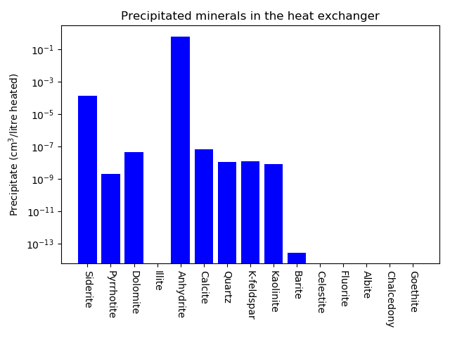
Figure 3: Degree of scaling precipitate expected in the heat exchanger according to the full exchanger-porous_flow-aquifer_geochemistry model.
Results: mineralogy change around the injection well
Minerals precipitate and dissolve around the injection well as shown in Figure 4 and Figure 5. By volume, Illite and Kaolinite undergo most dissolution: indeed, 100% of these minerals are dissolved. In contrast, both K-feldspar and Quartz precipitate. Because the volume of dissolution exceeds the precipitated volume, the porosity increases marginally from its original value of 0.1.
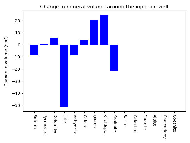
Figure 4: Absolute change of mineral volume around the injection well.
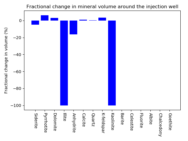
Figure 5: Relative change of mineral volume around the injection well.
Results: 3D contours
Figure 6 shows the results after 90 days of simulation. The input files producing these results employed a fine mesh and set remove_all_extrapolated_secondary_species = true in the GeochemicalModelDefinition to ensure convergence.
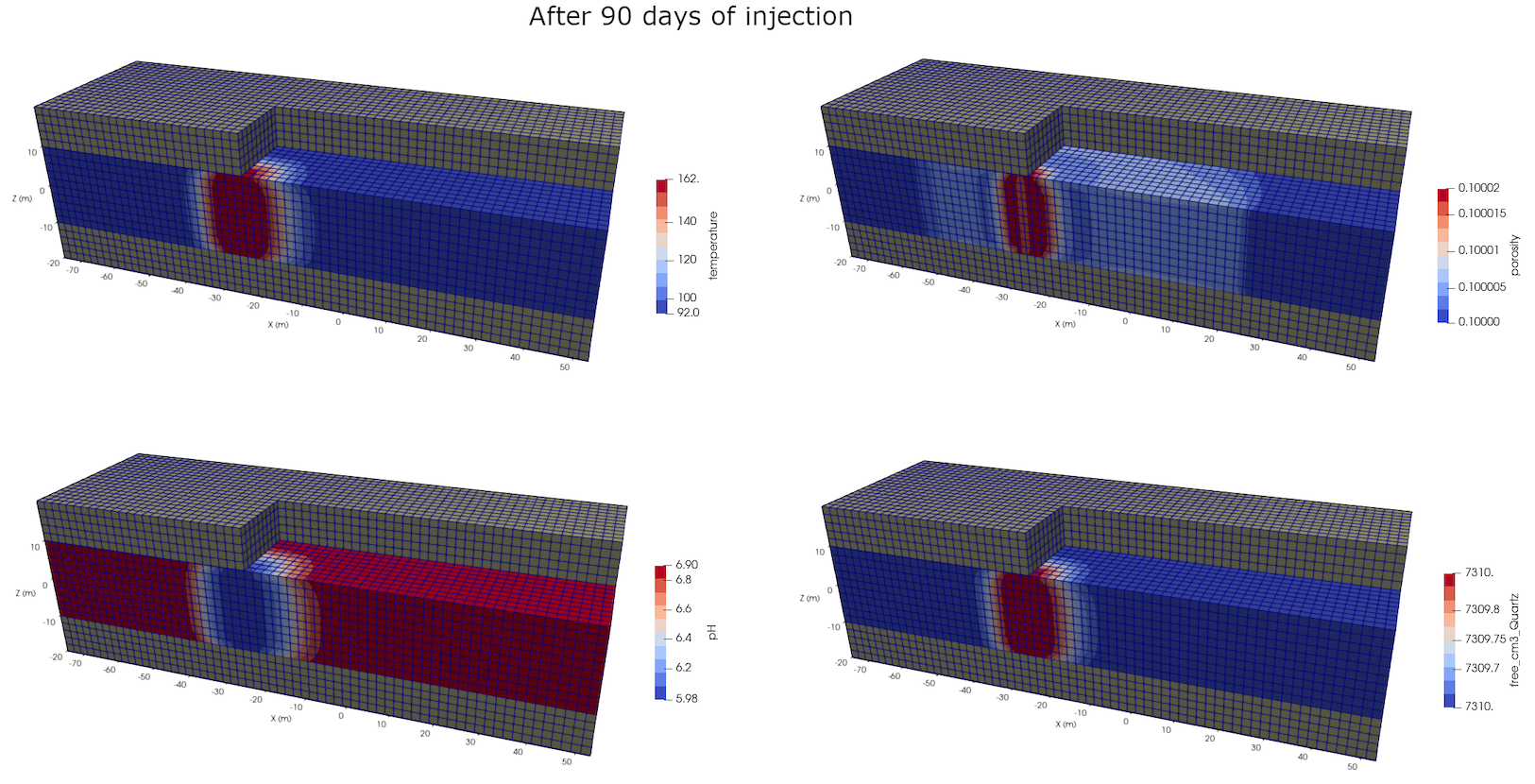
Figure 6: Temperature, porosity, pH and free volume of Quartz after 90 days of injection in the 3D coupled model.
Efficiencies
A related page explores the memory consumption, the impact of linear solver choices and the compute-time scaling with the number of processors of this problem.