Profiling MOOSE code

CPU Profiling

To profile your application, you will need to run a simulation of suitable duration - generally at least a few seconds long - while setting the MOOSE_PROFILE_BASE environment variable to a file base used to store the profiling data. Performing profiling run might look something like this:

MOOSE_PROFILE_BASE=run1_ mpiexec -n 32 ./your-app_oprof -i input_file.i

This will use the filename base you pass and append a suffix of the form [proc#].prof to generate an independent profiling data file for each MPI rank/process. The above example would generate files run1_0.prof, run1_1.prof, run1_2.prof, ..., run1_31.prof. It is allowed to include a directory in the filename base. You can use a command-line argument --gperf-profiler-on with a comma-separated list of MPI ranks to generate the profiling files only on the selected ranks. For example --gperf-profiler-on 0,2 with the above MOOSE_PROFILE_BASE will generate run1_0.prof and run1_2.prof. If this argument is not given, files of all ranks will be generated.

Heap Profiling

Similarly, you can do a heap profiling like this:

HEAP_PROFILE_INUSE_INTERVAL=104857600 MOOSE_HEAP_BASE=run1_ mpiexec -n 32 ./your-app_oprof -i input_file.i

HEAP_PROFILE_INUSE_INTERVAL represents that the code dump heap profiling information whenever the memory usage increases by the specified number of bytes. 104857600 is 100MB. You could choose a small number as well if your simulation does not use much memory. This example should generate files run1_0.xxxx.heap, run1_1.xxxx.heap, run1_2.xxxx.heap, ..., run1_31.xxxx.heap. Here xxxx denotes a sequence number, e.g., 0001 is the first dumped heap file, 0002 is the second dumped heap file, etc. More instructions on heap profiling can be found at here. It is allowed to inclue a directory in the filename base. You can use a command-line argument --gperf-profiler-on with a comma-separated list of MPI ranks to generate the profiling files only on the selected ranks. For example --gperf-profiler-on 0,2 with the above MOOSE_HEAP_BASE will generate run1_0.xxxx.heap and run1_2.xxxx.heap. If this argument is not given, files of all ranks will be generated. This argument can be very useful for reducing the number of profiling files when profiling with a large number of processes.

Analyzing Profile Data

Profiling data can be analyzed using the pprof utility which is included in the latest MOOSE environment package. Or you can also build/install it yourself. When using pprof, the exact same** compiled version of the binary you used to create the profile must** still be located where it was when the profile was created. pprof presents two types of profiling times - "flat" and "cumulative". "flat" times report the amount of time spent directly inside a function (i.e. excluding time spent in transitively called functions), and "cumulative" times report the complete amount of time spent in a function including its descendants (i.e. other functions called by the function transitively).

pprof has an interactive mode accessed by passing a profiling file to the command: pprof run1.prof. In interactive mode, you can run several commands to interrogate the profiling data. A few of these commands are described below, but there are others and several options you can see by entering help or help <cmd|option> in interactive mode or by running pprof --help on the command line. The following sections assume you are running in pprof's interactive mode. We demonstrate the usage of pprof for CPU profiling as follows, and the exact same command lines can applied to heap files as well.

top N

top [N] shows the top N functions that used the most "flat" time:

pprof run1.prof
(pprof) top 12
Showing nodes accounting for 2030ms, 31.92% of 6360ms total
Dropped 362 nodes (cum <= 31.80ms)
Showing top 12 nodes out of 313
      flat  flat%   sum%        cum   cum%
     260ms  4.09%  4.09%      260ms  4.09%  (anonymous namespace)::fe_lagrange_1D_shape
     230ms  3.62%  7.70%      250ms  3.93%  libMesh::DofObject::start_idx
     210ms  3.30% 11.01%      240ms  3.77%  std::_Rb_tree::_M_lower_bound
     200ms  3.14% 14.15%      430ms  6.76%  MooseVariableData::computeValues
     200ms  3.14% 17.30%      200ms  3.14%  libMesh::Elem::active
     170ms  2.67% 19.97%      170ms  2.67%  FEProblemBase::setNeighborSubdomainID
     150ms  2.36% 22.33%      240ms  3.77%  _int_malloc
     140ms  2.20% 24.53%      150ms  2.36%  libMesh::Elem::which_child_am_i
     130ms  2.04% 26.57%      130ms  2.04%  std::vector::size
     120ms  1.89% 28.46%      120ms  1.89%  std::vector::operator[] (inline)
     110ms  1.73% 30.19%      200ms  3.14%  _int_free
     110ms  1.73% 31.92%      220ms  3.46%  libMesh::Elem::level
(pprof)

svg and png

svg and png create a visual profiling graph showing function call relationships and time spent in each function. This is one of the most useful ways to look at the profiling data. The output is printed to screen by default - so you will want to redirect it to a file:

pprof run1.prof
(pprof) png > run1.png

This will create an image like this:

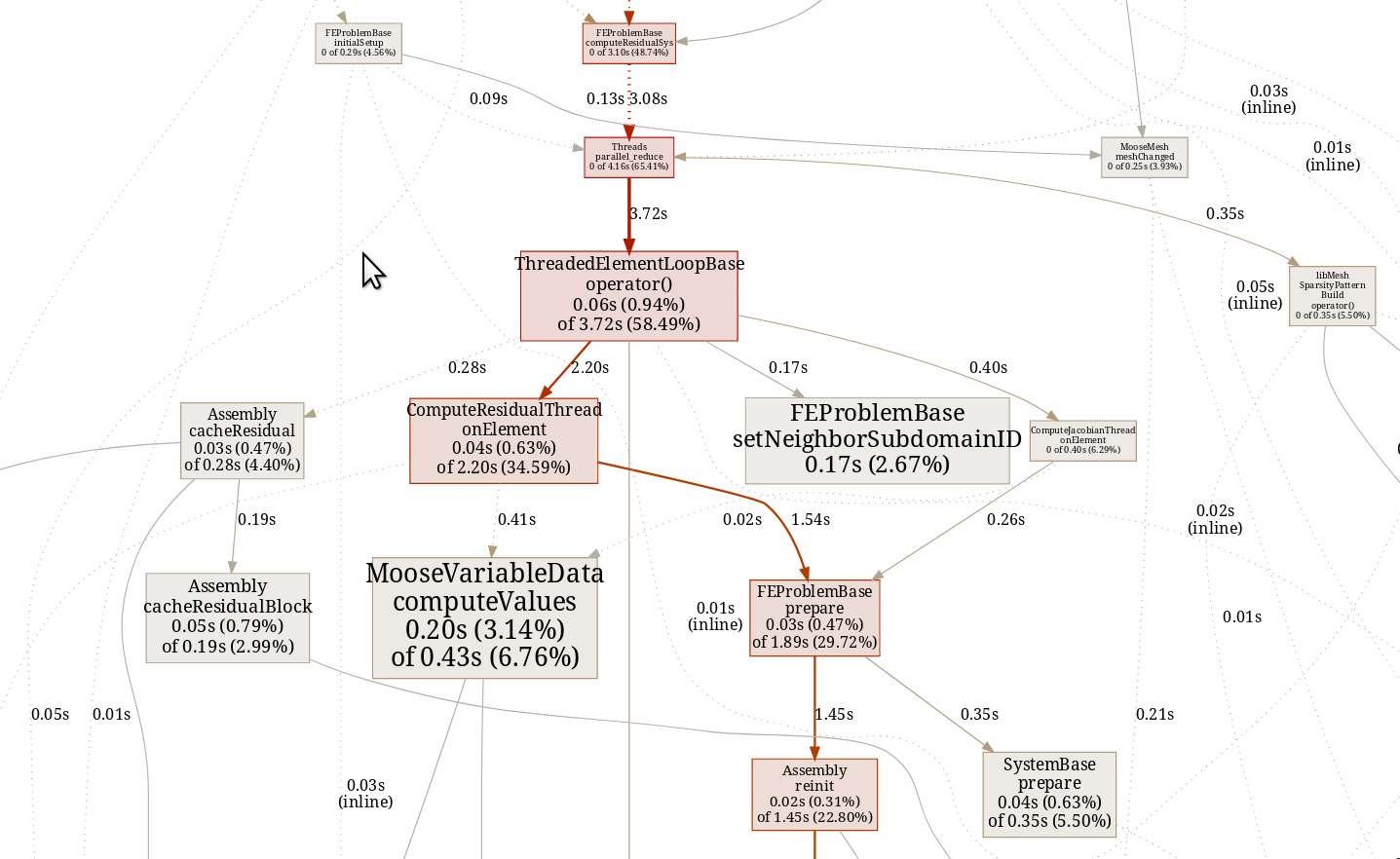
A few notes about data represented in the image:

• Each function is represented by a box/node.

• Boxes include two times/percentages: an upper one for "flat" time and a lower one for "cumulative" time with percentages of total runtime represented by each.

• Each arrow represents a function call.

• Arrows pointing from function A to function B are labeled with "cumulative" time spent in function B that resulted from being called by function A.

• The more red a box/arrow is, the more "cumulative" time is spent in that function/path.

• The larger a box is, the more "flat" time that function takes.

list

list [function-name] shows the code of a function line-by-line side-by-side with both "flat" and "cumulative" time spent on each line:

pprof run1.prof
(pprof) list Assembly::reinit
ROUTINE ======================== Assembly::reinit in /home/calsrw/animals/moose/framework/src/base/Assembly.C
     180ms      5.47s (flat, cum) 21.65% of Total
         .          .   1627:  _current_physical_points = physical_points;
         .          .   1628:}
         .          .   1629:
         .          .   1630:void
         .          .   1631:Assembly::reinit(const Elem * elem)
      50ms       50ms   1632:{
         .          .   1633:  _current_elem = elem;
         .          .   1634:  _current_neighbor_elem = nullptr;
         .          .   1635:  mooseAssert(_current_subdomain_id == _current_elem->subdomain_id(),
         .          .   1636:              "current subdomain has been set incorrectly");
         .          .   1637:  _current_elem_volume_computed = false;
         .          .   1638:
     110ms      120ms   1639:  unsigned int elem_dimension = elem->dim();
         .          .   1640:
         .       30ms   1641:  _current_qrule_volume = _holder_qrule_volume[elem_dimension];
         .          .   1642:
         .          .   1643:  // Make sure the qrule is the right one
         .          .   1644:  if (_current_qrule != _current_qrule_volume)
         .          .   1645:    setVolumeQRule(_current_qrule_volume, elem_dimension);
         .          .   1646:
         .      5.02s   1647:  reinitFE(elem);
         .          .   1648:
         .      230ms   1649:  computeCurrentElemVolume();
      20ms       20ms   1650:}

Newer versions of MacOS (Mojave):

instruments -t Time\ Profiler ./mooseapp-oprof -i input.i

This will create a directory instrumentscli[0-9]+.trace, where [0-9]+ denotes a number, which you can open using

open instrumentscli[0-9]+.trace

The Instruments application will open in a new window with the profile.

Older versions of MacOS (Sierra)

iprofiler -timeprofiler -T 10m ./mooseapp-oprof -i input.i

This will create a directory mooseapp-oprof.dtps which you can open using

open mooseapp-oprof.dtps

The Instruments application will open in a new window with the profile.