SubChannel Theory
Introduction
The diversity of the reactor Gen-IV designs necessitates design, maintenance and support (M&S) software that permits flexible multi-physics capabilities. MOOSE, the Multi-physics Object Oriented Simulation Environment, a parallel computational framework targeted at the solution of coupled, nonlinear partial differential equations (PDEs) that often arise in simulation of nuclear processes. The main advantage of the MOOSE framework is that its a flexible finite element and finite volumes tool in which multiple physics solvers can naturally be coupled. Gen-IV reactors present a significant challenge in their analysis due to their complexity, innovations, and new design features ensuring physics-based passive safety notably. Developing novel nuclear reactor designs and ensuring their safety under normal operating conditions, operational transients, anticipated operational occurrences, design basis accidents (DBA) etc. required the development of novel computational tools. These codes solve the various physics related to nuclear reactors. Neutronics, fuel performance, and thermal-hydraulics, form the primary set of physics that needs to be resolved.
Subchannel codes are thermal-hydraulic codes that offer an efficient compromise for the simulation of a nuclear reactor core, between CFD and system codes. They use a quasi-3D model formulation and allow for a finer mesh than system codes without the high computational cost of CFD. That's why thermal-hydraulic analysis of a nuclear reactor core is often performed using the subchannel type of codes to estimate the various thermal-hydraulic safety margins and the various quantities of interest. The safety margins and the operating power limits of the nuclear reactor core under different conditions, i.e., system pressure, coolant inlet temperature, coolant flow rate, thermal power, and their distributions are considered as the key parameters for subchannel analysis Sha (1980).
Governing Equations
The subchannel thermal-hydraulic analysis is based on the conservation equations of mass, linear momentum and energy on the specified control volumes. The control volumes are connected in both axial and radial directions to capture the three dimensional effects of the flow geometry. The subchannel control volumes are shown in Figure 1 from Todreas et al. (2021).
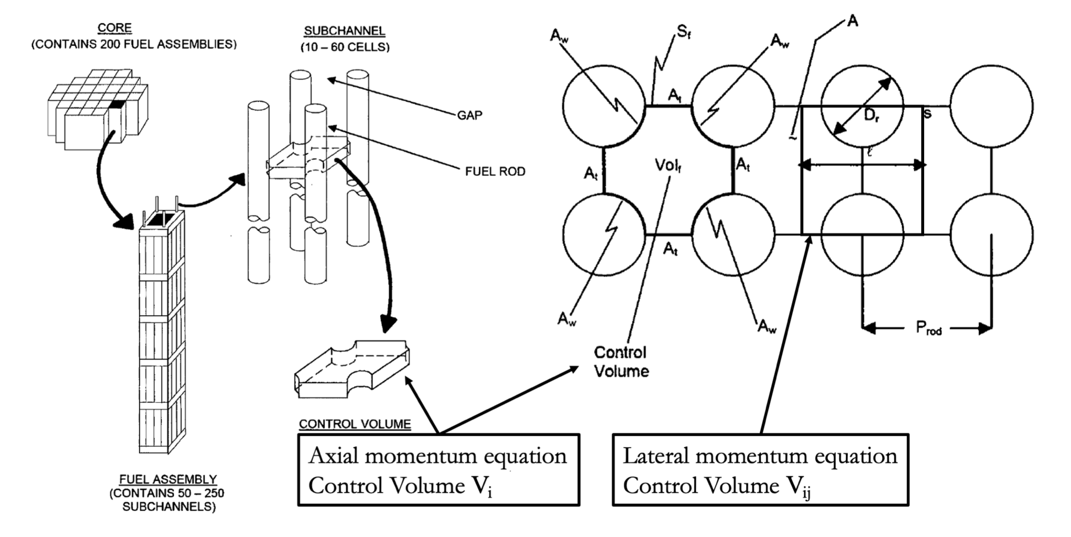
Figure 1: Square Lattice subchannel control volume
The subchannel equations are derived by integrating and averaging the conservation equations over the subchannel control volumes.
Mass conservation equation
(1)
where i is the subchannel index and j the index of the neighbor subchannel. refers to the difference between the inlet and outlet of the control volume in the axial direction. is the mass flow rate of subchannel i in the axial direction. is the diversion crossflow in the lateral direction from subchannel i to neighboring subchannel j, resulting from local pressure differences between the two subchannels.
Axial momentum conservation equation
(2)
In addition to the temporal term in the left hand side there is the change of momentum in the axial direction and the inertia transfer between subchannels due to diversion crossflow . is the axial velocity of the donor cell and represents the gravity force, where is the acceleration of gravity. It is assumed that gravity is the only significant body force in the axial momentum equation. The donor cell is the cell from which crossflow flows out of and depends on the sign of . If it is positive, the donor cell is i and if it is negative, the donor cell is j. Henceforward donor cell quantities will be denoted with the star () symbol. is caused by fluid/pin interface and may also include possible local form loss due to spacers/mixing-vanes. is caused by viscous stresses at the interface between subchannels i and j.
Lateral momentum conservation equation
(3)
Here is the gap between subchannels i,j and the height of the control volume. Lateral pressure gradient () across the subchannels and/or forced mixing between subchannels owing to mixing vanes and spacer grids is the driving force behind diversion crossflow . is the distance between the centers of subchannels i,j. is the average axial velocity of the two subchannels. The overall friction loss term encompasses all the viscous effects and form losses associated with momentum exchange between the fluid and the wall due to the fluid motion through the gap.
Enthalpy conservation equation
(4)
For a single-phase fluid, dissipation due to viscous stresses can be neglected and the total derivative of pressure (work of pressure) set to zero. Also there is no volumetric heat source due to moderation since heat is mainly transferred to the fluid through the fuel pins surface. is the turbulent enthalpy transfer between subchannels i,j and is the average linear power going into the control volumes of subchannel i from the fuel pins.
Closure Models
Axial direction friction term
where is an overall axial loss coefficient encompassing local concentrated form losses due to the changing of the flow area or due to the narrowing of the surface area and frictional losses due to fluid/pin interaction. is the axial flow area, is the Darcy friction factor and is the hydraulic diameter.
Lateral direction friction term
where is an overall loss coefficient encompassing lateral concentrated form and friction losses and the lateral flow area between subchannel i and subchannel j: , is the donor cell density.
Friction factor
The MATRA based friction factor for assemblies with bare pins in a quadrilateral lattice Pang (2014) is presented below. For Reynolds number ranges below , where the MATRA correlation is not applicable, SCM applies a custom extension that keeps the friction factor continuous at the transition to the MATRA correlation:
Additional friction factor models are implemented as follows:
Quadrilateral assembly with bare pins: Chapter 9.6 Pressure drop in rod bundles Todreas and Kazimi (2021).
Triangular assembly with bare pins: Chapter 9.6 Pressure drop in rod bundles Todreas and Kazimi (2021), The upgraded Cheng and Todreas correlation for pressure drop in hexagonal wire-wrapped rod bundles Chen et al. (2018).
Triangular assembly with wire-wrapped pins: Chapter 9.6 Pressure drop in rod bundles Todreas and Kazimi (2021), The upgraded Cheng and Todreas correlation for pressure drop in hexagonal wire-wrapped rod bundles Chen et al. (2018).
Turbulent momentum transfer
The transfer of axial momentum due to turbulence is modelled as follows:
where is a turbulent modeling parameter.
Turbulent enthalpy transfer
The transfer of enthalpy due to turbulence is modelled as follows:
Turbulent crossflow
where is the turbulent mixing parameter or thermal transfer coefficient and is the average mass flux of the adjacent subchannels. The term is the tuning parameter for the mixing model. Physically, it is a non-dimensional coefficient that represents the ratio of the lateral mass flux due to mixing to the axial mass flux. It is used to model the effect of the unresolved scales of motion that are produced through the averaging process. In single-phase flow no net mass exchange occurs, both momentum and energy are exchanged between subchannels, and their rates of exchange are characterized in terms of hypothetical turbulent interchange flow rates () Todreas et al. (2021), for enthalpy and momentum respectively. For this unresolved turbulent interchange model, the approximation that the rate of turbulent exchange for energy and momentum are related as follows is adopted: .
The mixing closure provides only this unresolved turbulent interchange coefficient. Friction closures enter the axial and lateral momentum equations through the pressure-drop terms, and heat-transfer closures enter the energy equation through pin/duct heat addition. When a mixing closure requires local flow information such as a friction factor, the selected friction closure is used internally by that empirical mixing correlation; otherwise is coupled to the governing equations only through and the optional momentum scaling above.
Sweep flow
The turbulent interchange relation above is not applicable to wire-wrap sweep flow. In wire-wrapped triangular assemblies, sweep flow represents a directed peripheral enthalpy transport induced by the wire wrap. SCM applies the sweep-flow coefficient only in the triangular-assembly energy equation, where the term transports enthalpy between edge and corner subchannels. It is not included in the momentum exchange term and is not scaled by ; equivalently, SCM does not currently model a corresponding momentum sweep-flow closure.
Additional turbulent mixing parameters are implemented as follows:
Quadrilateral assembly with bare pins: A scale analysis of the turbulent mixing rate for various Prandtl number flow fields in rod bundles eq 25,Kim and Chung (2001) Kim and Chung (2001), Modeling of flow blockage in a liquid metal-cooled reactor subassembly with a subchannel analysis code eq 19, Jeong et. al (2005)Jeong et al. (2005).
Triangular assembly with bare pins: A scale analysis of the turbulent mixing rate for various Prandtl number flow fields in rod bundles eq 25,Kim and Chung (2001) Kim and Chung (2001).
Triangular assembly with wire-wrapped pins: Hydrodynamic models and correlations for bare and wire-wrapped hexagonal rod bundles—bundle friction factors, subchannel friction factors and mixing parameters, Cheng and Todreas Cheng and Todreas (1986).
Calibrated parameter values
has been calibrated for quadrilateral assemblies using data from the 2x3 air-water facility that was operated by Kumamoto university. The purpose of that facility was to quantify the effects of mixing and void drift Sadatomi et al. (2004). In these experiments, the turbulent mixing rates and the fluctuations of static pressure difference between subchannels were measured. The author derived a way to use the die concentration measurements, in order to calculate the turbulent mixing rates () between subchannels Kawahara et al. (1995).
It is important to note that the mixing coefficient is simply a tuning parameter that will depend on the specific geometry of the facility being modeled. This facility is a square lattice, but the geometry is much larger than that of a typical PWR pin-lattice geometry. Nevertheless this study is useful for showing that the code is capable of predicting the correct mixing rate if it is calibrated correctly.
After calibrating the turbulent diffusion coefficient we turned our attention to the turbulent modeling parameter . This is a tuning parameter that informs on how much momentum is transferred/diffused between subchannels, due to turbulence. The CNEN 4x4 test Marinelli et al. (1972) performed at Studsvik laboratory for studying the flow mixing effect between adjacent subchannels was chosen to tune this parameter. This experiment consists in velocity and temperature measurements taken at the outlet of a 16-pin assembly test section. Analysis of the velocity distribution at the exit of the assembly can be used to calibrate the turbulent parameter .
For quadrilateral assemblies: , Kyriakopoulos et al. (2022).
Discretization
The collocated discretization of the variables is presented in Figure 2 . are the subchannel indexes. is the name of the gap between subchannels . is the index in the axial direction.
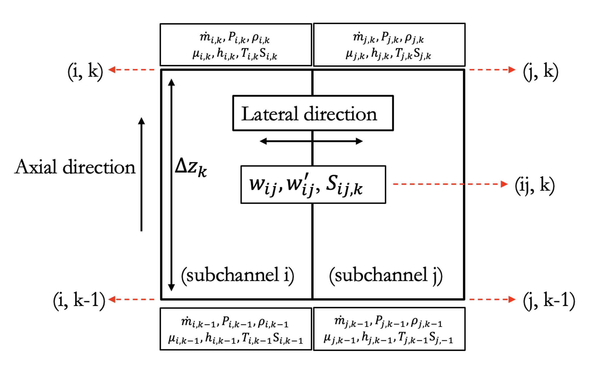
Figure 2: Subchannel collocated discretization.
The governing equations are discretized as follows:
Conservation of mass:
(5)
- The above equation can be written in matrix form as follows:
which is equivalent to:
(6)
Similarly for the other equations,
Conservation of linear momentum in the axial direction:
(7) and in matrix form, (8)
where the matrix is calculated using the lagged values of the unknown variables .
Conservation of linear momentum in the lateral direction:
(9)
The above equation can be written in matrix form as follows: (10) where the matrix is calculated using the lagged values of the unknown variables .
Conservation of enthalpy:
(11)
The above equation can be written in matrix form as follows:
(12) where the matrix is calculated using the lagged values of the unknown variables .
Algorithm
A hybrid numerical method of solving the subchannel equations was developed. Hybrid in this context means that the user has the option of solving each portion of the problem at a time, by dividing the domain into blocks. Each block is solved sequentially from inlet to outlet. The mass flow at the outlet of the previous block and the pressure at the inlet of the next block provide the needed boundary conditions. The essence of the algorithm hinges on the construction of a combined residual function based on the lateral momentum equation. To solve this equation a Jacobian Free Newton-Krylov type Method (JFNKM) was used. The workhorse of the code is the non linear equation solvers (SNES) found in the Portable, Extensible Toolkit for Scientific Computation PETSc.
(13)
The main unknown variable in this non linear residual is the crossflow . The combined residual function calculates the non linear residual after it updates the other main flow variables, such as mass flow , turbulent crossflow , pressure drop and pressure , using the current as needed. So every time this function is called by the Newton solver the flow variables get updated. This affords the solution of all flow variables at the same time. is the local pressure minus the exit pressure, , so at the exit is zero. The hybrid algorithm is presented in Figure 3.
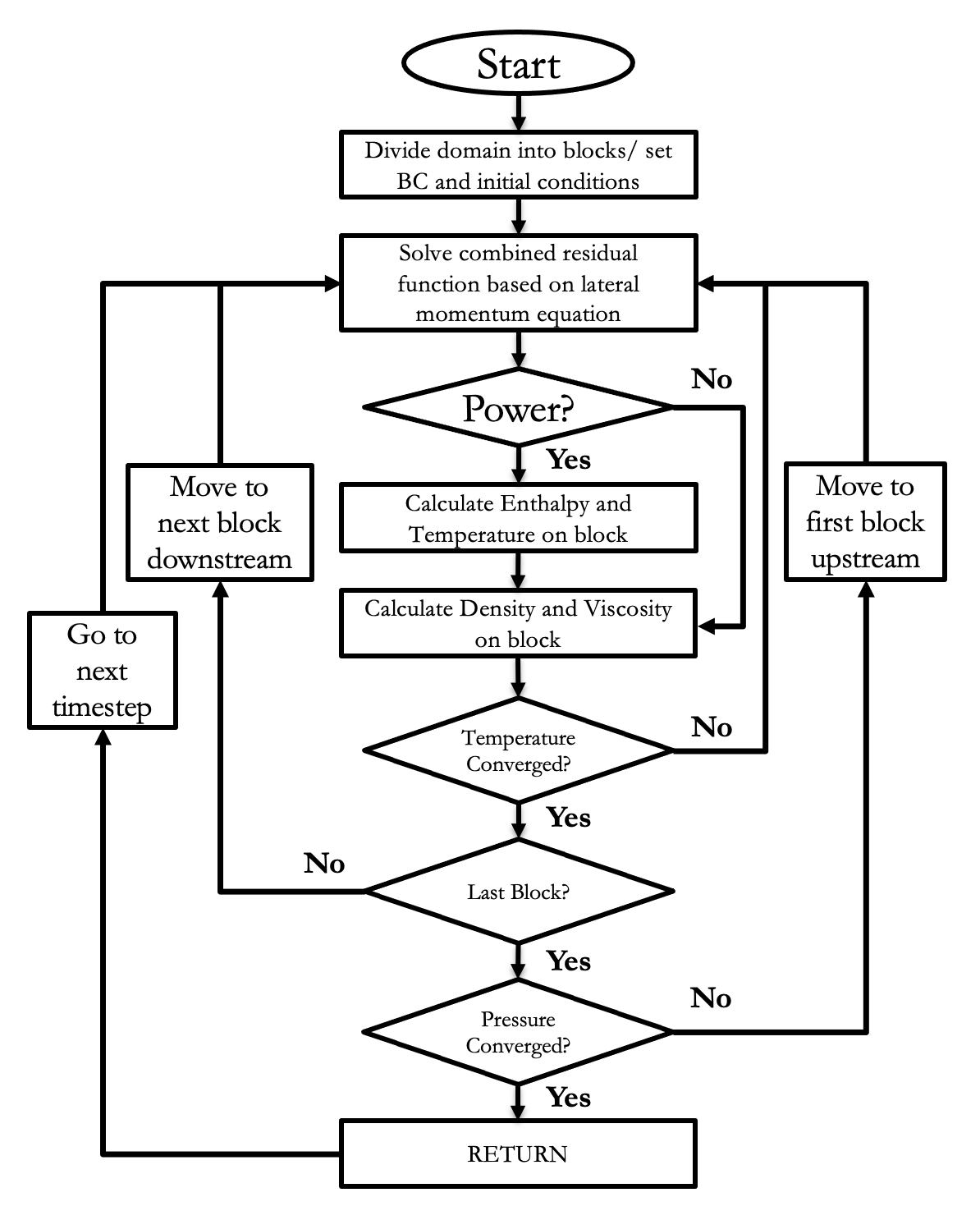
Figure 3: SCM hybrid numerical scheme
Once the main flow variables converge in a block, the enthalpy conservation equation is solved and enthalpy is retrieved in all the nodes of the block. In the special case where no heat is added to the fluid in the block, the enthalpy does not need to be calculated in that block (unless there is a non-uniform enthalpy inlet distribution). Using enthalpy, pressure and the equations of state, temperature and the fluid properties such as density and viscosity are calculated. After the fluid properties are updated, the solve is repeated until the temperature field converges. Once the temperature solution converges the procedure is repeated for the next block downstream. Once the temperature solution converges in all blocks we check to see if pressure has converged in all blocks. If not, we repeat the procedure starting again from the first block, until pressure has converged. Note that in order for the pressure information from the outlet to reach the inlet, it will require a number of the pressure loop iterations equal to the number of blocks. Last, the calculation of the flow variables and of the residual is done in an explicit manner.
Algorithm variations
There are three variations Kyriakopoulos and Tano (2026) of the algorithm presented above in SCM: The Explicit-Segregated, Implicit-Segregated and Monolithic. There are also two subchannel geometries that SCM can solve, one with fuel pins in a quadrilateral lattice (Quadsolver) and one with fuel pins in a triangular lattice (Trisolver). There should be no appreciable differences between the results of the algorithms when the time/spacial discretization scheme is converged.
Explicit-Segregated
This is the default algorithm, where the unknown flow variables are calculated in an explicit manner through their governing equations. The variables are updated sequantially from block inlet to block outlet except for pressure which is updated from block outlet to block inlet. Blocks are solved sequentially from assembly inlet to assembly outlet.
Implicit-Segregated
In this case, the governing mass, axial momentum and crossflow momentum, equations are recast in matrix form and the flow variables are calculated by solving the corresponding system. This means that variables are retrieved concurrently for the whole block. Otherwise, the solution algorithm is the same as in the default explicit method.
Monolithic
In this case, the governing mass, axial momentum and crossflow momentum conservation equations are recast in matrix form and combined into a single system. The system of all the subchannel equations looks like this:
Since the enthalpy governing equations are uncoupled from the other equations in this otherwise monolithic system (enthalpy is coupled to the flow equations via the fluid properties update), it makes sense to lag the enthalpy solution and solve for it separately. The flow variables are calculated by solving that big system (without the enthalpy) to retrieve all the unknowns at the same time instead of one by one, and on all the nodes of the block: is not explicitly calculated, otherwise the solution algorithm is the same as in the default method and the solver used is PETSc KSPSolve.
As soon as the big matrix is constructed, the solver will calculate cross-flow resistances to maintain realizability. A distinctive feature of this method is the introduction of a weak relaxation logic that stabilizes and accelerates convergence of the coupled , , and fields in a block-nested linear system with matrix blocks and right-hand-side blocks that represent the individual governing equations. Note that the solution is influenced by the stabilization method and its coefficients.
1. Fast scale estimates
From the axial- and cross-momentum rows, the code forms quick, diagonally preconditioned estimates: with small safeguards to avoid division by zero. Using , the per-channel crossflow sum is assembled into a vector .
2. Crossflow relaxation parameter
Two guarded scalars are computed:
Additionally, a mean inter-iteration change for crossflow is formed leading to a relaxation factor The +0.5 offset biases toward mild under-relaxation.
3. Crossflow resistance inflation
A cross-coupling resistance is estimated and smoothed: After smoothing, the provisional crossflow resistance is mapped through a piecewise lower-bound function that enforces minimum safe damping levels in specific ranges.
This mapping acts as a {snap-up} rule for the crossflow resistance over the range : it raises out of weak-damping intervals but leaves very small and very large values unchanged. The purpose is to maintain numerical stability and adequate diagonal dominance in the cross-momentum equations without introducing full quantization or "bucketing".
Finally, is added to the diagonal of the cross-momentum block, thereby increasing diagonal dominance and improving conditioning for the crossflow equations. Note that this treatment does influence the cross-flow distribution solution.
4. Per-equation under-relaxation
Classical linear under-relaxation is applied automatically and separately to each equation using factors For each equation, with the corresponding diagonal , the system is modified as This standard construction ensures that solving the modified linear system yields the under-relaxed update for equation . In practice, only is strongly damped, while and can be solved without additional damping. This relaxation happens inside the temperature loop.
5. Net effect
The combination of (i) safeguarded scale estimation, (ii) adaptive, time smoothed, and piecewise snapped added crossflow resistance, and (iii) selective under-relaxation produces a more diagonally dominant and robust nested solve that tolerates rapid changes in crossflow while preserving good convergence properties for mass flow and pressure.
References
- SK Chen, YM Chen, and NE Todreas.
The upgraded cheng and todreas correlation for pressure drop in hexagonal wire-wrapped rod bundles.
Nuclear Engineering and Design, 335:356–373, 2018.[Export]
- Shih-Kuei Cheng and Neil E Todreas.
Hydrodynamic models and correlations for bare and wire-wrapped hexagonal rod bundles—bundle friction factors, subchannel friction factors and mixing parameters.
Nuclear engineering and design, 92(2):227–251, 1986.[Export]
- Hae-Yong Jeong, Kwi-Seok Ha, Won-Pyo Chang, Young-Min Kwon, and Yong-Bum Lee.
Modeling of flow blockage in a liquid metal-cooled reactor subassembly with a subchannel analysis code.
Nuclear technology, 149(1):71–87, 2005.[Export]
- Akimaro Kawahara, Michio Sadatomi, Yoshifusa Sato, and Eiichi Shiga.
Treatment of turbulent mixing rate in a two-phase subchannel flow. for developing flow without pressure differential between subchannels.
Nippon Kikai Gakkai Ronbunshu, B Hen, 61(583):861–867, 1995.[Export]
- Sin Kim and Bum-Jin Chung.
A scale analysis of the turbulent mixing rate for various prandtl number flow fields in rod bundles.
Nuclear engineering and design, 205(3):281–294, 2001.[Export]
- Vasileios Kyriakopoulos and Mauricio Tano.
Numerical implementation of the moose subchannel module (scm) algorithm.
Nuclear Engineering and Design, 450:114802, 2026.[Export]
- Vasileios Kyriakopoulos, Mauricio E Tano, and Jean C Ragusa.
Development of a single-phase, transient, subchannel code, within the moose multi-physics computational framework.
Energies, 15(11):3948, 2022.[Export]
- V Marinelli, L Pastori, and B Kjellen.
Experimental investigation on mass velocity distribution and velocity profiles in an lwr rod bundle.
Trans. Amer. Nucl. Soc., 15(1):413, 1972.[Export]
- Bo Pang.
Numerical study of void drift in pin bundle with subchannel and CFD codes.
Volume 7669.
KIT Scientific Publishing, 2014.[Export]
- M. Sadatomi, A. Kawahara, K. Kano, and Y. Sumi.
Single- and two-phase turbulent mixing rate between adjacent subchannels in a vertical 2x3 rod array channel.
International Journal of Multiphase Flow, 30(5):481–498, 2004.[Export]
- William T. Sha.
An overview on pin-bundle thermal-hydraulic analysis.
Nuclear Engineering and Design, 62(1):1–24, 1980.
URL: https://www.sciencedirect.com/science/article/pii/0029549380900187, doi:https://doi.org/10.1016/0029-5493(80)90018-7.[Export]
- Neil E Todreas and Mujid S Kazimi.
Nuclear systems volume I: Thermal hydraulic fundamentals.
CRC press, 2021.[Export]
- Neil E Todreas, Mujid S Kazimi, and Mahmoud Massoud.
Nuclear systems Volume II: Elements of thermal hydraulic design.
CRC Press, 2021.[Export]