Heat advection in a 1D bar
Consider the case of a single-phase fluid in 1 dimension, , with the porepressure fixed at the boundaries: With zero gravity, and high fluid bulk modulus, the Darcy equation implies that the solution is , with being the constant "Darcy velocity" from to . (The velocity of the individual fluid particles, this is divided by the porosity.). Here is the porous medium's permeability, and is the fluid dynamic viscosity.
Suppose that the fluid internal energy is given by , where is the specific heat capacity and is its temperature. Assuming that , then the fluid's enthalpy is also . In this case, the energy equation reads This is the wave equation with velocity Recall that the "Darcy velocity" is .
Let the initial condition for be . Apply the boundary conditions At this creates a front at . Choose the parameters , , , , , , (all in consistent units), so that is the front's velocity.
The input file used in this page is:
# 1phase, heat advecting with a moving fluid
# Using the PorousFlowFullySaturated Action with various stabilization options
# With stabilization=none, this should produce an identical result to heat_advection_1d_fully_saturated.i
# With stabilization=Full, this should produce an identical result to heat_advection_1d.i and heat_advection_1d_fullsat.i
# With stabilization=KT, this should produce an identical result to heat_advection_1D_KT.i
[Mesh<<<{"href": "../../../../syntax/Mesh/index.html"}>>>]
  type = GeneratedMesh
  dim = 1
  nx = 50
  xmin = 0
  xmax = 1
[]

[GlobalParams<<<{"href": "../../../../syntax/GlobalParams/index.html"}>>>]
  PorousFlowDictator = dictator
  gravity = '0 0 0'
[]

[Variables<<<{"href": "../../../../syntax/Variables/index.html"}>>>]
  [temp]
    initial_condition<<<{"description": "Specifies a constant initial condition for this variable"}>>> = 200
  []
  [pp]
  []
[]

[ICs<<<{"href": "../../../../syntax/ICs/index.html"}>>>]
  [pp]
    type = FunctionIC<<<{"description": "An initial condition that uses a normal function of x, y, z to produce values (and optionally gradients) for a field variable.", "href": "../../../../source/ics/FunctionIC.html"}>>>
    variable<<<{"description": "The variable this initial condition is supposed to provide values for."}>>> = pp
    function<<<{"description": "The initial condition function."}>>> = '1-x'
  []
[]

[BCs<<<{"href": "../../../../syntax/BCs/index.html"}>>>]
  [pp0]
    type = DirichletBC<<<{"description": "Imposes the essential boundary condition $u=g$, where $g$ is a constant, controllable value.", "href": "../../../../source/bcs/DirichletBC.html"}>>>
    variable<<<{"description": "The name of the variable that this residual object operates on"}>>> = pp
    boundary<<<{"description": "The list of boundary IDs from the mesh where this object applies"}>>> = left
    value<<<{"description": "Value of the BC"}>>> = 1
  []
  [pp1]
    type = DirichletBC<<<{"description": "Imposes the essential boundary condition $u=g$, where $g$ is a constant, controllable value.", "href": "../../../../source/bcs/DirichletBC.html"}>>>
    variable<<<{"description": "The name of the variable that this residual object operates on"}>>> = pp
    boundary<<<{"description": "The list of boundary IDs from the mesh where this object applies"}>>> = right
    value<<<{"description": "Value of the BC"}>>> = 0
  []
  [spit_heat]
    type = DirichletBC<<<{"description": "Imposes the essential boundary condition $u=g$, where $g$ is a constant, controllable value.", "href": "../../../../source/bcs/DirichletBC.html"}>>>
    variable<<<{"description": "The name of the variable that this residual object operates on"}>>> = temp
    boundary<<<{"description": "The list of boundary IDs from the mesh where this object applies"}>>> = left
    value<<<{"description": "Value of the BC"}>>> = 300
  []
  [suck_heat]
    type = DirichletBC<<<{"description": "Imposes the essential boundary condition $u=g$, where $g$ is a constant, controllable value.", "href": "../../../../source/bcs/DirichletBC.html"}>>>
    variable<<<{"description": "The name of the variable that this residual object operates on"}>>> = temp
    boundary<<<{"description": "The list of boundary IDs from the mesh where this object applies"}>>> = right
    value<<<{"description": "Value of the BC"}>>> = 200
  []
[]

[PorousFlowFullySaturated<<<{"href": "../../../../syntax/PorousFlowFullySaturated/index.html"}>>>]
  porepressure<<<{"description": "The name of the porepressure variable"}>>> = pp
  temperature<<<{"description": "For isothermal simulations, this is the temperature at which fluid properties (and stress-free strains) are evaluated at.  Otherwise, this is the name of the temperature variable.  Units = Kelvin"}>>> = temp
  coupling_type<<<{"description": "The type of simulation.  For simulations involving Mechanical deformations, you will need to supply the correct Biot coefficient.  For simulations involving Thermal flows, you will need an associated ConstantThermalExpansionCoefficient Material"}>>> = ThermoHydro
  fp<<<{"description": "The name of the user object for fluid properties. Only needed if fluid_properties_type = PorousFlowSingleComponentFluid"}>>> = simple_fluid
  add_darcy_aux<<<{"description": "Add AuxVariables that record Darcy velocity"}>>> = false
  stabilization<<<{"description": "Numerical stabilization used.  'Full' means full upwinding.  'KT' means FEM-TVD stabilization of Kuzmin-Turek"}>>> = none
  flux_limiter_type<<<{"description": "Type of flux limiter to use if stabilization=KT.  'None' means that no antidiffusion will be added in the Kuzmin-Turek scheme"}>>> = superbee
[]

[FluidProperties<<<{"href": "../../../../syntax/FluidProperties/index.html"}>>>]
  [simple_fluid]
    type = SimpleFluidProperties<<<{"description": "Fluid properties for a simple fluid with a constant bulk density", "href": "../../../../source/fluidproperties/SimpleFluidProperties.html"}>>>
    bulk_modulus<<<{"description": "Constant bulk modulus (Pa)"}>>> = 100
    density0<<<{"description": "Density at zero pressure and zero temperature"}>>> = 1000
    viscosity<<<{"description": "Constant dynamic viscosity (Pa.s)"}>>> = 4.4
    thermal_expansion<<<{"description": "Constant coefficient of thermal expansion (1/K)"}>>> = 0
    cv<<<{"description": "Constant specific heat capacity at constant volume (J/kg/K)"}>>> = 2
  []
[]

[Materials<<<{"href": "../../../../syntax/Materials/index.html"}>>>]
  [porosity]
    type = PorousFlowPorosityConst<<<{"description": "This Material calculates the porosity assuming it is constant", "href": "../../../../source/materials/PorousFlowPorosityConst.html"}>>>
    porosity<<<{"description": "The porosity (assumed indepenent of porepressure, temperature, strain, etc, for this material).  This should be a real number, or a constant monomial variable (not a linear lagrange or other kind of variable)."}>>> = 0.2
  []
  [zero_thermal_conductivity]
    type = PorousFlowThermalConductivityIdeal<<<{"description": "This Material calculates rock-fluid combined thermal conductivity by using a weighted sum.  Thermal conductivity = dry_thermal_conductivity + S^exponent * (wet_thermal_conductivity - dry_thermal_conductivity), where S is the aqueous saturation", "href": "../../../../source/materials/PorousFlowThermalConductivityIdeal.html"}>>>
    dry_thermal_conductivity<<<{"description": "The thermal conductivity of the rock matrix when the aqueous saturation is zero"}>>> = '0 0 0  0 0 0  0 0 0'
  []
  [rock_heat]
    type = PorousFlowMatrixInternalEnergy<<<{"description": "This Material calculates the internal energy of solid rock grains, which is specific_heat_capacity * density * temperature.  Kernels multiply this by (1 - porosity) to find the energy density of the porous rock in a rock-fluid system", "href": "../../../../source/materials/PorousFlowMatrixInternalEnergy.html"}>>>
    specific_heat_capacity<<<{"description": "Specific heat capacity of the rock grains (J/kg/K)."}>>> = 1.0
    density<<<{"description": "Density of the rock grains"}>>> = 125
  []
  [permeability]
    type = PorousFlowPermeabilityConst<<<{"description": "This Material calculates the permeability tensor assuming it is constant", "href": "../../../../source/materials/PorousFlowPermeabilityConst.html"}>>>
    permeability<<<{"description": "The permeability tensor (usually in m^2), which is assumed constant for this material"}>>> = '1.1 0 0 0 2 0 0 0 3'
  []
[]

[Preconditioning<<<{"href": "../../../../syntax/Preconditioning/index.html"}>>>]
  [andy]
    type = SMP<<<{"description": "Single matrix preconditioner (SMP) builds a preconditioner using user defined off-diagonal parts of the Jacobian.", "href": "../../../../source/preconditioners/SingleMatrixPreconditioner.html"}>>>
    full<<<{"description": "Set to true if you want the full set of couplings between variables simply for convenience so you don't have to set every off_diag_row and off_diag_column combination."}>>> = true
  []
[]

[Executioner<<<{"href": "../../../../syntax/Executioner/index.html"}>>>]
  type = Transient
  solve_type = Newton
  dt = 0.01
  end_time = 0.6
[]

[VectorPostprocessors<<<{"href": "../../../../syntax/VectorPostprocessors/index.html"}>>>]
  [T]
    type = LineValueSampler<<<{"description": "Samples variable(s) along a specified line", "href": "../../../../source/vectorpostprocessors/LineValueSampler.html"}>>>
    start_point<<<{"description": "The beginning of the line"}>>> = '0 0 0'
    end_point<<<{"description": "The ending of the line"}>>> = '1 0 0'
    num_points<<<{"description": "The number of points to sample along the line"}>>> = 51
    sort_by<<<{"description": "What to sort the samples by. Options include 'x', 'y', 'z', 'id', and the name of any of the sampled quantities (which each create a vector of the same name)."}>>> = x
    variable<<<{"description": "The names of the variables that this VectorPostprocessor operates on"}>>> = temp
  []
[]

[Outputs<<<{"href": "../../../../syntax/Outputs/index.html"}>>>]
  file_base<<<{"description": "Common file base name to be utilized with all output objects"}>>> = heat_advection_1d_fully_saturation_action
  [csv]
    type = CSV<<<{"description": "Output for postprocessors, vector postprocessors, and scalar variables using comma seperated values (CSV).", "href": "../../../../source/outputs/CSV.html"}>>>
    sync_times<<<{"description": "Times at which the output and solution is forced to occur"}>>> = '0.1 0.6'
    sync_only<<<{"description": "Only export results at sync times"}>>> = true
  []
[]The sharp front is not maintained by MOOSE. This is due to numerical diffusion, whose magnitude depends on the stabilization scheme used. This is explained in great detail in the pages on numerical stabilization. Nevertheless, MOOSE advects the smooth front with the correct velocity, as shown in Figure 1.
Figure 1 shows three versions of the advection, which are activated by setting the stabilization parameter in the PorousFlowFullySaturated Action:
with no stabilization
stabilization = none
with full upwinding
stabilization = Full
with KT stabilization
stabilization = KT
With no numerical stabilization, two additional points may also be noticed: (1) the lack of upwinding has produced a "bump" in the temperature profile near the hotter side; (2) the lack of upwinding means the temperature profile moves slightly slower than it should. These two affects reduce as the mesh density is increased, however.
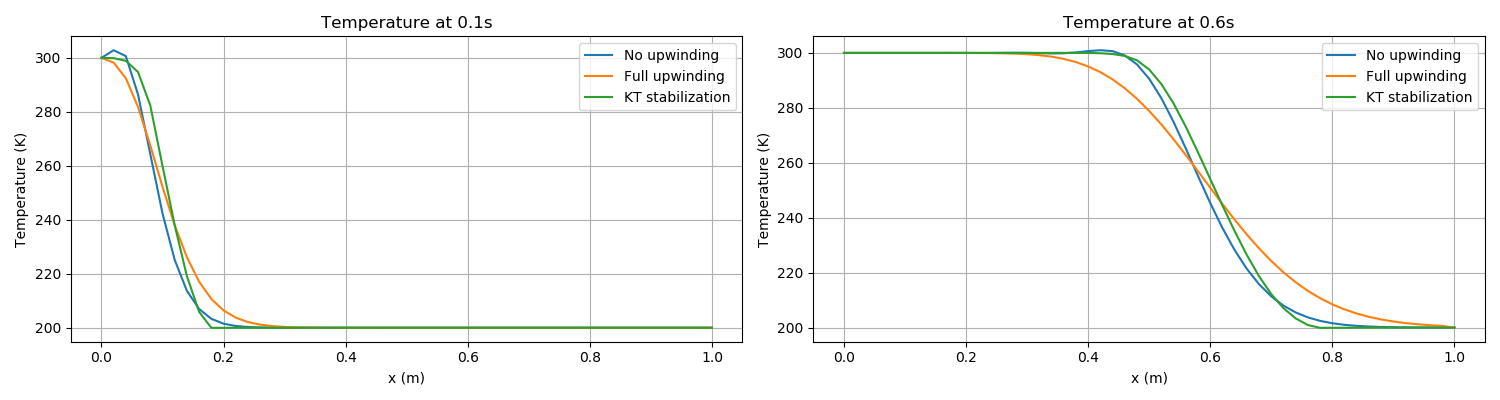
Figure 1: Results of heat advection via a fluid in 1D. The fluid flows with constant Darcy velocity of 0.25m/s to the right, and this advects a temperature front at velocity 1m/s to the right. The pictures above that the numerical implementation of PorousFlow (including upwinding) diffuses sharp fronts, but advects them at the correct velocity (notice the centre of the upwinded front is at the correct position in each picture). Less diffusion is experienced without upwinding or with KT stabilization. Left: temperature 0.1s. Right: temperature at 0.6s.