Dead-oil waterflood
These examples show how to model the injection of water into a reservoir containing dead oil (oil without dissolved gas). The oil properties are read from a table of the type used by black-oil reservoir simulators, so they can be used as a starting point for models that use existing PVT data.
Fluid and rock properties
There are two phases and two components: water (phase 0, component 0) and dead oil (phase 1, component 1). Neither component dissolves in the other phase, which is described by the mass fractions
[AuxVariables<<<{"href": "../../syntax/AuxVariables/index.html"}>>>]
  # Water is entirely in phase 0 and oil is entirely in phase 1
  [frac_water_in_water]
    initial_condition<<<{"description": "Specifies a constant initial condition for this variable"}>>> = 1.0
  []
  [frac_water_in_oil]
    initial_condition<<<{"description": "Specifies a constant initial condition for this variable"}>>> = 0.0
  []
  [swater]
    family<<<{"description": "Specifies the family of FE shape functions to use for this variable"}>>> = MONOMIAL
    order<<<{"description": "Specifies the order of the FE shape function to use for this variable (additional orders not listed are allowed)"}>>> = CONSTANT
  []
[]The water is a SimpleFluidProperties fluid with a viscosity of 0.5mPas. The oil properties are given by TabulatedPVTFluidProperties, using a PVDO-style table of pressure, formation volume factor and viscosity , together with the oil density at standard conditions:
[FluidProperties<<<{"href": "../../syntax/FluidProperties/index.html"}>>>]
  [water]
    type = SimpleFluidProperties<<<{"description": "Fluid properties for a simple fluid with a constant bulk density", "href": "../../source/fluidproperties/SimpleFluidProperties.html"}>>>
    density0<<<{"description": "Density at zero pressure and zero temperature"}>>> = 1000
    bulk_modulus<<<{"description": "Constant bulk modulus (Pa)"}>>> = 2.2e9
    viscosity<<<{"description": "Constant dynamic viscosity (Pa.s)"}>>> = 0.5e-3
    thermal_expansion<<<{"description": "Constant coefficient of thermal expansion (1/K)"}>>> = 0
  []
  # Dead oil, PVDO-style table: pressure (Pa), formation volume factor (rm3/sm3), viscosity (Pa.s)
  [oil]
    type = TabulatedPVTFluidProperties<<<{"description": "Isothermal fluid properties from a table of pressure, formation volume factor and viscosity (PVDO/PVDG style). 1/B and 1/(B mu) are interpolated linearly in pressure.", "href": "../../source/fluidproperties/TabulatedPVTFluidProperties.html"}>>>
    density_sc<<<{"description": "Density of the fluid at standard (surface) conditions (kg/m^3)"}>>> = 850
    pressure<<<{"description": "Tabulated pressures (Pa). Must be strictly increasing"}>>> = '1.0e7 2.0e7 3.0e7'
    formation_volume_factor<<<{"description": "Formation volume factor B (reservoir volume / standard volume) at each tabulated pressure"}>>> = '1.050 1.038 1.028'
    viscosity<<<{"description": "Dynamic viscosity (Pa.s) at each tabulated pressure"}>>> = '1.10e-3 1.17e-3 1.24e-3'
  []
[]The problem is formulated with the water porepressure and the oil saturation as the nonlinear variables, using PorousFlow2PhasePS with zero capillary pressure. The porosity is 0.2, the permeability is m (approximately 1 Darcy), and the relative permeabilities are of Corey type with exponent 2, a connate water saturation of 0.2 and a residual oil saturation of 0.2:
[Materials<<<{"href": "../../syntax/Materials/index.html"}>>>]
  [temperature]
    type = PorousFlowTemperature<<<{"description": "Material to provide temperature at the quadpoints or nodes and derivatives of it with respect to the PorousFlow variables", "href": "../../source/materials/PorousFlowTemperature.html"}>>>
    temperature<<<{"description": "Fluid temperature variable.  Note, the default is suitable if your simulation is using Kelvin units, but probably not for Celsius"}>>> = 350
  []
  [saturation_calculator]
    type = PorousFlow2PhasePS<<<{"description": "This Material calculates the 2 porepressures and the 2 saturations in a 2-phase situation, and derivatives of these with respect to the PorousFlowVariables.", "href": "../../source/materials/PorousFlow2PhasePS.html"}>>>
    phase0_porepressure<<<{"description": "Variable that is the porepressure of phase 0 (the liquid phase)"}>>> = pwater
    phase1_saturation<<<{"description": "Variable that is the saturation of phase 1 (the gas phase)"}>>> = soil
    capillary_pressure<<<{"description": "Name of the UserObject defining the capillary pressure"}>>> = pc
  []
  [massfrac]
    type = PorousFlowMassFraction<<<{"description": "This Material forms a std::vector<std::vector ...> of mass-fractions out of the individual mass fractions", "href": "../../source/materials/PorousFlowMassFraction.html"}>>>
    mass_fraction_vars<<<{"description": "List of variables that represent the mass fractions.  Format is 'f_ph0^c0 f_ph0^c1 f_ph0^c2 ... f_ph0^c(N-2) f_ph1^c0 f_ph1^c1 fph1^c2 ... fph1^c(N-2) ... fphP^c0 f_phP^c1 fphP^c2 ... fphP^c(N-2)' where N=num_components and P=num_phases, and it is assumed that f_ph^c(N-1)=1-sum(f_ph^c,{c,0,N-2}) so that f_ph^c(N-1) need not be given.  If no variables are provided then num_phases=1=num_components."}>>> = 'frac_water_in_water frac_water_in_oil'
  []
  [water]
    type = PorousFlowSingleComponentFluid<<<{"description": "This Material calculates fluid properties at the quadpoints or nodes for a single component fluid", "href": "../../source/materials/PorousFlowSingleComponentFluid.html"}>>>
    fp<<<{"description": "The name of the user object for fluid properties"}>>> = water
    phase<<<{"description": "The phase number"}>>> = 0
  []
  [oil]
    type = PorousFlowSingleComponentFluid<<<{"description": "This Material calculates fluid properties at the quadpoints or nodes for a single component fluid", "href": "../../source/materials/PorousFlowSingleComponentFluid.html"}>>>
    fp<<<{"description": "The name of the user object for fluid properties"}>>> = oil
    phase<<<{"description": "The phase number"}>>> = 1
  []
  [porosity]
    type = PorousFlowPorosityConst<<<{"description": "This Material calculates the porosity assuming it is constant", "href": "../../source/materials/PorousFlowPorosityConst.html"}>>>
    porosity<<<{"description": "The porosity (assumed indepenent of porepressure, temperature, strain, etc, for this material).  This should be a real number, or a constant monomial variable (not a linear lagrange or other kind of variable).  If it is less than porosity_min, porosity is set to porosity_min instead."}>>> = 0.2
  []
  [permeability]
    type = PorousFlowPermeabilityConst<<<{"description": "This Material calculates the permeability tensor assuming it is constant", "href": "../../source/materials/PorousFlowPermeabilityConst.html"}>>>
    permeability<<<{"description": "The permeability tensor (usually in m^2), which is assumed constant for this material"}>>> = '1e-12 0 0  0 1e-12 0  0 0 1e-12'
  []
  # Corey relative permeabilities with connate water and residual oil saturations of 0.2
  [relperm_water]
    type = PorousFlowRelativePermeabilityCorey<<<{"description": "This Material calculates relative permeability of the fluid phase, using the simple Corey model ((S-S_res)/(1-sum(S_res)))^n", "href": "../../source/materials/PorousFlowRelativePermeabilityCorey.html"}>>>
    n<<<{"description": "The Corey exponent of the phase."}>>> = 2
    phase<<<{"description": "The phase number"}>>> = 0
    s_res<<<{"description": "The residual saturation of the phase j. Must be between 0 and 1"}>>> = 0.2
    sum_s_res<<<{"description": "Sum of residual saturations over all phases.  Must be between 0 and 1"}>>> = 0.4
  []
  [relperm_oil]
    type = PorousFlowRelativePermeabilityCorey<<<{"description": "This Material calculates relative permeability of the fluid phase, using the simple Corey model ((S-S_res)/(1-sum(S_res)))^n", "href": "../../source/materials/PorousFlowRelativePermeabilityCorey.html"}>>>
    n<<<{"description": "The Corey exponent of the phase."}>>> = 2
    phase<<<{"description": "The phase number"}>>> = 1
    s_res<<<{"description": "The residual saturation of the phase j. Must be between 0 and 1"}>>> = 0.2
    sum_s_res<<<{"description": "Sum of residual saturations over all phases.  Must be between 0 and 1"}>>> = 0.4
  []
[]The reservoir is initially at 20MPa, with oil at the connate water saturation, so only the oil is mobile.
One-dimensional waterflood: comparison with Buckley-Leverett
In the first example, water is injected at a constant mass rate of kgms at the left end of a 100m long domain. Oil and water leave through the right end, where each phase flows out in proportion to its mobility towards a fixed pressure of 20MPa:
[BCs<<<{"href": "../../syntax/BCs/index.html"}>>>]
  # Water injection at a constant mass flux (kg/m2/s). Negative means a source
  [water_injection]
    type = PorousFlowSink<<<{"description": "Applies a flux sink to a boundary.", "href": "../../source/bcs/PorousFlowSink.html"}>>>
    boundary<<<{"description": "The list of boundary IDs from the mesh where this object applies"}>>> = left
    variable<<<{"description": "The name of the variable that this residual object operates on"}>>> = pwater
    flux_function<<<{"description": "The flux.  The flux is OUT of the medium: hence positive values of this function means this BC will act as a SINK, while negative values indicate this flux will be a SOURCE.  The functional form is useful for spatially or temporally varying sinks.  Without any use_*, this function is measured in kg.m^-2.s^-1 (or J.m^-2.s^-1 for the case with only heat and no fluids)"}>>> = -1e-3
  []

  # Production: each phase flows out in proportion to its mobility and the difference between
  # its pressure and 20 MPa. With zero capillary pressure both phases have the same pressure
  [water_production]
    type = PorousFlowPiecewiseLinearSink<<<{"description": "Applies a flux sink to a boundary. The base flux defined by PorousFlowSink is multiplied by a piecewise linear function.", "href": "../../source/bcs/PorousFlowPiecewiseLinearSink.html"}>>>
    boundary<<<{"description": "The list of boundary IDs from the mesh where this object applies"}>>> = right
    variable<<<{"description": "The name of the variable that this residual object operates on"}>>> = pwater
    fluid_phase<<<{"description": "If supplied, then this BC will potentially be a function of fluid pressure, and you can use mass_fraction_component, use_mobility, use_relperm, use_enthalpy and use_energy.  If not supplied, then this BC can only be a function of temperature"}>>> = 0
    mass_fraction_component<<<{"description": "The index corresponding to a fluid component.  If supplied, the flux will be multiplied by the nodal mass fraction for the component"}>>> = 0
    pt_vals<<<{"description": "Tuple of pressure values (for the fluid_phase specified).  Must be monotonically increasing.  For heat fluxes that don't involve fluids, these are temperature values"}>>> = '0 1e9'
    multipliers<<<{"description": "Tuple of multiplying values.  The flux values are multiplied by these."}>>> = '0 1e9'
    PT_shift<<<{"description": "Whenever the sink is an explicit function of porepressure (such as a PiecewiseLinear function) the argument of the function is set to P - PT_shift instead of simply P.  Similarly for temperature.  PT_shift does not enter into any use_* calculations."}>>> = 20e6
    use_mobility<<<{"description": "If true, then fluxes are multiplied by (density*permeability_nn/viscosity), where the '_nn' indicates the component normal to the boundary.  In this case bare_flux is measured in Pa.m^-1.  This can be used in conjunction with other use_*"}>>> = true
    use_relperm<<<{"description": "If true, then fluxes are multiplied by relative permeability.  This can be used in conjunction with other use_*"}>>> = true
    flux_function<<<{"description": "The flux.  The flux is OUT of the medium: hence positive values of this function means this BC will act as a SINK, while negative values indicate this flux will be a SOURCE.  The functional form is useful for spatially or temporally varying sinks.  Without any use_*, this function is measured in kg.m^-2.s^-1 (or J.m^-2.s^-1 for the case with only heat and no fluids)"}>>> = 10 # 1/L, with L the distance to the fixed-pressure production point
  []
  [oil_production]
    type = PorousFlowPiecewiseLinearSink<<<{"description": "Applies a flux sink to a boundary. The base flux defined by PorousFlowSink is multiplied by a piecewise linear function.", "href": "../../source/bcs/PorousFlowPiecewiseLinearSink.html"}>>>
    boundary<<<{"description": "The list of boundary IDs from the mesh where this object applies"}>>> = right
    variable<<<{"description": "The name of the variable that this residual object operates on"}>>> = soil
    fluid_phase<<<{"description": "If supplied, then this BC will potentially be a function of fluid pressure, and you can use mass_fraction_component, use_mobility, use_relperm, use_enthalpy and use_energy.  If not supplied, then this BC can only be a function of temperature"}>>> = 1
    mass_fraction_component<<<{"description": "The index corresponding to a fluid component.  If supplied, the flux will be multiplied by the nodal mass fraction for the component"}>>> = 1
    pt_vals<<<{"description": "Tuple of pressure values (for the fluid_phase specified).  Must be monotonically increasing.  For heat fluxes that don't involve fluids, these are temperature values"}>>> = '0 1e9'
    multipliers<<<{"description": "Tuple of multiplying values.  The flux values are multiplied by these."}>>> = '0 1e9'
    PT_shift<<<{"description": "Whenever the sink is an explicit function of porepressure (such as a PiecewiseLinear function) the argument of the function is set to P - PT_shift instead of simply P.  Similarly for temperature.  PT_shift does not enter into any use_* calculations."}>>> = 20e6
    use_mobility<<<{"description": "If true, then fluxes are multiplied by (density*permeability_nn/viscosity), where the '_nn' indicates the component normal to the boundary.  In this case bare_flux is measured in Pa.m^-1.  This can be used in conjunction with other use_*"}>>> = true
    use_relperm<<<{"description": "If true, then fluxes are multiplied by relative permeability.  This can be used in conjunction with other use_*"}>>> = true
    flux_function<<<{"description": "The flux.  The flux is OUT of the medium: hence positive values of this function means this BC will act as a SINK, while negative values indicate this flux will be a SOURCE.  The functional form is useful for spatially or temporally varying sinks.  Without any use_*, this function is measured in kg.m^-2.s^-1 (or J.m^-2.s^-1 for the case with only heat and no fluids)"}>>> = 10
  []
[]Without capillary pressure and gravity, and neglecting compressibility, the water saturation satisfies the Buckley-Leverett equation where is the Darcy velocity of the injected water and is the water fractional flow. Each saturation behind the front travels at speed , and the saturation at the front is found with the Welge tangent construction. The script buckley_leverett.py in the example directory computes this solution and compares it with the PorousFlow results of both waterflood_1d.i and waterflood_1d_kt.i. With the oil viscosity of 1.17mPas at 20MPa, the saturation at the front is 0.528 and the front reaches 25.2m after 25 days and 50.4m after 50 days.
Full upwinding and Kuzmin-Turek stabilization
waterflood_1d.i uses the default full upwinding: the Darcy flux is computed from the pressure gradient, and the mobility (multiplied by the mass fraction) of each phase is taken from the upstream node. This is a first-order scheme, so it adds numerical diffusion that smears the saturation front over a few elements.
waterflood_1d_kt.i solves the same problem using Kuzmin-Turek stabilization, a flux-limited TVD scheme that adds much less numerical diffusion. Only the flux kernels change, and an advective flux calculator is added for each component in the phase that contains it:
[Kernels<<<{"href": "../../syntax/Kernels/index.html"}>>>]
  [mass_water]
    type = PorousFlowMassTimeDerivative<<<{"description": "Derivative of fluid-component mass with respect to time.  Mass lumping to the nodes is used.", "href": "../../source/kernels/PorousFlowMassTimeDerivative.html"}>>>
    fluid_component<<<{"description": "The index corresponding to the component for this kernel"}>>> = 0
    variable<<<{"description": "The name of the variable that this residual object operates on"}>>> = pwater
  []
  [flux_water]
    type = PorousFlowFluxLimitedTVDAdvection<<<{"description": "Advective flux of fluid species or heat using the Flux Limited TVD scheme invented by Kuzmin and Turek", "href": "../../source/kernels/PorousFlowFluxLimitedTVDAdvection.html"}>>>
    variable<<<{"description": "The name of the variable that this residual object operates on"}>>> = pwater
    advective_flux_calculator<<<{"description": "PorousFlowAdvectiveFluxCalculator UserObject.  This determines whether the advection describes a movement of a fluid component in a fluid phase, or movement of heat energy in a fluid phase"}>>> = afc_water
  []
  [mass_oil]
    type = PorousFlowMassTimeDerivative<<<{"description": "Derivative of fluid-component mass with respect to time.  Mass lumping to the nodes is used.", "href": "../../source/kernels/PorousFlowMassTimeDerivative.html"}>>>
    fluid_component<<<{"description": "The index corresponding to the component for this kernel"}>>> = 1
    variable<<<{"description": "The name of the variable that this residual object operates on"}>>> = soil
  []
  [flux_oil]
    type = PorousFlowFluxLimitedTVDAdvection<<<{"description": "Advective flux of fluid species or heat using the Flux Limited TVD scheme invented by Kuzmin and Turek", "href": "../../source/kernels/PorousFlowFluxLimitedTVDAdvection.html"}>>>
    variable<<<{"description": "The name of the variable that this residual object operates on"}>>> = soil
    advective_flux_calculator<<<{"description": "PorousFlowAdvectiveFluxCalculator UserObject.  This determines whether the advection describes a movement of a fluid component in a fluid phase, or movement of heat energy in a fluid phase"}>>> = afc_oil
  []
[][UserObjects<<<{"href": "../../syntax/UserObjects/index.html"}>>>]
[dictator]
type = PorousFlowDictator<<<{"description": "Holds information on the PorousFlow variable names", "href": "../../source/userobjects/PorousFlowDictator.html"}>>>
porous_flow_vars<<<{"description": "List of primary variables that are used in the PorousFlow simulation. Jacobian entries involving derivatives wrt these variables will be computed. In single-phase models you will just have one (eg 'pressure'), in two-phase models you will have two (eg 'p_water p_gas', or 'p_water s_water'), etc."}>>> = 'pwater soil'
number_fluid_phases<<<{"description": "The number of fluid phases in the simulation"}>>> = 2
number_fluid_components<<<{"description": "The number of fluid components in the simulation"}>>> = 2
[]
[pc]
type = PorousFlowCapillaryPressureConst<<<{"description": "Constant capillary pressure", "href": "../../source/userobjects/PorousFlowCapillaryPressureConst.html"}>>>
pc<<<{"description": "Constant capillary pressure (Pa). Default is 0"}>>> = 0
[]
# KT advective flux calculators. Water is only in phase 0 and oil is only in phase 1, so the
# other component-phase combinations are zero and are not needed
[afc_water]
type = PorousFlowAdvectiveFluxCalculatorUnsaturatedMultiComponent<<<{"description": "Computes the advective flux of fluid of given phase and component. Hence this UserObject is relevant to multi-phase, multi-component situations. Explicitly, the UserObject computes (mass_fraction * density * relative_permeability / viscosity) * (- permeability * (grad(P) - density * gravity)), using the Kuzmin-Turek FEM-TVD multidimensional stabilization scheme", "href": "../../source/userobjects/PorousFlowAdvectiveFluxCalculatorUnsaturatedMultiComponent.html"}>>>
fluid_component<<<{"description": "The index corresponding to the fluid component for this UserObject"}>>> = 0
phase<<<{"description": "The index corresponding to the phase for this UserObject"}>>> = 0
flux_limiter_type<<<{"description": "Type of flux limiter to use. 'None' means that no antidiffusion will be added in the Kuzmin-Turek scheme"}>>> = VanLeer
[]
[afc_oil]
type = PorousFlowAdvectiveFluxCalculatorUnsaturatedMultiComponent<<<{"description": "Computes the advective flux of fluid of given phase and component. Hence this UserObject is relevant to multi-phase, multi-component situations. Explicitly, the UserObject computes (mass_fraction * density * relative_permeability / viscosity) * (- permeability * (grad(P) - density * gravity)), using the Kuzmin-Turek FEM-TVD multidimensional stabilization scheme", "href": "../../source/userobjects/PorousFlowAdvectiveFluxCalculatorUnsaturatedMultiComponent.html"}>>>
fluid_component<<<{"description": "The index corresponding to the fluid component for this UserObject"}>>> = 1
phase<<<{"description": "The index corresponding to the phase for this UserObject"}>>> = 1
flux_limiter_type<<<{"description": "Type of flux limiter to use. 'None' means that no antidiffusion will be added in the Kuzmin-Turek scheme"}>>> = VanLeer
[]
[]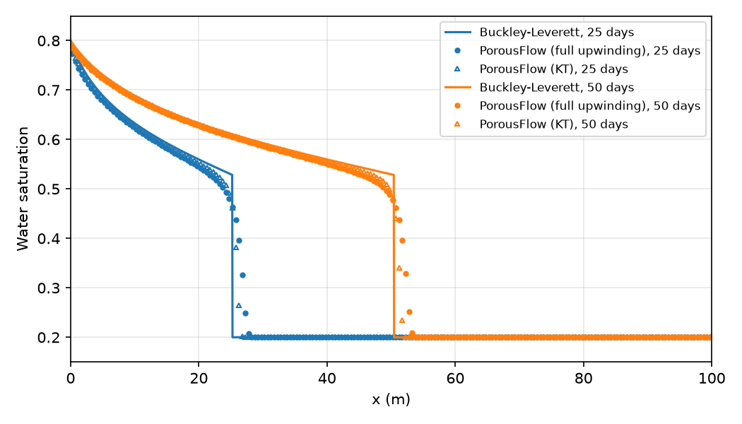
Figure 1: Water saturation in the one-dimensional waterflood after 25 and 50 days: PorousFlow with full upwinding (filled circles) and with Kuzmin-Turek stabilization (open triangles), and the Buckley-Leverett solution (lines).
Both schemes agree with the Buckley-Leverett solution behind the front and place the front correctly (Figure 1). With full upwinding the front is spread over about 34m, slightly ahead of the analytical position, whereas Kuzmin-Turek stabilization resolves it over 12m and comes closer to the saturation at the shock. The front can also be sharpened by refining the mesh. See Numerical stabilization for a discussion of the costs and benefits of each scheme.
Two-dimensional waterflood with wells
The second example is a 200m 200m 10m reservoir with an injection well at and a production well at , using the same fluid and rock properties.
Water is injected at a constant rate of 0.5kgs using a PorousFlowSquarePulsePointSource. An injection PorousFlowPeacemanBorehole is not used here, because the water is immobile at the connate water saturation, so such a well would initially inject nothing.
The production well has a radius of 0.1m and a bottomhole pressure of 19.5MPa. It is represented by one PorousFlowPeacemanBorehole for each phase, so that each phase is produced in proportion to its mobility:
[DiracKernels<<<{"href": "../../syntax/DiracKernels/index.html"}>>>]
  # Water injection at a constant mass rate (kg/s), at mid-thickness of the reservoir
  [injector]
    type = PorousFlowSquarePulsePointSource<<<{"description": "Point source (or sink) that adds (removes) fluid at a constant mass flux rate for times between the specified start and end times.", "href": "../../source/dirackernels/PorousFlowSquarePulsePointSource.html"}>>>
    variable<<<{"description": "The name of the variable that this residual object operates on"}>>> = pwater
    point<<<{"description": "The x,y,z coordinates of the point source (sink)"}>>> = '20 20 5'
    mass_flux<<<{"description": "The mass flux at this point in kg/s (positive is flux in, negative is flux out)"}>>> = 0.5
  []

  # Production well with radius 0.1 m (see producer.bh) and bottomhole pressure 19.5 MPa.
  # For PorousFlowPeacemanBorehole, use_mobility already includes the relative permeability
  [producer_water]
    type = PorousFlowPeacemanBorehole<<<{"description": "Approximates a borehole in the mesh using the Peaceman approach, ie using a number of point sinks with given radii whose positions are read from a file.  NOTE: if you are using PorousFlowPorosity that depends on volumetric strain, you should set strain_at_nearest_qp=true in your GlobalParams, to ensure the nodal Porosity Material uses the volumetric strain at the Dirac quadpoints, and can therefore be computed.  The wellbore pressure profile is built either from a constant fluid unit weight ('unit_weight') or, if a thermal gradient along the borehole makes a single constant unit weight a poor approximation, from a fluid density computed at each borehole point from a temperature-dependent fluid-properties UserObject ('unit_weight_fp')", "href": "../../source/dirackernels/PorousFlowPeacemanBorehole.html"}>>>
    variable<<<{"description": "The name of the variable that this residual object operates on"}>>> = pwater
    SumQuantityUO<<<{"description": "User Object of type=PorousFlowSumQuantity in which to place the total outflow from the line sink for each time step."}>>> = water_produced
    point_file<<<{"description": "The file containing the coordinates of the points and their weightings that approximate the line sink.  The physical meaning of the weightings depend on the scenario, eg, they may be borehole radii.  Each line in the file must contain a space-separated weight and coordinate, viz r x y z.  For boreholes, the last point in the file is defined as the borehole bottom, where the borehole pressure is bottom_pressure.  If your file contains just one point, you must also specify the line_length and line_direction parameters.  Note that you will get segementation faults if your points do not lie within your mesh!"}>>> = producer.bh
    function_of<<<{"description": "Modifying functions will be a function of either pressure and permeability (eg, for boreholes that pump fluids) or temperature and thermal conductivity (eg, for boreholes that pump pure heat with no fluid flow)"}>>> = pressure
    fluid_phase<<<{"description": "The fluid phase whose pressure (and potentially mobility, enthalpy, etc) controls the flux to the line sink.  For p_or_t=temperature, and without any use_*, this parameter is irrelevant"}>>> = 0
    mass_fraction_component<<<{"description": "The index corresponding to a fluid component.  If supplied, the flux will be multiplied by the nodal mass fraction for the component"}>>> = 0
    bottom_p_or_t<<<{"description": "For function_of=pressure, this function is the pressure at the bottom of the borehole, otherwise it is the temperature at the bottom of the borehole."}>>> = 19.5e6
    unit_weight<<<{"description": "(fluid_density*gravitational_acceleration) as a vector pointing downwards.  Note that the borehole pressure at a given z position is bottom_p_or_t + unit_weight*(q - q_bottom), where q=(x,y,z) and q_bottom=(x,y,z) of the bottom point of the borehole.  The analogous formula holds for function_of=temperature.  If you don't want bottomhole pressure (or temperature) to vary in the borehole just set unit_weight=0.  Typical value is = (0,0,-1E4), for water.  Exactly one of 'unit_weight' or 'unit_weight_fp' must be given.  Use 'unit_weight_fp' instead of 'unit_weight' if you want the fluid unit weight to vary along the borehole according to a temperature-dependent fluid density, rather than being a single constant value."}>>> = '0 0 0'
    use_mobility<<<{"description": "Multiply the flux by the fluid mobility"}>>> = true # relative permeability x density / viscosity of the phase
    character<<<{"description": "If zero then borehole does nothing.  If positive the borehole acts as a sink (production well) for porepressure > borehole pressure, and does nothing otherwise.  If negative the borehole acts as a source (injection well) for porepressure < borehole pressure, and does nothing otherwise.  The flow rate to/from the borehole is multiplied by |character|, so usually character = +/- 1, but you can specify other quantities to provide an overall scaling to the flow if you like."}>>> = 1
  []
  [producer_oil]
    type = PorousFlowPeacemanBorehole<<<{"description": "Approximates a borehole in the mesh using the Peaceman approach, ie using a number of point sinks with given radii whose positions are read from a file.  NOTE: if you are using PorousFlowPorosity that depends on volumetric strain, you should set strain_at_nearest_qp=true in your GlobalParams, to ensure the nodal Porosity Material uses the volumetric strain at the Dirac quadpoints, and can therefore be computed.  The wellbore pressure profile is built either from a constant fluid unit weight ('unit_weight') or, if a thermal gradient along the borehole makes a single constant unit weight a poor approximation, from a fluid density computed at each borehole point from a temperature-dependent fluid-properties UserObject ('unit_weight_fp')", "href": "../../source/dirackernels/PorousFlowPeacemanBorehole.html"}>>>
    variable<<<{"description": "The name of the variable that this residual object operates on"}>>> = soil
    SumQuantityUO<<<{"description": "User Object of type=PorousFlowSumQuantity in which to place the total outflow from the line sink for each time step."}>>> = oil_produced
    point_file<<<{"description": "The file containing the coordinates of the points and their weightings that approximate the line sink.  The physical meaning of the weightings depend on the scenario, eg, they may be borehole radii.  Each line in the file must contain a space-separated weight and coordinate, viz r x y z.  For boreholes, the last point in the file is defined as the borehole bottom, where the borehole pressure is bottom_pressure.  If your file contains just one point, you must also specify the line_length and line_direction parameters.  Note that you will get segementation faults if your points do not lie within your mesh!"}>>> = producer.bh
    function_of<<<{"description": "Modifying functions will be a function of either pressure and permeability (eg, for boreholes that pump fluids) or temperature and thermal conductivity (eg, for boreholes that pump pure heat with no fluid flow)"}>>> = pressure
    fluid_phase<<<{"description": "The fluid phase whose pressure (and potentially mobility, enthalpy, etc) controls the flux to the line sink.  For p_or_t=temperature, and without any use_*, this parameter is irrelevant"}>>> = 1
    mass_fraction_component<<<{"description": "The index corresponding to a fluid component.  If supplied, the flux will be multiplied by the nodal mass fraction for the component"}>>> = 1
    bottom_p_or_t<<<{"description": "For function_of=pressure, this function is the pressure at the bottom of the borehole, otherwise it is the temperature at the bottom of the borehole."}>>> = 19.5e6
    unit_weight<<<{"description": "(fluid_density*gravitational_acceleration) as a vector pointing downwards.  Note that the borehole pressure at a given z position is bottom_p_or_t + unit_weight*(q - q_bottom), where q=(x,y,z) and q_bottom=(x,y,z) of the bottom point of the borehole.  The analogous formula holds for function_of=temperature.  If you don't want bottomhole pressure (or temperature) to vary in the borehole just set unit_weight=0.  Typical value is = (0,0,-1E4), for water.  Exactly one of 'unit_weight' or 'unit_weight_fp' must be given.  Use 'unit_weight_fp' instead of 'unit_weight' if you want the fluid unit weight to vary along the borehole according to a temperature-dependent fluid density, rather than being a single constant value."}>>> = '0 0 0'
    use_mobility<<<{"description": "Multiply the flux by the fluid mobility"}>>> = true # relative permeability x density / viscosity of the phase
    character<<<{"description": "If zero then borehole does nothing.  If positive the borehole acts as a sink (production well) for porepressure > borehole pressure, and does nothing otherwise.  If negative the borehole acts as a source (injection well) for porepressure < borehole pressure, and does nothing otherwise.  The flow rate to/from the borehole is multiplied by |character|, so usually character = +/- 1, but you can specify other quantities to provide an overall scaling to the flow if you like."}>>> = 1
  []
[]For PorousFlowPeacemanBorehole, use_mobility = true already includes the relative permeability, so use_relative_permeability should not also be set. This differs from the boundary condition PorousFlowPiecewiseLinearSink used in the one-dimensional example, where the relative permeability is included separately with use_relperm.
The oil and water production rates at surface conditions, the water cut and the cumulative oil production are computed with postprocessors:
[Postprocessors<<<{"href": "../../syntax/Postprocessors/index.html"}>>>]
  [dt]
    type = TimestepSize<<<{"description": "Reports the timestep size", "href": "../../source/postprocessors/TimestepSize.html"}>>>
    outputs<<<{"description": "Vector of output names where you would like to restrict the output of variables(s) associated with this object"}>>> = none
  []
  [water_produced_this_step]
    type = PorousFlowPlotQuantity<<<{"description": "Extracts the value from the PorousFlowSumQuantity UserObject", "href": "../../source/postprocessors/PorousFlowPlotQuantity.html"}>>>
    uo<<<{"description": "PorousFlowSumQuantity user object name that holds the required information"}>>> = water_produced
    outputs<<<{"description": "Vector of output names where you would like to restrict the output of variables(s) associated with this object"}>>> = none
  []
  [oil_produced_this_step]
    type = PorousFlowPlotQuantity<<<{"description": "Extracts the value from the PorousFlowSumQuantity UserObject", "href": "../../source/postprocessors/PorousFlowPlotQuantity.html"}>>>
    uo<<<{"description": "PorousFlowSumQuantity user object name that holds the required information"}>>> = oil_produced
    outputs<<<{"description": "Vector of output names where you would like to restrict the output of variables(s) associated with this object"}>>> = none
  []
  # Production rates at surface conditions (m3/day)
  [oil_rate]
    type = ParsedPostprocessor<<<{"description": "Computes a parsed expression with post-processors", "href": "../../source/postprocessors/ParsedPostprocessor.html"}>>>
    expression<<<{"description": "function expression"}>>> = 'oil / dt / 850 * 86400'
    pp_names<<<{"description": "Post-processors arguments"}>>> = 'oil_produced_this_step dt'
    pp_symbols<<<{"description": "Symbol associated with each post-processor argument"}>>> = 'oil dt'
  []
  [water_rate]
    type = ParsedPostprocessor<<<{"description": "Computes a parsed expression with post-processors", "href": "../../source/postprocessors/ParsedPostprocessor.html"}>>>
    expression<<<{"description": "function expression"}>>> = 'water / dt / 1000 * 86400'
    pp_names<<<{"description": "Post-processors arguments"}>>> = 'water_produced_this_step dt'
    pp_symbols<<<{"description": "Symbol associated with each post-processor argument"}>>> = 'water dt'
  []
  [water_cut]
    type = ParsedPostprocessor<<<{"description": "Computes a parsed expression with post-processors", "href": "../../source/postprocessors/ParsedPostprocessor.html"}>>>
    expression<<<{"description": "function expression"}>>> = 'if(oil + water > 0, water / (oil + water), 0)'
    pp_names<<<{"description": "Post-processors arguments"}>>> = 'oil_rate water_rate'
    pp_symbols<<<{"description": "Symbol associated with each post-processor argument"}>>> = 'oil water'
  []
  # Cumulative production at surface conditions (m3)
  [cumulative_oil]
    type = CumulativeValuePostprocessor<<<{"description": "Creates a cumulative sum of a Postprocessor value with time.", "href": "../../source/postprocessors/CumulativeValuePostprocessor.html"}>>>
    postprocessor<<<{"description": "The name of the postprocessor"}>>> = oil_volume_this_step
  []
  [oil_volume_this_step]
    type = ParsedPostprocessor<<<{"description": "Computes a parsed expression with post-processors", "href": "../../source/postprocessors/ParsedPostprocessor.html"}>>>
    expression<<<{"description": "function expression"}>>> = 'oil / 850'
    pp_names<<<{"description": "Post-processors arguments"}>>> = 'oil_produced_this_step'
    pp_symbols<<<{"description": "Symbol associated with each post-processor argument"}>>> = 'oil'
    outputs<<<{"description": "Vector of output names where you would like to restrict the output of variables(s) associated with this object"}>>> = none
  []
  [p_injector]
    type = PointValue<<<{"description": "Compute the value of a variable at a specified location", "href": "../../source/postprocessors/PointValue.html"}>>>
    variable<<<{"description": "The name of the variable that this postprocessor operates on."}>>> = pwater
    point<<<{"description": "The physical point where the solution will be evaluated."}>>> = '20 20 5'
  []
[]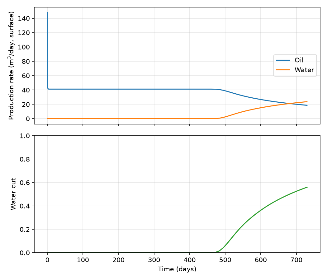
Figure 2: Oil and water production rates at surface conditions (top) and water cut (bottom) for the two-dimensional waterflood.
The production history is shown in Figure 2. After a brief initial period, during which the pressure around the production well falls towards the bottomhole pressure, the oil rate settles at about 41m/day at surface conditions. This corresponds to about 42.6m/day at reservoir conditions (), which balances the injected water volume of about 42.8m/day. Water breaks through at the production well after about 470 days, when about 0.25 pore volumes have been injected. This is less than the 0.42 pore volumes of the one-dimensional case, because the water reaches the production well before it has swept the whole area. After breakthrough the oil rate falls and the water cut rises, reaching about 0.56 after 2 years.
The script plot_waterflood_2d.py in the example directory plots the production history.