The MOOSE Navier-Stokes Module

July 2025

Overview

Main capabilities:

Fluid types:
- Incompressible
- Weakly-compressible
- Compressible
- Two-phase mixture model
Flow regimes:
- Laminar
- Turbulent
Flow types:
- Free flows
- Flows in porous media describing homogenized structures

Utilizes the following techniques:

Stabilized Continuous Finite Element Discretization (maintained, but not intensely developed) (Peterson et al. (2018))
Finite Volume Discretization with nonlinear solver (Lindsay et al. (2023))
Finite Volume Discretization with linear solver

Applicability of each solver

Nonlinear (Newton method) finite volume

2D problems
only solver with support for porous medium
turbulence models (mixing-length, k- $var element = document.getElementById("moose-equation-a63aa46b-de9d-432b-a2af-0420e1e8cc7b");katex.render("\\epsilon", element, {displayMode:false,throwOnError:false,macros:{"\\vec":"\\bar","\\pf":"\\frac{\\partial #1}{\\partial #2}"}});$ )
fully compressible flow problems

Linear (SIMPLE/PIMPLE) finite volume

3D problems

You can check that the combination of models you want is supported in Table 2 on this page The nonlinear (SIMPLE/PIMPLE) finite volume is being replaced by the linear implementation. It is currently still only used for two-phase flow studies.

The Porous Navier-Stokes equations (Vafai (2015), Radman et al. (2021))

Conservation of mass:

(2)var element = document.getElementById("moose-equation-d4bd2976-e61e-4c5e-9084-0ebfefb34024");katex.render("\\frac{\\partial \\gamma \\rho}{\\partial t} + \\nabla \\cdot \\left( \\rho \\vec{u} \\right) = 0", element, {displayMode:true,throwOnError:false,macros:{"\\vec":"\\bar","\\pf":"\\frac{\\partial #1}{\\partial #2}"}});

Conservation of (linear) momentum:

(3)var element = document.getElementById("moose-equation-c6cfaebd-9d76-46e9-ac53-acf55565f23e");katex.render("\\frac{\\partial \\rho \\vec{u}}{\\partial t} + \\nabla \\cdot \\left(\\gamma^{-1} \\rho \\vec{u} \\otimes \\vec{u}\\right) = \\nabla \\cdot \\left(\\gamma \\mu_\\text{eff} \\left(\\nabla\\vec{u}_I + \\left(\\nabla \\vec{u}_I\\right)^T-\\frac{2}{3}\\nabla\\cdot\\vec{u}_I\\mathbb{I}\\right)\\right) -\\gamma\\nabla p + \\gamma \\rho \\vec{g} - W \\vec{u}_I", element, {displayMode:true,throwOnError:false,macros:{"\\vec":"\\bar","\\pf":"\\frac{\\partial #1}{\\partial #2}"}});

$var element = document.getElementById("moose-equation-8c7fc638-05c6-457c-ba7f-55001be1d1d8");katex.render("\\gamma", element, {displayMode:false,throwOnError:false,macros:{"\\vec":"\\bar","\\pf":"\\frac{\\partial #1}{\\partial #2}"}});$ - porosity
$var element = document.getElementById("moose-equation-53029486-890c-4303-bab8-e1d1bdec2479");katex.render("\\vec{u}_I", element, {displayMode:false,throwOnError:false,macros:{"\\vec":"\\bar","\\pf":"\\frac{\\partial #1}{\\partial #2}"}});$ - real (or interstitial) velocity
$var element = document.getElementById("moose-equation-1dc38280-111c-4130-a35c-69c056f0cdf3");katex.render("\\vec{u} \\equiv \\gamma \\vec{u}_I", element, {displayMode:false,throwOnError:false,macros:{"\\vec":"\\bar","\\pf":"\\frac{\\partial #1}{\\partial #2}"}});$ - superficial velocity

$var element = document.getElementById("moose-equation-c990b8d8-cfe7-4bdc-b0e8-210a37c55651");katex.render("\\rho = \\rho(p,T)", element, {displayMode:false,throwOnError:false,macros:{"\\vec":"\\bar","\\pf":"\\frac{\\partial #1}{\\partial #2}"}});$ - density
$var element = document.getElementById("moose-equation-2781f906-9cf1-47ff-8f42-aaaa188d9e11");katex.render("\\mu_{eff}", element, {displayMode:false,throwOnError:false,macros:{"\\vec":"\\bar","\\pf":"\\frac{\\partial #1}{\\partial #2}"}});$ - effective dynamic viscosity (laminar + turbulent)
$var element = document.getElementById("moose-equation-8364592e-8d78-43ff-a542-47ce934e9e4d");katex.render("p", element, {displayMode:false,throwOnError:false,macros:{"\\vec":"\\bar","\\pf":"\\frac{\\partial #1}{\\partial #2}"}});$ - pressure
$var element = document.getElementById("moose-equation-eb28ef12-41aa-4afb-9597-f74762ee202e");katex.render("W", element, {displayMode:false,throwOnError:false,macros:{"\\vec":"\\bar","\\pf":"\\frac{\\partial #1}{\\partial #2}"}});$ - friction tensor (using correlations)

If $var element = document.getElementById("moose-equation-cddb3445-35d6-4cd1-a418-80f3146620a0");katex.render("\\gamma=1", element, {displayMode:false,throwOnError:false,macros:{"\\vec":"\\bar","\\pf":"\\frac{\\partial #1}{\\partial #2}"}});$ then $var element = document.getElementById("moose-equation-2343f569-f05b-4700-ba5b-a150f71d4e38");katex.render("\\vec{u}=\\vec{u}_I", element, {displayMode:false,throwOnError:false,macros:{"\\vec":"\\bar","\\pf":"\\frac{\\partial #1}{\\partial #2}"}});$ and we get the original Navier-Stokes equations back.

The Porous Navier-Stokes equations (contd.)

These are supplemented by the conservation of energy:
Assumptions: Weakly-compressible fluid, kinetic energy of the fluid can be neglected

(1)var element = document.getElementById("moose-equation-287933da-b243-48bd-9ba4-8328d92fa66c");katex.render("\\frac{\\partial \\gamma \\rho c_p T}{\\partial t} + \\nabla \\cdot \\left( \\rho c_p T \\vec{u}\\right) = \\nabla \\cdot \\left(\\kappa_f \\nabla T \\right) - \\alpha (T - T_s) + S_{ext}", element, {displayMode:true,throwOnError:false,macros:{"\\vec":"\\bar","\\pf":"\\frac{\\partial #1}{\\partial #2}"}});

$var element = document.getElementById("moose-equation-0a85154c-3c6a-4976-aebc-4d8f7dd9ac22");katex.render("c_p", element, {displayMode:false,throwOnError:false,macros:{"\\vec":"\\bar","\\pf":"\\frac{\\partial #1}{\\partial #2}"}});$ - specific heat
$var element = document.getElementById("moose-equation-68e33264-dd51-4357-8c92-d92716dc90b1");katex.render("T", element, {displayMode:false,throwOnError:false,macros:{"\\vec":"\\bar","\\pf":"\\frac{\\partial #1}{\\partial #2}"}});$ - fluid temperature
$var element = document.getElementById("moose-equation-0e558456-4f9d-4714-8e6a-9c7c78d09634");katex.render("\\kappa_f", element, {displayMode:false,throwOnError:false,macros:{"\\vec":"\\bar","\\pf":"\\frac{\\partial #1}{\\partial #2}"}});$ - effective thermal conductivity

$var element = document.getElementById("moose-equation-b14cba93-8295-4c49-b753-1c6ec40bf7fd");katex.render("\\alpha", element, {displayMode:false,throwOnError:false,macros:{"\\vec":"\\bar","\\pf":"\\frac{\\partial #1}{\\partial #2}"}});$ - volumetric heat-transfer coefficient (using correlations)
$var element = document.getElementById("moose-equation-4fe0e40b-6a6f-4c5b-861c-bfe83e994113");katex.render("T_s", element, {displayMode:false,throwOnError:false,macros:{"\\vec":"\\bar","\\pf":"\\frac{\\partial #1}{\\partial #2}"}});$ - solid temperature
$var element = document.getElementById("moose-equation-27a017a1-13bc-4995-bfcf-69b569ea4b22");katex.render("S_{ext}", element, {displayMode:false,throwOnError:false,macros:{"\\vec":"\\bar","\\pf":"\\frac{\\partial #1}{\\partial #2}"}});$ - volumetric source term

The Porous Navier-Stokes equations (contd.)

The equations are extended with initial and boundary conditions:

Few examples:
- Velocity Inlet: $var element = document.getElementById("moose-equation-ece91d24-4ff1-44ad-860f-c23c3f93314a");katex.render("\\vec{u}=\\vec{u}_{inlet}, \\quad T=T_{inlet}, \\quad \\vec{r} \\in \\partial\\Omega_{inlet}", element, {displayMode:false,throwOnError:false,macros:{"\\vec":"\\bar","\\pf":"\\frac{\\partial #1}{\\partial #2}"}});$
- Pressure Outlet: $var element = document.getElementById("moose-equation-e838eb78-e09a-4887-82f6-cdb347bb135f");katex.render("p = p_{outlet}, \\quad \\vec{r} \\in \\partial\\Omega_{outlet}", element, {displayMode:false,throwOnError:false,macros:{"\\vec":"\\bar","\\pf":"\\frac{\\partial #1}{\\partial #2}"}});$
- No-slip, insulated walls: $var element = document.getElementById("moose-equation-57144f59-6329-40d2-ab6f-dd317abefa1e");katex.render("\\vec{u}=\\vec{0}, \\quad \\kappa_f \\nabla T \\cdot \\vec{n} = 0, \\quad \\vec{r} \\in \\partial\\Omega_{wall}", element, {displayMode:false,throwOnError:false,macros:{"\\vec":"\\bar","\\pf":"\\frac{\\partial #1}{\\partial #2}"}});$
- Heat flux on the walls: $var element = document.getElementById("moose-equation-719d4912-b753-4b87-bb10-91a36c1ae653");katex.render("\\quad -\\kappa_f \\nabla T \\big|_{\\partial \\Omega} \\cdot \\vec{n} = q^{\\prime \\prime}, \\quad \\vec{r} \\in \\partial\\Omega_{heated}", element, {displayMode:false,throwOnError:false,macros:{"\\vec":"\\bar","\\pf":"\\frac{\\partial #1}{\\partial #2}"}});$
- Free slip on walls: $var element = document.getElementById("moose-equation-6661c53b-6165-498b-aaf2-321e5321fd00");katex.render("\\vec{u} \\cdot \\vec{n} = 0, \\quad \\vec{r} \\in \\partial\\Omega_{slip}", element, {displayMode:false,throwOnError:false,macros:{"\\vec":"\\bar","\\pf":"\\frac{\\partial #1}{\\partial #2}"}});$
- ...

Useful Acronyms

Good to know before navigating source code and documentation:

NS - Navier-Stokes
FV - Finite Volume
I - Incompressible
WC - Weakly-Compressible
C - Compressible
P - Porous-Medium

Few Examples:

PINSFV: Porous-Medium Incompressible Navier-Stokes Finite Volume
WCNSFV: Weakly-Compressible Navier-Stokes Finite Volume
WCNSLinearFV: Weakly-Compressible Navier-Stokes Linear Finite Volume

Building Input Files

The building blocks in MOOSE for terms in the PDEs are Kernels for FE, FVKernels for FV, and LinearFVKernels for SIMPLE-FV:

var element = document.getElementById("moose-equation-3a381561-c6db-4f6f-a0e8-a58c42f7633c");katex.render("\\underbrace{\\frac{\\partial \\rho \\vec{u}}{\\partial t}}_{\\text{PINSFVMomentumTimeDerivative}} + \\underbrace{\\nabla \\cdot \\left(\\gamma^{-1} \\rho \\vec{u} \\otimes \\vec{u}\\right)}_{\\text{PINSFVMomentumAdvection}} =", element, {displayMode:true,throwOnError:false,macros:{"\\vec":"\\bar","\\pf":"\\frac{\\partial #1}{\\partial #2}"}});

var element = document.getElementById("moose-equation-988da6a5-f9c4-48d3-878f-e7b798bc6d15");katex.render("\\underbrace{\\nabla \\cdot \\left(\\gamma \\mu_\\text{eff} \\left(\\nabla\\vec{u}_I + \\left(\\nabla \\vec{u}_I\\right)^T-\\frac{2}{3}\\nabla\\cdot\\vec{u}_I\\mathbb{I}\\right)\\right)}_{\\text{PINSFVMomentumDiffusion}} \\underbrace{-\\gamma\\nabla p}_{\\text{PINSFVMomentumPressure}} + \\underbrace{\\gamma\\rho \\vec{g}}_{\\text{PINSFVMomentumGravity~}} \\underbrace{- W \\vec{u}_I}_{\\text{PINSFVMomentumFriction}}", element, {displayMode:true,throwOnError:false,macros:{"\\vec":"\\bar","\\pf":"\\frac{\\partial #1}{\\partial #2}"}});

The building blocks in MOOSE for boundary conditions are BCs for FE, FVBCs for Newton-FV, and LinearFVBCs for SIMPLE-FV:

Inlet Velocity: $var element = document.getElementById("moose-equation-580ff505-9cba-4a48-83df-d1f07b9f5258");katex.render("\\text{INSFVInletVelocityBC}", element, {displayMode:false,throwOnError:false,macros:{"\\vec":"\\bar","\\pf":"\\frac{\\partial #1}{\\partial #2}"}});$
Inlet Temperature: $var element = document.getElementById("moose-equation-ff24cf46-d242-4253-9610-4891b986ddbe");katex.render("\\text{FVFunctionDirichletBC}", element, {displayMode:false,throwOnError:false,macros:{"\\vec":"\\bar","\\pf":"\\frac{\\partial #1}{\\partial #2}"}});$
Outlet pressure: $var element = document.getElementById("moose-equation-7218d3f1-d8c5-4c82-992a-c1fb140912da");katex.render("\\text{INSFVOutletPressureBC}", element, {displayMode:false,throwOnError:false,macros:{"\\vec":"\\bar","\\pf":"\\frac{\\partial #1}{\\partial #2}"}});$
Heatflux: $var element = document.getElementById("moose-equation-10006c8a-1108-41da-8cf5-15e70e16d67a");katex.render("\\text{FVFunctionNeumannBC}", element, {displayMode:false,throwOnError:false,macros:{"\\vec":"\\bar","\\pf":"\\frac{\\partial #1}{\\partial #2}"}});$
Freeslip: $var element = document.getElementById("moose-equation-0b47fa11-efd1-49a2-aeb0-f438a44079a6");katex.render("\\text{INSFVNaturalFreeSlipBC}", element, {displayMode:false,throwOnError:false,macros:{"\\vec":"\\bar","\\pf":"\\frac{\\partial #1}{\\partial #2}"}});$
...

A Simple Example: Laminar Free Flow in a Channel

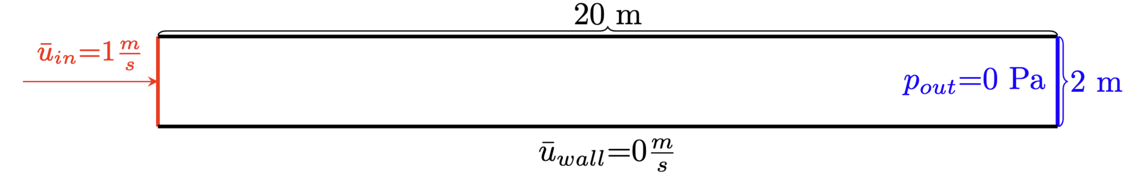
Let us consider the following (fictional) material properties:

$var element = document.getElementById("moose-equation-ea361073-6941-4dd8-b017-76170b3d4fdd");katex.render("\\mu=1.1", element, {displayMode:false,throwOnError:false,macros:{"\\vec":"\\bar","\\pf":"\\frac{\\partial #1}{\\partial #2}"}});$ $var element = document.getElementById("moose-equation-ed60e9d8-5217-4c77-ad62-08e325509897");katex.render("\\text{Pa}\\cdot\\text{s}", element, {displayMode:false,throwOnError:false,macros:{"\\vec":"\\bar","\\pf":"\\frac{\\partial #1}{\\partial #2}"}});$
$var element = document.getElementById("moose-equation-8a6ca87f-052c-42f8-b2b1-5615005a0c35");katex.render("\\rho=1.1", element, {displayMode:false,throwOnError:false,macros:{"\\vec":"\\bar","\\pf":"\\frac{\\partial #1}{\\partial #2}"}});$ $var element = document.getElementById("moose-equation-77ca1c98-8710-46da-b692-3e9654c56d4c");katex.render("\\frac{kg}{m^3}", element, {displayMode:false,throwOnError:false,macros:{"\\vec":"\\bar","\\pf":"\\frac{\\partial #1}{\\partial #2}"}});$ (we are using incompressible formulation in this case)

Detailed Input File (nonlinear/Newton FV)

mu = 1.1
rho = 1.1
l = 2
U = 1
advected_interp_method = 'average'
velocity_interp_method = 'rc'

[GlobalParams]
  rhie_chow_user_object = 'rc'
[]

[UserObjects]
  [rc]
    type = INSFVRhieChowInterpolator
    u = vel_x
    v = vel_y
    pressure = pressure
  []
[]

[Mesh]
  [gen]
    type = GeneratedMeshGenerator
    dim = 2
    xmin = 0
    xmax = 10
    ymin = ${fparse -l / 2}
    ymax = ${fparse l / 2}
    nx = 100
    ny = 20
  []
  uniform_refine = 0
[]

[Variables]
  [vel_x]
    type = INSFVVelocityVariable
    initial_condition = 1
  []
  [vel_y]
    type = INSFVVelocityVariable
    initial_condition = 1
  []
  [pressure]
    type = INSFVPressureVariable
  []
[]

[FVKernels]
  [mass]
    type = INSFVMassAdvection
    variable = pressure
    advected_interp_method = ${advected_interp_method}
    velocity_interp_method = ${velocity_interp_method}
    rho = ${rho}
  []

  [u_advection]
    type = INSFVMomentumAdvection
    variable = vel_x
    advected_interp_method = ${advected_interp_method}
    velocity_interp_method = ${velocity_interp_method}
    rho = ${rho}
    momentum_component = 'x'
  []
  [u_viscosity]
    type = INSFVMomentumDiffusion
    variable = vel_x
    mu = ${mu}
    momentum_component = 'x'
  []
  [u_pressure]
    type = INSFVMomentumPressure
    variable = vel_x
    momentum_component = 'x'
    pressure = pressure
  []

  [v_advection]
    type = INSFVMomentumAdvection
    variable = vel_y
    advected_interp_method = ${advected_interp_method}
    velocity_interp_method = ${velocity_interp_method}
    rho = ${rho}
    momentum_component = 'y'
  []
  [v_viscosity]
    type = INSFVMomentumDiffusion
    variable = vel_y
    mu = ${mu}
    momentum_component = 'y'
  []
  [v_pressure]
    type = INSFVMomentumPressure
    variable = vel_y
    momentum_component = 'y'
    pressure = pressure
  []
[]

[FVBCs]
  [inlet-u]
    type = INSFVInletVelocityBC
    boundary = 'left'
    variable = vel_x
    function = '${U}'
  []
  [inlet-v]
    type = INSFVInletVelocityBC
    boundary = 'left'
    variable = vel_y
    function = '0'
  []
  [walls-u]
    type = INSFVNoSlipWallBC
    boundary = 'top bottom'
    variable = vel_x
    function = 0
  []
  [walls-v]
    type = INSFVNoSlipWallBC
    boundary = 'top bottom'
    variable = vel_y
    function = 0
  []
  [outlet_p]
    type = INSFVOutletPressureBC
    boundary = 'right'
    variable = pressure
    function = '0'
  []
[]

[Executioner]
  type = Steady
  solve_type = 'NEWTON'
  nl_rel_tol = 1e-12
[]

[Preconditioning]
  active = FSP
  [FSP]
    type = FSP
    # It is the starting point of splitting
    topsplit = 'up' # 'up' should match the following block name
    [up]
      splitting = 'u p' # 'u' and 'p' are the names of subsolvers
      splitting_type  = schur
      # Splitting type is set as schur, because the pressure part of Stokes-like systems
      # is not diagonally dominant. CAN NOT use additive, multiplicative and etc.
      #
      # Original system:
      #
      # | Auu Aup | | u | = | f_u |
      # | Apu 0   | | p |   | f_p |
      #
      # is factorized into
      #
      # |I             0 | | Auu  0|  | I  Auu^{-1}*Aup | | u | = | f_u |
      # |Apu*Auu^{-1}  I | | 0   -S|  | 0  I            | | p |   | f_p |
      #
      # where
      #
      # S = Apu*Auu^{-1}*Aup
      #
      # The preconditioning is accomplished via the following steps
      #
      # (1) p* = f_p - Apu*Auu^{-1}f_u,
      # (2) p = (-S)^{-1} p*
      # (3) u = Auu^{-1}(f_u-Aup*p)

      petsc_options_iname = '-pc_fieldsplit_schur_fact_type  -pc_fieldsplit_schur_precondition -ksp_gmres_restart -ksp_rtol -ksp_type'
      petsc_options_value = 'full                            selfp                             300                1e-4      fgmres'
    []
    [u]
      vars = 'vel_x vel_y'
      petsc_options_iname = '-pc_type -pc_hypre_type -ksp_type -ksp_rtol -ksp_gmres_restart -ksp_pc_side'
      petsc_options_value = 'hypre    boomeramg      gmres    5e-1      300                 right'
    []
    [p]
      vars = 'pressure'
      petsc_options_iname = '-ksp_type -ksp_gmres_restart -ksp_rtol -pc_type -ksp_pc_side'
      petsc_options_value = 'gmres    300                5e-1      jacobi    right'
    []
  []
  [SMP]
    type = SMP
    full = true
    petsc_options_iname = '-pc_type -pc_factor_shift_type'
    petsc_options_value = 'lu       NONZERO'
  []
[]

[Outputs]
  print_linear_residuals = true
  print_nonlinear_residuals = true
  [out]
    type = Exodus
    hide = 'Re lin cum_lin'
  []
  [perf]
    type = PerfGraphOutput
  []
[]

[Postprocessors]
  [Re]
    type = ParsedPostprocessor
    expression = '${rho} * ${l} * ${U}'
  []
  [lin]
    type = NumLinearIterations
  []
  [cum_lin]
    type = CumulativeValuePostprocessor
    postprocessor = lin
  []
[]

(modules/navier_stokes/test/tests/finite_volume/ins/channel-flow/2d-rc-no-slip.i)

Detailed Input File (linear/SIMPLE FV)

mu = 2.6
rho = 1.0
advected_interp_method = 'average'

[Mesh]
  [mesh]
    type = CartesianMeshGenerator
    dim = 2
    dx = '0.3'
    dy = '0.3'
    ix = '3'
    iy = '3'
  []
[]

[Problem]
  linear_sys_names = 'u_system v_system pressure_system'
  previous_nl_solution_required = true
[]

[UserObjects]
  [rc]
    type = RhieChowMassFlux
    u = vel_x
    v = vel_y
    pressure = pressure
    rho = ${rho}
    p_diffusion_kernel = p_diffusion
  []
[]

[Variables]
  [vel_x]
    type = MooseLinearVariableFVReal
    initial_condition = 0.5
    solver_sys = u_system
  []
  [vel_y]
    type = MooseLinearVariableFVReal
    solver_sys = v_system
    initial_condition = 0.0
  []
  [pressure]
    type = MooseLinearVariableFVReal
    solver_sys = pressure_system
    initial_condition = 0.2
  []
[]

[LinearFVKernels]
  [u_advection_stress]
    type = LinearWCNSFVMomentumFlux
    variable = vel_x
    advected_interp_method = ${advected_interp_method}
    mu = ${mu}
    u = vel_x
    v = vel_y
    momentum_component = 'x'
    rhie_chow_user_object = 'rc'
    use_nonorthogonal_correction = false
  []
  [v_advection_stress]
    type = LinearWCNSFVMomentumFlux
    variable = vel_y
    advected_interp_method = ${advected_interp_method}
    mu = ${mu}
    u = vel_x
    v = vel_y
    momentum_component = 'y'
    rhie_chow_user_object = 'rc'
    use_nonorthogonal_correction = false
  []
  [u_pressure]
    type = LinearFVMomentumPressure
    variable = vel_x
    pressure = pressure
    momentum_component = 'x'
  []
  [v_pressure]
    type = LinearFVMomentumPressure
    variable = vel_y
    pressure = pressure
    momentum_component = 'y'
  []
  [p_diffusion]
    type = LinearFVAnisotropicDiffusion
    variable = pressure
    diffusion_tensor = Ainv
    use_nonorthogonal_correction = false
  []
  [HbyA_divergence]
    type = LinearFVDivergence
    variable = pressure
    face_flux = HbyA
    force_boundary_execution = true
  []
[]

[LinearFVBCs]
  [inlet-u]
    type = LinearFVAdvectionDiffusionFunctorDirichletBC
    boundary = 'left'
    variable = vel_x
    functor = '1.1'
  []
  [inlet-v]
    type = LinearFVAdvectionDiffusionFunctorDirichletBC
    boundary = 'left'
    variable = vel_y
    functor = '0.0'
  []
  [walls-u]
    type = LinearFVAdvectionDiffusionFunctorDirichletBC
    boundary = 'top bottom'
    variable = vel_x
    functor = 0.0
  []
  [walls-v]
    type = LinearFVAdvectionDiffusionFunctorDirichletBC
    boundary = 'top bottom'
    variable = vel_y
    functor = 0.0
  []
  [outlet_p]
    type = LinearFVAdvectionDiffusionFunctorDirichletBC
    boundary = 'right'
    variable = pressure
    functor = 1.4
  []
  [outlet_u]
    type = LinearFVAdvectionDiffusionOutflowBC
    variable = vel_x
    use_two_term_expansion = false
    boundary = right
  []
  [outlet_v]
    type = LinearFVAdvectionDiffusionOutflowBC
    variable = vel_y
    use_two_term_expansion = false
    boundary = right
  []
[]

[Executioner]
  type = SIMPLE
  momentum_l_abs_tol = 1e-10
  pressure_l_abs_tol = 1e-10
  momentum_l_tol = 0
  pressure_l_tol = 0
  rhie_chow_user_object = 'rc'
  momentum_systems = 'u_system v_system'
  pressure_system = 'pressure_system'
  momentum_equation_relaxation = 0.8
  pressure_variable_relaxation = 0.3
  num_iterations = 100
  pressure_absolute_tolerance = 1e-10
  momentum_absolute_tolerance = 1e-10
  momentum_petsc_options_iname = '-pc_type -pc_hypre_type'
  momentum_petsc_options_value = 'hypre boomeramg'
  pressure_petsc_options_iname = '-pc_type -pc_hypre_type'
  pressure_petsc_options_value = 'hypre boomeramg'
  print_fields = false
[]

[Outputs]
  exodus = true
[]

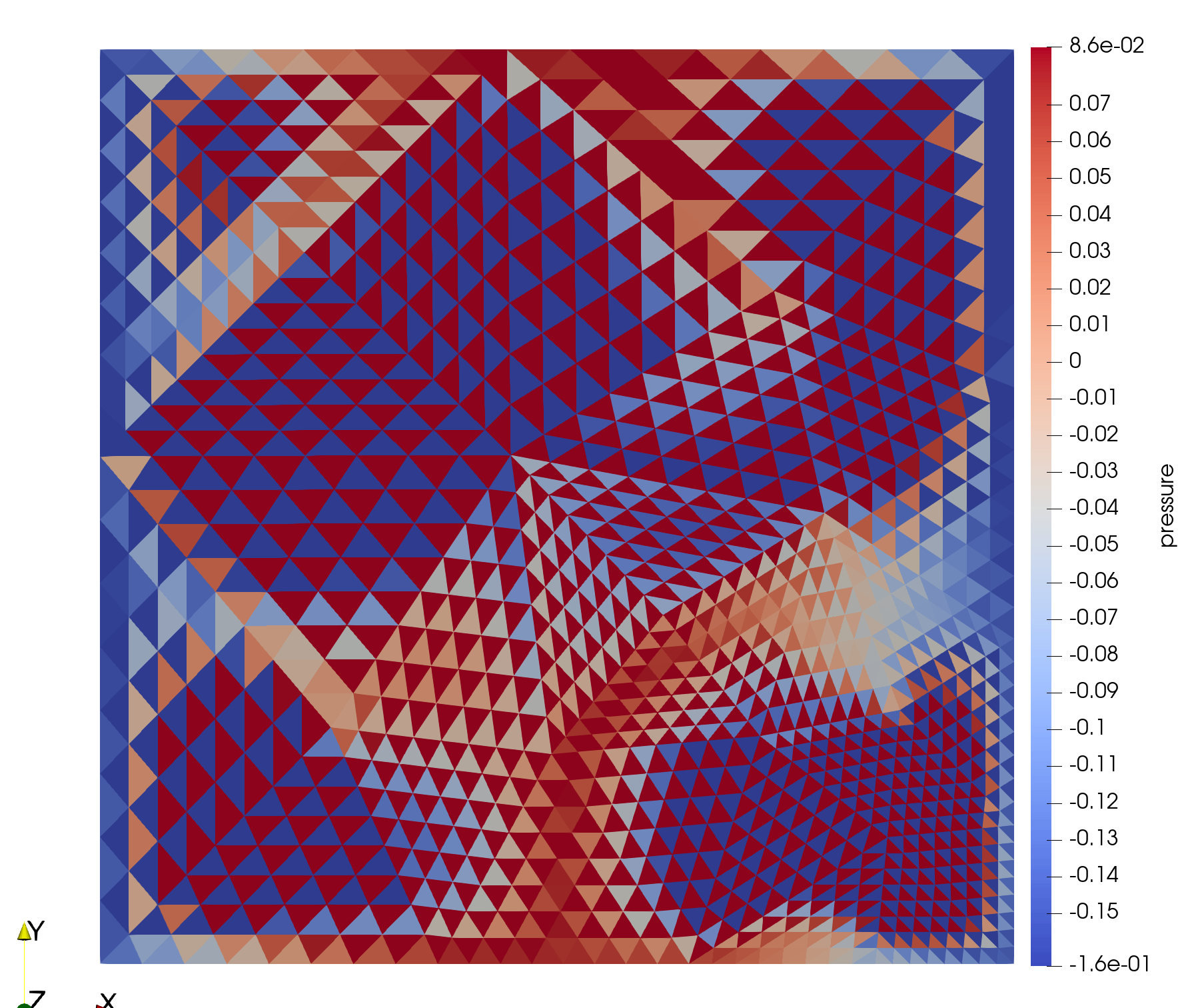
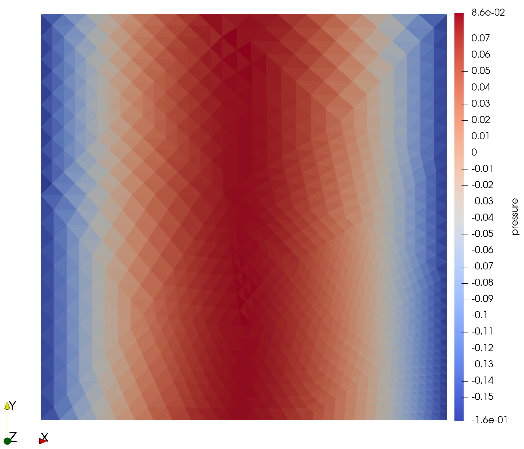
(modules/navier_stokes/test/tests/finite_volume/ins/channel-flow/linear-segregated/2d/2d-velocity-pressure.i)

Rhie-Chow Interpolation

When using linear interpolation for the advecting velocity and the pressure gradient, we encounter a checker-boarding effect for the pressure field. Neighboring cell center solution values are decoupled, which is undesirable.
Solution for this issue: Rhie-Chow interpolation for the advecting velocity. For more information on the issue and the derivation of the interpolation method, see Moukalled et al. (2016).

$var element = document.getElementById("moose-equation-57ae0907-e8f5-4fab-b0ea-169d63f85e57");katex.render("\\Large\\xrightarrow[\\mathrm{Rhie-Chow~Interpolation}]{\\vec{u}_{RC,f} = \\vec{u}_{AVG,f} - \\left(\\frac{1}{a}\\right)_f\\left(\\nabla p_f - \\overline{\\nabla p}_f\\right)}", element, {displayMode:false,throwOnError:false,macros:{"\\vec":"\\bar","\\pf":"\\frac{\\partial #1}{\\partial #2}"}});$

The Navier-Stokes Physics

A simplified syntax has been developed, it relies on the Physics system in MOOSE. Each Physics is in charge of creating one equation. The input below shows the flow and energy conservation equations. Only the finite volume discretization, for the Newton and PIMPLE solvers, support this syntax.

mu = 1
rho = 1
k = 1e-3
cp = 1
u_inlet = 1
T_inlet = 200
h_cv = 1.0

[Mesh]
  [mesh]
    type = CartesianMeshGenerator
    dim = 2
    dx = '5 5'
    dy = '1.0'
    ix = '50 50'
    iy = '20'
    subdomain_id = '1 2'
  []
[]

[Variables]
  [T_solid]
    type = MooseVariableFVReal
  []
[]

[AuxVariables]
  [porosity]
    type = MooseVariableFVReal
    initial_condition = 0.5
  []
[]

[Physics]
  [NavierStokes]
    [Flow]
      [flow]
        compressibility = 'incompressible'
        porous_medium_treatment = true

        density = ${rho}
        dynamic_viscosity = ${mu}
        porosity = 'porosity'

        initial_velocity = '${u_inlet} 1e-6 0'
        initial_pressure = 0.0

        inlet_boundaries = 'left'
        momentum_inlet_types = 'fixed-velocity'
        momentum_inlet_function = '${u_inlet} 0'

        wall_boundaries = 'top bottom'
        momentum_wall_types = 'noslip symmetry'

        outlet_boundaries = 'right'
        momentum_outlet_types = 'fixed-pressure'
        pressure_function = '0.1'

        mass_advection_interpolation = 'average'
        momentum_advection_interpolation = 'average'
      []
    []
    [FluidHeatTransfer]
      [heat]
        thermal_conductivity = ${k}
        specific_heat = ${cp}

        # Reference file sets effective_conductivity by default that way
        # so the conductivity is multiplied by the porosity in the kernel
        effective_conductivity = false

        initial_temperature = 0.0

        energy_inlet_types = 'heatflux'
        energy_inlet_function = '${fparse u_inlet * rho * cp * T_inlet}'

        energy_wall_types = 'heatflux heatflux'
        energy_wall_function = '0 0'

        ambient_convection_alpha = ${h_cv}
        ambient_temperature = 'T_solid'

        energy_advection_interpolation = 'average'
      []
    []
  []
[]

[FVKernels]
  [solid_energy_diffusion]
    type = FVDiffusion
    coeff = ${k}
    variable = T_solid
  []
  [solid_energy_convection]
    type = PINSFVEnergyAmbientConvection
    variable = 'T_solid'
    is_solid = true
    T_fluid = 'T_fluid'
    T_solid = 'T_solid'
    h_solid_fluid = ${h_cv}
  []
[]

[FVBCs]
  [heated-side]
    type = FVDirichletBC
    boundary = 'top'
    variable = 'T_solid'
    value = 150
  []
[]

[Executioner]
  type = Steady
  solve_type = 'NEWTON'
  petsc_options_iname = '-pc_type -pc_factor_shift_type'
  petsc_options_value = 'lu NONZERO'
  nl_rel_tol = 1e-14
[]

# Some basic Postprocessors to examine the solution
[Postprocessors]
  [inlet-p]
    type = SideAverageValue
    variable = pressure
    boundary = 'left'
  []
  [outlet-u]
    type = SideAverageValue
    variable = superficial_vel_x
    boundary = 'right'
  []
  [outlet-temp]
    type = SideAverageValue
    variable = T_fluid
    boundary = 'right'
  []
  [solid-temp]
    type = ElementAverageValue
    variable = T_solid
  []
[]

[Outputs]
  exodus = true
  csv = false
[]

(modules/navier_stokes/test/tests/finite_volume/pins/channel-flow/heated/2d-rc-heated-physics.i)

Recommendations for Building Input Files

Check that the combination of models you want is supported in Table 2 there
Start from an example. If no example, find a test that looks similar.
If possible, use the Navier Stokes finite volume Physics syntax
Use Rhie-Chow interpolation for the advecting velocity
- Other interpolation techniques may lead to checkerboarding/instability

Start with first-order advected-interpolation schemes (e.g. upwind)
Make sure that the pressure is pinned for incompressible/weakly-compressible simulations in closed systems
For monolithic solvers (the default at the moment) use a variant of LU preconditioner
For complex monolithic systems monitor the residuals of every variable
Try to keep the number of elements relatively low (limited scaling with LU preconditioner $var element = document.getElementById("moose-equation-ae7a2644-3bc0-4003-a6e3-e928bf3b35b5");katex.render("^*", element, {displayMode:false,throwOnError:false,macros:{"\\vec":"\\bar","\\pf":"\\frac{\\partial #1}{\\partial #2}"}});$ ). Larger problems can be solved in a reasonable wall-time as segregated-solve techniques are introduced
Try to utilize porosity_smoothing_layers or a higher value for the consistent_scaling if you encounter oscillatory behavior in case of simulations using porous medium

$var element = document.getElementById("moose-equation-45328bd6-79c4-4571-90b2-612de2f97aa9");katex.render("^*", element, {displayMode:false,throwOnError:false,macros:{"\\vec":"\\bar","\\pf":"\\frac{\\partial #1}{\\partial #2}"}});$ Because the complexity of the LU preconditioner is $var element = document.getElementById("moose-equation-37311aa9-8625-4922-841d-7fd91cada5b7");katex.render("N^3", element, {displayMode:false,throwOnError:false,macros:{"\\vec":"\\bar","\\pf":"\\frac{\\partial #1}{\\partial #2}"}});$ in the worst case scenario, its performance in general largely depends on the matrix sparsity pattern, and it is much more expensive compared with an iterative approach.

Validation studies and additional examples

Turbulence modeling for Molten Salt Reactors

Open-Pronghorn flow test bed (to be released soon)

References

Alexander Lindsay, Guillaume Giudicelli, Peter German, John Peterson, Yaqi Wang, Ramiro Freile, David Andrs, Paolo Balestra, Mauricio Tano, Rui Hu, and others. Moose navier–stokes module. SoftwareX, 23:101503, 2023.
Fadl Moukalled, L Mangani, Marwan Darwish, and others. The finite volume method in computational fluid dynamics. Volume 6. Springer, 2016.
John W. Peterson, Alexander D. Lindsay, and Fande Kong. Overview of the incompressible navier–stokes simulation capabilities in the moose framework. Advances in Engineering Software, 119:68–92, 2018.
Stefan Radman, Carlo Fiorina, and Andreas Pautz. Development of a novel two-phase flow solver for nuclear reactor analysis: algorithms, verification and implementation in openfoam. Nuclear Engineering and Design, 379:111178, 2021.
Kambiz Vafai. Handbook of porous media. Crc Press, 2015.