Natural Convection
Problem statement
This example is based on the Elder problem Elder (1967), see Oldenburg et al. (1995). The natural convection of water in a 2D porous tank heated on one part of the bottom is modelled. The schematic is demonstrated in Figure 1. The experiment details are elaborated in the referred paper so will not be shown here to avoid repetition. The governing equations and associated Kernels that describe this problem are provided in detail here.
Table 1: Parameters of the problem (Oldenburg et al., 1995).
| Symbol | Quantity | Value | Units |
|---|---|---|---|
| Porosity | |||
| Permeability | |||
| Viscosity () | |||
| Thermal conductivity | |||
| Heat capacity of rock | || | ||
| Gravity | |||
| Initial temperature |
.](../../media/porous_flow/Convec_schematic.png)
Figure 1: The experiment schematic (Oldenburg et al., 1995).
Input file setup
This section describes the input file syntax.
Mesh
The first step is to set up the mesh. In this problem, a rectangular tank with a width of 300 m and a height of 150 m is simulated. For convenience, instead of the YZ coordinate as shown in Figure 1, the simulation was set up in XY coordinate with the positive Y direction pointing toward the top of the tank. In this code block, the numbers of nodes in the X and Y directions are specified along with the dimension of the tank. A notable feature is the declaration of the boundary heater. This is due to the fact that the heat element at the bottom of the tank is located between 0< x < 150 m. This enables simple boundary condition implementation at later stages.
[Mesh<<<{"href": "../../syntax/Mesh/index.html"}>>>]
  [gen]
    type = GeneratedMeshGenerator<<<{"description": "Create a line, square, or cube mesh with uniformly spaced or biased elements.", "href": "../../source/meshgenerators/GeneratedMeshGenerator.html"}>>>
    dim<<<{"description": "The dimension of the mesh to be generated"}>>> = 2
    nx<<<{"description": "Number of elements in the X direction"}>>> = 64
    ny<<<{"description": "Number of elements in the Y direction"}>>> = 32
    xmin<<<{"description": "Lower X Coordinate of the generated mesh"}>>> = 0
    xmax<<<{"description": "Upper X Coordinate of the generated mesh"}>>> = 300
    ymax<<<{"description": "Upper Y Coordinate of the generated mesh"}>>> = 0
    ymin<<<{"description": "Lower Y Coordinate of the generated mesh"}>>> = -150
  []
  [heater]
    type = ParsedGenerateSideset<<<{"description": "A MeshGenerator that adds element sides to a sideset if the centroid of the side satisfies the `combinatorial_geometry` expression.", "href": "../../source/meshgenerators/ParsedGenerateSideset.html"}>>>
    input<<<{"description": "The mesh we want to modify"}>>> = gen
    combinatorial_geometry<<<{"description": "Function expression encoding a combinatorial geometry"}>>> = 'x <= 150 & y = -150'
    new_sideset_name<<<{"description": "The name of the new sideset"}>>> = heater
  []
  uniform_refine<<<{"description": "Specify the level of uniform refinement applied to the initial mesh"}>>> = 1
[]Fluid properties
After the mesh has been specified, we need to provide the fluid properties that are used for this simulation. For our case, it will be just water and can be easily implemented as follows:
[FluidProperties<<<{"href": "../../syntax/FluidProperties/index.html"}>>>]
  [water]
    type = Water97FluidProperties<<<{"description": "Fluid properties for water and steam (H2O) using IAPWS-IF97", "href": "../../source/fluidproperties/Water97FluidProperties.html"}>>>
  []
[]Variables declaration
Since we are focusing on the natural convection of flow in a porous medium, temperature (T) and porepressure are used.
[Variables<<<{"href": "../../syntax/Variables/index.html"}>>>]
  [porepressure]
  []
  [T]
    initial_condition<<<{"description": "Specifies a constant initial condition for this variable"}>>> = 285
  []
[]Action declaration
For this problem, we use the PorousFlowFullySaturated to automatically add all of the physics kernels and a number of the necessary material properties. As this is a TH problem, we set coupling_type = Thermohydro.
[PorousFlowFullySaturated<<<{"href": "../../syntax/PorousFlowFullySaturated/index.html"}>>>]
  coupling_type<<<{"description": "The type of simulation.  For simulations involving Mechanical deformations, you will need to supply the correct Biot coefficient.  For simulations involving Thermal flows, you will need an associated ConstantThermalExpansionCoefficient Material"}>>> = ThermoHydro
  porepressure<<<{"description": "The name of the porepressure variable"}>>> = porepressure
  temperature<<<{"description": "For isothermal simulations, this is the temperature at which fluid properties (and stress-free strains) are evaluated at.  Otherwise, this is the name of the temperature variable.  Units = Kelvin"}>>> = T
  fp<<<{"description": "The name of the user object for fluid properties. Only needed if fluid_properties_type = PorousFlowSingleComponentFluid"}>>> = water
[]Additional material properties not added by the action are specified in the Materials block.
[Materials<<<{"href": "../../syntax/Materials/index.html"}>>>]
  [porosity]
    type = PorousFlowPorosityConst<<<{"description": "This Material calculates the porosity assuming it is constant", "href": "../../source/materials/PorousFlowPorosityConst.html"}>>>
    porosity<<<{"description": "The porosity (assumed indepenent of porepressure, temperature, strain, etc, for this material).  This should be a real number, or a constant monomial variable (not a linear lagrange or other kind of variable)."}>>> = 0.1
  []
  [permeability]
    type = PorousFlowPermeabilityConst<<<{"description": "This Material calculates the permeability tensor assuming it is constant", "href": "../../source/materials/PorousFlowPermeabilityConst.html"}>>>
    permeability<<<{"description": "The permeability tensor (usually in m^2), which is assumed constant for this material"}>>> = '1.21E-10 0 0   0 1.21E-10 0   0 0 1.21E-10'
  []
  [Matrix_internal_energy]
    type = PorousFlowMatrixInternalEnergy<<<{"description": "This Material calculates the internal energy of solid rock grains, which is specific_heat_capacity * density * temperature.  Kernels multiply this by (1 - porosity) to find the energy density of the porous rock in a rock-fluid system", "href": "../../source/materials/PorousFlowMatrixInternalEnergy.html"}>>>
    density<<<{"description": "Density of the rock grains"}>>> = 2500
    specific_heat_capacity<<<{"description": "Specific heat capacity of the rock grains (J/kg/K)."}>>> = 0
  []
  [thermal_conductivity]
    type = PorousFlowThermalConductivityIdeal<<<{"description": "This Material calculates rock-fluid combined thermal conductivity by using a weighted sum.  Thermal conductivity = dry_thermal_conductivity + S^exponent * (wet_thermal_conductivity - dry_thermal_conductivity), where S is the aqueous saturation", "href": "../../source/materials/PorousFlowThermalConductivityIdeal.html"}>>>
    dry_thermal_conductivity<<<{"description": "The thermal conductivity of the rock matrix when the aqueous saturation is zero"}>>> = '1.5 0 0  0 1.5 0  0 0 0'
  []
[]Initial and Boundary Conditions
The next step is to supply the initial and boundary conditions. For this problem, two initial conditions need to be implemented. The first one is a constant temperature of 285 K which was declared in the previous section. The second one is the hydrostatic variation of porepressure along the y direction as shown below:
[ICs<<<{"href": "../../syntax/ICs/index.html"}>>>]
  [hydrostatic]
    type = FunctionIC<<<{"description": "An initial condition that uses a normal function of x, y, z to produce values (and optionally gradients) for a field variable.", "href": "../../source/ics/FunctionIC.html"}>>>
    variable<<<{"description": "The variable this initial condition is supposed to provide values for."}>>> = porepressure
    function<<<{"description": "The initial condition function."}>>> = '1e5 - 9.81 * 1000 * y'
  []
[]Shifting to the boundary conditions. There are three Dirichlet boundary conditions that we need to supply. The first two are constant temperature at the top and heater surfaces denoted as t_top and t_bot. And, the last one is constant pressure at the top surface denoted as p_top.
[BCs<<<{"href": "../../syntax/BCs/index.html"}>>>]
  [t_bot]
    type = DirichletBC<<<{"description": "Imposes the essential boundary condition $u=g$, where $g$ is a constant, controllable value.", "href": "../../source/bcs/DirichletBC.html"}>>>
    variable<<<{"description": "The name of the variable that this residual object operates on"}>>> = T
    value<<<{"description": "Value of the BC"}>>> = 293
    boundary<<<{"description": "The list of boundary IDs from the mesh where this object applies"}>>> = 'heater'
  []
  [t_top]
    type = DirichletBC<<<{"description": "Imposes the essential boundary condition $u=g$, where $g$ is a constant, controllable value.", "href": "../../source/bcs/DirichletBC.html"}>>>
    variable<<<{"description": "The name of the variable that this residual object operates on"}>>> = T
    value<<<{"description": "Value of the BC"}>>> = 285
    boundary<<<{"description": "The list of boundary IDs from the mesh where this object applies"}>>> = 'top'
  []
  [p_top]
    type = DirichletBC<<<{"description": "Imposes the essential boundary condition $u=g$, where $g$ is a constant, controllable value.", "href": "../../source/bcs/DirichletBC.html"}>>>
    variable<<<{"description": "The name of the variable that this residual object operates on"}>>> = porepressure
    value<<<{"description": "Value of the BC"}>>> = 1e5
    boundary<<<{"description": "The list of boundary IDs from the mesh where this object applies"}>>> = top
  []
[]Executioner setup
Lastly, we will tell Moose the type of the problem (shown in the code block below). For this problem, a transient solver is required. To save time and computational resources, IterationAdaptiveDT and mesh Adaptivity were implemented. The former enables the time step to be increased if the solution converges and decreased if it does not. This will help save time if a large time step can be used and aid in convergence if a small time step is required. Similarly, the latter enables the mesh to automatically adapt to optimize the computational resource usage and resolve the area with stiff gradients. The mesh will be coarsened at the regions with low error and refined at the critical areas (high error and stiff gradients). For practice, users can try to disable them by putting the code block into comment and witnessing the difference in the solving time and solution.
[Executioner<<<{"href": "../../syntax/Executioner/index.html"}>>>]
  type = Transient
  end_time = 63072000
  dtmax = 1e6
  nl_rel_tol = 1e-6
  [TimeStepper<<<{"href": "../../syntax/Executioner/TimeStepper/index.html"}>>>]
    type = IterationAdaptiveDT
    dt = 1000
  []
  [Adaptivity<<<{"href": "../../syntax/Executioner/Adaptivity/index.html"}>>>]
    interval<<<{"description": "The number of time steps betweeen each adaptivity phase"}>>> = 1
    refine_fraction<<<{"description": "The fraction of elements or error to refine. Should be between 0 and 1."}>>> = 0.2
    coarsen_fraction<<<{"description": "The fraction of elements or error to coarsen. Should be between 0 and 1."}>>> = 0.3
    max_h_level<<<{"description": "Maximum number of times a single element can be refined. If 0 then infinite."}>>> = 4
  []
[]Auxiliary kernels and variables (optional)
This section is optional since these kernels and variables do not affect the calculation of the desired variable. In this example, we want to output the fluid density at the end of the simulation thus we will add an auxkernel and an auxvariable for it. It can be noticed that the term execute_on = TIMESTEP_END indicates this kernel will be activated to calculate the fluid density at the end of each time step only, thus this calculation does not affect the performance of other tasks.
[AuxVariables<<<{"href": "../../syntax/AuxVariables/index.html"}>>>]
  [density]
    family<<<{"description": "Specifies the family of FE shape functions to use for this variable"}>>> = MONOMIAL
    order<<<{"description": "Specifies the order of the FE shape function to use for this variable (additional orders not listed are allowed)"}>>> = CONSTANT
  []
[][AuxKernels<<<{"href": "../../syntax/AuxKernels/index.html"}>>>]
[density]
type = PorousFlowPropertyAux<<<{"description": "AuxKernel to provide access to properties evaluated at quadpoints. Note that elemental AuxVariables must be used, so that these properties are integrated over each element.", "href": "../../source/auxkernels/PorousFlowPropertyAux.html"}>>>
variable<<<{"description": "The name of the variable that this object applies to"}>>> = density
property<<<{"description": "The fluid property that this auxillary kernel is to calculate"}>>> = density
execute_on<<<{"description": "The list of flag(s) indicating when this object should be executed. For a description of each flag, see https://mooseframework.inl.gov/source/interfaces/SetupInterface.html."}>>> = TIMESTEP_END
[]
[]Result
The input file can be executed and the result is as follows:
Figure 2: Spatial distribution of temperature with a test time of 2 years.
It is obvious that the mesh at the interface between hot and cold fluid is much more refined as discussed while surrounding areas have a coarser mesh.
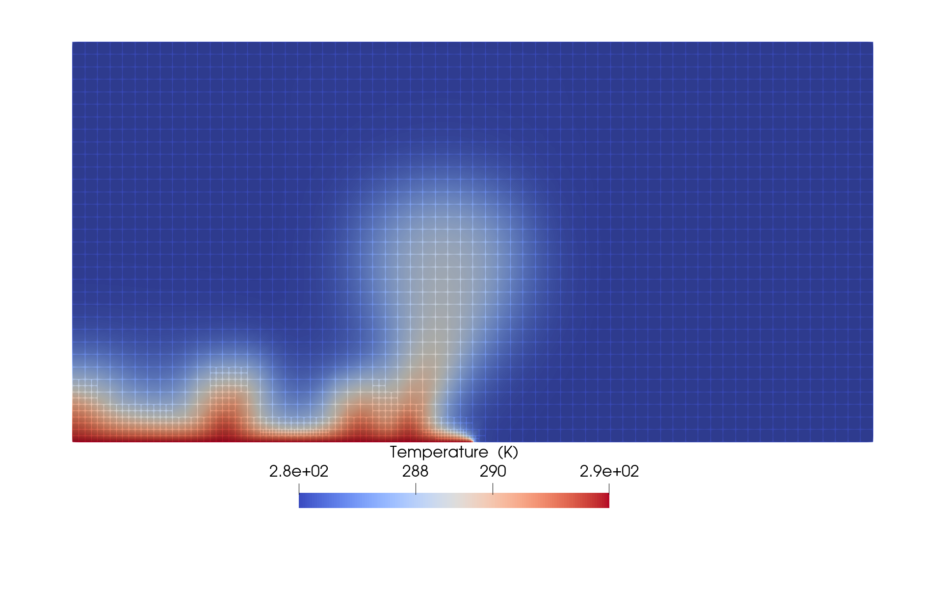
Figure 3: Spatial distribution of temperature at the end of 2 years with mesh grid displayed.
The result from the simulation agrees well with published literature.
.](../../media/porous_flow/Convec_result.png)
Figure 4: Temperature contours and velocity vectors after 2 years (Oldenburg et al., 1995).
References
- Jacob W. Elder.
Transient convection in a porous medium.
Journal of Fluid Mechanics, 27:609 – 623, 1967.
URL: https://api.semanticscholar.org/CorpusID:123656493.[Export]
- C. M. Oldenburg, Ruth L. Hinkins, George J. Moridis, and Karsten Pruess.
On the development of mp-tough2.
Technical Report, Lawrence Berkeley National Laboratory, 1995.
URL: https://api.semanticscholar.org/CorpusID:59668502.[Export]