SCM Tutorial
November 2025
Outline
Introduction to MOOSE
Overview
Key features
Applications
Solving specific physics
SCM Introduction
Motivation
Overview
SCM Model
SCM Model Governing Equations
SCM Model Closure Models
SCM Model Algorithm
Examples
Square lattice geometry
Hexagonal lattice geometry
Introduction to MOOSE
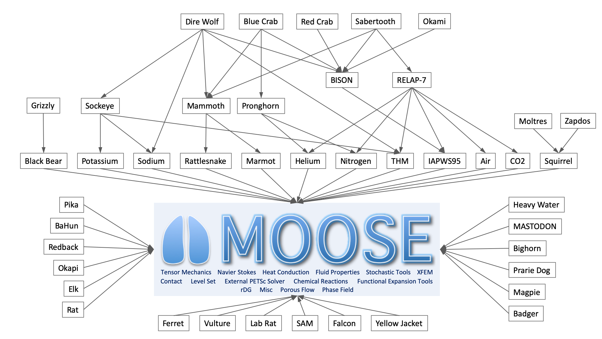
MOOSE Framework: Overview

Developed by Idaho National Laboratory since 2008
Used for studying and analyzing nuclear reactor problems
Free and open source (LGPLv2 license)
Large user community
Highly parallel and HPC capable
Developed and supported by full time INL staff - long-term support
https://www.mooseframework.inl.gov
MOOSE Framework: Key features
Massively parallel computation - successfully run on >100,000 processor cores
Multiphysics solve capability - fully coupled and implicit solver
Multiscale solve capability - multiple application can perform computation for a problem simultaneously
Provides high level interface to implement customized physics, geometries, boundary conditions, and material models
Initially developed to support nuclear R&D but now widely used for non-nuclear R&D also
MOOSE Framework: Applications
MOOSE Framework: Solving specific physics

Custom "kernels" representing specific physics
They can be developed easily and incorporated into the simulation
Introduction to SCM
Motivation
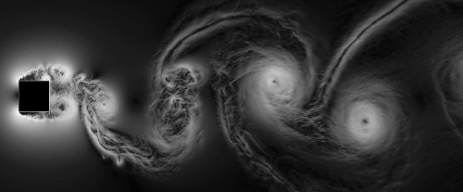
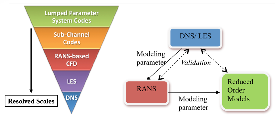
CFD DNS calculations such shown in the left are computationally prohibitive.
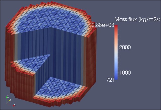
SubChannel calculations such shown in the left (CTF: Isometric view of core mixture mass flux distribution) are practical and fast.
We want to integrate a subchannel code in MOOSE.
This will allow multiphysics and multiscale coupling within MOOSE.
Access numerical solvers supported by PETSc and MOOSE.
Subchannel Overview
The system level thermal hydraulic analysis codes like RELAP, RETRAN, ATHLET are used to get the balance of plant behavior.
The results of this analysis give the boundary conditions used for the core level/component analysis.
The detailed analysis of the reactor core is performed using the subchannel thermal hydraulic codes.
Subchannel codes are thermal-hydraulic codes that offer an efficient compromise for the simulation of a nuclear reactor core, between CFD and system codes
SCM Model
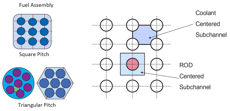
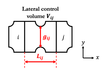
Subchannel discretization principle:
The pin bundle cross section is divided into flow subchannels.
The length of the bundle is divided into finite intervals.
The result is a set of control volumes that represent the flow region of the pin bundle.
Limitations:
Local distributions within a subchannel are not considered. This eliminates the need for zero slip boundary conditions at solid surfaces.
Needs correlations to model wall friction and heat transfer.

SCM Model 2
The governing equations are derived by integrating and averaging the conservation equations (mass, momentum, energy) over the cell volumes
The sub-channel thermal hydraulic analysis solves the conservation equations of mass, momentum and energy on the specified control volumes.
The control volumes are connected in both axial and radial directions.

SCM Model Governing Equations
Mass conservation equation
(1)
Axial momentum conservation equation
(2)
Lateral momentum conservation equation
(3)
Enthalpy conservation equation
(4)
SCM Model Closure Models
Axial direction friction term
Lateral direction friction term
Friction factor
Turbulent momentum diffusion
Turbulent enthalpy diffussion
Turbulent crossflow
SCM Model Algorithm
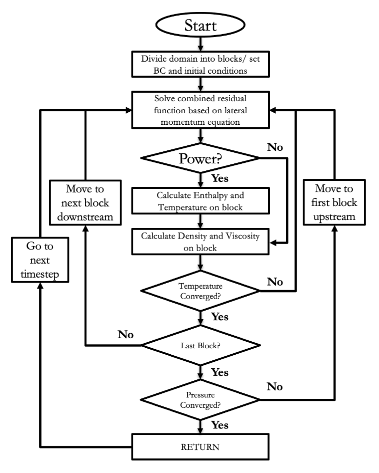
The essense of the algorithm hinges on the construction of a combined residual function based on the lateral momentum equation.
The main unknown variable in this non linear residual is the crossflow . The combined residual function calculates the non linear residual after it updates the other main flow variables.
Once the main flow variables converge in a block, the enthalpy conservation equation is solved. Using enthalpy, pressure and the equations of state, temperature and the fluid properties such as density and viscosity are calculated. After the fluid properties are updated, the solve is repeated until the temperature converges. Once the temperature solution converges the procedure is repeated for the next block downstream until all blocks are solved and pressure converges.
SCM Model Algorithm 2
There are three variations of the algorithm: explicit (default), implicit segregated and implicit monolithic.
Explicit
This is the default algorithm, where the unknown flow variables are calculated in an explicit manner through their governing equations.
Implicit segregated
In this case, the governing equations are recast in matrix form and the flow variables are calculated by solving the corresponding system. Otherwise, the solution algorithm is the same as in the default method.
Implicit monolithic
In this case, the conservation equations are recast in matrix form and combined into a single system. The solution algorithm is the same as in the default method, but the solver used in this version is a fixed point iteration instead of a Newton method. The system looks like this: