Simulating a simple GeoTES experiment
This page describes a reactive-transport simulation of a simple GeoTES scenario. The transport is handled using the PorousFlow module, while the Geochemistry module is used to simulate a heat exchanger and the geochemistry. The simulations are coupled together in an operator-splitting approach using MultiApps.
In Geological Thermal Energy Storage (GeoTES), hot fluid is pumped into an subsurface confined aquifer, stored there for some time, then pumped back again to produce electricity. Many different scenarios have been proposed, including different borehole geometries (used to pump the fluid), different pumping strategies and cyclicities (pumping down certain boreholes, up other boreholes, etc), different temperatures, different aquifer properties, etc. This page only describes the heating phase of a particularly simple set up.
Two wells (boreholes) are used.
The cold (production) well, which pumps aquifer water from the aquifer.
The hot (injection) well, which pumps hot fluid into the aquifer.
These are connected by a heat-exchanger, which heats the aquifer water produced from (1) and passes it to (2). This means the fluid pumped through the injection well is, in fact, heated aquifer water, which is important practically from a water-conservation standpoint, and to assess the geochemical aspects of circulating aquifer water through the GeoTES system.

Figure 1: Schematic of the simple GeoTES simulation.
Aquifer geochemistry
It is assumed that only HO, Na, Cl and SiO(aq) are present in the system. While this is unrealistically simple for any aquifer, it allows this page to focus on the method of constructing more complicated models avoiding rather lengthy input files.
The database file
A small geochemical database involving only these species is used. Readers who are building their own database might find exploring its structure useful:
{
  "Header": {
    "title": "Very small MOOSE thermodynamic database",
    "original": "moose/modules/geochemistry/python/original_dbs/gwb_llnl.dat",
    "date": "09:14 18-08-2020",
    "original format": "gwb",
    "activity model": "debye-huckel",
    "fugacity model": "tsonopoulos",
    "logk model": "fourth-order",
    "logk model (functional form)": "a0 + a1 T + a2 T^2 + a3 T^3 + a4 T^4",
    "temperatures": [
      0.0,
      25.0,
      60.0,
      100.0,
      150.0,
      200.0,
      250.0,
      300.0
    ],
    "pressures": [
      1.0134,
      1.0134,
      1.0134,
      1.0134,
      4.76,
      15.549,
      39.776,
      85.927
    ],
    "adh": [
      0.4913,
      0.5092,
      0.545,
      0.5998,
      0.6898,
      0.8099,
      0.9785,
      1.2555
    ],
    "bdh": [
      0.3247,
      0.3283,
      0.3343,
      0.3422,
      0.3533,
      0.3655,
      0.3792,
      0.3965
    ],
    "bdot": [
      0.0174,
      0.041,
      0.044,
      0.046,
      0.047,
      0.047,
      0.034,
      0.0
    ],
    "neutral species": {
      "co2": {
        "a": [
          0.1224,
          0.1127,
          0.09341,
          0.08018,
          0.08427,
          0.09892,
          0.1371,
          0.1967
        ],
        "b": [
          -0.004679,
          -0.01049,
          -0.0036,
          -0.001503,
          -0.01184,
          -0.0104,
          -0.007086,
          -0.01809
        ],
        "c": [
          -0.0004114,
          0.001545,
          9.609e-05,
          0.0005009,
          0.003118,
          0.001386,
          -0.002887,
          -0.002497
        ],
        "d": [
          0.0,
          0.0,
          0.0,
          0.0,
          0.0,
          0.0,
          0.0,
          0.0
        ]
      },
      "h2o": {
        "a": [
          1.4203,
          1.45397,
          1.5012,
          1.5551,
          1.6225,
          1.6899,
          1.7573,
          1.8247
        ],
        "note": "Missing array values in original database have been filled using a linear fit. Original values are [500.0000, -.0005362, 500.0000, -.0007132, -.0008312, 500.0000, 500.0000, 500.0000]",
        "b": [
          0.0177,
          0.022357,
          0.0289,
          0.036478,
          0.045891,
          0.0553,
          0.0647,
          0.0741
        ],
        "c": [
          0.0103,
          0.0093804,
          0.008,
          0.0064366,
          0.0045221,
          0.0026,
          0.0006,
          -0.0013
        ],
        "d": [
          -0.0005,
          -0.0005362,
          -0.0006,
          -0.0007132,
          -0.0008312,
          -0.0009,
          -0.0011,
          -0.0012
        ]
      }
    }
  },
  "elements": {
    "Cl": {
      "name": "Chlorine",
      "molecular weight": 35.453
    },
    "H": {
      "name": "Hydrogen",
      "molecular weight": 1.0079
    },
    "Na": {
      "name": "Sodium",
      "molecular weight": 22.9898
    },
    "O": {
      "name": "Oxygen",
      "molecular weight": 15.9994
    },
    "Si": {
      "name": "Silicon",
      "molecular weight": 28.085
    }
  },
  "basis species": {
    "H2O": {
      "elements": {
        "H": 2.0,
        "O": 1.0
      },
      "radius": 0.0,
      "charge": 0.0,
      "molecular weight": 18.0152
    },
    "Cl-": {
      "elements": {
        "Cl": 1.0
      },
      "radius": 3.0,
      "charge": -1.0,
      "molecular weight": 35.453
    },
    "Na+": {
      "elements": {
        "Na": 1.0
      },
      "radius": 4.0,
      "charge": 1.0,
      "molecular weight": 22.9898
    },
    "SiO2(aq)": {
      "elements": {
        "O": 2.0,
        "Si": 1.0
      },
      "radius": -0.5,
      "charge": 0.0,
      "molecular weight": 60.0843
    }
  },
  "secondary species": {
    "NaCl": {
      "species": {
        "Na+": 1.0,
        "Cl-": 1.0
      },
      "charge": 0.0,
      "radius": 4.0,
      "molecular weight": 58.4428,
      "logk": [
        1.855,
        1.5994,
        1.2945,
        0.9856,
        0.635,
        0.2935,
        -0.0407,
        -0.3487
      ],
      "note": "Missing array values in original database have been filled using a fourth-order fit. Original values are [1.8550, 1.5994, 1.2945, .9856, .6350, .2935, 500.0000, 500.0000]"
    }
  },
  "free electron": {
    "e-": {
      "species": {
        "H2O": 0.5,
        "O2(g)": -0.25,
        "H+": -1.0
      },
      "charge": -1.0,
      "radius": 0.0,
      "molecular weight": 0.0,
      "logk": [
        22.76135,
        20.7757,
        18.513025,
        16.4658,
        14.473225,
        12.92125,
        11.68165,
        10.67105
      ]
    }
  },
  "mineral species": {
    "QuartzLike": {
      "species": {
        "SiO2(aq)": 1.0
      },
      "molar volume": 22.688,
      "molecular weight": 60.0843,
      "logk": [-5.0, -4.0, -3.0, -2.0, -1.0, 0.0, 1.0, 2.0]
    },
    "QuartzUnlike": {
      "species": {
        "SiO2(aq)": 1.0
      },
      "molar volume": 22.688,
      "molecular weight": 60.0843,
      "logk": [-1.0, -2.0, -3.0, -4.0, -5.0, -6.0, -7.0, -8.0]
    }
  }
}
Initial conditions
The aquifer temperature is uniformly 50C before injection and production.
The aquifer is assumed to be consist entirely of a mineral called QuartzLike and a kinetic rate is used for its dissolution. The mineral QuartzLike is similar to Quartz but it has a different equilibrium constant structure in order to emphasise the dissolution upon heating.
Each 1kg of solvent water is assumed to hold 0.1mol of Na and Cl, and a certain amount of SiO(aq). The following input file finds the free molality of SiO(aq) when in contact with QuartzLike at 50C:
# Finds the equilibrium free molality of SiO2(aq) when in contact with QuartzLike at 50degC
[UserObjects<<<{"href": "../../../syntax/UserObjects/index.html"}>>>]
  [definition]
    type = GeochemicalModelDefinition<<<{"description": "User object that parses a geochemical database file, and only retains information relevant to the current geochemical model", "href": "../../../source/userobjects/GeochemicalModelDefinition.html"}>>>
    database_file<<<{"description": "The name of the geochemical database file"}>>> = "small_database.json"
    basis_species<<<{"description": "A list of basis components relevant to the aqueous-equilibrium problem. H2O must appear first in this list.  These components must be chosen from the 'basis species' in the database, the sorbing sites (if any) and the decoupled redox states that are in disequilibrium (if any)."}>>> = "H2O SiO2(aq) Na+ Cl-"
    equilibrium_minerals<<<{"description": "A list of minerals that are in equilibrium with the aqueous solution.  All members of this list must be in the 'minerals' section of the database file"}>>> = "QuartzLike"
  []
[]

[TimeIndependentReactionSolver<<<{"href": "../../../syntax/TimeIndependentReactionSolver/index.html"}>>>]
  model_definition<<<{"description": "The name of the GeochemicalModelDefinition user object (you must create this UserObject yourself)"}>>> = definition
  geochemistry_reactor_name<<<{"description": "The name that will be given to the GeochemistryReactor UserObject built by this action"}>>> = reactor
  charge_balance_species<<<{"description": "Charge balance will be enforced on this basis species.  This means that its bulk mole number may be changed from the initial value you provide in order to ensure charge neutrality.  After the initial swaps have been performed, this must be in the basis, and it must be provided with a bulk_composition constraint_meaning."}>>> = "Cl-"
  swap_out_of_basis<<<{"description": "Species that should be removed from the model_definition's basis and be replaced with the swap_into_basis species"}>>> = "SiO2(aq)"
  swap_into_basis<<<{"description": "Species that should be removed from the model_definition's equilibrium species list and added to the basis.  There must be the same number of species in swap_out_of_basis and swap_into_basis.  These swaps are performed before any other computations during the initial problem setup. If this list contains more than one species, the swapping is performed one-by-one, starting with the first pair (swap_out_of_basis[0] and swap_into_basis[0]), then the next pair, etc"}>>> = QuartzLike
  constraint_species<<<{"description": "Names of the species that have their values fixed to constraint_value with meaning constraint_meaning.  All basis species (after swap_into_basis and swap_out_of_basis) must be provided with exactly one constraint.  These constraints are used to compute the configuration during the initial problem setup, and in time-dependent simulations they may be modified as time progresses."}>>> = "H2O              Na+              Cl-              QuartzLike"
  constraint_value<<<{"description": "Numerical value of the containts on constraint_species"}>>> = "  1.0              0.1              0.1              396.685" # amount of QuartzLike is unimportant (provided it is positive).  396.685 is used simply because the other geotes_2D input files use this amount
  constraint_meaning<<<{"description": "Meanings of the numerical values given in constraint_value.  kg_solvent_water: can only be applied to H2O and units must be kg.  bulk_composition: can be applied to all non-gas species, and represents the total amount of the basis species contained as free species as well as the amount found in secondary species but not in kinetic species, and units must be moles or mass (kg, g, etc).  bulk_composition_with_kinetic: can be applied to all non-gas species, and represents the total amount of the basis species contained as free species as well as the amount found in secondary species and in kinetic species, and units must be moles or mass (kg, g, etc).  free_concentration: can be applied to all basis species that are not gas and not H2O and not mineral, and represents the total amount of the basis species existing freely (not as secondary species) within the solution, and units must be molal or mass_per_kg_solvent.  free_mineral: can be applied to all mineral basis species, and represents the total amount of the mineral existing freely (precipitated) within the solution, and units must be moles, mass or cm3.  activity and log10activity: can be applied to basis species that are not gas and not mineral and not sorbing sites, and represents the activity of the basis species (recall pH = -log10activity), and units must be dimensionless.  fugacity and log10fugacity: can be applied to gases, and units must be dimensionless"}>>> = "kg_solvent_water bulk_composition bulk_composition free_mineral"
  constraint_unit<<<{"description": "Units of the numerical values given in constraint_value.  Dimensionless: should only be used for activity or fugacity constraints.  Moles: mole number.  Molal: moles per kg solvent water.  kg: kilograms.  g: grams.  mg: milligrams.  ug: micrograms.  kg_per_kg_solvent: kilograms per kg solvent water.  g_per_kg_solvent: grams per kg solvent water.  mg_per_kg_solvent: milligrams per kg solvent water.  ug_per_kg_solvent: micrograms per kg solvent water.  cm3: cubic centimeters"}>>> = "   kg               moles            moles            moles"
  temperature<<<{"description": "The temperature (degC) of the aqueous solution"}>>> = 50.0
  ramp_max_ionic_strength_initial<<<{"description": "The number of iterations over which to progressively increase the maximum ionic strength (from zero to max_ionic_strength) during the initial equilibration.  Increasing this can help in convergence of the Newton process, at the cost of spending more time finding the aqueous configuration."}>>> = 0 # max_ionic_strength in such a simple problem does not need ramping
  add_aux_pH<<<{"description": "Add AuxVariable, called pH, that records the pH of solvent water"}>>> = false # there is no H+ in this system
  precision<<<{"description": "Precision for printing values"}>>> = 12
[]

[Postprocessors<<<{"href": "../../../syntax/Postprocessors/index.html"}>>>]
  [free_moles_SiO2]
    type = PointValue<<<{"description": "Compute the value of a variable at a specified location", "href": "../../../source/postprocessors/PointValue.html"}>>>
    point<<<{"description": "The physical point where the solution will be evaluated."}>>> = '0 0 0'
    variable<<<{"description": "The name of the variable that this postprocessor operates on."}>>> = 'molal_SiO2(aq)'
  []
[]

[Outputs<<<{"href": "../../../syntax/Outputs/index.html"}>>>]
  csv<<<{"description": "Output the scalar variable and postprocessors to a *.csv file using the default CSV output."}>>> = true
[]The result it molality = 0.000555052386. It is necessary to find this initial molality, only because QuartzLike is a kinetic species, so cannot appear the basis (see another similar example). If it were treated as an equilibrium species, its initial free mole number could be specified in the input file below (see an example of this).
Spatially-dependent geochemistry simulation
Because an operator-splitting approach is used, the simulation of the aquifer geochemistry may be considered separately from the porous-flow simulation and the heat exchanger simulation. This section describes how the aquifer geochemistry is simulated.
The model set-up commences with defining the basis species, minerals, and the rate description for the kinetic dissolution of QuartzLike:
[UserObjects<<<{"href": "../../../syntax/UserObjects/index.html"}>>>]
  [rate_quartz]
    type = GeochemistryKineticRate<<<{"description": "User object that defines a kinetic rate.  Note that more than one rate can be prescribed to a single kinetic_species: the sum the individual rates defines the overall rate.  GeochemistryKineticRate simply specifies the algebraic form for a kinetic rate: to actually use it in a calculation, you must use it in the GeochemicalModelDefinition.  The rate is intrinsic_rate_constant * area_quantity * (optionally, mass of kinetic_species in grams) * kinetic_molality^kinetic_molal_index / (kinetic_molality^kinetic_molal_index + kinetic_half_saturation^kinetic_molal_index)^kinetic_monod_index * (product_over_promoting_species m^promoting_index / (m^promoting_index + promoting_half_saturation^promiting_index)^promoting_monod_index) * |1 - (Q/K)^theta|^eta * exp(activation_energy / R * (1/T0 - 1/T)) * Direction(1 - (Q/K)).  Please see the markdown documentation for examples", "href": "../../../source/userobjects/GeochemistryKineticRate.html"}>>>
    kinetic_species_name<<<{"description": "The name of the kinetic species that will be controlled by this rate"}>>> = QuartzLike
    intrinsic_rate_constant<<<{"description": "The intrinsic rate constant for the reaction"}>>> = 1.0E-2
    multiply_by_mass<<<{"description": "Whether the rate should be multiplied by the kinetic_species mass (in grams)"}>>> = true
    area_quantity<<<{"description": "The surface area of the kinetic species in m^2 (if multiply_by_mass = false) or the specific surface area of the kinetic species in m^2/g (if multiply_by_mass = true)"}>>> = 1
    activation_energy<<<{"description": "Activation energy, in J.mol^-1, which appears in exp(activation_energy / R * (1/T0 - 1/T))"}>>> = 72800.0
  []
  [definition]
    type = GeochemicalModelDefinition<<<{"description": "User object that parses a geochemical database file, and only retains information relevant to the current geochemical model", "href": "../../../source/userobjects/GeochemicalModelDefinition.html"}>>>
    database_file<<<{"description": "The name of the geochemical database file"}>>> = "small_database.json"
    basis_species<<<{"description": "A list of basis components relevant to the aqueous-equilibrium problem. H2O must appear first in this list.  These components must be chosen from the 'basis species' in the database, the sorbing sites (if any) and the decoupled redox states that are in disequilibrium (if any)."}>>> = "H2O SiO2(aq) Na+ Cl-"
    kinetic_minerals<<<{"description": "A list of minerals whose dynamics are governed by a rate law.  These are not in equilibrium with the aqueous solution.  All members of this list must be in the 'minerals' section of the database file."}>>> = "QuartzLike"
    kinetic_rate_descriptions<<<{"description": "A list of GeochemistryKineticRate UserObject names that define the kinetic rates.  If a kinetic species has no rate prescribed to it, its reaction rate will be zero"}>>> = "rate_quartz"
  []
  [nodal_void_volume_uo]
    type = NodalVoidVolume<<<{"description": "UserObject to compute the nodal void volume.  Take care if you block-restrict this UserObject, since the volumes of the nodes on the block's boundary will not include any contributions from outside the block.", "href": "../../../source/userobjects/NodalVoidVolume.html"}>>>
    porosity<<<{"description": "Porosity"}>>> = porosity
    execute_on<<<{"description": "The list of flag(s) indicating when this object should be executed. For a description of each flag, see https://mooseframework.inl.gov/source/interfaces/SetupInterface.html."}>>> = 'initial timestep_end' # "initial" means this is evaluated properly for the first timestep
  []
[]The parameters in the rate description are similar to those chosen in another example.
A SpatialReactionSolver defines the initial concentrations of the species and how reactants are added to the system
[SpatialReactionSolver<<<{"href": "../../../syntax/SpatialReactionSolver/index.html"}>>>]
  model_definition<<<{"description": "The name of the GeochemicalModelDefinition user object (you must create this UserObject yourself)"}>>> = definition
  geochemistry_reactor_name<<<{"description": "The name that will be given to the GeochemistryReactor UserObject built by this action"}>>> = reactor
  charge_balance_species<<<{"description": "Charge balance will be enforced on this basis species.  This means that its bulk mole number may be changed from the initial value you provide in order to ensure charge neutrality.  After the initial swaps have been performed, this must be in the basis, and it must be provided with a bulk_composition constraint_meaning."}>>> = "Cl-"
  constraint_species<<<{"description": "Names of the species that have their values fixed to constraint_value with meaning constraint_meaning.  All basis species (after swap_into_basis and swap_out_of_basis) must be provided with exactly one constraint.  These constraints are used to compute the configuration during the initial problem setup, and in time-dependent simulations they may be modified as time progresses."}>>> = "H2O              Na+              Cl-              SiO2(aq)"
  # ASSUME that 1 litre of solution contains:
  constraint_value<<<{"description": "Numerical value of the containts on constraint_species"}>>> = "  1.0              0.1              0.1              0.000555052386"
  constraint_meaning<<<{"description": "Meanings of the numerical values given in constraint_value.  kg_solvent_water: can only be applied to H2O and units must be kg.  bulk_composition: can be applied to all non-gas species, and represents the total amount of the basis species contained as free species as well as the amount found in secondary species but not in kinetic species, and units must be moles or mass (kg, g, etc).  bulk_composition_with_kinetic: can be applied to all non-gas species, and represents the total amount of the basis species contained as free species as well as the amount found in secondary species and in kinetic species, and units must be moles or mass (kg, g, etc).  free_concentration: can be applied to all basis species that are not gas and not H2O and not mineral, and represents the total amount of the basis species existing freely (not as secondary species) within the solution, and units must be molal or mass_per_kg_solvent.  free_mineral: can be applied to all mineral basis species, and represents the total amount of the mineral existing freely (precipitated) within the solution, and units must be moles, mass or cm3.  activity and log10activity: can be applied to basis species that are not gas and not mineral and not sorbing sites, and represents the activity of the basis species (recall pH = -log10activity), and units must be dimensionless.  fugacity and log10fugacity: can be applied to gases, and units must be dimensionless"}>>> = "kg_solvent_water bulk_composition bulk_composition free_concentration"
  constraint_unit<<<{"description": "Units of the numerical values given in constraint_value.  Dimensionless: should only be used for activity or fugacity constraints.  Moles: mole number.  Molal: moles per kg solvent water.  kg: kilograms.  g: grams.  mg: milligrams.  ug: micrograms.  kg_per_kg_solvent: kilograms per kg solvent water.  g_per_kg_solvent: grams per kg solvent water.  mg_per_kg_solvent: milligrams per kg solvent water.  ug_per_kg_solvent: micrograms per kg solvent water.  cm3: cubic centimeters"}>>> = "   kg               moles            moles            molal"
  initial_temperature<<<{"description": "Temperature at which the initial system is equilibrated.  This is uniform over the entire mesh."}>>> = 50.0
  kinetic_species_name<<<{"description": "Names of the kinetic species given initial values in kinetic_species_initial_value"}>>> = QuartzLike
  # Per 1 litre (1000cm^3) of aqueous solution (1kg of solvent water), there is 9000cm^3 of QuartzLike, which means the initial porosity is 0.1.
  kinetic_species_initial_value<<<{"description": "Initial number of moles, mass or volume (depending on kinetic_species_unit) for each of the species named in kinetic_species_name"}>>> = 9000
  kinetic_species_unit<<<{"description": "Units of the numerical values given in kinetic_species_initial_value.  Moles: mole number.  kg: kilograms.  g: grams.  mg: milligrams.  ug: micrograms.  cm3: cubic centimeters"}>>> = cm3
  temperature<<<{"description": "Temperature"}>>> = temperature
  source_species_names<<<{"description": "The name of the species that are added at rates given in source_species_rates.  There must be an equal number of these as source_species_rates."}>>> = 'H2O    Na+   Cl-   SiO2(aq)'
  source_species_rates<<<{"description": "Rates, in mols/time_unit, of addition of the species with names given in source_species_names.  A negative value corresponds to removing a species: be careful that you don't cause negative mass problems!"}>>> = 'rate_H2O_per_1l rate_Na_per_1l rate_Cl_per_1l rate_SiO2_per_1l'
  ramp_max_ionic_strength_initial<<<{"description": "The number of iterations over which to progressively increase the maximum ionic strength (from zero to max_ionic_strength) during the initial equilibration.  Increasing this can help in convergence of the Newton process, at the cost of spending more time finding the aqueous configuration."}>>> = 0 # max_ionic_strength in such a simple problem does not need ramping
  add_aux_pH<<<{"description": "Add AuxVariable, called pH, that records the pH of solvent water"}>>> = false # there is no H+ in this system
  evaluate_kinetic_rates_always<<<{"description": "If true, then, evaluate the kinetic rates at every Newton step during the solve using the current values of molality, activity, etc (ie, implement an implicit solve).  If false, then evaluate the kinetic rates using the values of molality, activity, etc, at the start of the current time step (ie, implement an explicit solve)"}>>> = true # implicit time-marching used for stability
  execute_console_output_on<<<{"description": "When to execute the geochemistry console output"}>>> = ''
[]Most lines in this block need further discussion.
Since this is a
SpatialReactionSolver, the system described exists at each node in the mesh. Each node will typically have a different void volume fraction associated to it: nodes in coarsely-meshed regions will be responsible for large volumes of fluid, while nodes in finely-meshed regions, or regions with small porosity, will represent small volumes of fluid. In the above setup, just 1 liter of aqueous solution is modelled at each node. As discussed below, the rates of reactant additions will be adjusted to reflect this. It is assumed that 1 liter of aqueous solution contains 1.0kg of solvent water and the specified quantities of Na, Cl and SiO(aq).The
free_molalityconstraint on SiO(aq) is set according to the equilibrium simulation described above.It is assumed that there is 9000cm of
QuartzLikeper the 1000cm (1 liter) of aqueous solution. This corresponds to 396.685mol ofQuartzLike. The reason for choosing 9000cm ofQuartzLikeis that the aquifer porosity is assumed to be 0.1 and to be calculated using:
The initial
temperatureof the aquifer is assumed to be 50C, and during simulation it is given by theAuxVariablecalledtemperature. ThisAuxVariablewill be provided by the PorousFlow simulation described below.The
source_species_ratesare defined by therate_*_per_1lAuxVariableswhich are discussed further below.
The Mesh and Executioner are provided in the input file so that it may be run alone in a stand-alone fashion, but these are overwritten when coupled with the PorousFlow simulation (below). The remainder of the input file deals with AuxVariables that are used to transfer information to-and-from the PorousFlow simulation.
The PorousFlow simulation provides temperature, pf_rate_H2O, pf_rate_Na, pf_rate_Cl and pf_rate_SiO2 as AuxVariables. The pf_rate quantities are rates of changes of fluid-component mass (kg.s) at each node, but the Geochemistry module expects rates-of-changes of moles (mol.s) at each node. Moreover, since this input file considers just 1 liter of aqueous solution at every node, the nodal_void_volume is used to convert to mol.s/(liter of aqueous solution). For instance:
  [rate_H2O_per_1l_auxk]
    type = ParsedAux
    coupled_variables = 'pf_rate_H2O nodal_void_volume'
    variable = rate_H2O_per_1l
# pf_rate = change in kg at every node
# pf_rate * 1000 / molar_mass_in_g_per_mole = change in moles at every node
# pf_rate * 1000 / molar_mass / (nodal_void_volume_in_m^3 * 1000) = change in moles per litre of aqueous solution
    expression = 'pf_rate_H2O / 18.0152 / nodal_void_volume'
    execute_on = 'timestep_begin'
[]This input file provides the PorousFlow simulation with updated mass-fractions (after QuartzLike dissolution has occurred to increase the SiO(aq) concentration, for instance). These are based on the "transported" mole numbers at each node, which are the mole numbers of the transported species in the original basis (mole numbers of HO, Na, Cl and free moles of SiO(aq) in this case). These are recorded into AuxVariables using, for example:
  [transported_H2O_auxk]
    type = GeochemistryQuantityAux
    variable = transported_H2O
    species = H2O
    quantity = transported_moles_in_original_basis
    execute_on = 'timestep_end'
[]The mass fraction is computed using, for example
  [transported_mass_auxk]
    type = ParsedAux
    coupled_variables = 'transported_H2O transported_Na transported_Cl transported_SiO2'
    variable = transported_mass
    expression = 'transported_H2O * 18.0152 + transported_Na * 22.9898 + transported_Cl * 35.453 + transported_SiO2 * 60.0843'
    execute_on = 'timestep_end'
  []
  [massfrac_H2O]
    type = ParsedAux
    coupled_variables = 'transported_H2O transported_mass'
    variable = massfrac_H2O
    expression = 'transported_H2O * 18.0152 / transported_mass'
    execute_on = 'timestep_end'
[]The PorousFlow simulation
The PorousFlow module is used to perform the transport. It is assumed the aquifer may be adequately modelled using a 2D mesh. The injection well is at and the production well at :
[Mesh<<<{"href": "../../../syntax/Mesh/index.html"}>>>]
  [gen]
    type = GeneratedMeshGenerator<<<{"description": "Create a line, square, or cube mesh with uniformly spaced or biased elements.", "href": "../../../source/meshgenerators/GeneratedMeshGenerator.html"}>>>
    dim<<<{"description": "The dimension of the mesh to be generated"}>>> = 2
    nx<<<{"description": "Number of elements in the X direction"}>>> = 14 # for better resolution, use 56 or 112
    ny<<<{"description": "Number of elements in the Y direction"}>>> = 8 # for better resolution, use 32 or 64
    xmin<<<{"description": "Lower X Coordinate of the generated mesh"}>>> = -70
    xmax<<<{"description": "Upper X Coordinate of the generated mesh"}>>> = 70
    ymin<<<{"description": "Lower Y Coordinate of the generated mesh"}>>> = -40
    ymax<<<{"description": "Upper Y Coordinate of the generated mesh"}>>> = 40
  []
  [injection_node]
    input<<<{"description": "The mesh we want to modify"}>>> = gen
    type = ExtraNodesetGenerator<<<{"description": "Creates a new node set and a new boundary made with the nodes the user provides.", "href": "../../../source/meshgenerators/ExtraNodesetGenerator.html"}>>>
    new_boundary<<<{"description": "The names of the boundaries to create"}>>> = injection_node
    coord<<<{"description": "The nodes with coordinates you want to be in the nodeset. Separate multple coords with ';' (Either this parameter or \"nodes\" must be supplied)."}>>> = '-30 0 0'
  []
[]1.0 30 0 0
Recall that the PorousFlow module considers mass fractions, not mole-fractions or molalities, etc. Denoting the mass-fraction of Na by f0, the mass-fraction of Cl by f1, and the mass-fraction of SiO(aq) by f2 (the mass-fraction of HO may be worked out by summing mass-fractions to unity), the Variables are:
[Variables<<<{"href": "../../../syntax/Variables/index.html"}>>>]
  [f0]
    initial_condition<<<{"description": "Specifies a constant initial condition for this variable"}>>> = 0.002285946
  []
  [f1]
    initial_condition<<<{"description": "Specifies a constant initial condition for this variable"}>>> = 0.0035252
  []
  [f2]
    initial_condition<<<{"description": "Specifies a constant initial condition for this variable"}>>> = 1.3741E-05
  []
  [porepressure]
    initial_condition<<<{"description": "Specifies a constant initial condition for this variable"}>>> = 2E6
  []
  [temperature]
    initial_condition<<<{"description": "Specifies a constant initial condition for this variable"}>>> = 50
    scaling<<<{"description": "Specifies a scaling factor to apply to this variable"}>>> = 1E-6 # fluid enthalpy is roughly 1E6
  []
[]The initial conditions are chosen to reflect the temperature and mole numbers of the aquifer geochemistry input file, and an initial porepressure of 2MPa is used, corresponding to an approximate depth of 200m.
Much of the remainder of this input file is typical of PorousFlow simulations. The points of particular interest here involve the transfer of information to the aquifer geochemistry simulation (above) and the heat-exchanger simulation (below).
Transfer to the aquifer geochemistry simulation
The PorousFlow input file transfers the rates of changes of each species (kg.s) at each node to the aquifer geochemistry simulation. This is achieved through saving these changes from Kernel residual evaluations into AuxKernels, using the save_component_rate_in:
[PorousFlowFullySaturated<<<{"href": "../../../syntax/PorousFlowFullySaturated/index.html"}>>>]
  coupling_type<<<{"description": "The type of simulation.  For simulations involving Mechanical deformations, you will need to supply the correct Biot coefficient.  For simulations involving Thermal flows, you will need an associated ConstantThermalExpansionCoefficient Material"}>>> = ThermoHydro
  porepressure<<<{"description": "The name of the porepressure variable"}>>> = porepressure
  temperature<<<{"description": "For isothermal simulations, this is the temperature at which fluid properties (and stress-free strains) are evaluated at.  Otherwise, this is the name of the temperature variable.  Units = Kelvin"}>>> = temperature
  mass_fraction_vars<<<{"description": "List of variables that represent the mass fractions.  With only one fluid component, this may be left empty.  With N fluid components, the format is 'f_0 f_1 f_2 ... f_(N-1)'.  That is, the N^th component need not be specified because f_N = 1 - (f_0 + f_1 + ... + f_(N-1)).  It is best numerically to choose the N-1 mass fraction variables so that they represent the fluid components with small concentrations.  This Action will associated the i^th mass fraction variable to the equation for the i^th fluid component, and the pressure variable to the N^th fluid component."}>>> = 'f0 f1 f2'
  save_component_rate_in<<<{"description": "List of AuxVariables into which the rate-of-change of each fluid component at each node will be saved.  There must be exactly N of these to match the N fluid components.  The result will be measured in kg/s, where the kg is the mass of the fluid component at the node (or m^3/s if multiply_by_density=false).  Note that this saves the result from the MassTimeDerivative Kernels, but NOT from the MassVolumetricExpansion Kernels."}>>> = 'rate_Na rate_Cl rate_SiO2 rate_H2O' # change in kg at every node / dt
  fp<<<{"description": "The name of the user object for fluid properties. Only needed if fluid_properties_type = PorousFlowSingleComponentFluid"}>>> = the_simple_fluid
  temperature_unit<<<{"description": "The unit of the temperature variable"}>>> = Celsius
[]Transfer from the aquifer geochemistry simulation
At the end of each time-step, the aquifer geochemistry simulation provides updated mass-fractions to the PorousFlow simulation:
  [massfrac_from_geochem]
    type = MultiAppCopyTransfer
    source_variable = 'massfrac_Na massfrac_Cl massfrac_SiO2'
    variable = 'f0 f1 f2'
    from_multi_app = react
Interfacing with the heat-exchanger simulation
This input file simulates fluid-and-heat injection through the well at and fluid-and-heat extraction from the well at .
The heat injection is modelled using a fixed value of temperature at the injection_node:
[BCs<<<{"href": "../../../syntax/BCs/index.html"}>>>]
  [injection_temperature]
    type = MatchedValueBC<<<{"description": "Implements a NodalBC which equates two different Variables' values on a specified boundary.", "href": "../../../source/bcs/MatchedValueBC.html"}>>>
    variable<<<{"description": "The name of the variable that this residual object operates on"}>>> = temperature
    v<<<{"description": "The variable whose value we are to match."}>>> = injection_temperature
    boundary<<<{"description": "The list of boundary IDs from the mesh where this object applies"}>>> = injection_node
  []
[]The injection_temperature variable is set by the exchanger simulation (below) via a MultiApp Transfer. The fluid injection is modelled using a PorousFlowPolyLineSink, such as:
  [inject_Na]
    type = PorousFlowPolyLineSink
    SumQuantityUO = injected_mass
    fluxes = ${injection_rate}
    p_or_t_vals = 0.0
    line_length = 1.0
    multiplying_var = injection_rate_massfrac_Na
    point_file = injection.bh
    variable = f0
[]In this block:
The
SumQuantityUOmeasures the injected mass, for purposes of checking that the correct amount of fluid has been injectedThe
${injected_rate}is a constant specified at the top of the input file as 1kg.s.m.The combination of
${injected_rate},p_or_t_vals,line_lengthandmultiplying_varmeans that thevariable(which isf0, or the mass-fraction of Na) will be subjected to a source of sizeinjection_rate_massfrac_Naat the borehole's position
The four injection_rate_massfrac_* variables are set by the exchanger simulation (below) via a MultiApp Transfer.
The fluid and heat production from the other well are also simulated by PorousFlowPolyLineSinks, such as:
  [produce_Na]
    type = PorousFlowPolyLineSink
    SumQuantityUO = produced_mass_Na
    fluxes = ${production_rate}
    p_or_t_vals = 0.0
    line_length = 1.0
    mass_fraction_component = 0
    point_file = production.bh
    variable = f0
[]In this block:
the
produced_mass_Narecords the amount of Na produced;the
${injected_rate}is a constant specified at the top of the input file as 1kg.s.m.the
mass_fraction_component = 0instructs PorousFlow to capture only the zeroth mass fraction (Na)
Heat energy is captured using a similar technique (notice the use_enthalpy flag):
  [produce_heat]
    type = PorousFlowPolyLineSink
    SumQuantityUO = produced_heat
    fluxes = ${production_rate}
    p_or_t_vals = 0.0
    line_length = 1.0
    use_enthalpy = true
    point_file = production.bh
    variable = temperature
The produced_mass_* quantities and the temperature at the production well are provided to the heat-exchanger input file (below). However, that input file works in mole units, not mass fractions, so a translation is needed:
  [kg_Na_produced_this_timestep]
    type = PorousFlowPlotQuantity
    uo = produced_mass_Na
[] [mole_rate_Na_produced]
type = FunctionValuePostprocessor
function = moles_Na
indirect_dependencies = 'kg_Na_produced_this_timestep dt'
[] [moles_Na]
type = ParsedFunction
symbol_names = 'kg_Na dt'
symbol_values = 'kg_Na_produced_this_timestep dt'
expression = 'kg_Na * 1000 / 22.9898 / dt'
[]The heat-exchanger simulation
This input file uses a TimeDependentReactionSolver object, but in the absence of data concerning the kinetics of QuartzLike in heat-exchangers, this mineral is treated as an equilibrium species (non-kinetic):
[TimeDependentReactionSolver<<<{"href": "../../../syntax/TimeDependentReactionSolver/index.html"}>>>]
  model_definition<<<{"description": "The name of the GeochemicalModelDefinition user object (you must create this UserObject yourself)"}>>> = definition
  include_moose_solve<<<{"description": "Include a usual MOOSE solve involving Variables and Kernels.  In pure reaction systems (without transport) include_moose_solve = false is appropriate, but with transport 'true' must be used"}>>> = false
  geochemistry_reactor_name<<<{"description": "The name that will be given to the GeochemistryReactor UserObject built by this action"}>>> = reactor
  charge_balance_species<<<{"description": "Charge balance will be enforced on this basis species.  This means that its bulk mole number may be changed from the initial value you provide in order to ensure charge neutrality.  After the initial swaps have been performed, this must be in the basis, and it must be provided with a bulk_composition constraint_meaning."}>>> = "Cl-"
  swap_out_of_basis<<<{"description": "Species that should be removed from the model_definition's basis and be replaced with the swap_into_basis species"}>>> = "SiO2(aq)"
  swap_into_basis<<<{"description": "Species that should be removed from the model_definition's equilibrium species list and added to the basis.  There must be the same number of species in swap_out_of_basis and swap_into_basis.  These swaps are performed before any other computations during the initial problem setup. If this list contains more than one species, the swapping is performed one-by-one, starting with the first pair (swap_out_of_basis[0] and swap_into_basis[0]), then the next pair, etc"}>>> = "QuartzLike"
  constraint_species<<<{"description": "Names of the species that have their values fixed to constraint_value with meaning constraint_meaning.  All basis species (after swap_into_basis and swap_out_of_basis) must be provided with exactly one constraint.  These constraints are used to compute the configuration during the initial problem setup, and in time-dependent simulations they may be modified as time progresses."}>>> = "H2O              Na+              Cl-              QuartzLike"
  constraint_value<<<{"description": "Numerical value of the containts on constraint_species"}>>> = "  1.0E-2           0.1E-2           0.1E-2           1E-10"
  constraint_meaning<<<{"description": "Meanings of the numerical values given in constraint_value.  kg_solvent_water: can only be applied to H2O and units must be kg.  bulk_composition: can be applied to all non-gas species, and represents the total amount of the basis species contained as free species as well as the amount found in secondary species but not in kinetic species, and units must be moles or mass (kg, g, etc).  bulk_composition_with_kinetic: can be applied to all non-gas species, and represents the total amount of the basis species contained as free species as well as the amount found in secondary species and in kinetic species, and units must be moles or mass (kg, g, etc).  free_concentration: can be applied to all basis species that are not gas and not H2O and not mineral, and represents the total amount of the basis species existing freely (not as secondary species) within the solution, and units must be molal or mass_per_kg_solvent.  free_mineral: can be applied to all mineral basis species, and represents the total amount of the mineral existing freely (precipitated) within the solution, and units must be moles, mass or cm3.  activity and log10activity: can be applied to basis species that are not gas and not mineral and not sorbing sites, and represents the activity of the basis species (recall pH = -log10activity), and units must be dimensionless.  fugacity and log10fugacity: can be applied to gases, and units must be dimensionless"}>>> = "kg_solvent_water bulk_composition bulk_composition free_mineral"
  constraint_unit<<<{"description": "Units of the numerical values given in constraint_value.  Dimensionless: should only be used for activity or fugacity constraints.  Moles: mole number.  Molal: moles per kg solvent water.  kg: kilograms.  g: grams.  mg: milligrams.  ug: micrograms.  kg_per_kg_solvent: kilograms per kg solvent water.  g_per_kg_solvent: grams per kg solvent water.  mg_per_kg_solvent: milligrams per kg solvent water.  ug_per_kg_solvent: micrograms per kg solvent water.  cm3: cubic centimeters"}>>> = "   kg               moles            moles            moles"
  initial_temperature<<<{"description": "The initial aqueous solution is equilibrated at this system before adding reactants, changing temperature, etc."}>>> = 50.0
  mode<<<{"description": "This may vary temporally.  If mode=1 then 'dump' mode is used, which means all non-kinetic mineral masses are removed from the system before the equilibrium solution is sought (ie, removal occurs at the beginning of the time step).  If mode=2 then 'flow-through' mode is used, which means all mineral masses are removed from the system after it the equilbrium solution has been found (ie, at the end of a time step).  If mode=3 then 'flush' mode is used, then before the equilibrium solution is sought (ie, at the start of a time step) water+species is removed from the system at the same rate as pure water + non-mineral solutes are entering the system (specified in source_species_rates).  If mode=4 then 'heat-exchanger' mode is used, which means the entire current aqueous solution is removed, then the source_species are added, then the temperature is set to 'cold_temperature', the system is solved and any precipitated minerals are removed, then the temperature is set to 'temperature', the system re-solved and any precipitated minerals are removed.  If mode is any other number, no special mode is active (the system simply responds to the source_species_rates, controlled_activity_value, etc)."}>>> = 4
  temperature<<<{"description": "Temperature.  This has two different meanings if mode!=4.  (1) If no species are being added to the solution (no source_species_rates are positive) then this is the temperature of the aqueous solution.  (2) If species are being added, this is the temperature of the species being added.  In case (2), the final aqueous-solution temperature is computed assuming the species are added, temperature is equilibrated and then, if species are also being removed, they are removed.  If you wish to add species and simultaneously alter the temperature, you will have to use a sequence of heat-add-heat-add, etc steps.  In the case that mode=4, temperature is the final temperature of the aqueous solution"}>>> = 200
  cold_temperature<<<{"description": "This is only used if mode=4, where it is the cold temperature of the heat exchanger."}>>> = 40.0
  source_species_names<<<{"description": "The name of the species that are added at rates given in source_species_rates.  There must be an equal number of these as source_species_rates."}>>> = 'H2O    Na+   Cl-   SiO2(aq)'
  source_species_rates<<<{"description": "Rates, in mols/time_unit, of addition of the species with names given in source_species_names.  A negative value corresponds to removing a species: be careful that you don't cause negative mass problems!"}>>> = 'production_rate_H2O production_rate_Na production_rate_Cl production_rate_SiO2'
  ramp_max_ionic_strength_initial<<<{"description": "The number of iterations over which to progressively increase the maximum ionic strength (from zero to max_ionic_strength) during the initial equilibration.  Increasing this can help in convergence of the Newton process, at the cost of spending more time finding the aqueous configuration."}>>> = 0 # max_ionic_strength in such a simple problem does not need ramping
  add_aux_pH<<<{"description": "Add AuxVariable, called pH, that records the pH of solvent water"}>>> = false # there is no H+ in this system
  evaluate_kinetic_rates_always<<<{"description": "If true, then, evaluate the kinetic rates at every Newton step during the solve using the current values of molality, activity, etc (ie, implement an implicit solve).  If false, then evaluate the kinetic rates using the values of molality, activity, etc, at the start of the current time step (ie, implement an explicit solve)"}>>> = true # implicit time-marching used for stability
  execute_console_output_on<<<{"description": "When to execute the geochemistry console output"}>>> = '' # only CSV output used in this example
[]Notice the following points:
QuartzLikeis provided with a very small initialfree_mole_mineral_species, which means that SiO(aq) will find its initial concentration at equilibrium.mode = 4, which means "heat-exchanger" mode is used. This means, at each time-step:any fluid present in the system is removed;
fluid added by the
source_speciesis added;the system is taken to
cold_temperature;any precipitates are recorded and removed from the system (in the case of
QuartzLike, a little precipitation will occur becausecold_temperatureis less than the aquifer temperature);the system is heated to
temperature;any precipitates are recorded and removed from the system (in the case of
QuartzLike, no further precipitation will occur because it is more soluble at higher temperatures).
The
source_speciesare set by theproduction_rate_*AuxVariables. These are quantities pumped from the production well in the PorousFlow simulation, and are provided by a MultiApp Transfer from the PorousFlow simulation as described above.
This simulation provides the PorousFlow simulation with the injection temperature (200C). It also provides the mass-fractions of the injected fluid. This is achieved by recording the "transported" mole numbers:
  [transported_H2O_auxk]
    type = GeochemistryQuantityAux
    variable = transported_H2O
    species = H2O
    quantity = transported_moles_in_original_basis
[]and converting mole numbers to mass fractions:
  [transported_mass_auxk]
    type = ParsedAux
    coupled_variables = 'transported_H2O transported_Na transported_Cl transported_SiO2'
    variable = transported_mass
    expression = 'transported_H2O * 18.0152 + transported_Na * 22.9898 + transported_Cl * 35.453 + transported_SiO2 * 60.0843'
  []
  [massfrac_H2O]
    type = ParsedAux
    coupled_variables = 'transported_mass transported_H2O'
    variable = massfrac_H2O
    expression = '18.0152 * transported_H2O / transported_mass'
[]Quantities of interest are recorded by Postprocessors:
[Postprocessors<<<{"href": "../../../syntax/Postprocessors/index.html"}>>>]
  [cumulative_moles_precipitated_quartz]
    type = PointValue<<<{"description": "Compute the value of a variable at a specified location", "href": "../../../source/postprocessors/PointValue.html"}>>>
    variable<<<{"description": "The name of the variable that this postprocessor operates on."}>>> = dumped_quartz
  []
  [production_temperature]
    type = PointValue<<<{"description": "Compute the value of a variable at a specified location", "href": "../../../source/postprocessors/PointValue.html"}>>>
    variable<<<{"description": "The name of the variable that this postprocessor operates on."}>>> = production_temperature
  []
  [mass_heated_this_timestep]
    type = PointValue<<<{"description": "Compute the value of a variable at a specified location", "href": "../../../source/postprocessors/PointValue.html"}>>>
    variable<<<{"description": "The name of the variable that this postprocessor operates on."}>>> = transported_mass
  []
[]Results
The figures below depict how heat has advected from the hot well to the cold well, as well as how QuartzLike dissolution has caused small changes in the porosity of the aquifer.
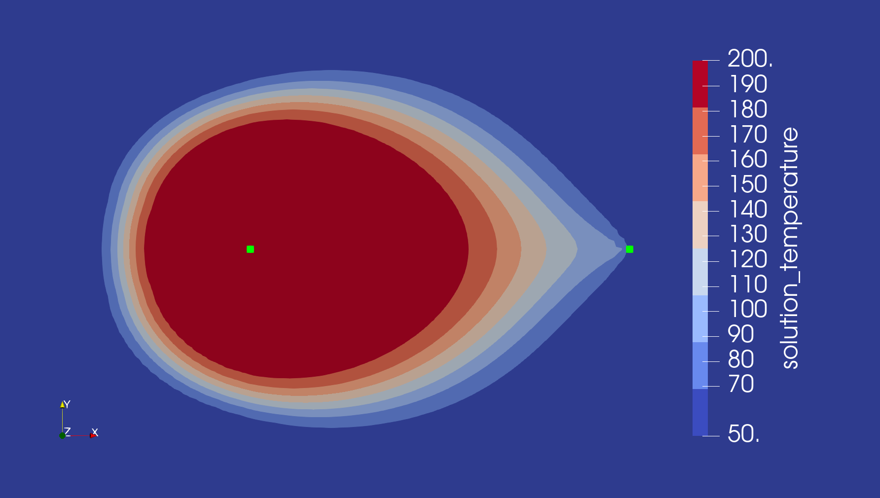
Figure 2: Aquifer temperature after injection of heated aquifer-brine into the system. The green dots show the injection and production borehole positions.
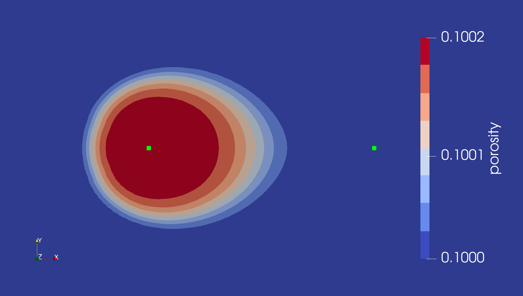
Figure 3: Aquifer porosity after injection of heated aquifer-brine into the system that causes dissolution of the aquifer quartz. The green dots show the injection and production borehole positions.
Comparison with QuartzUnlike
A very similar set of simulations, aquifer_un_quartz_geochemistry.i and exchanger_un_quartz.i may be found in the same directory. Instead of QuartzLike, these use the QuartzUnlike mineral, which precipitates upon heating rather than cooling. It is expected that the hot-fluid injection will have little impact upon the aquifer structure, but that lots of QuartzUnlike will precipitate in the heat exchanger as it heats the produced reservoir fluid. Indeed, the following figure shows this occurs:
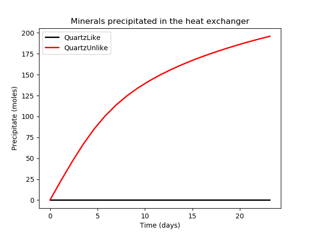
Figure 4: Minerals precipitated in the heat exchanger for the QuartzLike and QuartzUnlike cases. There are no QuartzLike precipitates because it becomes more soluble as it is heated, in contrast to the QuartzUnlike mineral.